A new parton model for the soft interactions at high energies: two channel approximation.

Abstract

The primary goal of this paper is to describe the diffraction production using the model that takes into account the Pomeron interaction, and satisfies both $t$ and $s$ channel unitarity. We hope that these features will allow us to describe the diffraction production in a more convenient way than in CGC motivated models, that do not satisfy these unitarity constraints. Unfortunately, we show that both approaches are only able to describe half of the cross section for the single diffraction production, leaving the second half to be estimates of the large mass production in the Pomeron approach. The impact parameter dependance of the scattering amplitudes show that soft interactions at high energies measured at the LHC, have a much richer structure than presumed. We discuss the $t$-dependence of the elastic cross section in wide range of $|t|=0\div 1\,GeV^{2}$. We show that in the kinematic region of the minimum, we cannot use approximate formulae to calculate the real part of the amplitude. The exact calculation in our model, shows that the real part is rather small, and it is necessary to include the Odderon contribution in order to describe the experimental data.

I Introduction

In our recent paper GLPPM we proposed a new parton model for high energy soft interactions, which is based on Pomeron calculus in 1+1 space-time dimensions, suggested in Ref. KLL , and on simple assumptions of hadron structure, related to the impact parameter dependence of the scattering amplitude. This parton model stems from QCD, assuming that the unknown non-perturbative corrections lead to determining the size of the interacting dipoles. The advantage of this approach is that it satisfies both the $t$-channel and $s$-channel unitarity, and can be used for summing all diagrams of the Pomeron interaction including Pomeron loops. Hence, we can use this approach for all possible reactions: dilute-dilute (hadron-hadron), dilute-dense (hadron-nucleus) and dense-dense (nucleus-nucleus) parton system scattering.

In other words, in this model we assume that the dimensional scale, that determines the interaction at high energy, arises from the non-perturbative QCD approach, which fixes the size of dipoles. Such an approach is quite different from the Colour Glass Condensate (CGC) one, where this scale originates from the interaction of dipoles at short distances, and turns out to be large and increases with energyKOLEB . In spite of the fact, that the model, based on CGC approachGLP1 ; GLP2 ; GLMNI ; GLM2CH ; GLMINCL ; GLMCOR ; GLMSP ; GLMACOR , describes all available data on soft interactions at high energy as well as the deep inelastic processes, it has an intrinsic problem: the CGC approach, in it’s present form, does not provide a scattering amplitude, that satisfies both the $t$ and $s$ channel unitarityKLL .

We have shown that the new parton model is able to describe high energy data on the total and elastic cross sections for proton-proton scattering, but the simple version of Ref.GLPPM leads to vanishing of diffractive production. In this paper we propose a two channel model which generates diffraction production in the region of small masses. As it is well known from the experiences (see for example Refs.GLM2CH ; KMR ) that diffraction production is the process, which is difficult to describe and, specifically, this process provides a check of our approach to long distances physics, which is part of non-perturbative QCD.

We demonstrate that a two channel model is able to describe four experimental observables: $\sigma_{\rm tot}$,$\sigma_{\rm el}$, $B_{\rm el}$ and the single diffraction cross sections. We show that this model leads to a rich structure for the impact parameter dependence of the scattering amplitude. In particular, we study the dependence of the elastic cross section as function of $|t|=0\div 1\,GeV^{2}$. We show that we are able to describe the experimental data on $d\sigma_{el}/dt$ in this $t$-region: the position of the minimum with $|t|_{min}=0.52\,GeV^{2}$ at $W=7\,TeV$ and the value and $t$ behaviour for larger $t$.

II The new parton model

II.1 General approach.

As we have discussed in Ref.GLPPM ; KLL the new parton model is based on three ingredients:

1. The Colour Glass Condensate (GCC) approach (see Ref.KOLEB for a review), which can be re-written in the equivalent form as the interaction of BFKL PomeronsAKLL in a limited range of rapidities ( $Y\leq Y_{\rm max}$):

$$Y\,\leq\,\frac{2}{\Delta_{\mbox{\tiny BFKL}}}\,\ln\left(\frac{1}{\Delta^{2}_{\mbox{\tiny BFKL}}}\right)$$ (1)

$\Delta_{\mbox{\tiny BFKL}}$ denotes the intercept of the BFKL PomeronBFKL . In our model $\Delta_{\mbox{\tiny BFKL}}\,\approx\,0.2-0.25$ leading to $Y_{max}=20-30$, which covers all collider energies.

2. The following Hamiltonian:

$${\cal H}_{\rm NPM}=-\frac{1}{\gamma}\bar{P}P$$ (2)

where NPM stands for “new parton model”. $P$ and $\bar{P}$ are the BFKL Pomeron fields. The fact that it is self dual is evident. This Hamiltonian in the limit of small $\bar{P}$ reproduces the Balitsky-Kovchegov Hamiltonian ${\cal H}_{\rm BK}$ ( see Ref.KLL for details). This condition is the most important one for determining the form of ${\cal H}_{\rm NPM}$. $\gamma$ in Eq. (2) denotes the dipole-dipole scattering amplitude, which in QCD is proportional to $\bar{\alpha}_{S}^{2}$.

3. The new commutation relations:

$$\Big{(}1\,\,-\,\,P\Big{)}\Big{(}1\,\,-\,\,\bar{P}\Big{)}\,\,=\,\,(1-\gamma)\Big{(}1\,\,-\,\,\bar{P}\Big{)}\Big{(}1\,\,-\,\,P\Big{)}$$ (3)

For small $\gamma$ and in the regime where $P$ and $\bar{P}$ are also small, we obtain

$$[P,\bar{P}]=-\gamma+...$$ (4)

consistent with the standard BFKL Pomeron calculus (see Ref.KLL for details) .

In Ref.KLL , it was proved that the scattering matrix for the model is given by

$$S^{\rm NPM}_{m\bar{n}}(Y) = e^{\frac{1}{\gamma}\int_{0}^{Y}d\eta\left[\ln(1-p)\frac{\partial}{\partial\eta}\ln(1-\bar{p})+\bar{p}p\right]}[1-p(Y)]^{m}[1-\bar{p}(0)]^{\bar{n}}|_{p(0)=1-e^{-\gamma\bar{n}};\ \bar{p}(Y)=1-e^{-\gamma m}}$$ (5)

$$= [1-p(Y)]^{m}\,e^{\frac{1}{\gamma}\int_{0}^{Y}d\eta\left[\ln(1-\bar{p})+\bar{p}\right]p}$$

where $p(\eta)$ and $\bar{p}(\eta)$ are solutions of the classical equations of motion and have the form:

$$P(\eta)\,=\,\frac{\alpha+\beta e^{(1-\alpha)\eta}}{1+\beta e^{(1-\alpha)\eta}};\ \ \ \ \bar{P}(\eta)=\frac{\alpha(1+\beta e^{(1-\alpha)\eta})}{\alpha+\beta e^{(1-\alpha)\eta}};$$ (6)

where the parameters $\beta$ and $\alpha$ should be determined from the boundary conditions:

$$P(\eta=0)\,=\,p_{0};\,\,\,\,\,\,\,\,\bar{P}(\eta=Y)\,=\,\frac{\alpha}{P(\eta=Y)}\,=\,\bar{p}_{0}$$ (7)

It is interesting to compare the scattering amplitude given by this expression to that obtained from the BK equation, which describes deep inelastic scattering on nuclei in QCD. For which we have

$$S^{\rm BK}_{m\bar{n}}(Y)=\int dP(\eta)d\bar{P}(\eta)e^{\frac{1}{\gamma}\int_{0}^{Y}d\eta\left[\ln(1-P)\frac{\partial}{\partial\eta}\ln(1-\bar{P})-\ln(1-\bar{P})PP\right]}(1-P(Y))^{m}(1-\bar{P}(0))^{\bar{n}}$$ (8)

In the classical approximation

$$S^{\rm BK}_{m\bar{n}}(Y) = e^{\frac{1}{\gamma}\int_{0}^{Y}d\eta\left[\ln(1-p)\frac{\partial}{\partial\eta}\ln(1-\bar{p})-\ln(1-\bar{p})p\right]}[1-p(Y)]^{m}[1-\bar{p}(0)]^{\bar{n}}|_{p(0)=1-e^{-\gamma\bar{n}};\ \bar{p}(Y)=1-e^{-\gamma m}}$$ (9)

$$= [1-p(Y)]^{m}$$

Note, that the solution for $\bar{P}$, is not relevant for the BK amplitude, which is determined entirely by $P(Y)$. On the other hand, the scattering amplitude in the NPM depends on $\bar{P}$. Nevertheless, the two models should be similar in the regime where the BK evolution is valid. The results of the estimates in Ref.KLL shows that in the region close to saturation, the differences between BK and NPM are quite significant.

II.2 Interrelation with QCD.

As has been mentioned, in the limited range of energies, given by Eq. (1), both QCD and our model describe the interaction of the BFKL PomeronsBFKL . For weak fields $P$ and $\bar{P}$, the model reproduces the BK limit of the CGC approach, assuming that the non-perturbative corrections result in determining the size of the interacting dipoles, and hence, the successful description of the soft data at high energies in CGC approach GLP1 ; GLP2 ; GLMNI ; GLM2CH ; GLMINCL ; GLMCOR ; GLMSP ; GLMACOR supports the idea that this effective size is rather small. The model leads to the descriptions that satisfy both $t$-unitarity and $s$-channel unitarity, while, as it was shown in Ref.KLL , the BFKL Pomeron calculus in the BK limit, as well as the Braun HamiltonianBRAUN for dense-dense system scattering violates $s$-channel unitarity. Unfortunately, we are still far from being able to solve this problem in the effective QCD theory at high energy (i.e. in the CGC /saturation approach).

II.3 Two channel approximation

Our model includes three essential ingredients: (i) the new parton model for the dipole-dipole scattering amplitude that has been discussed above; (ii) the simplified two channel model that enables us to take into account diffractive production in the low mass region, and (iii) the assumptions for impact parameter dependence of the initial conditions.

In the two channel approximation we replace the rich structure of the diffractively produced states, by a single state with the wave function $\psi_{D}$. The observed physical hadronic and diffractive states are written in the form

$$\psi_{h}\,=\,\alpha\,\Psi_{1}+\beta\,\Psi_{2}\,;\,\,\,\,\,\,\,\,\,\,\psi_{D}\,=\,-\beta\,\Psi_{1}+\alpha\,\Psi_{2};~{}~{}~{}~{}~{}~{}~{}~{}~{}\mbox{where}~{}~{}~{}~{}~{}~{}~{}\alpha^{2}+\beta^{2}\,=\,1;$$ (10)

Functions $\psi_{1}$ and $\psi_{2}$ form a complete set of orthogonal functions $\{\psi_{i}\}$ which diagonalize the interaction matrix ${\bf T}$

$$A^{i^{\prime}k^{\prime}}_{i,k}=<\psi_{i}\,\psi_{k}|\mathbf{T}|\psi_{i^{\prime}}\,\psi_{k^{\prime}}>=A_{i,k}\,\delta_{i,i^{\prime}}\,\delta_{k,k^{\prime}}.$$ (11)

The unitarity constraints take the form

$$2\,\mbox{Im}\,A_{i,k}\left(s,b\right)=|A_{i,k}\left(s,b\right)|^{2}+G^{in}_{i,k}(s,b),$$ (12)

where $G^{in}_{i,k}$ denotes the contribution of all non diffractive inelastic processes, i.e. it is the summed probability for these final states to be produced in the scattering of a state $i$ off a state $k$. In Eq. (12) $\sqrt{s}=W$ denotes the energy of the colliding hadrons and $b$ denotes the impact parameter. In our approach we used the solution to Eq. (12) given by Eq. (5) and

$$A_{ik}\,=\,1-S^{\rm NPM}_{ik}(Y)$$ (13)

II.4 The general formulae.

Initial conditions: Following Ref.GLPPM we chose the initial conditions in the form:

$$p_{i}(b^{\prime})=p_{0i}\,S(b^{\prime},m_{i})~{}~{}~{}\mbox{with}~{}~{}S(b,m_{i})=m_{i}bK_{1}(m_{i}b);~{}~{}~{}~{}~{}\bar{p_{i}}(\boldsymbol{b}-\boldsymbol{b})=p_{0i}S(\boldsymbol{b}-\boldsymbol{b}^{\prime},m_{i})~{}~{}~{}~{}~{}~{}~{}z_{m}=e^{\Delta(1-p_{01})Y}$$ (14)

Both $p_{0i}$ and masses $m_{i}$, as well as the Pomeron intercept $\Delta$, are parameters of the model, which are determined by fitting to the relevant data. Note, that $S\left(b,m_{i}\right)\xrightarrow{m_{i}\,b\gg 1}\,\exp\left(-m_{i}\,b\right)$ in accord with the Froissart theoremFROI ,

From Eq. (14) we find that

$$a_{ik}(b,b^{\prime})\,\equiv\,a_{i,k}\left(p_{i},\bar{p}_{k},z_{m}\right) = \,\frac{1}{2}\left(p_{i}+\bar{p}_{k}\right)\,+\,\frac{1}{2\,z_{m}}\left((1-p_{i})(1-\bar{p}_{k})\,-\,D_{i,k}\right);$$ (15)

$$b_{i,k}(b,b^{\prime})\,\equiv\,b_{i,k}\left(p_{i},\bar{p}_{k},z_{m}\right)\,\, = \,\frac{1}{2}\frac{p_{i}-\bar{p}_{k}}{1-p_{i}}-\frac{1}{2z_{m}(1-p_{i})}\left((1-p_{i})(1-\bar{p}_{k})-D_{i,k}\right);$$ (16)

$$~{}~{}D_{i,k} = \sqrt{4p_{i}(1-p_{i})(1-\bar{p}_{k})z_{m}-\left((1-p_{i})(1-\bar{p}_{k})-(p_{i}-\bar{p}_{k})z_{m}\right)^{2}};$$ (17)

These equation are the explicit solutions to Eq. (6) and Eq. (7).

Amplitudes: In the following equations $p_{i}\equiv p_{i}(b^{\prime})$ and $\bar{p}_{k}\equiv\bar{p_{k}}(\boldsymbol{b}-\boldsymbol{b}^{\prime})$.

$$z=e^{\Delta\,(1-p_{01})\,y}$$

$S_{ik}(a_{ik},b_{ik},z)\equiv S(a_{ik}(b,b^{\prime}),b_{ik}(b,b^{\prime}),z_{m})$, $X_{i,k}(a,b,z)\equiv X(a_{ik}(b,b^{\prime}),b_{ik}(b,b^{\prime}),z_{m})$

$$X(a_{ik},b_{ik},z))=\frac{a_{ik}+b_{ik}z}{1+b_{ik}z}$$ (18)

$$SS_{ik}(a_{ik},b_{ik},z)=$$ (19)

$$-(a_{ik}-1)\text{Li}_{2}(-b_{ik}z)+a_{ik}\text{Li}_{2}\left(-\frac{b_{ik}z}{a_{ik}}\right)+(a_{ik}-1)\text{Li}_{2}\left(\frac{a_{ik}+b_{ik}z}{a_{ik}-1}\right)+\frac{1}{2}a_{ik}\log^{2}((1-a_{ik})b_{ik}z)$$

$$-(a_{ik}-1)\log(b_{ik}z+1)\log((1-a_{ik})b_{ik}z)-\left(a_{ik}\log(z)-(a_{ik}-1)\log\left(-\frac{b_{ik}z+1}{a_{ik}-1}\right)\right)\log(a_{ik}+b_{ik}z)$$

$$+a_{ik}\log(z)\log\left(\frac{b_{ik}z}{a_{ik}}+1\right)$$

$$S_{ik}(a_{ik},b_{ik},z)\,\,=\,\,SS_{ik}(a_{ik},b_{ik},z)\,-\,SS_{ik}(a_{ik},b_{ik},z=1)$$ (20)

The amplitude is given by

$$A_{ik}(s,b)\,=$$ (21)

$$\,1-\exp\Bigg{(}\frac{1}{p_{01}}\int\frac{m^{2}_{1}d^{2}b^{\prime}}{4\pi}\Big{(}S_{ik}(a_{ik},b_{ik},z_{m})\,\,+\,\,a_{ik}(b,b^{\prime})\Delta(1-p_{0})Y\Big{)}-\int\frac{m_{1}^{2}d^{2}b^{\prime}}{4\pi}\bar{p}_{k}(\boldsymbol{b}-\boldsymbol{b}^{\prime},m_{k})\,X(a_{ik},b_{ik},z_{m})\Bigg{)}$$

II.5 Physical observables.

The physical observables in this model can be written as follows

$$\mbox{elastic~{}~{} amplitude}: a_{el}(s,b)\,=\,i\left(\alpha^{4}A_{1,1}\,+\,2\alpha^{2}\,\beta^{2}\,A_{1,2}\,+\,\beta^{4}A_{2,2}\right);$$ (22)

$$\mbox{elastic cross section}: \sigma_{tot}\,=\,2\int d^{2}b\,a_{el}\left(s,b\right);~{}~{}~{}\sigma_{el}\,=\,\int d^{2}b\,|a_{el}\left(s,b\right)|^{2};$$

$$\mbox{elastic~{}~{}~{}\, slope}: B_{el}\,=\,\frac{1}{2}\frac{\int b^{2}\,d^{2}b\,\mbox{Im}A_{el}(Y,b)}{\int d^{2}b\,\mbox{Im}A_{el}(Y,b)};$$ (23)

$$\mbox{optical~{}~{}~{}\, theorem}: 2\,\mbox{Im}A_{el}(s,t=0)\,=\,2\int d^{2}b\,\mbox{Im}a_{el}(s,b)\,=\,\sigma_{el}+\sigma_{in}\,=\,\sigma_{tot};$$ (24)

$$\mbox{elastic~{}~{}~{}\,cross section}: \frac{d\,\sigma_{el}}{dt}\,\,=\,\,\pi\,|f(s,t)|^{2};\,\,\,\,\,a_{el}(s,b)\,\,=\,\,\frac{1}{2\,\pi}\int d^{2}q\,e^{-i\boldsymbol{q}\cdot\boldsymbol{b}}\,f\left(s,t\right)\mbox{where}\,\,t\,=\,-q^{2};$$ (25)

$$\mbox{single ~{} diffraction}: \sigma^{GW}_{sd}\,=\,2\,\int\,d^{2}b\,\left(\alpha\beta\{-\alpha^{2}A_{1,1}+(\alpha^{2}-\beta^{2})A_{1,2}+\beta^{2}A_{2,2}\}\,\right)^{2};$$ (26)

$$\mbox{double \,\,diffraction}: \sigma^{GW}_{dd}\,\,=\,\,\,\int d^{2}b\,\,\alpha^{4}\beta^{4}\left\{A_{1,1}\,-\,2\,A_{1,2}\,+\,A_{2,2}\right\}^{2}.$$ (27)

It should be noted, that factor 2 in Eq. (26) takes into account the single diffractive dissociation of the two protons.

III Comparison with experimental data for proton-proton scattering

III.1 The results of the fit in two channel model

As we have seen in the previous section, we introduce three dimensionless parameters: $\Delta$ - the intercept of the BFKL Pomeron, and $p_{01}$ ($p_{02}$) - the amplitudes of the dipole-dipole scattering at low energies, and $\beta$ which is related to the contribution of the diffractive production. For $b$-dependence we suggested a specific form (see Eq. (14)) which is characterized by the dimensional parameters: $m_{i}$. These parameters are determined by fitting to the experimental data. We choose to describe five observables: total and elastic cross sections, the elastic slope and single and double diffractions at low masses (see Eq. (22)-Eq. (27)).

The situation with the experimental data on the single and double diffraction production in proton-proton scattering at high energies, is far from clear. It was well summarized in Ref.KMR , to which we refer the reader. We assume that the two channel model is able to describe proton-proton diffraction production in the entire kinematic region of produced mass. As is shown in Ref.GUGU for $\Delta\,>\,0$ the integral over the produced mass in diffraction is convergent, and the Good-Walker mechanismGW is able to describe the diffraction production both of small and large masses. However, the simple two channel model is a simplification, but we hope to learn something by attempting to fit all available data using this simple model.

From Fig. 1 one can see that we obtain quite a good description of the data for $\sigma_{tot},\sigma_{el}$ and for the slope $B_{el}$ for $W\geq 0.5\,TeV$. Comparing with the one channel model of Ref.GLPPM we start fitting from lower value of $W=0.5\,TeV$ instead of $W=1\,TeV$. We present The fitting parameters in Table I. One can see that both sets have the same qualitative features: the large value of the amplitude $A_{1,1}$ and small values of other amplitudes. Note, the values of parameters which describe this large amplitude turns out to be quite different in one and two channels fits . Especially, this difference is seen in the value of $\Delta$ and masses ($m_{1}$ and $m_{2}$). The quality of the description of this model and the one channel model of Ref.GLPPM for $W=0.5\div 13\,TeV$ are more or less the same . However for $W>1\,TeV$ the one channel model gives a better description.

However, from Fig. 5-a and Fig. 6-a it is clear that we failed to describe the data on the single and double diffraction production: roughly speaking we are able to describe only half of the values for single diffraction cross section. Therefore, the simple two channel model is not enough to describe the experimental data on the single diffraction production, in spite of the three new parameters that we have introduced. Actually, we had the same situation in our CGC motivated model of Ref.GLM2CH . Hence, we can conclude that the fact that our model satisfies the unitarity constraints both in $t$ and $s$ channel unitarity is not sufficient, and we need to search for a more complicated model for the hadron structure.

The values of parameters which led to the best agreement with the experimental data of are shown in Table I. The two sets of parameters are quite different, but qualitatively they describe the data with large $A_{1,1}$ and small $A_{1,2}$ and $A_{2,2}$.

Comparing these parameters with the resulting curves in Fig. 1 we see that shadowing corrections play an essential role. First, we note that the value of $\Delta_{\rm dressed}\,\,=\,\,\Delta\left(1-p_{01}\right)$ is rather large (about 0.5) in all variants. Recall, that means that $\Delta\approx 1$. Factor $(1-p_{01})$ in $\Delta_{\rm dressed}$, stems from the enhanced diagrams that contribute to the Green function of the Pomeron. The resulting $\sigma_{\rm tot}\,\propto\,s^{\Delta_{\rm eff}}$ with $\Delta_{\rm eff}\approx 0.07$. The reduction from $\Delta_{\rm dressed}$ to $\Delta_{\rm eff}$ occurs due to strong shadowing corrections.

From Fig. 6-a one can see that we failed to describe the double diffraction production. This reflects the situation which we had in our previous attempts to describe this processGLM2CH . The same problem occurs with other groups (see, for example, Ref.KMR and reference therein). The small size of the double diffraction cross section in our model occurs since the main contribution stems from the amplitude $A_{1,1}$ which is close to 1. Bearing this in mind we see that $\sigma_{dd}\,\,\approx\,\,\frac{\beta^{4}}{\alpha^{4}}\sigma_{el}$ and since $\frac{\beta^{4}}{\alpha^{4}}$ = (1/16 set I) (0.03 set II) the cross section turns out to be small.

Variant of the fit	$\Delta_{\rm dressed}$	$p_{01}$	$p_{02}$	$m_{1}$ (GeV)	$m_{2}$(GeV)	$\beta^{2}$
I	0.488 $\pm$ 0.002	0.748 $\pm$ 0.002	0.005 $\pm$ 0.001	1.03 $\pm$ 012	0.49 $\pm$ 0.08	0.134 $\pm$ 0.003
II	0.499$\pm$ 0.01	0.972 $\pm$ 0.02	0.166 $\pm$ 0.001	1.05 $\pm$ 0.01	1.44 $\pm$ 0.020	0.2 $\pm$ 0.01
One channel	0.33 $\pm$ 0.03	0.489 $\pm$ 0.030		0.867 $\pm$ 0.005		0

Table 1: Fitted parameters.$\Delta_{\rm dressed}=\Delta\left(1-p_{01}\right)$.

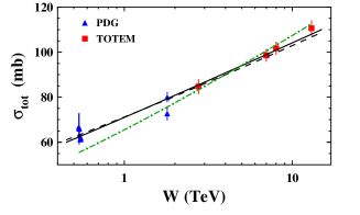
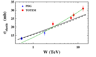
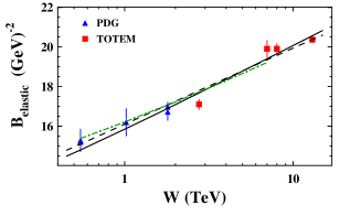
Fig. 1-a	Fig. 1-b	Fig. 1-c

Figure 1: The energy behaviour of $\sigma_{tot},\sigma_{el}$ and the slope $B_{el}$ for proton-proton scattering in our model. The solid line describes the variant I in Table I while the dashed line corresponds to variant II. Data are taken from Refs.PDG ; TOTEMRHO .

III.2 Diffraction production of large masses

The natural source of diffraction production, which we neglected in our two channel model, is the production of large masses which can be reduced to the tripple Pomeron diagrams. Fig. 2-a and Fig. 2-b illustrate how the production of large mass is related to the exchange of the Pomerons. As we have discussed, our model is based on the theoretical approach that describes the Pomerons and their interaction and, therefore, we can estimate the contribution of the large mass to the diffraction production without introducing any new parameters. In particular, the first diagram of Fig. 2-b takes the form:

$$\sigma^{\rm LM}_{\rm sd}\,\,=\,\,2\,\int^{Y}_{0}\,dy^{\prime}\,\int d^{2}b^{\prime}\,p_{i}\,G_{I\!\!P}\left(Y-y^{\prime},\boldsymbol{b}-\boldsymbol{b}^{\prime}\right)\Gamma_{3{I\!\!P}}\,G^{2}_{I\!\!P}\left(y^{\prime},\boldsymbol{b}^{\prime}\right)\,p^{2}_{k}$$ (28)

where the triple Pomeron vertex $\Gamma_{3{I\!\!P}}$ is known in our model, as well as the vertices of Pomeron interaction with the states 1 and 2 ($p_{1},p_{2}$). $G_{I\!\!P}\left(y,b\right)$ is the Green’s function of the Pomeron. The factor 2 in front follows from the unitarity constraint for the Pomeron : $\sigma_{I\!\!P}\,=\,2\,G_{I\!\!P}$.

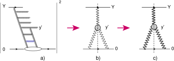
Figure 2: The single diffraction production of large masses. Fig. 2-a and Fig. 2-b present the first diagrams for the diffraction production. The blog represents the triple Pomeron vertex. Fig. 2-c corresponds to the contributions of the ‘dressed ’ Pomerons in our model. The wavy lines denote the Pomeron while the double wavy lines describe the resulting Green’s function of the Pomeron in our model

We have the same expression as in Eq. (28) for the diagram of Fig. 2-c but we need to replace the bare Pomeron Green’s function by the resulting (‘dressed’) Pomeron Green’s function ($G_{I\!\!P}\left(y,b\right)\,\,\to\,\,G^{\rm dresssed}_{I\!\!P}\left(y,b\right)$). In our model it turns out that easier to find not the resulting Green’s function but the product $p_{i}\,G^{\rm dresssed}_{I\!\!P}\left(y,b\right)$, which we will denote $\tilde{A}_{i,{I\!\!P}}\left(y,b\right)$. We can find this amplitude from the general formulae of section II applying new initial conditions instead of Eq. (14): viz.

$$p_{i}\left(b\right)\,=\,p_{0i}S\left(b,m_{i}\right)\,\,\,\mbox{for}\,\,\,\,i=1,2;~{}~{}~{}~{}~{}~{}~{}p_{I\!\!P}\left(b\right)\,=\,p_{0,{I\!\!P}}\,S\left(b,m_{I\!\!P}\right)$$ (29)

From our model it follows that $p_{0,{I\!\!P}}\,=\,p_{01}$, but the value of the mass $m_{I\!\!P}$ should include the impact parameter dependence of the triple Pomeron vertex. It is known that the radius of the triple Pomeron vertex is much smaller that the size of the proton. We choose the typical mass $m_{I\!\!P}=3\,GeV$, which means that this radius is in about three times smaller than the radius of the Pomeron-proton vertex. We checked that the numerical estimates are not sensitive to the value of this mass.

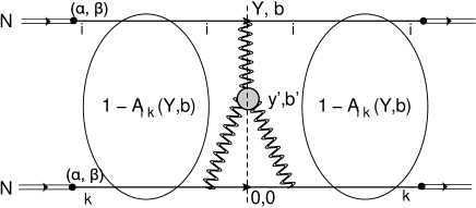
Figure 3: The single diffraction production of large masses including the survival probability. The wavy lines denote the Pomeron, while the double wavy lines describe the resulting Green’s function of the Pomeron in our model . The black circles denote the transition $<\psi_{h}|\psi_{i}>\,=\,\alpha(i=1)$ or $\beta(i=2)$.

However, we need to multiply Eq. (28) by the survival probability (see Refs. KMRREV ; GLMREV for a review). Indeed, together with the processes shown in Fig. 2 a number of parton showers can be produced and gluons (quarks) from these showers will produce additional hadrons which, in particular, can fill the rapidity gap ($y^{\prime}$ in Fig. 2). The survival probabilty factor $\langle S^{2}\rangle$ gives the fraction of the processes in which the production of the parton showers are suppressed. Finally, the contribution of the single diffraction is given by the following expression (see Fig. 3):

$$\sigma^{\rm LM}_{\rm sd}\,\,=\,\,2\,\int^{Y}_{0}\,dy^{\prime}\,\int d^{2}b^{\prime}\,\,\tilde{A}_{i,{I\!\!P}}\left(Y-y^{\prime},\boldsymbol{b}-\boldsymbol{b}^{\prime}\right)\tilde{A}^{2}_{k,\ {I\!\!P}}\left(y^{\prime},\boldsymbol{b}^{\prime}\right)\,\Big{(}1\,\,-\,\,A_{i,k}\left(Y,b\right)\Big{)}^{2}$$ (30)

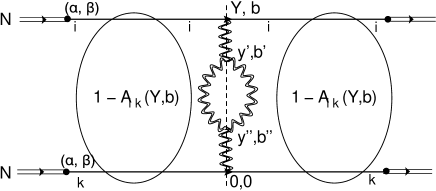
Figure 4: The double diffraction production of large masses including the survival probability. The double wavy lines describe the resulting Green’s function of the Pomeron in our model. The black circles denote the transition $<\psi_{h}|\psi_{i}>\,=\,\alpha(i=1)$ or $\beta(i=2)$.

The main contribution to $\sigma^{\rm LM}_{\rm sd}$ for set I, stems from $A_{1,1}$, in spite of small values of $\langle S^{2}\rangle$, since all other amplitude are small. For set II $A_{1,2}$ leads to the largest cross section due to large $\langle S^{2}\rangle\approx 0.8$.

For double diffraction in the region of large masses we can write the following formula which follows directly from Fig. 4:

$$\sigma_{\rm dd}\,\,=$$ (31)

$$4\,\int^{Y}_{0}\,dy^{\prime}\,\int^{y^{\prime}}_{0}d\,y^{\prime\prime}\,\int d^{2}b^{\prime}\,\int d^{2}b^{\prime\prime}\,\,\tilde{A}_{i,{I\!\!P}}\left(Y-y^{\prime},\boldsymbol{b}-\boldsymbol{b}^{\prime}\right)\tilde{A}^{2}_{{I\!\!P},{I\!\!P}}\left(y^{\prime}-y^{\prime\prime},\boldsymbol{b}^{\prime}-\boldsymbol{b}^{\prime\prime}\right)\,\tilde{A}_{k,{I\!\!P}}\left(y^{\prime\prime},\boldsymbol{b}-\boldsymbol{b}^{\prime}\right)\Big{(}1\,\,-\,\,A_{i,k}\left(Y,b\right)\Big{)}^{2}$$

III.3 Diffraction production: comparison with the experimental data

Fig. 5-a shows a comparison of our results compared to the single diffraction production data, taken from Ref.KAS and which are shown in Fig. 5-b. One can see that the description is not very good at $W\,\approx\,0.5\,TeV$. The reason for this is that, the integration over $y^{\prime}$ in Eq. (30) leads to the amplitude $A_{i,{I\!\!P}}$ and $A_{k,{I\!\!P}}$ enter at energies smaller than $W=0.5\,TeV$. We cannot describe these energies in our model. For larger energies the phase space that corresponds to the unknown region of energies gives much smaller contributions.

The TOTEM value of the single diffraction cross section is $9.1\pm 2.9$ (see Ref.KAS ) , while our estimates lead to $\sigma^{\rm smd}_{\rm sd}=12-13mb$. As can be seen from Fig. 5-a and Fig. 5-b, our model leads to values of the single diffraction cross section, which are close to our predictions from the CGC motivated model of Ref.GLM2CH (the curve GLM in Fig. 5-b). We refer the reader to Ref.KMR in which the situation with tensions between different experimental groups on the single diffraction cross section, has been discussed.

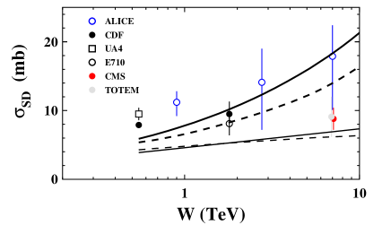
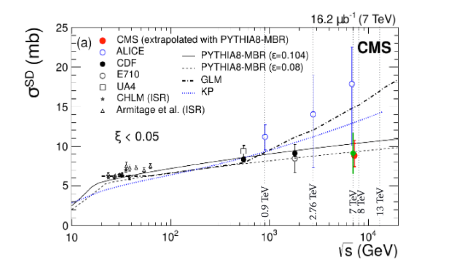
Fig. 5-a	Fig. 5-b

Figure 5: The single diffraction cross section as function of energy $W=\sqrt{s}$: our description of the data with $W\geq\,0.5\,TeV$ (Fig. 5-a) and the experimental data from Ref.KAS (Fig. 5-b). The solid and dashed lines in Fig. 5-a correspond to set I and set II (see Table I),respectively. The upper lines show the sum of small and large masses diffraction, while the lower ones present the small mass diffraction that were fitted in our model. The data of all experimental groups were extrapolated to the region $M^{2}\leq 0.05\,s$ using the Pythia Monte-Carlo programs as is shown in Fig. 5-b. $M$ is the mass of hadron produced in single diffraction. The data in Fig. 5-a are taken from Ref.KAS and we refer to this paper (especially to Ref.[9] in it). The curves in Fig. 5-b marked as GLM are taken from Ref.GLM2CH and that as KP is from Ref.KAPO .

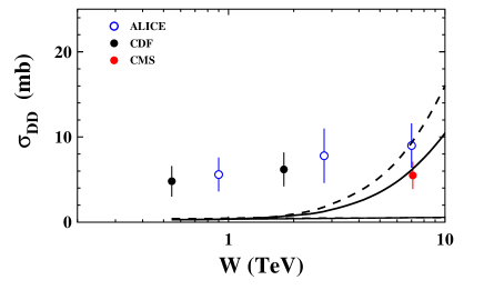
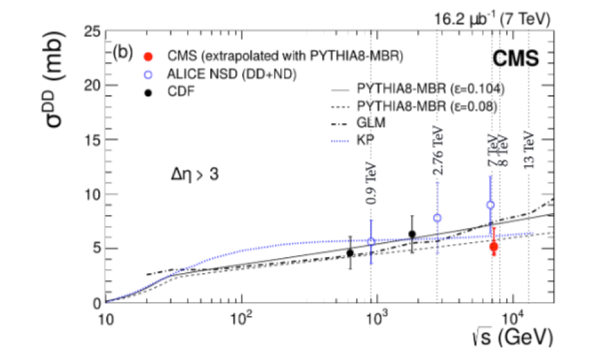
Fig. 6-a	Fig. 6-b

Figure 6: The double diffraction cross section as function of energy $W=\sqrt{s}$.The solid and dashed lines in Fig. 6-a correspond to set I and set II (see Table I),respectively. The upper lines show the sum of small and large masses diffraction, while the lower ones present the small mass diffraction that were fitted in our model. The experimental points, were taken from Ref.KAS .

The description of the double diffraction is very poor. The large mass diffraction leads to a large double diffraction cross section at high energies, and we cannot reproduce the values of $\sigma_{dd}$ at lower energies.

Concluding this section we can claim that the large mass diffraction leads to a considerable contribution, which in this model increases rapidly with energy. This is a direct consequence of the large value of $\Delta_{\rm dressed}$ in our model (see Table I). For $W\,>\,0.5\,TeV$, this increase is damped by large shadowing corrections, but in the formulae for diffraction production of large masses, includes energies which are less than $W\,=\,0,5$, where the strength of shadowing corrections is not sufficient to lead to a reasonable effective $\Delta$.

IV Dependence on impact parameters

In Fig. 7 we plot the scattering amplitudes as a function of the impact parameter b. One can see that the two channel model generates a very interesting and unexpected structure. One amplitude $A_{11}(b)$ has reached the unitary limit $A_{11}\left(b=0\right)=1$ at $W=0.5\,TeV$ and shows the increasing of the radius of the interaction, with energy. The two other amplitudes are far from the unitarity limit even at ultra high energy $W=100\,TeV$. They increase as $W^{\Delta_{\rm eff}}$ with $\Delta_{\rm eff}\sim 0.1$. The behaviour as a function of $b$ is also unexpected. Both $A_{11}$ and $A_{22}$ decrease monotonically at large $b$, while $A_{12}$ has a maximum which moves to larger values of $b$. The value of the amplitude for this maximum increases as $W^{\Delta_{\rm eff}}$. On the other hand, $A_{12}\left(b=0\right)$ is almost independent of $W$.

Such dependence of the amplitudes generate the elastic amplitude which is smaller than the unitarity limit even at very high energies (see Fig. 7-a). This conclusion is in accord with the recent paper of Ref.GSS in which it is demonstrated that in the Miettinen-Pumplin MIPU approach the elastic amplitude $A_{el}\left(b=0\right)\approx 0.92\,<\,1$ at $W=57\,TeV$. Note, that this approach is ideologically close to ours and second, that in Ref.GSS the entire set of soft interaction data has been described successfully.

In Fig. 5-a we present the comparison between the elastic amplitude in our 2 channel model and in one channel model of Ref. GLPPM . One can see that these two amplitudes have a different behaviour both as a function of energy and impact parameter. We believe that this figure demonstrates that the modeling of the non-perturbative structure of the hadron is very important in understanding high energy scattering. Fig. 8-b shows the behaviour of $d\sigma_{\rm sd}/db^{2}$ (see Eq. (26))

$$\frac{d\sigma_{\rm sd}}{db^{2}}\,\,\,=\,\,\,\left(\alpha\beta\{-\alpha^{2}A_{1,1}+(\alpha^{2}-\beta^{2})A_{1,2}+\beta^{2}A_{2,2}\}\,\right)^{2}$$ (32)

One can see that this observable decreases very slowly with energy, and does not show a maximum at large $b$. Such behaviour is quite different from what we obtain in CGC motivated model (see Ref.GLM2CH Fig.7) and from the estimates of Ref.GSS .

We believe that the impact parameter and energy behaviours shown in Fig. 7 and in Fig. 5, illustrate the fact that the soft interaction at high energies could have a much richer structure than we previously assumed.

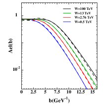
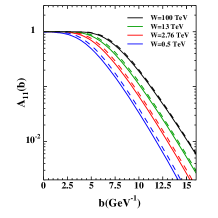
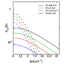
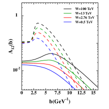
Fig. 7-a	Fig. 7-b	Fig. 7-c	Fig. 7-d

Figure 7: The scattering amplitudes versus impact parameter $b$ for different energies:Fig. 7-a $A_{el}$; Fig. 7-b $A_{11}$, Fig. 7-c $A_{22}$,Fig. 7-d $A_{12}$.

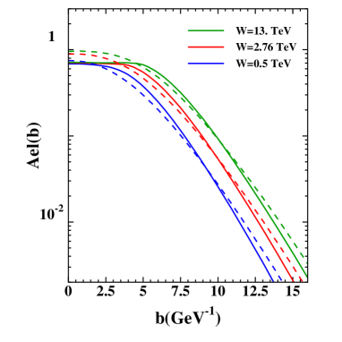
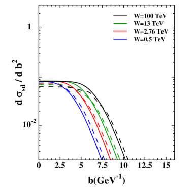
Fig. 8-a		Fig. 8-b

Figure 8: The scattering amplitudes versus impact parameter $b$ for different energies: Fig. 8-a: the elastic amplitudes for the one channel model of Ref.GLPPM (dashed line) and for two channel model of this paper (solid line). For estimates in our model we used set I of parameters in Table I; Fig. 8-b : $\frac{d\sigma_{\rm sd}}{db^{2}}$ of Eq. (32) for the variant two (solid line) and variant one (dashed line) set of parameters.

V Dependence of the elastic cross sections on $t$

We attempt to describe the elastic cross section for $|t|=0\div 1\,GeV^{2}$ to check the rich structure present in the impact parameter dependence, this stems from our model, which predicts the existence of a minimum in the elastic cross sections, however its position occurs at $|t|\,\approx\,0.3\,GeV^{2}$, which is much smaller than was observed experimentally by TOTEM collaborationTOTEMLT .

Assuming that this discrepancy is due to the simplified form of $b$ dependence of our amplitude which is given by Eq. (14), we changed the initial conditions of Eq. (14) to the following equations

$$p_{i}(b^{\prime})=p_{0i}\,S(b^{\prime},m_{i},\mu_{i},\kappa_{i})~{}~{}~{}\mbox{with}~{}~{}S(b,m_{i},\mu_{i},\kappa_{i})=\left(1-\kappa_{i}\right)\left(m_{i}\,b\right)^{\nu_{1}}K_{\nu_{1}}(m_{i}\,b)\,\,+\,\,\kappa_{i}\frac{\left(m_{i}\,b\right)^{\nu_{2}}K_{\nu_{2}}(\mu_{i}\,b)}{2^{\nu_{2}\,-\,1}\,\Gamma\left(\nu_{2}\right)}$$ (33)

As we have seen in Fig. 1 our two channel model does not give a good description of the elastic cross section. Bearing this in mind we made a fit using the one channel model in which $p_{01}\neq 0$ but $p_{o2}=0$. In the Table II we present the parameters that we found for the fit. Fig. 9 shows the comparison with TOTEM data of Ref.TOTEMLT . One can see that we obtain good agreement with the experimental data for $|t|\,<\,|t|_{min}$ and for $|t|\,>\,|t|_{min}$. However, for $|t|\approx\,|t|_{min}$ the real part of the scattering amplitude turns out to be small, and we obtain a value of the $d\sigma_{el}/d\,t$ approximately an order of magnitude smaller than the experimental one. It should be stressed that we do not use any of the simplified approaches to estimate the real part of the amplitude, but using our general expression of Eq. (21) for $A_{ik}\left(s,t\right)$, we consider the sum $A_{ik}\left(s,+i\epsilon t\right)+A_{ik}\left(u-i\epsilon,t\right)$, which corresponds to positive signature, and calculated the real part of this sum.

In Fig. 9 we estimate the contribution of the $\omega$ -reggeon , using the description taken from the paper of Ref.DOLA (note the difference between green dashed line and the blue solid curve). This contribution is small, and can be neglected.

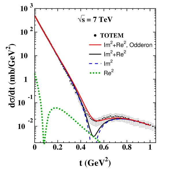
Figure 9: $d\sigma_{el}/dt$ versus $t$. The black green line describes the result of our fit. The dashed line corresponds to the contribution of the imaginary part of the scattering amplitude to the elastic cross section. The dotted line relates to the real part of our amplitude.The red solid line takes into account the contribution of the odderon to the real part of the $pp$ amplitude, as is shown in Eq. (36). The data , shown in grey, include systematic errors. They are taken from Ref.TOTEMLT .

To evaluate the real part of the amplitude we use the relation: However,

$${\rm Re}A_{11}(s,t)\,\,=\,\,\frac{1}{2}\,\pi\,\frac{\partial}{\partial\,\ln\left(s/s_{0}\right)}\,{\rm Im}A_{11}\left(s,t\right)|_{{Eq.~{}(\ref{AIK})}}$$ (34)

Eq. (34) correctly describes the real part of the amplitude only for small $\rho={\rm Re}A/{\rm Im}A$. In Fig. 10 we plot the $d\sigma/dt$ with such estimates for the real part. The real part from Eq. (34) turns out to be almost twice larger than the experimental data in the vicinity of $t_{min}$. Therefore, at the minimum, where ${\rm Im}\,A\,\ll\,{\rm Re}A$, Eq. (34) cannot be used for the real part. However, replacing Eq. (34) by

$${\rm Re}A_{11}(s,t)\,\,=\,\,\tan\left(\rho\right)\,{\rm Im}A_{11}\left(s,t\right)|_{{Eq.~{}(\ref{AIK})}}$$ (35)

we obtain the same result, that the real part of the amplitude turns out to be too large. Actually,Eq. (35) assumes that the scattering amplitude depends on energy as a power $A\left(s,t\right)\,\propto\,s^{2\,\rho/\pi}$. Our amplitude is a rather complex function of energy, and depends on $\ln(s)$.

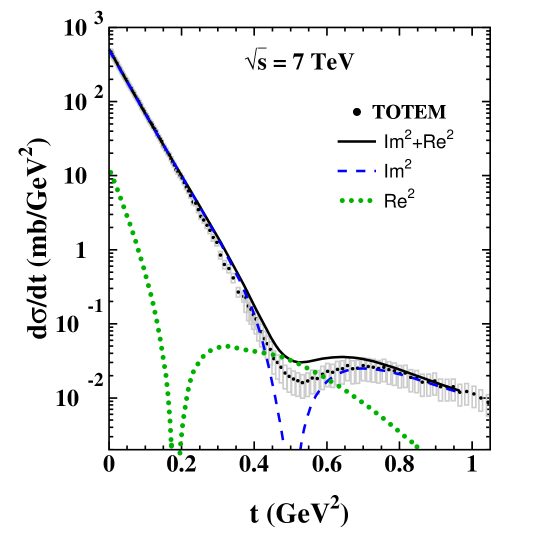
Figure 10: $d\sigma_{el}/dt$ versus $t$. The solid line describes the result of our fit. The dotted line corresponds to the contribution of the real part of the scattering amplitude to the elastic cross section, which is calculated using Eq. (34), with added contribution of the exchange of the $\omega$ - reggeon, which is taken from Ref.DOLA . We do not show the contribution of the real part without the $\omega$-reggeon since it coincides with the dotted line. The dashed line is the contribution of the imaginary part of the amplitude. The data are taken from Ref.TOTEMLT )

Variant of the fit	$\Delta_{\rm dressed}$	$p_{01}$	$m_{1}$ (GeV)	$\mu_{1}$(GeV)	$\nu_{1}$	$\nu_{2}$	$\kappa_{1}$
one channel model	0.48 $\pm$ 0.01	0.8 $\pm$ 0.05	0.860	7.6344	0.9	0.1	0.48

Table 2: Fitted parameters for $d\sigma_{el}/dt$ dependence.$\Delta_{\rm dressed}=\Delta\left(1-p_{01}\right)$.

Concluding, we see that to describe the TOTEM experimental data in the framework of our model, the contribution to the real part of the amplitude from the exchange of the odderonODD is needed. Hence, our estimates confirm the conclusions of Ref.ODDSC . In Fig. 9 we plot the description of the elastic cross section in which we have added the odderon contribution to the amplitude of Eq. (21) (red solid curve in Fig. 9):

$$f\left(s,t\right)\,\,=\,\,f\left(s,t;{Eq.~{}(\ref{AIK})}\right)\,\,\pm\,\,\sigma_{\rm odd}e^{B_{\rm odd}\,t}$$ (36)

where we consider a QCD odderonODD : the state with odd signature and with the intercept $\alpha_{\rm odd}(t=0)=1$, which contributes only to the real part of the scattering amplitude. The value of $\sigma_{\rm odd}\,=\,20.6\,\bar{\alpha}_{S}^{3}\,mb\,\approx\,0.5\,mb$ for $\bar{\alpha}_{S}=0.3$ in Eq. (36) we take from the QCD estimates in Ref.RYODD . The value of $B_{\rm odd}=5.6\,GeV^{-2}$ which is smaller than elastic slope for the BFKL Pomeron in accord with QCD estimatesRYODD . The sign minus in Eq. (36) corresponds to proton-proton scattering, while the sign plus refers to antiproton-proton collisions. Our odderon parameters are in accord with the estimates in Ref.KMR . The amplitude $f(s,t)$ is related to $a_{el}\left(s,b\right)$ by Eq. (25) (see also Eq. (22)).

In Fig. 11 we show the prediction for proton-antiproton scattering. One can conclude that in our model the measurements of the elastic cross sections for $p\,p$ and $\bar{p}p$ scattering can provide the estimates for the odderon contribution. It should be stressed that the contribution of the $\omega$-reggeon leads to negligible contribution at $W=7\,TeV$ (see Fig. 10).

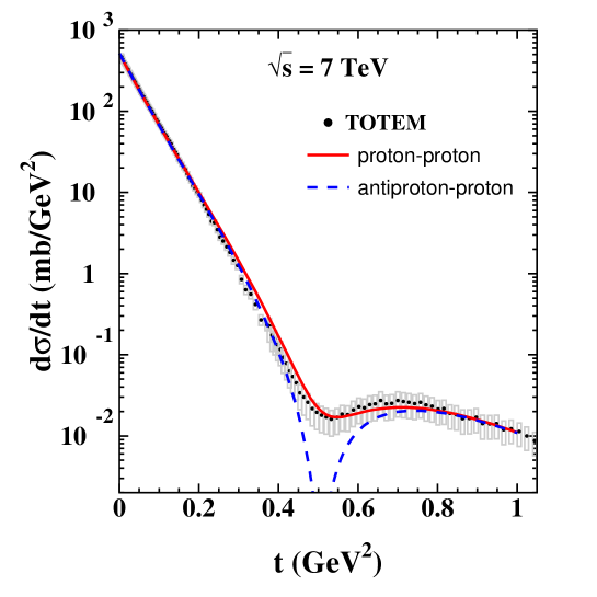
Figure 11: $d\sigma_{el}/dt$ versus $t$. The solid line describes the elastic cross sections for $pp$-scattering with the odderon contribution (see Eq. (36)), while the dashed line shows the elastic cross section for $\bar{p}p$-scattering using Eq. (36). The data are taken from Ref.TOTEMLT )

VI Conclusions

The primary goal of this paper was to investigate whether the new parton model, which has been developed in Ref.GLPPM , is able to describe the diffraction production. The model is based on Pomeron calculus in 1+1 space-time, suggested in Ref. AKLL , and on the simple assumptions on the hadron structure, related to the impact parameter dependence of the scattering amplitude. This parton model stems from QCD, assuming that the unknown non-perturbative corrections lead to fixing the size of the interacting dipoles. The advantage of this approach is that it satisfies both t-channel and s-channel unitarity, and it can be used for summing all diagrams of the Pomeron interaction including the Pomeron loops. Our hope was that this model will be superior to the model which we developed based on CGC approachGLP1 ; GLP2 , and which does not satisfy both $t$ and $s$ channel unitarity.

Unfortunately, we did not find any advantages of our new model, and we have to describe half of the single diffraction cross section by the diffraction production of large masses, in striking similarity with the CGC based models. Certainly, it is not a very encouraging result, especially since the CGC models describe the large mass diffraction production better than this model. Mostly this is due to the fact that $\Delta_{\rm dressed}$ in this model, turns out to be larger than in CGC one.

The impact parameter dependance of the scattering amplitudes (see Fig. 7) shows that the soft interaction at high energies measured at the LHC have a much richer structure that we presumed in the past. We believe that we have demonstrated that the character of high energy scattering is closely related to the structure of hadron, which presently is described by a simple two channel model.

Our attempt to describe the $t$-dependence of the elastic cross section shows that we can reproduce the main features of the $t$-dependence that are measured experimentally: the slope of the elastic cross section at small $t$, the existence of the minima in $t$-dependence which is located at $|t|_{min}=0.52\,GeV^{2}$ at W= 7 TeV; and the behaviour of the cross section at $|t|\,>\,|t|_{min}$. It should be stressed that our model allows us to find the real part of the scattering amplitude using our general expression of Eq. (21) for $A_{ik}\left(s,t\right)$. We consider the sum $A_{ik}\left(s,+i\epsilon t\right)+A_{ik}\left(u-i\epsilon,t\right)$, which corresponds to positive signature, and calculated the real part of this sum. It should be stressed that we do not use any of the simplified approaches to estimate the real part of the amplitude which we show (in our model ) which do not reproduce correctly the real part of the amplitude at large $t$. In our model the real part turns out to be much smaller than the experimental one. Consequently, to achieve a description of the data, it is necessary to add an odderon contribution. Hence, our model corroborates the conclusion of Ref.ODDSC .

A topic for future study, is whether the characteristic behaviour of the $A_{i,k}(b)$ amplitudes as a function of $b$ stems from the theory of interacting Pomerons, which satisfies both $s$ and $t$ channel unitarity, or is an artifact of the simple two channel approach with the phenomenological input, on the impact parameter dependence.

We are aware that our model is very naive in describing the hadron structure, but hope that further progress in accumulating data on diffraction production, as well as the unsolved problem of treating the processes of the multiparticle generation in the framework of our approach, will generate a self consistent picture for high energy scattering at long distances.

Acknowledgements.
We thank our colleagues at Tel Aviv University and UTFSM for encouraging discussions. Our special thanks go to Tamas Csörgő and Jan Kasper for discussion of the odderon contribution and elastic scattering during the Low x’2019 WS. This research was supported by CONICYT PIA/BASAL FB0821(Chile) and Fondecyt (Chile) grants 1170319 and 1180118 .

References

- (1) E. Gotsman, E. Levin and I. Potashnikova, “A new parton model for the soft interactions at high energies,” Eur. Phys. J. C 79 (2019) no.3, 192, [arXiv:1812.09040 [hep-ph]].
- (2) A. Kovner, E. Levin and M. Lublinsky, “QCD unitarity constraints on Reggeon Field Theory,” JHEP 1608 (2016) 031, [arXiv:1605.03251 [hep-ph]].
- (3) Y. V. Kovchegov and E. Levin Quantum chromodynamics at high energy Vol. 33 (Cambridge University Press, 2012).
- (4) E. Gotsman, E. Levin and I. Potashnikova, “CGC/saturation approach: soft interaction at the LHC energies,” Phys. Lett. B 781 (2018) 155, [arXiv:1712.06992 [hep-ph]].
- (5) E. Gotsman, E. Levin and I. Potashnikova, “A CGC/saturation approach for angular correlations in proton - proton scattering,” Eur. Phys. J. C 77 (2017) no.9, 632, [arXiv:1706.07617 [hep-ph]].
- (6) E. Gotsman, E. Levin and U. Maor, “A model for strong interactions at high energy based on the CGC/saturation approach,” Eur. Phys. J. C 75 (2015) 1, 18 [arXiv:1408.3811 [hep-ph]].
- (7) E. Gotsman, E. Levin and U. Maor, “CGC/saturation approach for soft interactions at high energy: a two channel model,” Eur. Phys. J. C 75 (2015) 5, 179 [arXiv:1502.05202 [hep-ph]].
- (8) E. Gotsman, E. Levin and U. Maor, “CGC/saturation approach for soft interactions at high energy: inclusive production,” Phys. Lett. B 746 (2015) 154 [arXiv:1503.04294 [hep-ph]].
- (9) E. Gotsman, E. Levin and U. Maor, “CGC/saturation approach for soft interactions at high energy: long range correlations," Eur. Phys. J. C 75 (2015) 11, 518 [arXiv:1508.04236 [hep-ph]].
- (10) E. Gotsman, E. Levin and U. Maor, “CGC/saturation approach for soft interactions at high energy: survival probability of central exclusive production,” Eur. Phys. J. C 76 (2016) no.4, 177, [arXiv:1510.07249 [hep-ph]].
- (11) E. Gotsman, E. Levin, U. Maor and S. Tapia, “CGC/saturation approach for high energy soft interactions: in proton-proton collisions,” Phys. Rev. D 93 (2016) no.7, 074029, [arXiv:1603.02143 [hep-ph]].
- (12) V. A. Khoze, A. D. Martin and M. G. Ryskin, “Elastic and diffractive scattering at the LHC,” Phys. Lett. B 784, 192 (2018) doi:10.1016/j.physletb.2018.07.054 [arXiv:1806.05970 [hep-ph]].
- (13) T. Altinoluk, A. Kovner, E. Levin and M. Lublinsky, “Reggeon Field Theory for Large Pomeron Loops,” JHEP 1404 (2014) 075 [arXiv:1401.7431 [hep-ph]].
- (14) V. S. Fadin, E. A. Kuraev and L. N. Lipatov,“On the pomeranchuk singularity in asymptotically free theories", Phys. Lett. B60, 50 (1975); E. A. Kuraev, L. N. Lipatov and V. S. Fadin,“The Pomeranchuk Singularity in Nonabelian Gauge Theories" Sov. Phys. JETP 45, 199 (1977), [Zh. Eksp. Teor. Fiz.72,377(1977)]; I. I. Balitsky and L. N. Lipatov,“The Pomeranchuk Singularity in Quantum Chromodynamics,” Sov. J. Nucl. Phys. 28, 822 (1978), [Yad. Fiz.28,1597(1978)]
- (15) M. A. Braun, “Nucleus-nucleus scattering in perturbative QCD with Phys. Lett. B 483, 115 (2000); e-Print Archive:[hep-ph/0003004]; “Nucleus nucleus interaction in the perturbative QCD,” Eur. Phys. J. C 33, 113 (2004) e-Print Archive: [hep-ph/0309293]; “Conformal invariant pomeron interaction in the perurbative QCD with large ,” Phys. Lett. B 632, 297 (2006)
-
(16)
M. Froissart, “Asymptotic Behavior and Subtractions in the Mandelstam Representation", Phys. Rev. 123 (1961) 1053;
A. Martin, “Scattering Theory: Unitarity, Analitysity and Crossing." Lecture Notes in Physics, Springer-Verlag, Berlin-Heidelberg-New-York, 1969. - (17) I. Gradstein and I. Ryzhik, Table of Integrals, Series, and Products, Fifth Edition, Academic Press, London, 1994.
- (18) The Review of Particle Physics (2018), M. Tanabashi et al. (Particle Data Group), Phys. Rev. D 98, 030001 (2018).
- (19) G. Antchev et al. [TOTEM Collaboration], “First measurement of elastic, inelastic and total cross-section at TeV by TOTEM and overview of cross-section data at LHC energies,” CERN-EP-2017-321, CERN-EP-2017-321-V2 arXiv:1712.06153 [hep-ex]; “First determination of the parameter at probing the existence of a colourless three-gluon bound state,” CERN-EP-2017-335 , Submitted to: Phys.Rev..
- (20) M. L. Good and W. D. Walker,“Diffraction Dissociation of Beam Particles", Phys. Rev. 120 (1960) 1857.
- (21) G. Gustafson, “The Relation between the Good-Walker and Triple-Regge Formalisms for Diffractive Excitation,” Phys. Lett. B 718 (2013) 1054, [arXiv:1206.1733 [hep-ph]].
- (22) Jan Kaspar, “Soft diffraction at LHC", EPJ Web of Conference 72 ,06005(2018), https://doi.org/10.105/epjconf/2018172060005.
- (23) A. B. Kaidalov and M. G. Poghosyan, “Predictions of Quark-Gluon String Model for pp at LHC,” Eur. Phys. J. C 67 (2010) 397 doi:10.1140/epjc/s10052-010-1301-y [arXiv:0910.2050 [hep-ph]]; “Description of soft diffraction in the framework of reggeon calculus: Predictions for LHC,” arXiv:0909.5156 [hep-ph], talk given at 13th International Conference on Elastic and Diffractive Scattering (Blois Workshop): “Moving Forward into the LHC Era (EDS 09) .
- (24) V. A. Khoze, A. D. Martin and M. G. Ryskin, “Multiple interactions and rapidity gap survival,” J. Phys. G 45 (2018) no.5, 053002 doi:10.1088/1361-6471/aab1bf [arXiv:1710.11505 [hep-ph]].
- (25) E. Gotsman, E. Levin and U. Maor, “CGC/saturation approach for soft interactions at high energy: survival probability of central exclusive production,” Eur. Phys. J. C 76 (2016) no.4, 177 doi:10.1140/epjc/s10052-016-4014-z [arXiv:1510.07249 [hep-ph]]; “A comprehensive model of soft interactions in the LHC era,” Int. J. Mod. Phys. A 30 (2015) no.08, 1542005 doi:10.1142/S0217751X15420051 [arXiv:1403.4531 [hep-ph]].
- (26) V. P. Gonsalves, R. P. da Silva and P. V. R. G. Silva, “Diffractive excitation in and collisions at high energies,” Phys. Rev. D 100 (2019) no.1, 014019 doi:10.1103/PhysRevD.100.014019 [arXiv:1905.00806 [hep-ph]].
- (27) H. I. Miettinen and J. Pumplin, “Diffraction Scattering and the Parton Structure of Hadrons,” Phys. Rev. D 18 (1978) 1696. doi:10.1103/PhysRevD.18.1696
- (28) G. Antchev et al. [TOTEM Collaboration], “Measurement of proton-proton elastic scattering and total cross-section at = 7-TeV,” EPL 101 (2013) no.2, 21002. doi:10.1209/0295-5075/101/21002
- (29) A. Donnachie and P. V. Landshoff, “ and total cross sections and elastic scattering,” Phys. Lett. B 727 (2013) 500 Erratum: [Phys. Lett. B 750 (2015) 669] doi:10.1016/j.physletb.2015.09.017, 10.1016/j.physletb.2013.10.068 [arXiv:1309.1292 [hep-ph]].
- (30) J. Bartels, L. N. Lipatov and G. P. Vacca, “A New odderon solution in perturbative QCD,” Phys. Lett. B 477 (2000) 178 doi:10.1016/S0370-2693(00)00221-5 [hep-ph/9912423]; Y. V. Kovchegov, L. Szymanowski and S. Wallon, “Perturbative odderon in the dipole model,” Phys. Lett. B 586 (2004) 267 doi:10.1016/j.physletb.2004.02.036 [hep-ph/0309281].
- (31) T. Csörgő, T. Novak, R. Pasechnik, A. Ster and I. Szanyi, “Evidence of Odderon-exchange from scaling properties of elastic scattering at TeV energies,” arXiv:1912.11968 [hep-ph].
- (32) M. G. Ryskin, “Odderon and Polarization Phenomena in QCD,” Sov. J. Nucl. Phys. 46 (1987) 337 [Yad. Fiz. 46 (1987) 611]; E. M. Levin and M. G. Ryskin, “High-energy hadron collisions in QCD,” Phys. Rept. 189 (1990) 267.