[OII] emitters in MULTIDARK-GALAXIES and DEEP2

Abstract

We use three semi-analytic models (SAMs) of galaxy formation and evolution run on the same 1$h^{-1}$Gpc MultiDark Planck2 cosmological simulation to investigate the properties of $\left[\text{O\,{{ii}}}\right]$ emission line galaxies at redshift $z\sim 1$. We compare model predictions with different observational data sets, including DEEP2–Firefly galaxies with absolute magnitudes. We estimate the $\left[\text{O\,{{ii}}}\right]$ luminosity ($L{\left[\mathrm{O\,\textrm{{{ii}}}}\right]}$) of our model galaxies using the public code get_ emlines, which ideally assumes as input the instantaneous star formation rates (SFRs). This property is only available in one of the SAMs under consideration, while the others provide average SFRs, as most models do. We study the feasibility of inferring galaxies’ $L{\left[\mathrm{O\,\textrm{{{ii}}}}\right]}$  from average SFRs in post-processing. We find that the result is accurate for model galaxies with dust attenuated $L{\left[\mathrm{O\,\textrm{{{ii}}}}\right]}$ $\lesssim 10^{42.2}$erg s^-1 ($<5\%$ discrepancy). The galaxy properties that correlate the most with the model $L{\left[\mathrm{O\,\textrm{{{ii}}}}\right]}$ are the SFR and the observed-frame $u$ and $g$ broad-band magnitudes. Such correlations have r-values above 0.64 and a dispersion that varies with $L{\left[\mathrm{O\,\textrm{{{ii}}}}\right]}$. We fit these correlations with simple linear relations and use them as proxies for $L{\left[\mathrm{O\,\textrm{{{ii}}}}\right]}$, together with an observational conversion that depends on SFR and metallicity. These proxies result in $\left[\text{O\,{{ii}}}\right]$ luminosity functions and halo occupation distributions with shapes that vary depending on both the model and the method used to derive $L{\left[\mathrm{O\,\textrm{{{ii}}}}\right]}$. The amplitude of the clustering of model galaxies with $L{\left[\mathrm{O\,\textrm{{{ii}}}}\right]}$ $>10^{40.4}$erg s^-1 remains overall unchanged on scales above 1$\,h^{-1}$Mpc, independently of the $L{\left[\mathrm{O\,\textrm{{{ii}}}}\right]}$ computation.

1 Introduction

In the era of precision cosmology, surveys are starting to rely on star-forming galaxies to go further into early cosmic times, when dark energy is just starting to dominate the energy-matter budget of the Universe. Star-forming galaxies with strong nebular emission lines (ELGs) are among the preferred targets of the new generation of spectroscopic surveys as SDSS-IV/eBOSS (Dawson et al., 2016), DESI (Schlegel et al., 2015), 4MOST, WFIRST, Subaru-PFS and Euclid (Laureijs et al., 2011; Sartoris et al., 2015), and will be used to trace the baryon acoustic oscillation (BAO; Eisenstein et al., 2005) scale and the growth of structure by measuring redshift-space distortions in the observed clustering (Alam et al., 2015; Mohammad et al., 2018; Orsi & Angulo, 2018). Star-forming galaxies will also be fundamental to inform halo occupation distribution (HOD; Cooray & Sheth, 2002; Berlind & Weinberg, 2002; Kravtsov et al., 2004; Zheng et al., 2007) and (sub)halo abundance matching (SHAM; Conroy et al., 2006; Behroozi et al., 2010; Trujillo-Gomez et al., 2011; Nuza et al., 2013) models to generate fast mock galaxy catalogues useful for cosmological tests.

At $z\sim 1$ and for optical detectors, the samples of star-forming ELGs are dominated by $\left[\text{O\,{{ii}}}\right]$ emitters. Therefore, measuring and modelling the relations between redshift and the physical properties of these galaxies – such as $\left[\text{O\,{{ii}}}\right]$ luminosity with star formation rate (SFR) – is crucial for capitalising on the science that can be addressed from $\left[\text{O\,{{ii}}}\right]$ data. In this work, we aim to do exactly this, ultimately allowing us to build robust galaxy clustering predictions for near-future $\left[\text{O\,{{ii}}}\right]$ data sets dominated by star-forming galaxies.

Modelling emission lines requires, at least, a certain knowledge of both the gas and the star formation history of a given galaxy. $\left[\text{O\,{{ii}}}\right]$ emission is particularly difficult to predict, as it critically depends on local properties, such as dust attenuation, the structure of the H ii regions and their ionisation fields. For this reason, $\left[\text{O\,{{ii}}}\right]$ traces star formation and metallicity in a non-trivial way (e.g., Kewley et al., 2004; Dickey et al., 2016). Previous works on $\left[\text{O\,{{ii}}}\right]$ emitters have shown that semi-analytic models of galaxy formation (SAMs) are ideal laboratories for studying the physical properties of these galaxies, since they can reproduce the observed $\left[\text{O\,{{ii}}}\right]$ luminosity function (LF) at $z\sim 1$ (Orsi et al., 2014; Comparat et al., 2015, 2016; Hirschmann et al., 2017). Gonzalez-Perez et al. (2018) explored how $\left[\text{O\,{{ii}}}\right]$ emitters are distributed in the dark matter haloes. They found typical host halo masses in agreement with the results from Favole et al. (2016a), which were based on a modified SHAM technique combining observational data with the MultiDark Planck dark matter N-body simulation (MDPL; Klypin et al., 2016).

For this project, we use the MultiDark-Galaxies mock products, which are publicly available at https://www.cosmosim.org. These catalogues were produced using 3 different SAMs to populate the snapshots of the MultiDark2 (MDPL2; Klypin et al., 2016) dark matter cosmological simulation, over the redshift range $0<z<8$ (Knebe et al., 2018). MDPL2 is one of the largest dark matter simulation boxes with a volume of 1$\,h^{-3}$Gpc³ and 3048³ particles with mass resolution of $1.51\times 10^{9}\,h^{-1}$M$\odot$. The models used in the production of these catalogues were: sag (Gargiulo et al., 2015; Muñoz Arancibia et al., 2015; Cora et al., 2018), sage (Croton et al., 2016) and galacticus (Benson, 2012).

In this work, we explore the limitations of estimating the $\left[\text{O\,{{ii}}}\right]$ luminosity in post-processing using different approaches, assessing how this quantity correlates with other galactic properties within the studied SAMs. The results from model galaxies are compared with observations from DEEP2 (Newman et al., 2013). The DEEP2 spectra have been fitted using firefly (Wilkinson et al., 2017; Comparat et al., 2017) to extract physical properties for these galaxies. Our final DEEP2 data set and SAM galaxy catalogues including emission line properties are made publicly available (see Sec. 6). In this analysis, we assume a Planck Collaboration et al. (2015) cosmology with $\Omega_{\rm{m}}=0.6929$, $\Omega_{\Lambda}=0.3071$, $h=0.6777$.

The paper is organised as follows: in Section 2, we describe the semi-analytic models considered in our study, the DEEP2 observational data set and the firefly code for spectral fitting. We compare the model SFR and stellar mass functions with current observations. In Section 3, we describe how we calculate the $\left[\text{O\,{{ii}}}\right]$ emission line luminosity in the SAMs using the publicly available code get_ emlines by Orsi et al. (2014) with instantaneous SFR and cold gas metallicity as inputs. We analyse the impact of using average rather instantaneous SFR in this calculation to be used in those SAMs that do not provide instantaneous quantities. We compare the derived $\left[\text{O\,{{ii}}}\right]$ luminosity functions with current observations. In Section 4, we explore the correlations between $L{\left[\mathrm{O\,\textrm{{{ii}}}}\right]}$ and several galactic properties to establish model proxies for the $\left[\text{O\,{{ii}}}\right]$ luminosity. We provide scaling relations among these quantities that can be used in models without an emission line estimate. We further test these proxies by checking the consistency of the evolution of their $\left[\text{O\,{{ii}}}\right]$ luminosity functions and clustering signal with observations and direct predictions from SAMs. Section 5 summarises our findings.

2 Data

2.1 Semi-analytic models

Semi-analytic models of galaxy formation (White & Frenk, 1991; Kauffmann et al., 1993) encapsulate the key mechanisms that contribute to form galaxies in a set of coupled differential equations, allowing one to populate the dark matter haloes in cosmological $N$-body simulations with relative haste (see e.g., Baugh, 2006; Benson, 2010; Somerville & Davé, 2015). In the last two decades, a huge effort has been made to improve these models and account for the physical processes that shape galaxy formation and evolution, such as gas cooling (e.g., De Lucia et al., 2010; Monaco et al., 2014; Hou et al., 2017), gas accretion (e.g., Guo et al., 2011; Henriques et al., 2013; Hirschmann et al., 2016), star formation (e.g., Lagos et al., 2011), stellar winds (e.g., Lagos et al., 2013), stellar evolution (e.g., Tonini et al., 2009; Henriques et al., 2011; Gonzalez-Perez et al., 2014), AGN feedback (e.g., Bower et al., 2006; Croton et al., 2006) or environmental processes (e.g., Weinmann et al., 2006; Font et al., 2008; Stevens & Brown, 2017; Cora et al., 2018). Typically, SAMs do not attempt to resolve the scales on which these key astrophysical processes take place, but rather they describe their effects globally. Inevitably, this leads to free parameters in the models that require calibration; in essence, these compensate for the lack of understanding of certain processes and also for not resolving the relevant small scales.

In this study, we use the results from three semi-analytic models of galaxy formation: SAG (Cora, 2006; Gargiulo et al., 2015; Muñoz Arancibia et al., 2015; Cora et al., 2018), SAGE (Croton et al., 2006, 2016) and Galacticus (Benson, 2012). The three SAMs considered have been run on the same MultiDark2 1$\,h^{-1}$Gpc cosmological simulation with Planck cosmology (Klypin et al., 2016) to produce mock galaxy catalogues.

The complete description of the first data release of the MultiDark-Galaxies products including sag, sage and galacticus mock catalogues can be find in Knebe et al. (2018). All these catalogues lack $\left[\text{O\,{{ii}}}\right]$ luminosity estimates. A version of Galacticus does have an emission line calculation (Merson et al., 2018), but it has not been applied to the MultiDark models.

2.1.1 sag

We consider a modified version of the Semi-Analytical Galaxies (SAG; Cora, 2006; Lagos et al., 2008; Gargiulo et al., 2015; Muñoz Arancibia et al., 2015; Collacchioni et al., 2018; Cora et al., 2018) code, which involves a detailed chemical model and implements an improved treatment of environmental effects (ram-pressure of both hot and cold gas phases and tidal stripping of gaseous and stellar components). It also includes the modelling of the strong galaxy emission lines in the optical and far-infrared range as described in Orsi et al. (2014). The free parameters of the model have been tuned by applying the Particle Swarm Optimisation technique (PSO; Ruiz et al., 2015) and using as constraints the stellar mass function at $z=0$ and 2 (data compilations from Henriques et al. 2015), the SFR function at $z=0.14$ (Gruppioni et al., 2015), the fraction of mass in cold gas as a function of stellar mass (Boselli et al., 2014), and the black hole–bulge mass relation (McConnell & Ma, 2013; Kormendy & Ho, 2013).

2.1.2 sage

The Semi-Analytic Galaxy Evolution code (SAGE; Croton et al., 2006, 2016) is a modular and customisable SAM. The updated physics includes gas accretion, ejection due to feedback, a new gas cooling–radio mode AGN heating cycle, AGN feedback in the quasar mode, galaxy mergers, disruption, and the build-up of intra-cluster stars.

sage was calibrated to reproduce several statistical features and scaling relations of galaxies at $z=0$, including the stellar mass function, tightly matching the observational uncertainty range (Baldry et al., 2008), the black hole-bulge mass relation, the stellar mass-gas metallicity relation, and the Baryonic Tully-Fisher relation (Tully & Fisher, 1977).

2.1.3 galacticus

galacticus (Benson, 2012) has much in common with the previous two models, in terms of modularity, the range of physical processes included and the type of quantities that it can predict. Although this model has not been re-tuned to this simulation, the original calibration was performed using analytically built merger trees assuming a WMAP7 cosmology (Benson, 2012). The original model reproduced reasonably well the observed stellar mass function at $z\sim 0.07$ (Li & White, 2009) and the HI mass function at $z\sim 0$ (Martin et al., 2010).

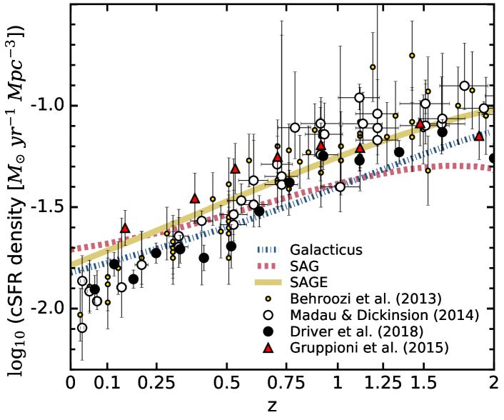
Figure 1: Cosmic star formation rate density of sag, sage and galacticus MultiDark-Galaxies as a function of redshift, compared to four independent compilations of data sets from Behroozi et al. (2013) (this was corrected to a Chabrier et al. (2014) IMF by the same authors), Madau & Dickinson (2014), Driver et al. (2018) and Gruppioni et al. (2015). The error bars are the 1$\sigma$ dispersion around each point. We show this result only up to $z\sim 2$, which is the maximum redshift of interest for our study.

2.1.4 Model comparison

For a full comparison between the sag, sage and galacticus semi-analytic models adopted in this work, we refer the reader to Knebe et al. (2018). The main differences between them are: i) the calibrations; ii) the treatment of mergers; iii) galaxies without a host halo, “orphans”, are not allowed in sage, while they can happen, due to mass stripping, within galacticus and sag; and iv) the metal enrichment models, with galacticus and sage assuming an instantaneous recycling approximation and sag implementing a more complete chemical model (Cora, 2006; Collacchioni et al., 2018).

Here we also recall some results from Knebe et al. (2018) that are important for interpreting the outcomes of our analysis and a further study of global properties can be found in Appendix C. As we impose a minimum limit of $M_{\star}\,$$>10^{8.87}\,$M_⊙ and SFR$\,>0\,\rm{yr^{-1}M_{\odot}}$ to the three SAMs of interest, some of our model results will be slightly different from those presented in Knebe et al. (2018). The cuts above have been chosen taking into account the resolution limit of the MultiDark cosmological simulation (see Knebe et al., 2018). At $z\sim 1$, the limit on SFR excludes about 4% of the entire sag population,  17% of galaxies in sage, and no galaxies from galacticus.

Fig. 1 shows the redshift evolution of the MultiDark-Galaxies cosmic star formation rate (SFR) density compared to a compilation of observations including estimates of the cosmic SFR from narrow-band (H$\alpha$), broad-band (UV-IR), and radio (1.4 GHz) surveys by Behroozi et al. (2013), and more recent results by Madau & Dickinson (2014), Gruppioni et al. (2015) and Driver et al. (2018). The observational data sets are consistent, despite being affected by different systematic errors. Fig. 1 only extends to $z\sim 2$, as higher redshifts are not of interest for this study. All the SAMs agree with the observations within our redshift range of interest $0.6<z<1.2$. Beyond $z=2$, sag and galacticus model galaxies maintain a good agreement with the data out to $z\sim 8.5$, while sage overpredicts the SFR density at $z\gtrsim 4$ (see Knebe et al., 2018).

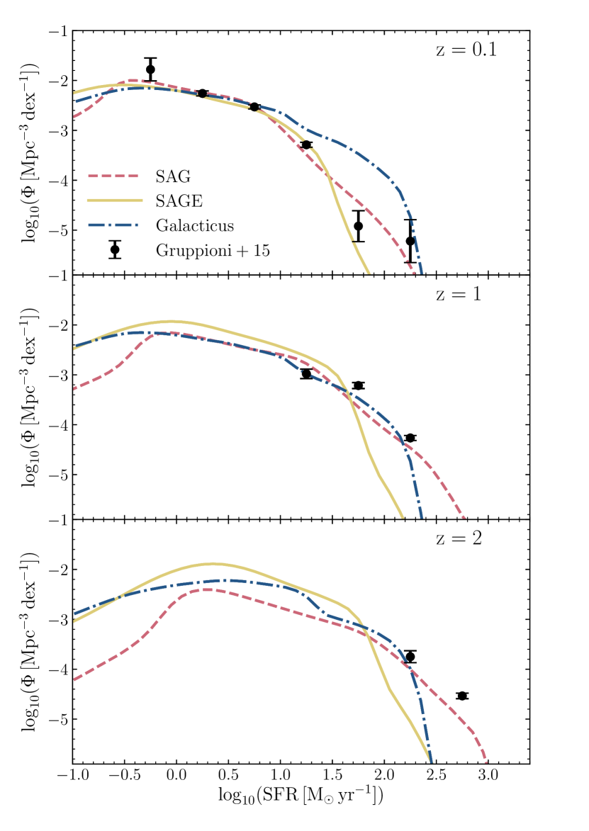
Figure 2: MultiDark-Galaxies average SFR function evolution at $z\lesssim 2$ (lines) compared to the Herschel/PEP and HerMES observations (Gruppioni et al., 2015, filled circles).

In SAMs, galaxy properties are obtained by solving coupled differential equations in a certain number of steps in which the time interval between snapshots of the underlying DM simulation is divided. In this context, we define the “instantaneous SFR” as the star formation rate computed using the mass of stars formed over the last step before the output. The “average SFR” is instead the SFR obtained by considering the average contribution from all the steps. The sag model subdivides the time between snapshots in 25. This timescale typically corresponds to $\sim$10-25 Myrs at $z\sim 1$, which is the timescale physically relevant for the $\left[\text{O\,{{ii}}}\right]$ emission. sage and galacticus split time in 10 steps.

Fig. 2 displays the average SFR functions of the MultiDark-Galaxies at different redshifts compared to the Herschel data from the PEP and HerMES surveys (Gruppioni et al., 2015). We find good agreement for SAG model galaxies over the whole SFR and $z$ ranges considered. galacticus is consistent with the measurements at $\rm{SFR}\lesssim 10^{2.5}\,$yr^-1M_⊙, while sage agrees with the data up to $10^{2}\,$yr^-1M_⊙. At higher SFRs, sage under-predicts the number of star-forming galaxies by $\sim 2$ dex.

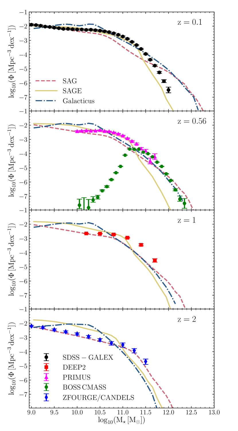
Figure 3: Stellar mass function evolution of our model galaxies (lines colour-coded as in the legend) compared to the SDSS-GALEX $z=0.1$ (Moustakas et al., 2013, black points) observations, the PRIMUS results at $0.50<z<0.65$ (Moustakas et al., 2013, magenta triangles), the BOSS CMASS measurements at $0.5<z<0.6$ not corrected from incompleteness (Maraston et al., 2013, green hexagons), the DEEP2-FF data at $0.9<z<1.1$ (red squares), and the ZFOURGE/CANDELS observations at $1.5<z<2.5$ (Tomczak et al., 2014, blue diamonds). Note that the BOSS data drop due to the selection of luminous, red, massive galaxies for this sample.

In Fig. 3, we show the evolution of the MultiDark-Galaxies stellar mass function compared to, from top to bottom, the SDSS-GALEX observations at $z=0.1$ (Moustakas et al., 2013), the PRIMUS measurements at $0.50<z<0.65$ (Moustakas et al., 2013), the BOSS CMASS observations at $0.5<z<0.6$ (Maraston et al., 2013), the DEEP2-FF data at $0.9<z<1.1$, and the ZFOURGE/CANDELS star-forming galaxies at $1.5<z<2.5$ (Tomczak et al., 2014). The BOSS CMASS mass function drops in the low-mass end due to the incompleteness effect generated by the CMASS colour cuts specifically designed to select luminous, red, massive galaxies (Maraston et al., 2013). Note that the stellar mass functions shown in Fig. 3 are not the same as those from Knebe et al. (2018) due to the SFR$>0$ cut we apply to the SAMs. The systematic errors on DEEP2 observations at $z\sim 1$ are expected to differ from those of SDSS galaxies at lower redshifts.

It is not surprising that the agreement between sag and ZFOURGE/CANDELS data is especially good because this model was calibrated against these observations. sage and galacticus over-predict the number of galaxies with $\rm{log(M_{\star}\,[M_{\odot}])\lesssim 11}$, and this excess is enhanced at higher redshift (from $\sim 0.1$ dex at $z=0.1$ to $\sim 0.4$ dex at $z=2$). sage under-estimates the number of galaxies more massive than $10^{11}$M_⊙ at all redshifts. We deem the MultiDark-Galaxies to be in sufficient agreement with observations in terms of their stellar-mass and SFR evolution such that we can draw meaningful predictions from the models that rely on these properties.

2.2 DEEP2 galaxies

We are interested in exploring the relationship between $L{\left[\mathrm{O\,\textrm{{{ii}}}}\right]}$ and different galactic properties. For comparison, we use an observational data set, the DEEP2–Firefly (DEEP2-FF, hereafter) galaxy sample, which allows us to test whether the model galaxies cover similar ranges of parameters, once the adequate selection functions are implemented.

The DEEP2 survey obtained spectra of about 50,000 galaxies brighter than $R\sim 24.1$, in four separate fields covering $\sim 2.8$ deg² (Newman et al., 2013). The redshift measurement for each object in the DEEP2 DR4 database was inspected by eye and assigned an integer quality code $-2<Q<4$ based on the determined accuracy of the redshift value. For this work, we consider galaxies with $Q>2$, corresponding to secure redshifts, within the range $0.001<z_{\rm{best}}<1.7$.

We adopt the DEEP2 flux-calibrated spectra generated by Comparat et al. (2016). We also use the extended photometric catalogues developed by Matthews et al. (2013), which supplement the DEEP2 photometric catalogues with ($u,g,r,i,z$) photometry from the Sloan Digital Sky Survey (SDSS). By applying the cuts specified above and taking into account the cross-match between the mentioned catalogues, the spectra of 33 838 galaxies from the original DEEP2 DR4 catalogue are used in this study. These spectra are fitted using stellar population models to extract quantities such as stellar masses, stellar metallicities, star formation rates, and ages. In particular, the DEEP2 SFR values are computed by fitting stellar population models to the spectral continuum, where the emission lines are masked for the fit. Thus, this constitutes an independent estimate from an $\left[\text{O\,{{ii}}}\right]$-based SFR.

The spectral fit is performed using the firefly code (Wilkinson et al., 2017; Comparat et al., 2017) in which no priors, other than the assumed model described immediately below, are applied. firefly treats dust attenuation in a novel way, by rectifying the continuum before the fit; for full details see Wilkinson et al. (2017) and Comparat et al. (2017). The firefly fit is performed for spectral templates with ages below 20 Gyr and metallicities in the range $0.001<Z<3$. The maximum age found for the DEEP2-FF sample is 10.18 Gyr. It is noteworthy to remark that firefly does not interpolate between the ages of the templates used in the spectral fitting. For this study, we adopt spectral templates from Maraston & Strömbäck (2011), assuming a Chabrier (2003) IMF, same as in the MultiDark-Galaxies, and the ELODIE stellar library. This latter covers the wavelength range $3900-6800$ Å with a 0.55 Å sampling at 5500 Å, i.e. at a resolution $R=10,000$ (Prugniel et al., 2007).

The DEEP2 survey used the DEIMOS spectrograph at Keck, which covers approximately the wavelength range $6500-9300$ Å  with a resolution $\sim\,$6000 (Faber et al., 2003). The discrepancy in wavelength coverage results in a lack of fits at low redshifts for this survey.

The firefly fits to the DEEP2 spectra described above are available at http://www.icg.port.ac.uk/Firefly/ (340 MB). Another fit to the DEEP2 spectra has been performed by Comparat et al. (2017) assuming slightly different age and metallicity ranges, and using a previous version of firefly that did not take into account the presence of mass loss in the stellar population models. Here we refer to “stellar mass” as the sum of the mass of living stars and the mass locked in stellar remnants (i.e., white dwarfs, neutron star and black holes).

2.2.1 Broad-band absolute magnitudes

The DEEP2-FF galaxy catalogue also provides SDSS $(u,g,r,i,z)$ apparent magnitudes. In order to compare these observations with the MultiDark-Galaxies absolute magnitudes, we have $(k+e)$ corrected them (where “$e$” stands for evolution). To this end, we have produced an evolving set of simple stellar populations (SSP; Maraston & Strömbäck, 2011) with ages, metallicities, and redshifts matching those used for the Firefly runs described above. In particular, we produce a table of possible evolutionary paths that provides the observed-frame properties of the given SSPs in the SDSS filters and allows us to determine the $k$-correction in those filters without any approximation. Hereafter, we will call it “MS table”. This table calculates intrinsic magnitudes. The DEEP2 data have been corrected from interstellar dust attenuation by applying Calzetti et al. (2000) extinction law.

These SDSS observed-frame properties are computed by red-shifting the model SEDs to a fixed grid of redshifts from $z=3.5$ down to $z=0.$, with $\Delta z=0.1$, and applying cosmological dimming using the Flexible-k-and-evolutionary-correction algorithm (FLAKE, Maraston, in prep.). We interpolate between the redshifts when needed. Such a technique has been widely used in the literature (e.g., Maraston et al., 2013; Etherington et al., 2017) and can be generalised to any arbitrary set of filters.

From each SSP model in the MS table above we extract the $(k+e)$ correction as:

$$(k+e)_{j}=M_{j}(z)-m_{j}=M_{j}(z)-M_{j}(z=0),$$ (1)

where $M_{j}(z)$ are the galaxy SDSS $j=(u,g,r,i,z)$ absolute magnitudes at redshift $z$ and $m$ are the observed magnitudes, i.e. the absolute magnitudes at $z=0$.

The Firefly spectral fitting code finds the best fit to a galaxy by weighting different SSPs and adding them together. It turns out that the best Firefly fits to the DEEP2 galaxy sample have only two SSP components. Thus, the DEEP2-FF galaxy sample can be cross-matched with the components of the MS table, by using a linear combination of the two SSP components of each Firefly (FF) best fit:

$${\rm{SSP}}^{\rm{MS}}=w_{0}\,{\rm{SSP}}_{0}^{\rm{FF}}+w_{1}\,{\rm{SSP}}_{1}^{\rm{FF}},$$ (2)

with $w_{0}+w_{1}=1$. Then, each DEEP2-FF galaxy is assigned a $(k+e)$ correction that is the weighted, linear combination of the corrections from each SSP component:

$$(k+e)_{j}=(k+e)_{j}^{0}\,w_{0}+(k+e)_{j}^{1}\,w_{1}.$$ (3)

2.2.2 The DEEP2–FIREFLY galaxy sample

For our analysis, we focus on DEEP2-FF galaxies within the redshift range $0.9<z<1.1$. We consider the sum of the $\left[\text{O\,{{ii}}}\right]$ 3727Å and 3729Å line fluxes as the $\left[\text{O\,{{ii}}}\right]$ doublet. Here we impose a flux limit of F${\left[\mathrm{O\,\textrm{{ii}}}\right]}$ $\,\rm{>5\,\sigma_{F_{[OII]}}}$ (where $\sigma_{F_{[OII]}}$ is the flux error) to guarantee robust flux estimates, and a minimum stellar mass uncertainty of $\rm{[\log_{10}(M_{\star}^{1\sigma\,up})-\log_{10}(M_{\star}^{1\sigma\,low})]/2<0.4}$. In the previous expression, $\rm{M_{\star}^{1\sigma\,up,low}}$ represents the Firefly stellar mass within $\pm 1\,\sigma$ from the mean value of the distribution.

After applying the cuts described above, our final sample includes 4478 emitters with minimum $\left[\text{O\,{{ii}}}\right]$ flux of $2.45\times 10^{-19}$ erg s^-1 cm^-2, mean $L{\left[\mathrm{O\,\textrm{{{ii}}}}\right]}$ $\sim 10^{41.6}$ erg s^-1, $M_{\star}\,$$\sim 10^{10.3}\,$M_⊙, age$\,\sim 10^{9.2}\,$yr, and mean cold gas metallicity $Z_{\rm{cold}}\sim 0.72$. Fig. 5 shows the distribution of $L{\left[\mathrm{O\,\textrm{{{ii}}}}\right]}$ as a function of SFR. The observed sample only populates a narrow range of SFR, and this affects the comparison with the model galaxies, which have SFRs lower than the minimum value of the DEEP2-FF sample. Other properties from this data set can be seen in Fig. 8 and in Appendix C. We assume the dust attenuation of the nebular emission lines to be the same as for the continuum. Thus, we also correct the $L{\left[\mathrm{O\,\textrm{{{ii}}}}\right]}$ from interstellar dust attenuation by applying Calzetti et al. (2000) extinction law, as we have detailed above for the broad-band magnitudes.

For the analysis, we select both observed and models galaxies using a more conservative flux cut, F${\left[\mathrm{O\,\textrm{{ii}}}\right]}$ $>5\times 10^{-18}$ erg s^-1 cm^-2. This corresponds to $L{\left[\mathrm{O\,\textrm{{{ii}}}}\right]}$ $\sim 10^{40.4}$ erg s^-1 at $z=1$ in Planck cosmology (Planck Collaboration et al., 2015), and roughly mimics the observational limitations (see also Gonzalez-Perez et al., 2018). This cut reduces the sparse, faint tail of the observed distribution (there are only 4 DEEP2 galaxies with flux lower than $5\times 10^{-18}$ erg s^-1 cm^-2) and allows us to obtain much narrower SAM constraints.

As shown in Fig. 4, most galaxies with $L{\left[\mathrm{O\,\textrm{{{ii}}}}\right]}$ $<10^{40.5}$ erg s^-1 have been removed from the DEEP2-FF sample, compared to the original DEEP2 population. Despite this, the DEEP2-FF galaxy sample is statistically representative of the original DEEP2 population. In fact, the cumulative distribution functions of these two samples, approximated by splines, differ by less than 5%, according to a Kolmogorov–Smirnov test.

Fig. 4 shows the distribution of the dust-attenuated $L{\left[\mathrm{O\,\textrm{{{ii}}}}\right]}$ computed with get_ emlines (see §3.1) from instantaneous and average SFRs, for SAG model galaxies at $z=0.94$ and with $M_{\star}\,$$>10^{8.87}{\rm M}_{\odot}$ and SFR$>0\,\rm{yr^{-1}M_{\odot}}$ (see Sec. 2.1.4). These model $L{\left[\mathrm{O\,\textrm{{{ii}}}}\right]}$ distributions are statistically different from the DEEP2-FF one. However, they have similar mean values: $\langle L{\left[\mathrm{O\,\textrm{{{ii}}}}\right]}\rangle\sim 10^{41}{\rm erg\,s^{-1}}$, $\langle\rm{age}\rangle\sim 10^{9.2}$yr, $\langle M_{\star}\rangle\sim 10^{9.47}{\rm M}_{\odot}$.

In order to draw a sample of model galaxies consistent with DEEP2-FF observations, we select sag galaxies with a $L{\left[\mathrm{O\,\textrm{{{ii}}}}\right]}$ distribution following the spline fit to the DEEP2-FF distribution, as shown in Fig. 4. We perform such a drawing for sag $\left[\text{O\,{{ii}}}\right]$ luminosities computed both from instantaneous and average SFR. The $L{\left[\mathrm{O\,\textrm{{{ii}}}}\right]}$ of these new selections have mean values consistent with those from the DEEP2-FF sample. Meanwhile, the ages, $\langle\rm{age}\rangle\sim 10^{9}$yr, and the stellar masses, $\langle M_{\star}\rangle\sim 10^{9.86}{\rm M}_{\odot}$, are lower than the observed ones.

In Appendix A, the DEEP2-FF sample is directly compared to the sag model galaxies selected following the DEEP2-FF $L{\left[\mathrm{O\,\textrm{{{ii}}}}\right]}$ distribution. These sag model subsets have brighter $L{\left[\mathrm{O\,\textrm{{{ii}}}}\right]}$, M_u and M_g values, slightly lower ages, higher stellar masses and span higher SFR values compared to the SAG selection at $M_{\star}\,$$>10^{8.87}{\rm M}_{\odot}$ and SFR$>0\,\rm{yr^{-1}M_{\odot}}$.

The main focus of this paper is to test the validity of different approaches for modelling emission lines in large galaxy samples with volumes comparable to the observable Universe. In this context, the comparison to the DEEP2-FF sample is meant to be a rough guide to the expected location of observed galaxies in different parameter spaces.

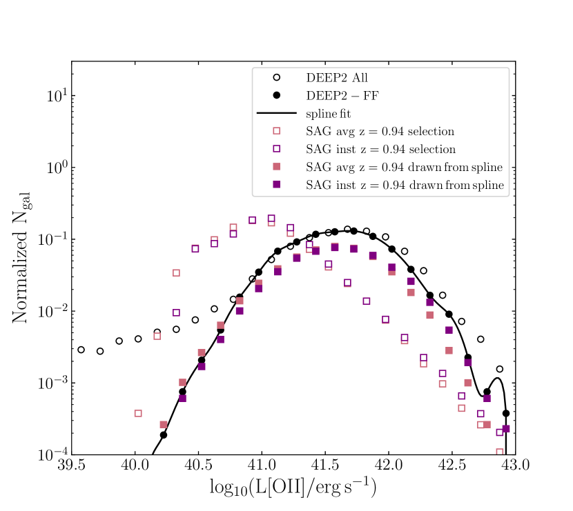
Figure 4: Attenuated $L{\left[\mathrm{O\,\textrm{{{ii}}}}\right]}$ distribution of the original DEEP2 sample (black, empty dots) compared to the DEEP2-FF selection (black, filled dots), which we fit with a spline function. The area under the curves is normalized to unity. We compare these results with the sag model galaxies selected with $M_{\star}\,$$>10^{8.87}{\rm M}_{\odot}$ and SFR$>0\,\rm{yr^{-1}M_{\odot}}$ (empty squares; see Sec. 2.1.4), and with the SAG galaxies randomly drawn from the DEEP2-FF spline distribution (filled squares). The $\left[\text{O\,{{ii}}}\right]$ luminosity values in the model galaxies are calculated using the get_ emlines code, inputing either the instantaneous (purple) or average (salmon) SFR. All the details about these quantities and the calculations are given in Sec. 3.1.

3 [Oii] emitters in the SAMs

The physics of $\left[\text{O\,{{ii}}}\right]$ emission lines is difficult to model, as it depends on local processes, such as dust extinction, and the inner structure and the ionising fields of the H ii nebula in which they are embedded. Different approaches have been used to model the $\left[\text{O\,{{ii}}}\right]$ emission line: (i) assume a relation between $L{\left[\mathrm{O\,\textrm{{{ii}}}}\right]}$ and SFR and, possibly, metallicity as it happens in observations (Kennicutt, 1998; Kewley et al., 2004; Moustakas et al., 2006; Jouvel et al., 2009; Sobral et al., 2012; Talia et al., 2015; Valentino et al., 2017); (ii) assume an average H ii region for a range of metallicities (Gonzalez-Perez et al., 2018); (iii) couple a photoionisation model with a galaxy evolution one (Hirschmann et al., 2012; Orsi et al., 2014). We address method (i) in Section 4 and method (iii) here.

None of the MultiDark-Galaxies catalogues studied in this work provides direct $L{\left[\mathrm{O\,\textrm{{{ii}}}}\right]}$ estimates. Therefore, we couple the SAMs with the get_ emlines model (Orsi et al., 2014), which encapsulates the results from the MAPPINGS-III photoionisation code (Groves et al., 2004; Allen et al., 2008). Here, the ionisation parameter of gas in galaxies is directly related to their cold gas metallicity, obtaining a reasonable agreement with the observed H$\alpha$, $\left[\mathrm{O\,\textrm{{{ii}}}}\right]\lambda 3727$, $\left[\mathrm{O\,\textrm{{{iii}}}}\right]\lambda 5007$ luminosity functions, and the Baldwin, Phillips & Terlevich (BPT; Baldwin et al., 1981) diagram for local star-forming galaxies. Ideally, the get_ emlines methodology requires as input the cold gas metallicity and the instantaneous SFR. This latter quantity, however, is not usually output by SAMs. The instantaneous SFR is preferred to a time-averaged equivalent, as the latter can include contributions from stellar populations older than those responsible for generating the nebular emission in star-forming galaxies.

sag is the only semi-analytic model providing both instantaneous and average SFR values, while sage and galacticus only provide average SFRs. In the next section, we describe in detail the get_ emlines algorithm to be used in the $L{\left[\mathrm{O\,\textrm{{{ii}}}}\right]}$ calculation for a semi-analytic model. Because SAMs do not usually output the instantaneous SFR, which is needed as default input for the get_ emlines code, we test the usage of the average SFR and how this affects different galactic properties.

3.1 The GET_ EMLINES code

We now describe step by step how we have implemented the get_ emlines nebular emission code to obtain $\left[\text{O\,{{ii}}}\right]$ luminosities for the MultiDark-Galaxies. This methodology is based on the photoionisation code MAPPINGS-III (Groves et al., 2004; Allen et al., 2008), which relates the ionisation parameter of gas in galaxies, $q$, to their cold gas metallicity $Z_{\rm{cold}}$ as:

$$q(Z)=q_{0}\left(\frac{Z_{\rm{cold}}}{Z_{0}}\right)^{-\gamma},$$ (4)

where $q_{0}$ is the ionisation parameter of a galaxy that has cold gas metallicity $Z_{0}$ and $\gamma$ is the exponent of the power law. Following Orsi et al. (2014), from the pre-computed H ii region model grid of Levesque et al. (2010), we assume $q_{0}=2.8\times 10^{7}\,\rm{cm\,s^{-1}}$, $Z_{0}=0.012$ and $\gamma=1.3$ for all the analysed galaxy models. This specific combination of values was presented in Orsi et al. (2014), and it has ionization parameter values that bracket the range spanned by the MAPPINGS-III grid for the bulk of the galaxy population studied in that work. The $q_{0}$ and $\gamma$ parameters above were found to produce model H$\alpha$, $\left[\mathrm{O\,\textrm{{{ii}}}}\right]\lambda 3727$ (to indicate the doublet), $\left[\mathrm{O\,\textrm{{{iii}}}}\right]\lambda 5007$ luminosity functions and a model BTP (Baldwin et al., 1981) diagram for local star-forming galaxies in good agreement with observations.

The get_ emlines code has been calibrated to reproduce a range of luminosity functions at different redshifts and local line ratios diagrams, and it has been tested against observations up to $z=5$ (Orsi et al., 2014). A different combination of $q_{0}$ and $\gamma$ changes the $L{\left[\mathrm{O\,\textrm{{{ii}}}}\right]}$ results in a complicated way. For instance, higher parameter values produce a lower number density of bright emitters, which translates into a substantial difference in the lower peak of the $L{\left[\mathrm{O\,\textrm{{{ii}}}}\right]}$-SFR bimodality shown in Fig. 5. Changing the $q_{0}$ and $\gamma$ parameters would require to recalibrate the get_ emlines model, and this goes beyond the scope of this work.

The cold gas metallicity is defined as the ratio between the cold gas mass in metals and the cold gas mass (e.g., Yates, 2014), considering both bulge and disc components, when available:

$$Z_{\rm{cold}}=\frac{M_{Z\rm{cold}}}{M_{\rm{cold}}}.$$ (5)

Another fundamental quantity needed to derive the $\left[\text{O\,{{ii}}}\right]$ line luminosity is the hydrogen ionising photon rate defined as:

$$Q_{\rm{H^{0}}}=\int_{0}^{\lambda_{0}}\frac{\lambda L_{\lambda}}{hc}d\lambda,$$ (6)

where $L_{\lambda}$ is the galaxy composite SED in erg s^-1 Å^-1, $\lambda_{0}=912$Å, $c$ is the speed of light and $h$ is the Planck constant. $Q_{\rm{H^{0}}}$ is a unit-less quantity calculated at each model snapshot just by solving the integral above. Assuming a Kroupa (2001) IMF, one can express the ionising photon rate as a function of the instantaneous star formation rate as Falcón-Barroso & Knapen (2013):

$$Q_{\rm{H^{0}}}=\rm{log_{10}1.35+log_{10}(SFR/M_{\odot}\,yr^{-1})+53.0.}$$ (7)

Combining Eq. 7 with the attenuation-corrected emission-line lists from Levesque et al. (2010), normalised to the H$\alpha$ line flux, we compute the $\left[\text{O\,{{ii}}}\right]$ luminosity as:

$$L(\lambda_{j})=1.37\times 10^{-12}Q_{\rm{H^{0}}}\frac{F(\lambda_{j},q,Z_{\rm{cold}})}{F(H\alpha,q,Z_{\rm{cold}})},$$ (8)

where $F(\lambda_{j},q,Z_{\rm{cold}})$ is the MAPPINGS-III prediction of the desired emission line flux at wavelength $\lambda_{j}$ for a given set of ($q$, $Z_{\rm{cold}}$) and $F(H\alpha,q,Z_{\rm{cold}})$ is the H$\alpha$ normalisation flux.

The total luminosity of the $\left[\text{O\,{{ii}}}\right]$ doublet is the sum of the luminosities of the two lines at $\lambda_{j}=3727,3729$ Å, both calculated using Eq. 8.

The $\left[\text{O\,{{ii}}}\right]$ luminosity in Eq. 8 does not include any dust contribution. In order to account for dust attenuation, we implement the correction detailed in next Section using Cardelli et al. (1989) extinction curve.

3.2 Dust extinction

In this study, the intrinsic $\left[\text{O\,{{ii}}}\right]$ luminosity given in Eq. 8, $L(\lambda_{j})$, is attenuated by interstellar dust as follows:

$$L(\lambda_{j})^{\rm{att}}=L(\lambda_{j})10^{-0.4A_{\lambda}(\tau_{\lambda}^{z},\theta)},$$ (9)

where $A_{\lambda}(\tau_{\lambda}^{z},\theta)$ represents the attenuation coefficient defined as a function of the galaxy optical depth $\tau_{\lambda}^{z}$ and the dust scattering angle $\theta$. Explicitly we have (Spitzer, 1978; Osterbrock, 1989; Draine, 2003; Izquierdo-Villalba et al., 2019):

$$A_{\lambda}(\tau_{\lambda}^{z},\theta)=-2.5\log_{10}\frac{1-\exp(-a_{\lambda}\,\sec\theta)}{a_{\lambda}\,\sec\theta},$$ (10)

where $a_{\lambda}=\sqrt{1-\omega_{\lambda}}\tau_{\lambda}^{z}$ and $\omega_{\lambda}$ is the dust albedo, i.e. the fraction of the extinction that is scattering. We assume $\cos\theta=0.60$ and $\omega_{\lambda}=0.80$, meaning that the scattering is not isotropic but more forward-oriented, and that 80% of the extinction is scattering. These are the values that return the best agreement with DEEP2+VVDS observations in Fig. 9.

The galaxy optical depth $\tau_{\lambda}^{z}$ that enters Eq. 10 is defined as (Devriendt et al., 1999; Hatton et al., 2003; De Lucia & Blaizot, 2007):

$$\tau_{\lambda}^{z}=\left(\frac{A_{\lambda}}{A_{V}}\right)_{Z_{\odot}}\left(\frac{Z_{\rm{cold}}}{Z_{\odot}}\right)^{s}\left(\frac{\langle N_{H}\rangle}{2.1\times 10^{21}\rm{atoms\,\,cm^{-2}}}\right),$$ (11)

where the first two factors on the right-hand side represent the extinction curve. This depends on the cold gas metallicity $Z_{\rm{cold}}$ defined in Eq. 5 according to power-law interpolations based on the solar neighbourhood, the Small and the Large Magellanic Clouds. The exponent $s=1.6$ (Guiderdoni & Rocca-Volmerange, 1987) holds for the $\lambda>2000$Å  regime, where the $\left[\text{O\,{{ii}}}\right]$ line is located. The $\left(A_{\lambda}/A_{V}\right)_{Z_{\odot}}$ term is the extinction curve for solar metallicity, which we take to be that of the Milky Way, and $\langle N_{H}\rangle$ the mean hydrogen column density. We adopt the values $Z_{\odot}=0.0134$ (Asplund et al., 2009) for the solar metallicity.

Assuming the Cardelli et al. (1989) extinction law in $0.3\,\mu\rm{m}\leq\lambda<0.9\,\mu\rm{m}$ (i.e., optical/NIR regime), one has:

$$\left(\frac{A_{\lambda}}{A_{V}}\right)=a(x)+b(x)/R_{V},$$ (12)

where $x\equiv\lambda^{-1}$, $R_{V}\equiv A_{V}/E(B-V)=3.1$ is the ratio of total to selective extinction for the diffuse interstellar medium in the Milky Way, and

$$a(x)= 1+0.17699\,y-0.50447\,y^{2}-0.02427\,y^{3}+$$ (13)

$$0.72085\,y^{4}+0.01979\,y^{5}-0.77530\,y^{6}+0.32999\,y^{7},$$

$$b(x)= 1.41338\,y+2.28305\,y^{2}+1.07233\,y^{3}-5.38434\,y^{4}$$

$$-0.62251\,y^{5}+5.30260\,y^{6}-2.09002\,y^{7},$$

with $y=(x-1.82)$.

The mean hydrogen column density is given by (Hatton et al., 2003; De Lucia & Blaizot, 2007):

$$\langle N_{H}\rangle=\frac{M_{\rm{cold}}^{\rm{disc}}}{1.4\,m_{p}\,\pi\,(a\,R_{1/2}^{\rm{disc}})^{2}}\,\,{\rm{atoms\,\,cm^{-2}}},$$ (14)

where $M_{\rm{cold}}^{\rm{disc}}$ is the cold gas mass of the disc, $m_{p}=1.67\times 10^{-27}\,{\rm{kg}}$ is the proton mass, $a=1.68$ is such that the column density represents the mass-weighted mean column density of the disc, and $R_{1/2}^{\rm{disc}}$ is the disc half-mass radius.

Qualitatively for this dust attenuation model, galaxies with large amounts of cold gas, metal rich cold gas and/or small scale sizes, will be the most attenuated ones (see also Merson et al., 2016).

3.3 Instantaneous versus average SFR

The get_ emlines code described in Section 3.1 ideally requires as inputs the instantaneous SFR and cold gas metallicity of galaxies. The instantaneous SFR, which is defined on a smaller time-step compared to the average SFR (see Sec. 2.1.4), traces very recent or ongoing episodes of star-formation, that are the relevant ones for nebular emission.

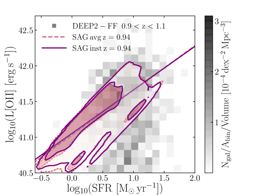
Figure 5: Intrinsic $\left[\text{O\,{{ii}}}\right]$ luminosity as a function of the SFR for the sag model galaxies at $z\sim 1$ (contours) and the DEEP2-FF observations at $0.9<z<1.1$ (grey, shaded squares). The bar represents the number density of DEEP2-FF galaxies in each 2D bin normalised by the bin area in units of [dex^-2 Mpc^-3]. We have imposed a minimum $\left[\text{O\,{{ii}}}\right]$ flux of 5$\times 10^{-18}$erg s^-1 cm^-2 to both observations and models. The model $L{\left[\mathrm{O\,\textrm{{{ii}}}}\right]}$ values are calculated by assuming instantaneous (solid, purple contours) and average (dashed, salmon) SFR as input for the get_ emlines prescription. The innermost (outermost) model contours encompass 68% (95%) percent of the galaxy distributions. The diagonal lines represent the $L{\left[\mathrm{O\,\textrm{{{ii}}}}\right]}$-SFR correlations, whose coefficients are given in Table 1.

Fig. 5 shows, as a function of SFR, the intrinsic (i.e. corrected from dust attenuation) $L{\left[\mathrm{O\,\textrm{{{ii}}}}\right]}$ that the coupling with get_ emlines gives for both the instantaneous (solid contours) and average (dashed) SFR from sag at $z\sim 1$. The innermost (outermost) contours enclose 68% (95%) of our model galaxies. The diagonal lines show the correlations between SFR and $L{\left[\mathrm{O\,\textrm{{{ii}}}}\right]}$. These are tight correlations, whose best-fitting parameters are reported in Table 1. Under laid are the DEEP2-FF observational data at $0.9<z<1.1$. Overall, the model galaxy distributions presented in Fig. 5 are very similar for the $L{\left[\mathrm{O\,\textrm{{{ii}}}}\right]}$ derived from either the instantaneous or the average SFRs. These distributions show a bimodality that can also be seen in the observations.

The instantaneous and average SFR derived distributions differ the most at SFR$\lesssim 10^{0}\,\rm{yr^{-1}M_{\odot}}$, with $\left[\text{O\,{{ii}}}\right]$ luminosities from average SFR being $\sim 0.2$ dex fainter than those from instantaneous SFR. At SFR$\sim 10^{1.5}$yr^-1M_⊙, there are slightly less bright $\left[\text{O\,{{ii}}}\right]$ emitters from instantaneous SFR.

DEEP2-FF galaxies in the upper density peak of the observed bimodal distribution shown in Fig. 5 are older, more massive, more luminous and slightly more star-forming (mean values: $\langle{\rm age}\rangle\sim 10^{9.28}$yr, $\langle$$M_{\star}\,$$\rangle\sim 10^{10.42}$M_⊙, $\langle$$L{\left[\mathrm{O\,\textrm{{{ii}}}}\right]}$ $\rangle\sim 10^{41.48}$erg s^-1, $\langle$SFR$\rangle\sim 10^{1.13}$yr^-1M_⊙) compared to their counterparts in the lower density area ($\sim 10^{9.13}$yr, $\sim 10^{10.22}$M_⊙, $\sim 10^{39.07}$erg s^-1, $\sim 10^{1.08}$yr^-1M_⊙). Overall, we find an opposite trend for model galaxies. In fact, the upper peak of the bimodality is composed of younger, less massive, slightly more luminous, less star-forming galaxies with mean values: $\langle$age$\rangle\sim 10^{9.16}$yr, $\langle$$M_{\star}\,$$\rangle\sim 10^{9.58}$M_⊙, $\langle$$L{\left[\mathrm{O\,\textrm{{{ii}}}}\right]}$ $\rangle\sim 10^{41.26}$erg s^-1, $\langle$SFR$\rangle\sim 10^{0.21}$yr^-1M_⊙); the lower peak has mean values: $\langle$age$\rangle\sim 10^{9.32}$yr, $\langle$$M_{\star}\,$$\rangle\sim 10^{10.06}$M_⊙, $\langle$$L{\left[\mathrm{O\,\textrm{{{ii}}}}\right]}$ $\rangle\sim 10^{41.25}$erg s^-1, $\langle$SFR$\rangle\sim 10^{0.83}$yr^-1M_⊙.

At the end of this Section, we will discuss further the origin of the DEEP2-FF $L{\left[\mathrm{O\,\textrm{{{ii}}}}\right]}$-SFR bimodal trend in connection with other galactic properties shown in Fig. 8.

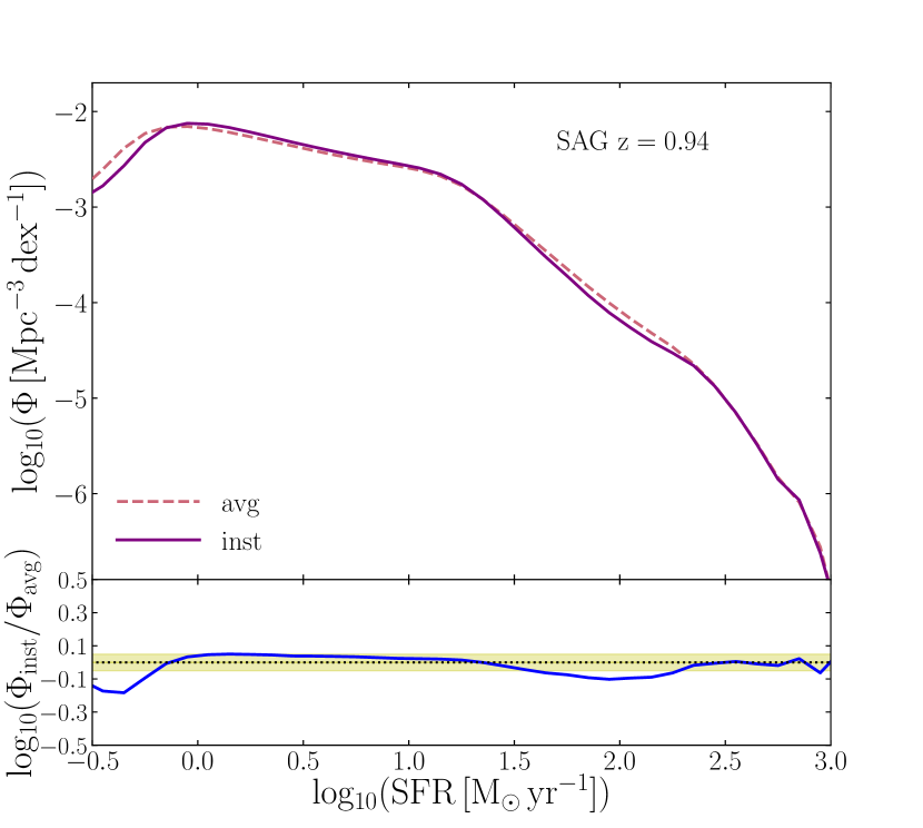
Figure 6: Average (dashed, salmon) versus instantaneous (solid, purple) SFR functions for SAG model galaxies. The bottom panel shows the ratio between the two, and the yellow, shaded region highlights the 5% region of agreement.

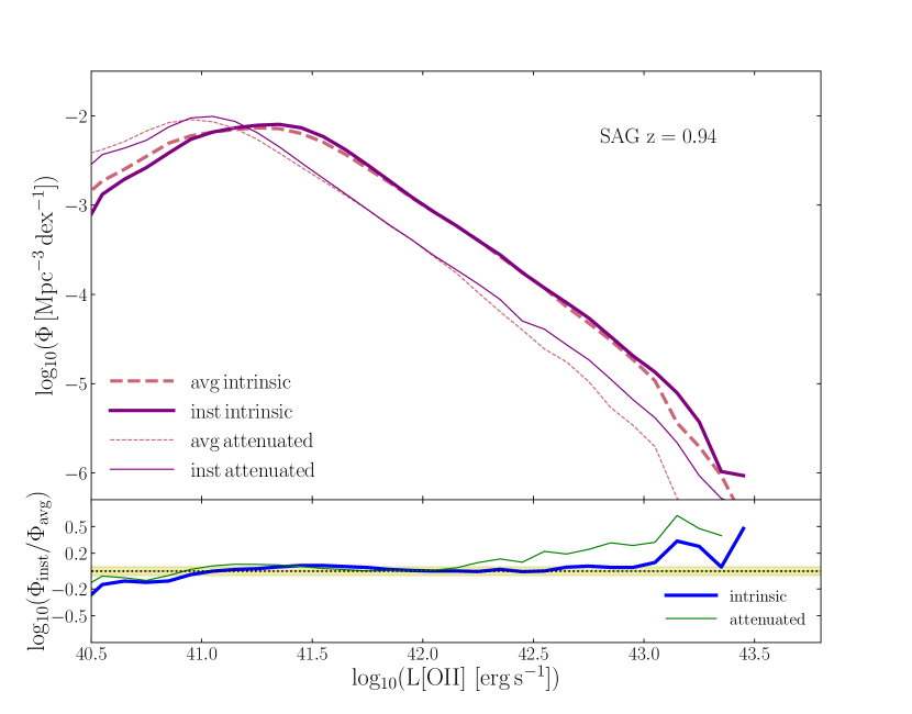
Figure 7: Intrinsic (thick lines) and attenuated (thin) $\left[\text{O\,{{ii}}}\right]$ luminosity functions based on sag average (dashed, salmon) and instantaneous SFR (solid, purple). The bottom panel shows the ratios between the two and the yellow stripe highlights the 5% region of agreement. We apply the mocks the same $\left[\text{O\,{{ii}}}\right]$ flux limit of DEEP2-FF observations, $5\times 10^{-18}$erg s^-1 cm^-2 (see Sec. 2.2.2).

In the top panel of Fig. 6 we compare the average (dashed, salmon) and instantaneous (solid, purple) sag SFR functions at $z\sim 1$, whose ratio is displayed in the bottom panel. The instantaneous and average SFR functions remain within 5% of each other at SFR$>10^{0}\,\rm{yr^{-1}M_{\odot}}$ (the 5% region is highlighted by the yellow shade). There is a slightly larger fraction, within 20%, of SAG galaxies having low average SFR, SFR$<10^{0}\,\rm{yr^{-1}M_{\odot}}$, than instantaneous values. The main difference between average and instantaneous SFRs is found for galaxies with the highest specific SFR (i.e., SFR/$M_{\star}\,$) and stellar masses below $10^{11}$M_⊙.

The top panel in Fig. 7 presents the intrinsic (thick lines) and attenuated (thin) $\left[\text{O\,{{ii}}}\right]$ luminosity functions derived from the average SFR (dashed, salmon line) and instantaneous SFR (solid, purple) from SAG. We impose on the sag model galaxies the same $\left[\text{O\,{{ii}}}\right]$ flux limit of DEEP2-FF observations, $5\times 10^{-18}$erg s^-1 cm^-2 (see Sec. 2.2.2), which corresponds to $L{\left[\mathrm{O\,\textrm{{{ii}}}}\right]}$ $\sim 10^{40.4}\,$erg s^-1 at $z=1$ in Planck cosmology (Planck Collaboration et al., 2015). The instantaneous-to-average amplitude ratios are displayed in the bottom panel of Fig. 7. The intrinsic (attenuated) $L{\left[\mathrm{O\,\textrm{{{ii}}}}\right]}$ functions have differences below 5% for luminosities in the range $10^{41}-10^{43}\,$erg s^-1 ($10^{41}-10^{42.2}\,$erg s^-1), which are highlighted by the yellow shade. At lower (higher) luminosities, the discrepancies grow up to 20% (30%). For the brightest galaxies, the discrepancy remains within 50%. The difference produced in $L{\left[\mathrm{O\,\textrm{{{ii}}}}\right]}$ by assuming average instead of instantaneous SFR does not change significantly with redshift over the range $0.6<z<1.2$ (see Appendix B for further details). Thus, the average and instantaneous SFR can be assumed interchangeably for average galaxies.

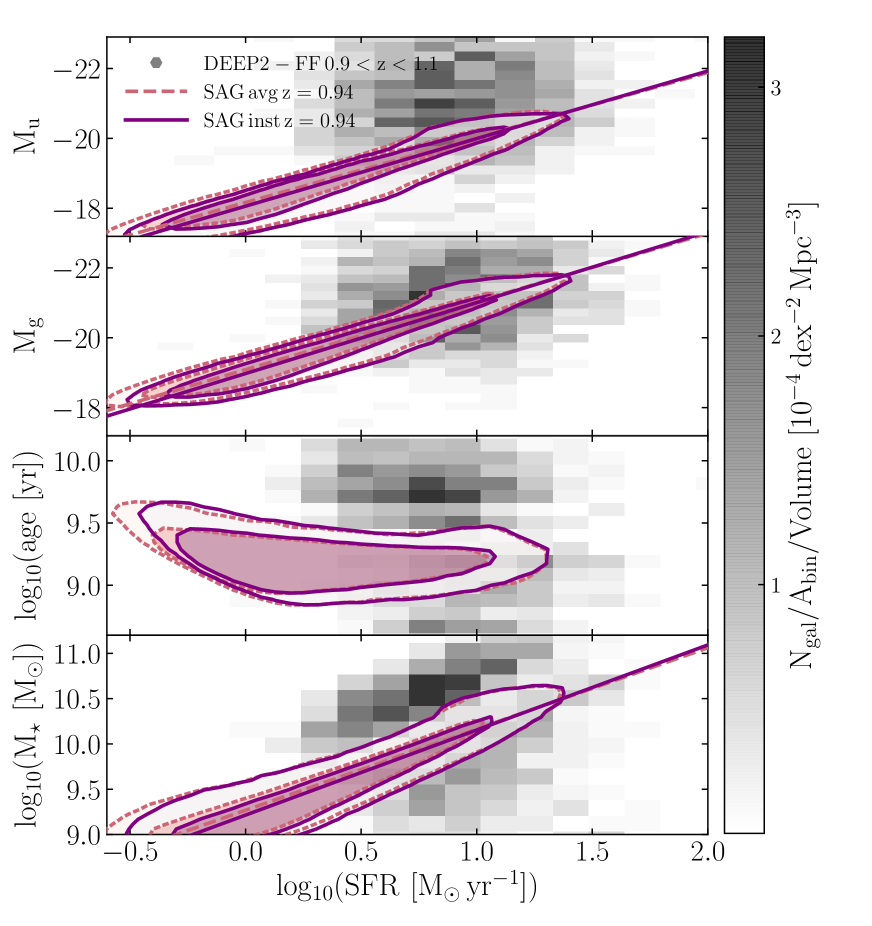
Figure 8: From top to bottom: intrinsic magnitudes, ages and stellar masses as a function of star formation rate for sag (contours) at $z\sim 1$ and DEEP2-FF observations at $0.9<z<1.1$ (grey, shaded squares). The colour bar shows the number density of DEEP2 galaxies per bin area in units of [dex^-2 Mpc^-3]. The dashed, salmon (solid, purple) contours represent the average (instantaneous) SFRs. The innermost (outermost) contours encompass 68% (95%) of the distributions. The diagonal lines are the linear fits showing the significant correlations (i.e. $r\geq 0.6$), whose coefficients are reported in Table 2, together with the best-fit parameters.

y=$A\,x+B$	$A$	$B$	$\sigma_{\rm y}$	$r$
y=log10($L{\left[\mathrm{O\,\textrm{{{ii}}}}\right]}$)
x=log${}_{10}({\rm SFR}_{\rm avg})$	0.625$\pm$0.001	41.03$\pm$0.01	0.40	0.83
x=log${}_{10}({\rm SFR}_{\rm inst})$	0.609$\pm$0.001	41.05$\pm$0.01	0.38	0.80
y=$M_{u}\,$
x=log${}_{10}({\rm SFR}_{\rm avg})$	-1.859$\pm$0.001	-18.17$\pm$0.01	1.07	0.92
x=log${}_{10}({\rm SFR}_{\rm inst})$	-1.934$\pm$0.001	-18.06$\pm$0.01	1.07	0.90
y=$M_{g}\,$
x=log${}_{10}({\rm SFR}_{\rm avg})$	-1.951$\pm$0.001	-19.09$\pm$0.01	1.11	0.93
x=log${}_{10}({\rm SFR}_{\rm inst})$	-2.029$\pm$0.001	-18.98$\pm$0.01	1.11	0.91
y=log${}_{10}($M${}_{\star})$
x=log${}_{10}({\rm SFR}_{\rm avg})$	0.897$\pm$0.001	9.27$\pm$0.01	0.54	0.89
x=log${}_{10}({\rm SFR}_{\rm inst})$	0.939$\pm$0.001	9.21$\pm$0.01	0.54	0.87

Table 1: Best-fit parameters of the linear scaling relations found for sag model galaxies at $z=1$ and shown in Fig. 8. The parameter $r$ is the correlation coefficient and $\sigma_{y}$ is the scatter in the $y$-axis. All the $L{\left[\mathrm{O\,\textrm{{{ii}}}}\right]}$ values are intrinsic.

In Fig. 8, from top to bottom, we display the sag broad-band $u$ and $g$ absolute magnitudes, ages and stellar masses as a function of the average SFR (dashed, salmon contour) and instantaneous SFR (solid, purple). We compare them with the DEEP2-FF observations at $0.9<z<11$ (grey, shaded squares). Except for the age, all these properties are tightly correlated with both SFRs. The lack of correlation between age and SFRs is clear for both the model and DEEP2-FF galaxies. We fit straight lines to the instantaneous and average contours and report the best-fit parameters and correlation coefficients in Table 1. For the broad-band magnitudes, the slopes of the average SFR correlations are only $\sim 0.07$ shallower than the instantaneous ones; for the stellar mass they are even closer. Overall, the width of the distributions as a function of both SFRs does not vary significantly. The average SFR contours extend down to slightly smaller values compared to the instantaneous contours.

The DEEP2-FF age and stellar mass distributions as a function of SFR in Fig. 8 show a bimodal trend, with an upper population of older, more massive, luminous, quiescent galaxies ($\langle\rm{age}\rangle\sim 10^{9.8}\,$yr, $\langle M_{\star}\rangle\sim 10^{10.82}\,{\rm M}_{\odot}$, $\langle$$L{\left[\mathrm{O\,\textrm{{{ii}}}}\right]}$ $\rangle\sim 10^{40.57}\,{\rm erg}\,{\rm s}^{-1}$, $\langle\rm{SFR}\rangle\sim 10^{1.02}\,{\rm yr}^{-1}{\rm M}_{\odot}$) and a lower tail of younger, less massive, luminous, more star-forming emitters ($\langle\rm{age}\rangle\sim 10^{8.48}\,$yr, $\langle M_{\star}\rangle\sim 10^{9.72}\,{\rm M}_{\odot}$, $\langle$$L{\left[\mathrm{O\,\textrm{{{ii}}}}\right]}$ $\rangle\sim 10^{40.45}\,{\rm erg}\,{\rm s}^{-1}$, $\langle\rm{SFR}\rangle\sim 10^{1.24}\,{\rm yr}^{-1}{\rm M}_{\odot}$). We obtain the same mean galaxy properties splitting the DEEP2-FF sample with a cut in either the age-SFR or Mstar-SFR planes.

The mean DEEP2-FF values derived from splitting in age or stellar mass as a function of SFR are similar to those obtained by splitting in $L{\left[\mathrm{O\,\textrm{{{ii}}}}\right]}$ versus SFR (see Fig. 5). The age/mass-SFR bimodal trend observed in DEEP2-FF galaxies is not reproduced by the SAG model galaxies, which instead look bimodal in the $L{\left[\mathrm{O\,\textrm{{{ii}}}}\right]}$-SFR plane (Fig. 5) because of the non-trivial dependence of $L{\left[\mathrm{O\,\textrm{{{ii}}}}\right]}$ on metallicity through the parameters $q_{0}$ and $\gamma$ (see Sec. 3.1).

In this section, we have shown that using the SAG average SFRs as input for the get_ emlines code gives results within 5% from using the instantaneous value for galaxies with attenuated $L{\left[\mathrm{O\,\textrm{{{ii}}}}\right]}$ in the range $10^{40.9}-10^{42.2}\,$erg s^-1, and with intrinsic $L{\left[\mathrm{O\,\textrm{{{ii}}}}\right]}$ between $10^{40.9}-10^{43}\,$erg s^-1. These are the ELGs with SFR within $10^{-0.2}-10^{1.6}\,$yr^-1 M_⊙. At higher and lower SFRs, there is a larger discrepancy between the average and instantaneous values, which translates into a larger difference ($<60\%$) in the number of bright $\left[\text{O\,{{ii}}}\right]$ emitters. Thus, this effect is not significant for the average galaxy population.

3.4 Model [Oii] luminosity functions

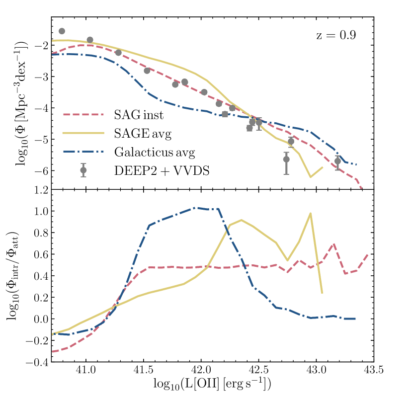
Figure 9: Top: Dust attenuated $\left[\text{O\,{{ii}}}\right]$ luminosity functions of the MultiDark-Galaxies at $z\sim 1$ compared with DEEP2+VVDS observations (Comparat et al., 2016). We consider all SAM galaxies above $5\times 10^{-18}$ erg s^-1 cm^-2. All the $\left[\text{O\,{{ii}}}\right]$ luminosities are computed using the get_ emlines code with SFR and cold gas metallicity as inputs (see Section 3.1). The SAG $L{\left[\mathrm{O\,\textrm{{{ii}}}}\right]}$, which are estimated using the instantaneous SFR, are in good agreement with the SAGE and Galacticus results based on the average SFR. Bottom: Ratios between the model intrinsic $\left[\text{O\,{{ii}}}\right]$ luminosity functions (given by Eq. 8) and the dust attenuated ones (see Sec. 3.2) shown in the upper panel.

In the top panel of Fig. 9, we present the MultiDark-Galaxies dust attenuated $\left[\text{O\,{{ii}}}\right]$ luminosity functions at $z=0.94$ compared to a compilation of DEEP2 and VVDS data from Comparat et al. (2016). Note that similar results have been found within the redshift range $0.6<z<1.2$, although they are not shown here. The SAM $\left[\text{O\,{{ii}}}\right]$ luminosities have been derived using the get_ emlines code described above coupled with instantaneous SFR for SAG model galaxies, and average SFR for SAGE and Galacticus, for which the instantaneous quantity is not available. The dust attenuation has been accounted for by correcting these luminosities applying Eq. 9 with Cardelli et al. (1989) extinction curve. There are varying degrees of agreement between the models and observational data across the $\sim$3 decades in $\left[\text{O\,{{ii}}}\right]$ luminosity and redshift range considered. Nevertheless, the trends from all the data sources are consistent. This plot highlights that the shape and normalisation of a predicted $\left[\text{O\,{{ii}}}\right]$ luminosity function from a SAM are robust to both the precise prescriptions that govern galaxy evolution in the model, and the calculation of $\left[\text{O\,{{ii}}}\right]$ from either instantaneous or average SFR.

In the top panel of Fig. 9, we see a drop in the number of Galacticus $\left[\text{O\,{{ii}}}\right]$ emitters at intermediate luminosities that is independent of the stellar mass. This is mainly determined by the half mass radii of the disc, R${}_{1/2}^{\rm disc}$, that enter the dust attenuation correction (see Eq. 14). These radii in Galacticus are about 50% smaller than in SAG and SAGE. At $L{\left[\mathrm{O\,\textrm{{{ii}}}}\right]}$ $\gtrsim 10^{42.5}$erg s^-1 and $z<1.2$, Galacticus predicts about 0.5 dex more $\left[\text{O\,{{ii}}}\right]$ emitters than the other two models.

In the bottom panel of Fig. 9, we display the ratios of the attenuated-to-intrinsic $L{\left[\mathrm{O\,\textrm{{{ii}}}}\right]}$ functions. As expected, the largest effect of attenuation occurs at $L{\left[\mathrm{O\,\textrm{{{ii}}}}\right]}$ $\gtrsim 10^{42}\,$erg s^-1, where more massive galaxies are located, while in the low-luminosity, low-mass regime, the observed and intrinsic signals tend to overlap. The ratio between the intrinsic and attenuated luminosity functions is model dependent. In particular, the largest variations are due to the dust model, which depends on the metallicity, gas content and size of each galaxy, as described in § 3.2. For sage model galaxies, this ratio increases for brighter $L{\left[\mathrm{O\,\textrm{{{ii}}}}\right]}$ galaxies. For sag, the ratio also increases up to $L{\left[\mathrm{O\,\textrm{{{ii}}}}\right]}$ $\gtrsim 10^{41.5}\,$erg s^-1, although with a steeper slope, and beyond this value it reaches a plateau. The ratio for galacticus has a prominent bump in the luminosity range $10^{41.5}-10^{42.5}\,$erg s^-1, where the effect of attenuation is more pronounced, and this feature corresponds to the drop seen at intermediate $L{\left[\mathrm{O\,\textrm{{{ii}}}}\right]}$ in the upper panel. At higher luminosities, there is almost no difference between the intrinsic and dust attenuated galacticus $L{\left[\mathrm{O\,\textrm{{{ii}}}}\right]}$ functions.

4 [Oii] luminosity proxies

Observational studies have shown tight correlations between the $\left[\text{O\,{{ii}}}\right]$ luminosity, SFR (Kennicutt, 1998; Sobral et al., 2012; Kewley et al., 2004; Moustakas et al., 2006; Comparat et al., 2015) and the galaxy UV-emission (Comparat et al., 2015), without the need to introduce any dependence on metallicity (Moustakas et al., 2006). This has prompted authors of theoretical papers to treat star-forming galaxies as ELGs when making predictions for upcoming surveys (e.g. Orsi & Angulo, 2018; Jiménez et al., 2019).

Here we explore the possibility of using simple, linear relations to infer the $\left[\text{O\,{{ii}}}\right]$ luminosity from global galaxy properties that are commonly output in SAMs. For this purpose, we investigate both observationally motivated prescriptions (Section 4.1), and we derive model relations from the get_ emlines code coupled with the SAMs considered (Sections 4.2 and 4.3). For this last study, we quantify the correlation between the model $L{\left[\mathrm{O\,\textrm{{{ii}}}}\right]}$ from get_ emlines with the average SFR, broad-band magnitudes, stellar masses, ages and cold gas metallicities. Directly using the measured $L{\left[\mathrm{O\,\textrm{{{ii}}}}\right]}$-SFR linear relation is useful to understand when is adequate to consider ELGs equivalent to star-forming galaxies and when it is not.

We find that the stellar mass of the MultiDark-Galaxies are unaffected by the change in proxies for estimating their $\left[\text{O\,{{ii}}}\right]$ luminosities. As a consequence, the stellar-to-halo mass relation (SHMR) is also unchanged using different $L{\left[\mathrm{O\,\textrm{{{ii}}}}\right]}$ proxies.

We remind the reader that, unless otherwise specified, we exclusively select emission line galaxies with fluxes above $5\times 10^{-18}\rm{erg\,s^{-1}\,cm^{-2}}$ in both the DEEP2-FF observations and MultiDark-Galaxies. This flux limit corresponds to a $L{\left[\mathrm{O\,\textrm{{{ii}}}}\right]}$ $>10^{40.4}\,$erg s^-1 at $z=1$ in the Planck cosmology (Planck Collaboration et al., 2015). All the results in what follows have these minimum cuts applied.

4.1 The SFR–L[Oii] relation

In this Section, we derive intrinsic $L{\left[\mathrm{O\,\textrm{{{ii}}}}\right]}$ from the average SFR of the MultiDark-Galaxies using three different, published relations assuming a Kennicutt (1998) IMF. These are: the Moustakas et al. (2006) conversion (see also Comparat et al., 2015) calibrated at $z=0.1$,

$$\rm{L_{[OII]}^{Moust}}({\rm{erg}\,\,s}^{-1})=\frac{SFR({\rm{M}}_{\odot}\,{\rm{yr}}^{-1})}{2.18\times 10^{-41}},$$ (15)

the Sobral et al. (2012) formulation optimised at $z=1.47$,

$$\rm{L_{[OII]}^{Sob}}({\rm{erg}\,\,s}^{-1})=\frac{SFR({\rm{M}}_{\odot}\,{\rm{yr}}^{-1})}{1.4\times 10^{-41}},$$ (16)

the Kewley et al. (2004) conversion calibrated at $z=1$,

$$\rm{L_{[OII]}^{Kew}}(erg\,s^{-1})=\frac{SFR({\rm{M}}_{\odot}\,{\rm{yr}}^{-1})}{7.9\times 10^{-42}}$$ (17)

$$\times(a[12+\log_{10}({\rm{O/H}})_{\rm{cold}}]+b).$$

The coefficients $(a,b)$ in the equation above are the values from Kewley et al. (2004) derived for the $R_{23}$ metallicity diagnostic (Pagel et al., 1979). The $[12+\log_{10}(\rm{O/H})_{\rm{cold}}]$ term is the $\left[\text{O\,{{ii}}}\right]$ ELG gas-phase oxygen abundance, which we proxy with the cold gas-phase metallicity $Z_{\rm{cold}}$ given in Eq. 5 through the solar abundance and metallicity. Explicitly we have:

$${12+\log_{10}{\rm{(O/H)_{cold}}}}=[{12+\log_{10}{\rm{(O/H)_{\odot}}}}]\frac{Z_{\rm{cold}}}{Z_{\odot}},$$ (18)

where we assume $Z_{\odot}=0.0134$ (Asplund et al., 2009), and $[12+\log_{10}{\rm(O/H)_{\odot}}]=8.69$ (Allende Prieto et al., 2001). As the above relations are for intrinsic luminosities, dust attenuated quantities are obtained following the description in § 3.2.

For sag and galacticus, galaxies’ cold gas is broken into bulge and disc components (see their respective papers for their definitions of a ‘gas bulge’); we therefore take a mass-weighted average of these components’ metallicities to obtain $Z_{\rm cold}$. sage instead always treats cold gas as being in a disc. In addition, the sag catalogues also output the $\rm{(O/H)_{cold}}$ values, which are mass density ratios, that we use in the calculation of Eq. 17 for sag model galaxies. In order to derive the correct abundances in terms of number densities, we need to rescale them by the Oxygen-to-Hydrogen atomic weight ratio, $A_{\rm{O}}/A_{\rm{H}}\sim 15.87$.

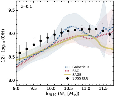
Figure 10: Mean gas-phase oxygen abundance in bins of stellar mass of the SDSS emission line galaxies at $z\sim 0.1$ (Favole et al., 2017) compared to the MultiDark-Galaxies models. The abundance is computed for the SAMs using Eq. 18. The error bars on the SDSS measurements are the $1\sigma$ scatter around the mean.

Fig. 10 displays the comparison between the gas-phase oxygen abundances of our SAM galaxies computed using Eq. 18 and the observed abundance of the SDSS $\left[\text{O\,{{ii}}}\right]$ ELGs at $z\sim 0.1$ from Favole et al. (2017). The SDSS metallicity values have been derived from the MPA-JHU DR7 catalogue of spectrum measurements and are built according to the works of Tremonti et al. (2004) and Brinchmann et al. (2004). Overall, we find that the gas-phase oxygen abundance in MultiDark-Galaxies increases with stellar mass up to $M_{\star}\,$$\sim 10^{11}\,$M_⊙. Beyond this value it drops and reaches a plateau.

The sag and sage model galaxies under-predict the gas-phase oxygen abundance by an average factor of $\sim 0.02\,$dex. This systematic offset for SAGE is not predictive, but purely due to the fact that this model was calibrated by assuming a different value of ${\rm{(O/H)}}_{\odot}/Z_{\odot}$, specifically ${\rm{[12+log_{10}(O/H)]=[9+log_{10}}}(Z_{\rm{cold}}/0.02)]$; for further details, see Knebe et al. (2018).

At $M_{\star}\,$$<10^{10.2}\,$M_⊙, galacticus also under-predicts the gas-phase abundance by the same factor. However, this model exhibits a bump at $M_{\star}\,$$\sim 10^{10.5}\,$M_⊙. This feature is related to the excess of galaxies around this stellar mass, which is seen in the galaxy stellar mass function (see Fig. 3). This excess was found to be produced by the depletion of gas due to the extreme AGN feedback mechanism implemented in galacticus, where the galaxies have almost no inflow of pristine gas, and rapidly consume their gas supply (for further details, see Knebe et al., 2018).

We have investigated further this feature finding that, if we exclude galaxies with progressively higher cold gas fraction (CGF), which is defined as CGF=$M_{\rm{cold}}$/$M_{\star}$, the bump shrinks continuously. Fig. 10 is produced by combining two cuts: CGF$>0.1$ and sSFR$>10^{-11}\,$yr^-1. The first one eliminates about half of the galacticus model galaxies, most of them with unrealistically small CGFs, possibly meaning that their metallicities are not reliable due to the precision used in evolving the relevant ordinary differential equations (Benson, 2012). The second cut selects only very star-forming galaxies. The bump completely disappears for CGF$>0.5$, but in that case $\sim 70\%$ of the galaxies are excluded from the sample.

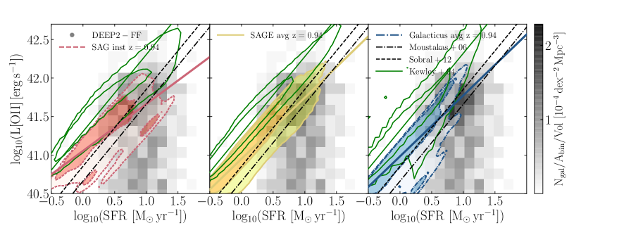
Figure 11: Intrinsic $\left[\text{O\,{{ii}}}\right]$ luminosity as a function of the SFR from the MultiDark-Galaxies at $z\sim 1$ (salmon, yellow and blue, filled contours), compared with the DEEP2-FF observations at $0.9<z<1.1$ (grey, shaded squares, colour-coded with the density of emitters per 2D bin area). The innermost (outermost) contour represents 68% (95%) of the galaxy distributions. For sag model galaxies, the $\left[\text{O\,{{ii}}}\right]$ luminosities have been computed from instantaneous SFRs, while for the other SAMs they are based on average SFRs. Both data and model ELGs are selected imposing a minimum $\left[\text{O\,{{ii}}}\right]$ flux of 5$\times 10^{-18}$ erg s^-1 cm^-2. The thick, coloured, diagonal lines are the linear fits to each SAM distribution, and their best-fit parameters are reported in Table 2. The black dot-dashed and dashed, diagonal lines are the $L{\left[\mathrm{O\,\textrm{{{ii}}}}\right]}$ predictions obtained from the SFR range of interest using Eqs. 15 and 16, respectively. The green, empty contours are the Kewley et al. (2004) predictions obtained using Eq. 17 with SFR and cold gas metallicity as inputs. The green, solid lines are the same predictions assuming median metallicity values in bins of SFR.

Fig. 11 compares the intrinsic $\left[\text{O\,{{ii}}}\right]$ luminosity as a function of SFR for the three SAMs (coloured, filled contours) with the DEEP2-FF data at $z\sim 1$ (grey, shaded squares). We also show the results of the conversions given in Eqs. 15-17 (diagonal, black and green lines). The model $L{\left[\mathrm{O\,\textrm{{{ii}}}}\right]}$ is computed using the get_ emlines code coupled with instantaneous SFR for SAG, and average SFR for the other semi-analytic models. The distributions of sag, sage and galacticus behave in a similar way, reproducing the bimodality observed in the data. The coloured lines (dashed, salmon; solid, yellow; dot-dashed, blue) are the linear fits to the model $L{\left[\mathrm{O\,\textrm{{{ii}}}}\right]}$-SFR correlations. The best-fit parameters, correlation coefficients ($r$-values) and dispersions in both directions are reported in Table 2.

Fig. 11 shows that all the model galaxies considered overlap with the DEEP2-FF observations and extend further towards lower SFR values. All three SAMs cover the $L{\left[\mathrm{O\,\textrm{{{ii}}}}\right]}$ observational range with their $2\sigma$ regions. sage and galacticus get to the very bright domain of the parameter space, while sag is limited to fainter $L{\left[\mathrm{O\,\textrm{{{ii}}}}\right]}$ values.

All the SAMs are tightly correlated in the SFR–luminosity plane and such a trend is in reasonable agreement with the observationally derived relations from Eqs. 15-17 (diagonal, black and green lines).

In Fig. 11, the Kewley et al. (2004) parametrisation (green line and contours in Fig. 11) appears above all the get_ emlines derivations. These contours are obtained from Eq. 17, by inputting instantaneous (average) SFR and cold gas metallicity for sag (sage, galacticus) model galaxies. The green, straight lines are calculated by feeding the median metallicity values in bins of SFR into Eq. 17. Although both the Kewley et al. (2004) relation and the get_ emlines code assume the same cold gas metallicity values as inputs, the obtained distributions are very different. The width of the distributions is model-dependent and the $L{\left[\mathrm{O\,\textrm{{{ii}}}}\right]}$ obtained for galaxies in sag and Galacticus present bimodal distributions. This bimodality comes from the MAPPINGS-III term $F(\lambda_{j},q,Z_{\rm{cold}})$ in Eq. 8, that is a non-linear function of $Z_{\rm{cold}}$.

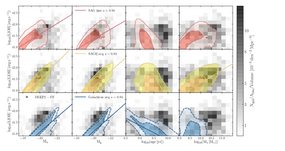
Figure 12: From top to bottom and from left to right: sag, sage and galacticus $z\sim 1$ intrinsic $\left[\text{O\,{{ii}}}\right]$ luminosities versus broad-band magnitudes, ages and stellar masses (contours) compared with the DEEP2-FF observations at $0.9<z<1.1$ (grey, shaded squares). The $L{\left[\mathrm{O\,\textrm{{{ii}}}}\right]}$ values are computed using the get_ emlines code with instantaneous SFR for sag and average SFR for sage and galacticus. The innermost and outermost model contours represent 68% ($1\sigma$) and 95% ($2\sigma$) of the distribution. A minimum $\left[\text{O\,{{ii}}}\right]$ flux cut of $\rm{5\times 10^{-18}\,\,erg\,s^{-1}\,cm^{-2}}$ has been applied to both data and model galaxies. The diagonal lines are the linear fits for strong correlations with $r>0.6$, as reported in Table 2.

z=1		sag	sage	galacticus
log${}_{10}(L{\left[\mathrm{O\,\textrm{{{ii}}}}\right]/\rm{erg\,s^{-1}}}$)  = $A$ log10(SFR/M⊙ yr-1)+$B$	$A$	0.609$\pm$0.001	0.792$\pm$0.001	0.795$\pm$0.001
	$B$	41.05$\pm$0.01	40.98$\pm$0.01	40.95$\pm$0.01
	$\sigma_{\rm{\log(SFR)}}$	0.50	0.53	0.48
	$\sigma_{\rm{\log(L[OII])}}$	0.38	0.45	0.46
	$r$	0.80	0.92	0.83
log${}_{10}(L{\left[\mathrm{O\,\textrm{{{ii}}}}\right]/\rm{erg\,s^{-1}}}$)  = $A$ $M_{u}\,$+$B$	$A$	-0.231$\pm$0.001	-0.373$\pm$0.001	-0.323$\pm$0.001
	$B$	36.93$\pm$0.01	34.01$\pm$0.01	34.61$\pm$0.01
	$\sigma_{\rm{M_{u}}}$	1.07	1.05	1.18
	$\sigma_{\rm{\log(L[OII])}}$	0.38	0.45	0.46
	$r$	0.65	0.86	0.83
log${}_{10}(L{\left[\mathrm{O\,\textrm{{{ii}}}}\right]/\rm{erg\,s^{-1}}}$)  = $A$ $M_{g}\,$+$B$	$A$	-0.218$\pm$0.001	-0.342$\pm$0.001	-0.328$\pm$0.001
	$B$	36.97$\pm$0.01	34.29$\pm$0.01	34.53$\pm$0.01
	$\sigma_{\rm{M_{g}}}$	1.11	1.08	1.15
	$\sigma_{\rm{\log(L[OII])}}$	0.38	0.45	0.46
	$r$	0.64	0.81	0.82
log${}_{10}(L{\left[\mathrm{O\,\textrm{{{ii}}}}\right]/\rm{erg\,s^{-1}}}$)  = $A$ log(age/yr)+$B$	$A$	—	—	-0.646$\pm$0.001
	$B$	—	—	47.17$\pm$0.01
	$\sigma_{\rm{\log(age)}}$	—	—	0.54
	$\sigma_{\rm{\log(L[OII])}}$	—	—	0.46
	$r$	-0.44	-0.47	-0.76
log${}_{10}(L{\left[\mathrm{O\,\textrm{{{ii}}}}\right]/\rm{erg\,s^{-1}}}$)  = $A$ log($M_{\star}\,$/M⊙)+$B$	$A$	—	0.563$\pm$0.001	—
	$B$	—	35.70$\pm$0.01	—
	$\sigma_{\rm{log(M\star)}}$	—	0.52	—
	$\sigma_{\rm{log(L[OII])}}$	—	0.45	—
	$r$	0.54	0.64	0.03

Table 2: Best-fit parameters of the linear scaling relations shown in Figs. 11 and 12. All the $\left[\text{O\,{{ii}}}\right]$ luminosities here are intrinsic and computed using the get_ emlines code with input the instantaneous SFR for sage and average SFR for sage and galacticus.

4.2 L[Oii] versus broad-band magnitudes

At a given redshift range, the broad-band magnitudes tracing the rest-frame UV emission of a galaxy are expected to be tightly correlated with the SFR and the production of emission line galaxies. The rest-frame UV slope ($1000-3000$ Å) at $z\sim 1$ is measured between the $u$ and the $g-$bands ($\sim 2000$Å). As expected, these are the bands that correlate the most with both SFR and $\left[\text{O\,{{ii}}}\right]$ luminosity for the sample under study.

The correlations between the broad-band $u$ and $g$ absolute magnitudes and the intrinsic $\left[\text{O\,{{ii}}}\right]$ luminosity in MultiDark-Galaxies at $z\sim 1$ are displayed in the first two columns of panels in Fig. 12 together with DEEP2-FF observations. Data and all model galaxies show a good overlap in this parameter space. The observations populate a smaller region of the parameter space, while the SAMs extend down to lower SFR and $L{\left[\mathrm{O\,\textrm{{{ii}}}}\right]}$ values. We over plot all the strong correlations (i.e. those with correlation coefficient $r\geq 0.6$) as linear scaling laws with an associated scatter $\sigma_{\rm{y}}$. Their best-fit parameters ($A,\,B$) and correlation coefficients ($r$) can be found in Table 2, where relations with $r<0.6$ have been omitted. We find both the $u$ and $g$ magnitudes to be tightly correlated with $L{\left[\mathrm{O\,\textrm{{{ii}}}}\right]}$, and thus they have the potential to be used as proxies for the $\left[\text{O\,{{ii}}}\right]$ luminosity, using the relations presented in Table  2.

4.3 L[Oii] versus age, metallicity and stellar mass

We also study the dependence of the $\left[\text{O\,{{ii}}}\right]$ luminosity on galaxy properties that are relevant to the $L{\left[\mathrm{O\,\textrm{{{ii}}}}\right]}$ and $(k+e)$ calculations: the age, metallicity, and stellar mass.

The right column of panels in Fig. 12 shows the relationship between the intrinsic $\left[\text{O\,{{ii}}}\right]$ luminosity and the stellar mass in both DEEP2-FF and our model galaxies. In sage we identify a correlation, but none is found for sag and galacticus model galaxies. The DEEP2-FF data do not exhibit any particular trend, maybe due to the narrow luminosity range that the sample covers.

In the third column of Fig. 12, we display the relationship between the intrinsic $L{\left[\mathrm{O\,\textrm{{{ii}}}}\right]}$ and age, which is mostly flat both in MultiDark-Galaxies and DEEP2-FF observations, with the latter showing a bimodal distribution. Only galacticus model galaxies exhibit an anti-correlation in the age-$L{\left[\mathrm{O\,\textrm{{{ii}}}}\right]}$ plane.

No correlation is found between the metallicity and $L{\left[\mathrm{O\,\textrm{{{ii}}}}\right]}$ for any of the models (this is not shown in Fig. 12). We conclude that none of the galaxy properties explored in this Section are good candidates as proxies for $L{\left[\mathrm{O\,\textrm{{{ii}}}}\right]}$.

4.4 From galaxy properties to L[Oii]

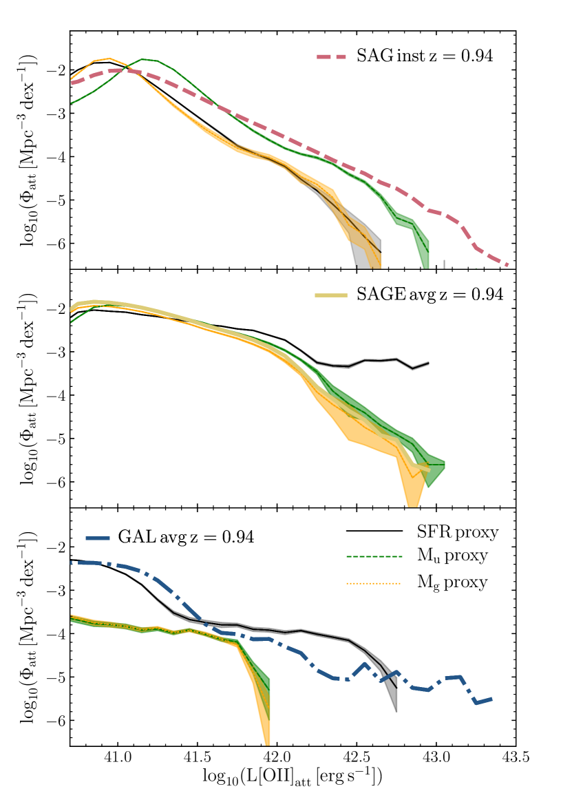
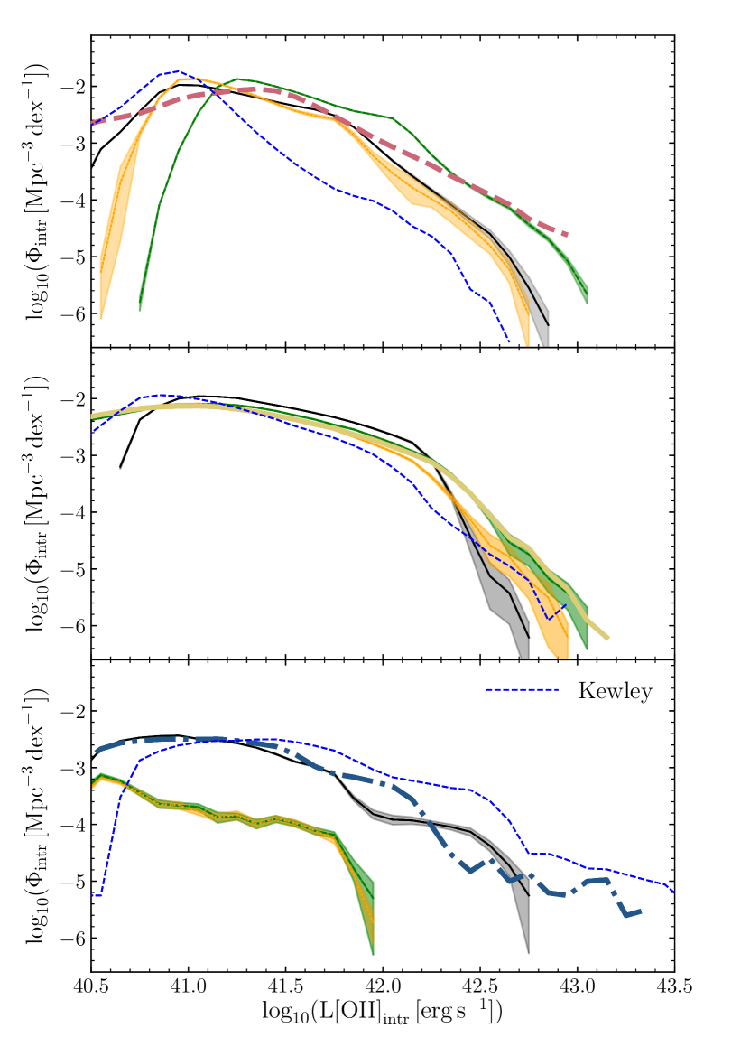
Figure 13: Left column: From top to bottom, attenuated $\left[\text{O\,{{ii}}}\right]$ luminosity functions of the sag, sage and galacticus model galaxies at $z\sim 1$. We show as thick lines the results with $L{\left[\mathrm{O\,\textrm{{{ii}}}}\right]}$ computed using the get_ emlines code described in Section 3.1 with either instantaneous or average SFR and metallicity as inputs. We compare these results with the $L{\left[\mathrm{O\,\textrm{{{ii}}}}\right]}$ functions derived from the three $L{\left[\mathrm{O\,\textrm{{{ii}}}}\right]}$ proxies established above: SFR (solid, black line), M_u (dashed, green) and M_g (dotted, orange). The shaded regions represent the $\pm\sigma_{y}$ scatter in the proxy-$L{\left[\mathrm{O\,\textrm{{{ii}}}}\right]}$ linear scaling laws, which is given in Table 2. Right column: Same as left column, but here the $L{\left[\mathrm{O\,\textrm{{{ii}}}}\right]}$ are intrinsic. The lines are colour-coded as the left panels. We show as blue dashed lines the results from the Kewley et al. (2004) conversion.

The $L{\left[\mathrm{O\,\textrm{{{ii}}}}\right]}$ derived from the get_ emlines code is tightly related to the SFR by construction, but we found it to be also tightly related with the broad-band $u$ and $g$ magnitudes ($r\geq 0.64$, see Table 2). Here, we quantify the usability of the linear relations found as proxies to derive $L{\left[\mathrm{O\,\textrm{{{ii}}}}\right]}$ from average SFR and broad-band magnitudes. For this purpose, we compare the luminosity functions and galaxy clustering signal for $\left[\text{O\,{{ii}}}\right]$ emitters selected using the aforementioned linear relations and the relations from Section 4.1, with those obtained by coupling the SAMs with the get_ emlines code (see Section 3.1).

4.4.1 [Oii] luminosity functions

In the left column of Fig. 13, from top to bottom, we show the attenuated $\left[\text{O\,{{ii}}}\right]$ luminosity functions of the sag, sage and galacticus model galaxies at $z\sim 1$. We compare the $L{\left[\mathrm{O\,\textrm{{{ii}}}}\right]}$ predictions from coupling the models with the get_ emlines code (thick, coloured lines without error bars) with those from using the SFR (solid, black), $M_{u}\,$(dashed, green) and $M_{g}\,$(dot-dashed, orange) proxies established above and summarised in Table 2. The shaded regions represent the effect of the scatter $\sigma_{y}$ on the proxy-$L{\left[\mathrm{O\,\textrm{{{ii}}}}\right]}$ relation and are derived from LFs estimated from 100 Gaussian realisations G($\sigma_{y}$,$\mu$) with mean $\mu=$(SFR, $M_{u}\,$, $M_{g}\,$) and fixed scatter $\sigma_{y}=(\sigma_{\rm{SFR}},\sigma_{\rm{M_{u}}},\sigma_{\rm{M_{g}}})$ from Table 2.

The $\left[\text{O\,{{ii}}}\right]$ luminosity functions derived from the proxies are strongly model dependent, with varying levels of success for each model and proxy, as can be seen in Fig. 13. In sag, the $M_{u}\,$proxy produces a luminosity function which, in the $L{\left[\mathrm{O\,\textrm{{{ii}}}}\right]}$ range $10^{41.7}-10^{42.5}\,$erg s^-1, is consistent with that derived from coupling the model with the get_ emlines code, while the other two proxies are lower. In sage, the $M_{g}\,$proxy returns a LF in very good agreement with the get_ emlines estimate on all luminosity scales. $M_{u}\,$gives good agreement at $L{\left[\mathrm{O\,\textrm{{{ii}}}}\right]}$ $\lesssim 10^{42}\,$erg s^-1, while beyond this value it slightly overestimates the number of $\left[\text{O\,{{ii}}}\right]$ emitters. The SFR proxy is consistent with the get_ emlines result at $L{\left[\mathrm{O\,\textrm{{{ii}}}}\right]}$ $\lesssim 10^{41.7}\,$erg s^-1, while at higher $L{\left[\mathrm{O\,\textrm{{{ii}}}}\right]}$ values it overpredicts the luminosity function by $\sim 1.5\,$dex.

The $L{\left[\mathrm{O\,\textrm{{{ii}}}}\right]}$ function based on the SFR proxy from galacticus is in reasonable agreement with that from coupling the model with get_ emlines, while the magnitude proxies produce a lack of emitters on all luminosity scales ($\sim 1.4\,$dex at $\sim 10^{40.5}\,$erg s^-1, $\sim 0.4\,$dex at $\sim 10^{41.5}\,$erg s^-1 and $\sim 1.8\,$dex at $\sim 10^{42}\,$erg s^-1). Fig. 12 shows that galacticus magnitudes are below those from DEEP2-FF. This discrepancy is likely to be the cause of the lack of $\left[\text{O\,{{ii}}}\right]$ emitters.

In the right column of Fig. 13, we display the intrinsic $L{\left[\mathrm{O\,\textrm{{{ii}}}}\right]}$ functions colour-coded as the left panels. In sag and sage model galaxies, the effect of dust attenuation is stronger at higher luminosities, while in galacticus it is more significant at $L{\left[\mathrm{O\,\textrm{{{ii}}}}\right]}$ $\lesssim 10^{42}\,$erg s^-1. We overplot, as dashed, blue lines, the $\left[\text{O\,{{ii}}}\right]$ luminosity functions obtained by applying the Kewley et al. (2004) conversion (Eq. 17) to each one of the model catalogues. This lies below (above) the other results in the bright end for sag and sage (galacticus) model galaxies. The relation from Kewley et al. (2004) produces very different $L{\left[\mathrm{O\,\textrm{{{ii}}}}\right]}$ functions compared to the ones obtained from the SAM model galaxies coupled with the get_ emlines prescription. This result highlights that the dispersion in the model gas metallicities is not the only source of the variation seen in the luminosity function in Fig. 13.

In this Section, we have investigated the impact in the $\left[\text{O\,{{ii}}}\right]$ luminosity function of using the $L{\left[\mathrm{O\,\textrm{{{ii}}}}\right]}$ proxies established above. We find the $L{\left[\mathrm{O\,\textrm{{{ii}}}}\right]}$ proxies to be model-dependent and to overall result in either a lack or an excess of bright $\left[\text{O\,{{ii}}}\right]$ emitters. These outcomes emphasise the inappropriateness of using simple relations to derive the $\left[\text{O\,{{ii}}}\right]$ emission from global galaxy properties. In fact, besides introducing systematic uncertainties, they can also result in $\left[\text{O\,{{ii}}}\right]$ luminosity functions with very different shapes depending which properties are used.

4.4.2 Galaxy clustering

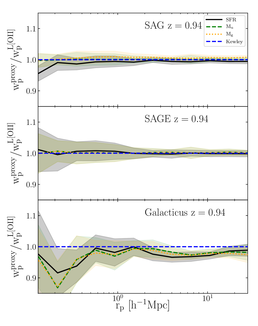
Figure 14: Proxy-to-$L{\left[\mathrm{O\,\textrm{{{ii}}}}\right]}$ ratios of the projected two-point correlation functions of, from top to bottom, sag, sage and galacticus model galaxies at $z\sim 1$. The SAG $L{\left[\mathrm{O\,\textrm{{{ii}}}}\right]}$ is estimated using the get_ emlines code with instantaneous SFR, while sage and galacticus using the average quantity. Galaxies have been selected to have $L{\left[\mathrm{O\,\textrm{{{ii}}}}\right]}$ $>10^{40.4}\,$erg s^-1. The shaded regions represent the effect of the $\sigma_{y}$ scatter in the proxy-$L{\left[\mathrm{O\,\textrm{{{ii}}}}\right]}$ linear relations reported in Table 2. These regions are the $1\sigma$ uncertainties derived from the co-variance of 100 Gaussian realisations with the $L{\left[\mathrm{O\,\textrm{{{ii}}}}\right]}$ proxy considered as mean and $\sigma_{y}$ as scatter. We over plot the Kewley et al. (2004) result as a dashed, blue line.

We further check how the clustering of our model ELGs is sensitive to an $\left[\text{O\,{{ii}}}\right]$ luminosity selection, where $L{\left[\mathrm{O\,\textrm{{{ii}}}}\right]}$ is computed either from the get_ emlines code, or the proxies established above. We consider sag, sage and galacticus model galaxies at $z\sim 1$ and impose on them a minimum luminosity threshold of $L{\left[\mathrm{O\,\textrm{{{ii}}}}\right]}$ $>10^{40.4}\,$erg s^-1.

Fig. 14 shows the ratios between the projected two-point correlation functions obtained from the proxy-to-$L{\left[\mathrm{O\,\textrm{{{ii}}}}\right]}$ relations and those derived from $L{\left[\mathrm{O\,\textrm{{{ii}}}}\right]}$ computed using the get_ emlines code with instantaneous SFR (sag) or average SFR (sage and galacticus). In Fig. 14, we also show the clustering of the data obtained using the conversion from Kewley et al. (2004) given in Eq. 17. For all the models, this clustering is in excellent agreement with the data derived from the get_ emlines $L{\left[\mathrm{O\,\textrm{{{ii}}}}\right]}$ estimation.

For the clustering we adopt the Landy & Szalay (1993) estimator and the two-point function code from Favole et al. (2016b). The shaded regions present the effect of the $\sigma_{y}$ scatter given in Table 2 in the proxy-$L{\left[\mathrm{O\,\textrm{{{ii}}}}\right]}$ linear relations. The dispersion is computed from the covariance of 100 Gaussian realisations with mean the desired proxy and scatter $\sigma_{y}$ (see Section 4.4.1 for further details).

The clustering amplitude remains similar (within 12%) for the different $L{\left[\mathrm{O\,\textrm{{{ii}}}}\right]}$ calculations in all the SAM considered. In particular, in sag and sage galaxies, all the proxies agree within 5% with the get_ emlines and Kewley et al. (2004) results on all scales. On small scales, the SFR proxy in sag declines by 5% and in sage it shows some small fluctuations. In Galacticus, the clustering amplitude diminishes by up to $12\%$ ($4\%$) on small (intermediate) scales when assuming any proxy.

The two point correlation functions at $r_{p}>1h^{-1}$Mpc are consistent with each other, agreeing within the $1\sigma_{y}$ dispersion.

We have investigated further the redshift evolution at $0.6<z<1.2$ and the dependence of different $L{\left[\mathrm{O\,\textrm{{{ii}}}}\right]}$ thresholds of the MultiDark-Galaxies clustering amplitude, both based on estimates from coupling the models with get_ emlines and on the proxies above. In general, we find that increasing both the redshift and the $L{\left[\mathrm{O\,\textrm{{{ii}}}}\right]}$ thresholds, the galaxy number density decreases, resulting in a noiser clustering. Despite this increased noise, we find that model galaxies with $L{\left[\mathrm{O\,\textrm{{{ii}}}}\right]}$ $>10^{41}$erg s^-1 can be more clustered when $L{\left[\mathrm{O\,\textrm{{{ii}}}}\right]}$ is derived from proxies. We find variation among the different proxies used together with one of the three SAMs explored here. This possible dependency with $L{\left[\mathrm{O\,\textrm{{{ii}}}}\right]}$ should be taken into account when using proxies to create fast galaxy catalogues for a particular survey.

Overall, we find that the MultiDark-Galaxies clustering signal is model-dependent. The linear bias is mostly unchanged, however differences are seen at small scales, below 1$h^{-1}$Mpc. The dispersion changes between the different proxies, with the SFR presenting the largest scatter, overall.

Our ELG clustering results show that simple $L{\left[\mathrm{O\,\textrm{{{ii}}}}\right]}$ estimates based on a linear relation with SFR are sufficient for modelling the large scale clustering of $\left[\text{O\,{{ii}}}\right]$ emitters, even if they are not accurate enough to predict the $\left[\text{O\,{{ii}}}\right]$ luminosity function.

4.4.3 [Oii] ELG Halo Occupation Distribution

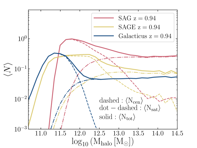
Figure 15: Mean halo occupation distribution of the sag (salmon solid line), sage (yellow solid line) and galacticus (blue solid line) model galaxies with $L{\left[\mathrm{O\,\textrm{{{ii}}}}\right]}$ $>10^{40.4}\,$erg s^-1 at $z\sim 1$. The model $L{\left[\mathrm{O\,\textrm{{{ii}}}}\right]}$ has been computed using get_ emlines with instantaneous SFR for sag galaxies and average SFR for sage and galacticus. The contribution from central galaxies is shown by dashed lines and that for satellites by dot-dashed lines.

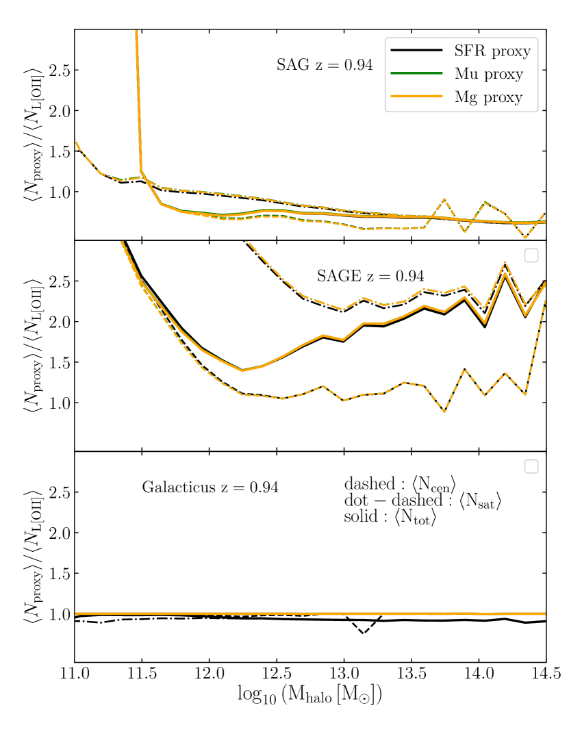
Figure 16: Ratio between the HOD obtained from the $L{\left[\mathrm{O\,\textrm{{{ii}}}}\right]}$ calculated from the proxies indicated in the legend, and $L{\left[\mathrm{O\,\textrm{{{ii}}}}\right]}$ obtained using get_ emlines. From top to bottom, results are shown for the sag, sage and galacticus models.

In Fig. 15, we show the MultiDark-Galaxies mean halo occupation distribution (HOD) for model galaxies selected with $L{\left[\mathrm{O\,\textrm{{{ii}}}}\right]}$ $>10^{40.4}\,$erg s^-1. Here, the model $\left[\text{O\,{{ii}}}\right]$ luminosities have been calculated using the get_ emlines code. We highlight contributions from central and satellite model galaxies. The shapes of the HODs are qualitatively consistent among the different models, with an asymmetric Gaussian for central galaxies, plus maybe a plateau, and a very shallow power law for satellite galaxies. A similar shape has been found using different models for either young or star-forming galaxies, selected in different ways (Zheng et al., 2005; Contreras et al., 2013; Cochrane & Best, 2018; Gonzalez-Perez et al., 2018) and also in measurements derived from observations (Geach et al., 2012; Cochrane et al., 2017; Guo et al., 2018).

The shape of the HOD for central star-forming galaxies is very different from those selected with a cut in either rest-frame optical broad-band magnitudes or stellar mass, which is close to a smooth step function that reaches unity (e.g. Berlind & Weinberg, 2002; Kravtsov et al., 2004). As it can be seen in Fig. 15, the HOD of MultiDark-Galaxies central $\left[\text{O\,{{ii}}}\right]$ emitters does not necessarily reach unity, i.e. it is not guaranteed to find an $\left[\text{O\,{{ii}}}\right]$ emitter in every dark matter halo above a given mass.

We find that the SAG HODs peak at higher halo masses compared to the other two SAMs. The mean halo masses predicted by the sag, sage and galacticus model galaxies are in agreement with the results of Favole et al. (2016a) for BOSS $\left[\text{O\,{{ii}}}\right]$ ELGs at $z\sim 0.8$ and Favole et al. (2017) for SDSS $\left[\text{O\,{{ii}}}\right]$ ELGs at $z\sim 0.1$.

The HOD of MultiDark-Galaxies satellite $\left[\text{O\,{{ii}}}\right]$ emitters is a very shallow power law, closer to a smooth step function. This is similar to what has been inferred for eBOSS $\left[\text{O\,{{ii}}}\right]$ emitters (Guo et al., 2018), but very different to the findings using the galform semi-analytical model (Gonzalez-Perez et al., 2018). This difference is most likely related to a different treatment of gas in this model, as the distribution of satellites in dark matter haloes of different masses is very sensitive to both the modelling of feedback and environmental processes.

In Fig. 16, we display the ratios between the MultiDark-Galaxies HODs selected in $L{\left[\mathrm{O\,\textrm{{{ii}}}}\right]}$, where the luminosity is calculated from either using the get_ emlines code or the proxies indicated in the legend. We find that the differences in the HODs from proxies and get_ emlines are negligible for galacticus and less than $20\%$ for sag at $M_{\rm halo}\,$$\gtrsim 10^{12}{\rm M}_{\odot}$, while sage shows differences above a factor 1.5 in most cases. The $L{\left[\mathrm{O\,\textrm{{{ii}}}}\right]}$ proxies behave very similarly, with negligible differences between them, except for the galacticus SFR proxy, which is slightly lower than the magnitude ones.

In summary, we find different levels of agreement with the get_ emlines results depending on the model considered. However, the HOD remains almost unchanged when different $L{\left[\mathrm{O\,\textrm{{{ii}}}}\right]}$ proxies are assumed.

5 Summary and conclusions

In this work, we have explored how the $\left[\text{O\,{{ii}}}\right]$ luminosity can be estimated for semi-analytic models of galaxy formation and evolution using different methods: (i) by coupling the SAMs with the get_ emlines code (Section 3.1) and (ii) using simple relations between $L{\left[\mathrm{O\,\textrm{{{ii}}}}\right]}$ and global properties such as SFR, broad-band magnitudes and metallicity (Section 4.1).

We have studied the following models from the MultiDark-Galaxies products (Knebe et al., 2018): sag (Cora et al., 2018), sage (Croton et al., 2016) and galacticus (Benson, 2012). All these models are run on the MDPL2 cosmological simulation (Klypin et al., 2016). They were calibrated to a number of observations within $0<z<2$, and they produce SFR and stellar mass functions that evolve similarly to what is observed in this redshift range.

Throughout this study, we have compared our model results with different observational data sets, including DEEP2-FF galaxies with absolute magnitudes (see Section 2.2).

The get_ emlines code to calculate nebular emission lines is publicly available and ideally uses instantaneous SFR as input. However, usually SAMs only output SFRs that are averaged over long time intervals, corresponding to the outputs of the underlying dark matter simulation. From the SAMs under study, only sag provides instantaneous SFRs. We have coupled the get_ emlines code with the sag model using both instantaneous and average SFRs to study the impact that this choice has on the $L{\left[\mathrm{O\,\textrm{{{ii}}}}\right]}$ calculation in post-processing. Assuming as input for the get_ emlines code either the instantaneous or the average SFR, we see a variation below 5% for the dust attenuated $\left[\text{O\,{{ii}}}\right]$ luminosity functions in the range $10^{41}-10^{42.2}\,$erg s^-1, and in the range $10^{41}-10^{3}\,$erg s^-1 for the intrinsic $\left[\text{O\,{{ii}}}\right]$ luminosity functions. These ranges correspond to model ELGs with $1<$SFR (yr^-1M${}_{\odot})<10^{1.5}$. At higher and lower SFRs, there is a larger discrepancy, $<50\%$, in the luminosity functions, when using either the average or the instantaneous SFR. Thus, we find that using average SFRs as inputs for get_ emlines is a good approach when studying average galaxy populations.

The luminosity functions of the MultiDark-Galaxies with $L{\left[\mathrm{O\,\textrm{{{ii}}}}\right]}$ computed using the get_ emlines algorithm are in good agreement with the DEEP2 and VVDS observations over the redshift range $0.6<z<1.2$. The $\left[\text{O\,{{ii}}}\right]$ luminosity, SFR and stellar mass functions of the SAMs all consistently predict a smaller number of massive, star-forming emitters as the redshift increases. The match we find in the $\left[\text{O\,{{ii}}}\right]$ luminosity functions of model and DEEP2 galaxies, where the model $L{\left[\mathrm{O\,\textrm{{{ii}}}}\right]}$ values are computed using the get_ emlines code, cannot guarantee that they are the same identical population of galaxies. In other words, we select the sag, sage and galacticus model galaxies to best reproduce the characteristics of the observed DEEP2 $\left[\text{O\,{{ii}}}\right]$ emitters. These selections return different levels of agreement in the explored parameter spaces, as shown in Figs. 8, 12, 18, 20. A remarkable result from this study is that our model galaxies span the same regions as the observed ones, in all the parameter spaces under study, with overall consistent trends. This suggests that our modelling approach captures the most important physical processes that shape the DEEP2 galaxy sample.

We have also investigated the viability of obtaining $L{\left[\mathrm{O\,\textrm{{{ii}}}}\right]}$ from simple relations with global galactic properties that are usually outputted by galaxy formation models. For this purpose, we use observationally derived relations (Kewley et al., 2004) and linear relations derived for each model. In particular, we explore the $L{\left[\mathrm{O\,\textrm{{{ii}}}}\right]}$ derived using the get_ emlines code as a function of SFR, broad-band magnitudes, age and stellar mass. The SFR, both instantaneous and average, is the physical quantity that, by construction, is most correlated with the $\left[\text{O\,{{ii}}}\right]$ luminosity (with correlation coefficients $r\geq 0.80$ for all the SAMs). Such a tight correlation is well described by a linear scaling law with an associated scatter $\sigma_{\rm{log(SFR)}}$ that varies with $L{\left[\mathrm{O\,\textrm{{{ii}}}}\right]}$ (see Table 2). Other valuable proxies to derive $L{\left[\mathrm{O\,\textrm{{{ii}}}}\right]}$ are the observed-frame $u$ and $g$ broad-band magnitudes, $M_{\rm u}$ and $M_{\rm g}$, which trace the rest-frame UV emission in our redshift range of interest.

We test how feasible it is to use these correlations as proxies for $L{\left[\mathrm{O\,\textrm{{{ii}}}}\right]}$ by studying the evolution of the derived $\left[\text{O\,{{ii}}}\right]$ luminosity functions, mean halo occupation distribution (HOD) and the galaxy clustering signal in $L{\left[\mathrm{O\,\textrm{{{ii}}}}\right]}$ thresholds.

The different methods explored to calculate $L{\left[\mathrm{O\,\textrm{{{ii}}}}\right]}$ result in a range of $\left[\text{O\,{{ii}}}\right]$ luminosity functions. Taking into account the effect of the scatter in the SAG $L{\left[\mathrm{O\,\textrm{{{ii}}}}\right]}$–proxy relations, the luminosity functions from the proxies (including the Kewley et al. (2004) relation from Eq. 17) are in reasonable agreement with the direct get_ emlines estimates. The differences are larger for the relations derived from $M_{g}\,$and SFR in sag at all luminosities, for SFR in sage at $L{\left[\mathrm{O\,\textrm{{{ii}}}}\right]}$ $>10^{42}\,$erg s^-1, and for the magnitude proxies in galacticus. At high luminosities, $L{\left[\mathrm{O\,\textrm{{{ii}}}}\right]}$   derived with most linear proxies result in a lack of bright emitters that increases with luminosity, but remains approximately constant with redshift. The Kewley et al. (2004) relation (Eq. 17) results in a lower number of bright $\left[\text{O\,{{ii}}}\right]$ emitters compared to all the other methods to obtain $L{\left[\mathrm{O\,\textrm{{{ii}}}}\right]}$ in sag and sage, and in a higher number in galacticus.

We find a large variation between the derived $\left[\text{O\,{{ii}}}\right]$ luminosity functions among both the SAMs and the methods used to obtain $L{\left[\mathrm{O\,\textrm{{{ii}}}}\right]}$. Thus, it is important to highlight that, despite the model SFR density evolution being in reasonable agreement with observations, simple relations based on global galaxy properties are not robust estimators for $L{\left[\mathrm{O\,\textrm{{{ii}}}}\right]}$.

We further test the use of simple relations to obtain $L{\left[\mathrm{O\,\textrm{{{ii}}}}\right]}$ for SAMs by measuring the galaxy two-point auto-correlation function for $\left[\text{O\,{{ii}}}\right]$ emitters selected above a given $L{\left[\mathrm{O\,\textrm{{{ii}}}}\right]}$ threshold. We compare the clustering measured from the $\left[\text{O\,{{ii}}}\right]$ proxies with direct predictions from the SAMs coupled with the get_ emlines code and with the Kewley et al. (2004) relationship. The results vary from model to model and the largest fluctuations are seen below $1h^{-1}$Mpc. However, if we account for the effect of the scatter in the proxy-$L{\left[\mathrm{O\,\textrm{{{ii}}}}\right]}$ relation, the discrepancies reconcile with direct luminosity predictions. The large scale bias remains similar for all the models.

By increasing the $L{\left[\mathrm{O\,\textrm{{{ii}}}}\right]}$ threshold, the galaxy number density drops considerably resulting in a noisier clustering signal, which makes the comparison difficult. Despite this increased noise, we find that model galaxies with $L{\left[\mathrm{O\,\textrm{{{ii}}}}\right]}$ $>10^{41}$erg s^-1 can be more clustered when $L{\left[\mathrm{O\,\textrm{{{ii}}}}\right]}$ is derived from proxies (this depends both on the model and the proxy used). This possible dependency with $L{\left[\mathrm{O\,\textrm{{{ii}}}}\right]}$ should be taken into account when using proxies to create fast galaxy catalogues for a particular survey.

There is no direct correspondence between a proxy resulting in a good luminosity function and providing a similar outcome for the clustering.

We also test how the mean HOD of $\left[\text{O\,{{ii}}}\right]$ emitters changes when assuming different proxies compared to the get_ emlines code in the $L{\left[\mathrm{O\,\textrm{{{ii}}}}\right]}$ calculation of our SAMs. We find that the shape of the HOD is consistent with that expected for a star-forming population of galaxies. Quantitatively, the HOD is strongly model-dependent, and we find different levels of agreement between the proxies and the get_ emlines results, in particular at $M_{\rm halo}\,$$\gtrsim 10^{12}{\rm M}_{\odot}$. However, the distributions remain substantially unchanged from one proxy to another for all the models under study.

Our results show that ELGs are different from SFR-selected samples and that the $L{\left[\mathrm{O\,\textrm{{{ii}}}}\right]}$ estimation needs more complex modelling than assuming a linear relation with SFR. Simple $L{\left[\mathrm{O\,\textrm{{{ii}}}}\right]}$ estimates are not accurate enough to predict direct statistics of $L{\left[\mathrm{O\,\textrm{{{ii}}}}\right]}$, as the luminosity function, but they are sufficient for modelling the large scale clustering of $\left[\text{O\,{{ii}}}\right]$ emitters.

New-generation optical and infra-red surveys will provide enormous data sets with unprecedented spectroscopic precision and imaging quality. These observations, together with models of galaxy formation and evolution, will enable us to reach a complete and consistent understanding of both the Universe large scale structure, and the galaxy formation and evolution processes within dark matter haloes. In this context, simple derivations of $L{\left[\mathrm{O\,\textrm{{{ii}}}}\right]}$ might be adequate for the clustering above 1$h^{-1}$Mpc, although at least two simple approximations might be needed to determine the uncertainties.

6 Data availability

The data produced for this article are available at http://popia.ft.uam.es/MultiDarkEmissionLines/ . Here we provide the DEEP2–Firefly observations, both with and without dust attenuation, and the galaxy properties from the sag, sage and galacticus models. For the latter, besides the $\left[\text{O\,{{ii}}}\right]$ emission line, we also include the H$\alpha$, H$\beta$ and $\left[\text{O\,{{iii}}}\right]$ luminosities.

Appendix A SAG model galaxies selected from DEEP2-FF spline

We study the properties of a subset of SAG model galaxies selected to reproduce the $L{\left[\mathrm{O\,\textrm{{{ii}}}}\right]}$ distribution of the DEEP2-FF data approximated by a spline fit in Fig. 4. We compare these model properties with the observational ones from DEEP2-FF.

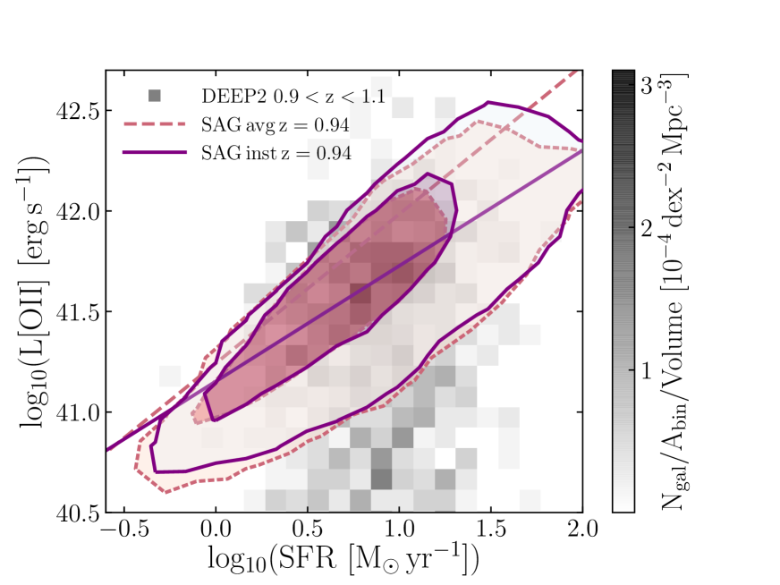
Figure 17: Non-attenuated $\left[\text{O\,{{ii}}}\right]$ luminosity as a function of SFR for the SAG model galaxies at $z\sim 1$ (contours) and the DEEP2-FF observations at $0.9<z<1.1$ (grey, shaded squares). The colour bar represents the observed galaxy number density in each 2D bin normalised by the bin area in units of [dex^-2 Mpc^-3]. Here the SAG model galaxies are selected following the spline fit to the observed DEEP2-FF $L{\left[\mathrm{O\,\textrm{{{ii}}}}\right]}$ distribution shown in Fig. 4. The model $L{\left[\mathrm{O\,\textrm{{{ii}}}}\right]}$ values are calculated by assuming instantaneous (solid, purple contours) and average (dashed, salmon) SFR as input for the get_ emlines prescription. The innermost (outermost) model contours encompass 68% (95%) percent of the galaxy distributions. The diagonal lines represent the $L{\left[\mathrm{O\,\textrm{{{ii}}}}\right]}$-SFR correlations, whose coefficients are reported in Tab. 3.

y=$A$ x+$B$	$A$	$B$	$\sigma_{\rm{y}}$	$r$
y=log10($L{\left[\mathrm{O\,\textrm{{{ii}}}}\right]}$)
x=log10(SFRavg)	0.741$\pm$0.002	41.24$\pm$0.01	0.41	0.92
x=log10(SFRinst)	0.574$\pm$0.003	41.15$\pm$0.01	0.38	0.77
y=$M_{u}\,$
x=log10(SFRavg)	-2.021$\pm$0.006	-18.04$\pm$0.01	1.16	0.88
x=log10(SFRinst)	-2.084$\pm$0.005	-17.88$\pm$0.01	1.17	0.90
y=$M_{g}\,$
x=log10(SFRavg)	-2.006$\pm$0.005	-18.96$\pm$0.01	1.11	0.92
x=log10(SFRinst)	-2.032$\pm$0.005	-18.84$\pm$0.01	1.11	0.93
y=log10(M⋆)
x=log10(SFRavg)	0.859$\pm$0.002	9.15$\pm$0.01	0.47	0.92
x=log10(SFRinst)	0.846$\pm$0.002	9.11$\pm$0.01	0.47	0.90

Table 3: Best-fit parameters of the linear scaling relations found for sag model galaxies at $z=1$ and shown in Fig. 18. The parameter $r$ is the correlation coefficient and $\sigma_{y}$ is the scatter in the $y$-axis. SAG galaxies have been selected in $L{\left[\mathrm{O\,\textrm{{{ii}}}}\right]}$ randomly drawn from the DEEP2-FF spline fit shown in Fig.4.

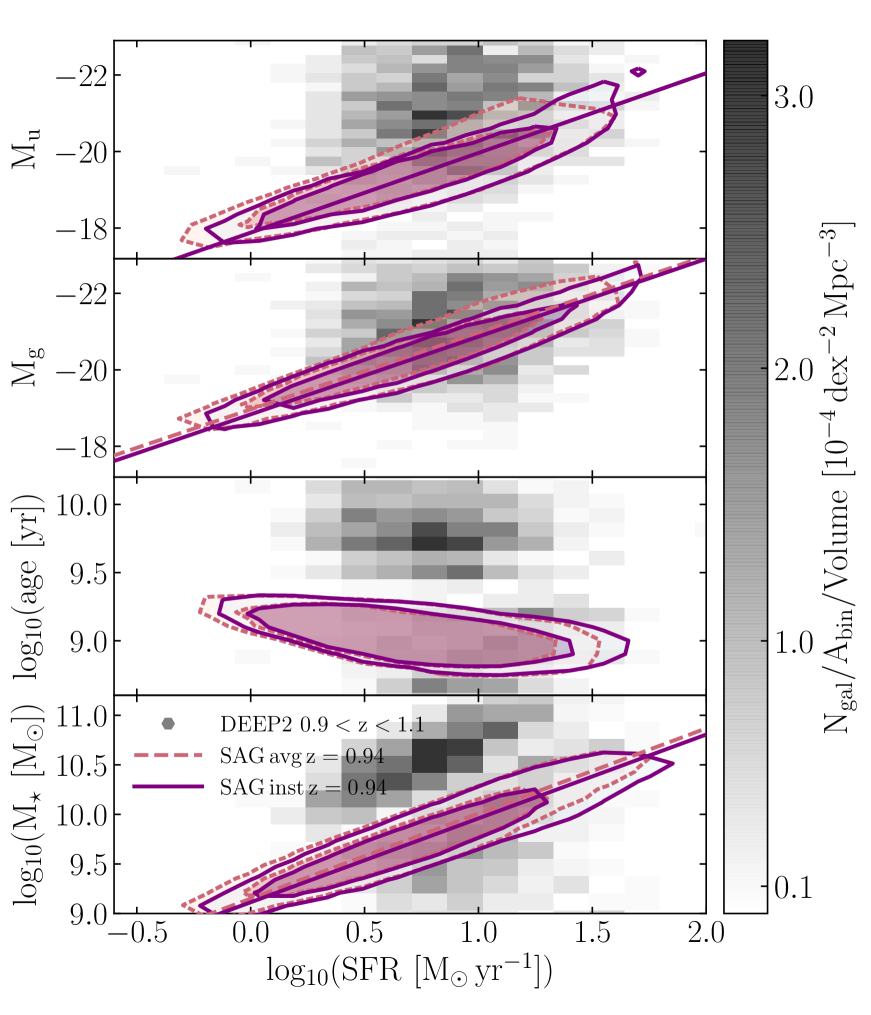
Figure 18: From top to bottom: intrinsic magnitudes, ages and stellar masses as a function of star formation rate for sag model galaxies at $z\sim 1$ (contours) and DEEP2-FF observations at $0.9<z<1.1$ (grey, shaded squares). The model galaxies have been selected following the observed DEEP2-FF distribution approximated by a spline fit, as explained in Sec. 2.2.2. The colour bar shows the number density of DEEP2 galaxies per bin area in units of [dex^-2 Mpc^-3]. The dashed, salmon (solid, purple) contours represent the average (instantaneous) SFRs. The innermost (outermost) contours encompass 68% (95%) of the distributions. The diagonal lines are the linear fits showing the significant correlations, whose coefficients are reported in Table 2, together with the best-fit parameters.

Fig. 17 displays the SAG non-attenuated $\left[\text{O\,{{ii}}}\right]$ luminosities computed from average and instantaneous SFRs as a function of SFR. The bimodality observed in Fig. 5, where the model galaxies are selected by cutting at $\rm{SFR>0}$ and $\rm{log(M_{\star}/M_{\odot})>8.87}$, has now disappeared, but the discrepancy between the two sets of contours is larger, with the instantaneous correlation much shallower than the average one. At SFR$\gtrsim 10^{1}$yr^-1M_⊙, the instantaneous SFR returns higher $L{\left[\mathrm{O\,\textrm{{{ii}}}}\right]}$ values compared to the average SFR. Instead, at SFR$\lesssim 10^{0}$yr^-1M_⊙, the average contours reach fainter luminosities. Compared to the sag results based on simple SFR and stellar mass cuts (see Fig. 5), here both sets of contours span a higher range of $L{\left[\mathrm{O\,\textrm{{{ii}}}}\right]}$ and SFR values. The $L{\left[\mathrm{O\,\textrm{{{ii}}}}\right]}$-SFR correlation based on average (instantaneous) SFR is stronger (less strong) and with a steeper (shallower) slope compared to that for galaxies selected with simple cuts (compare Tabs. 1 and 3), while the scatter is the same.

The DEEP2-FF observations in Fig. 17 seem to span a narrower range in SFR and to go fainter in $L{\left[\mathrm{O\,\textrm{{{ii}}}}\right]}$ compared to the model galaxy contours. However, we highlight that the low-luminosity observational tail has a very low-density of emitters ($\sim 10^{-4}$ in Fig. 17).

In Fig. 18, from top to bottom, we display the intrinsic $u$- and $g$-band absolute magnitudes, the age and stellar mass of the SAG model galaxies selected from the DEEP2-FF spline fit as a function of the average and instantaneous SFRs. Compared to the results based on simple cuts at SFR$\,>0$ yr^-1 M_⊙ and $M_{\star}\,$$>10^{8.87}\,$M_⊙ (see Fig. 8), here the correlations between SFR and magnitudes are steeper and M_u shows a wider scatter in the $y$-axis. On the contrary, the correlation between SFR and stellar mass is shallower for sag galaxies drawn from the DEEP2-FF spline fit and with less scatter in the $y$-axis. The specific values of the correlation parameters and coefficients are reported in Table 3. Overall, sag galaxies selected from the spline fit reach brighter values of $u$- and $g$-band magnitudes compared to their counterparts based on simple SFR and stellar mass cuts (see Fig. 8), which also extend down to fainter magnitudes and smaller stellar masses. As already noticed in Fig. 8, model galaxies have lower ages and stellar masses and they extend into larger SFR values, compared to the DEEP2-FF sample.

Appendix B Evolution of L[Oii] from instantaneous and average SFR

We investigate further the redshift evolution of the small discrepancy generated in $L{\left[\mathrm{O\,\textrm{{{ii}}}}\right]}$ by assuming average instead of instantaneous SFR as input for the get_ emlines code. In Section 3.3, we have studied what happens at $z\sim 1$, now we look over the redshift range $0.6<z<1.2$ to see if there is some evolution.

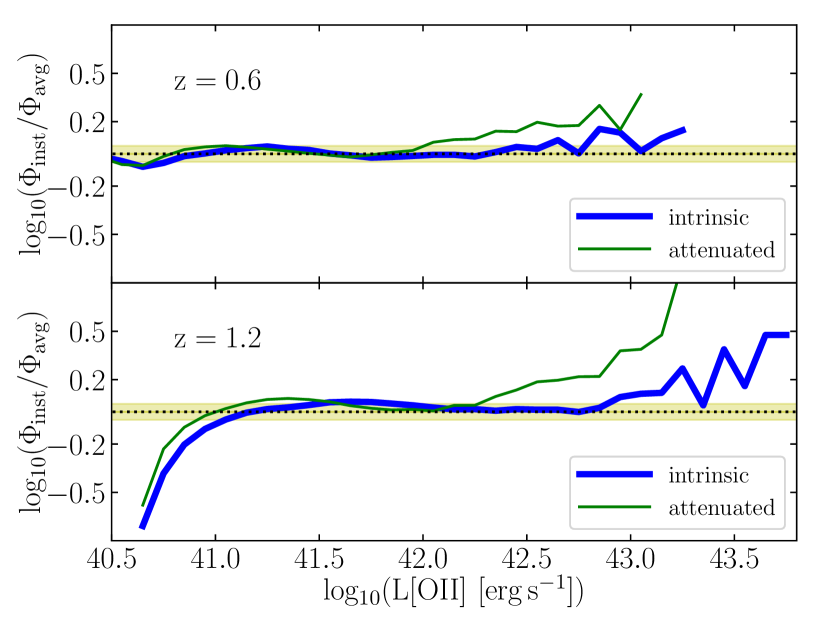
Figure 19: Ratios between the SAG $\left[\text{O\,{{ii}}}\right]$ luminosity functions (thick, blue lines: intrinsic LFs; thin, green: attenuated LFs) at different redshifts computed from average and instantaneous SFR using the method presented in 3.1. The yellow, shaded areas represent the 5% confidence region.

Fig. 19 compares the ratios of the intrinsic (thick, blue lines) and attenuated (thin, green) $\left[\text{O\,{{ii}}}\right]$ luminosity functions obtained from average and instantaneous SFR at different redshifts. We have explored the entire range $0.6<z<1.2$ finding that, as the redshift increases, the instantaneous and average $L{\left[\mathrm{O\,\textrm{{{ii}}}}\right]}$ results tend to agree on a larger luminosity domain. Specifically, the 5% agreement threshold (yellow, shaded region in the plot) is reached for the first time at $z=0.6,1.2$ by galaxies with attenuated $L{\left[\mathrm{O\,\textrm{{{ii}}}}\right]}$ $=10^{41.9},10^{42.3}\,$erg s^-1 and with intrinsic $L{\left[\mathrm{O\,\textrm{{{ii}}}}\right]}$ $=10^{42.6},10^{42.9}\,$erg s^-1, respectively. This result is independent on the presence of attenuation in the $\left[\text{O\,{{ii}}}\right]$ luminosity. At $z\sim 1.2$, we observe a larger discrepancy in both ratios in the faint region due to the larger effect of incompleteness.

Appendix C Global properties of MultiDark-Galaxies

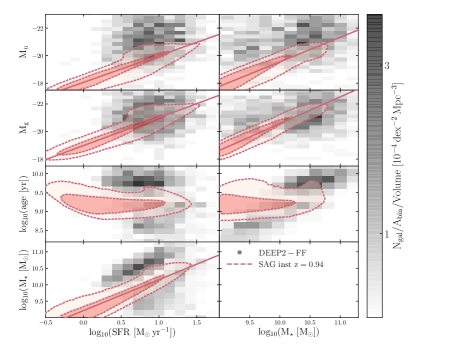
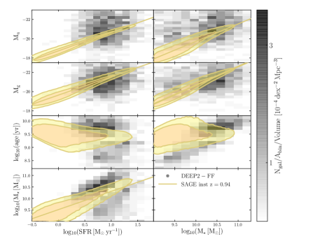
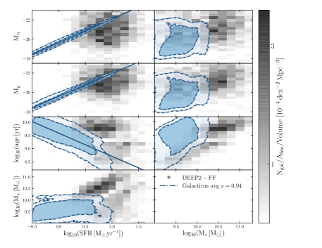
Figure 20: Comparison of pairs of properties for MultiDark-Galaxies at $z=1$ (contours) and DEEP2–FF observations at $0.9<z<1.1$ (grey, shaded squares). The colour bars show the number density of DEEP2 galaxies in each square. From top to bottom, we display sag, sage and galacticus results. A minimum $\left[\text{O\,{{ii}}}\right]$ flux cut of $\rm{5\times 10^{-18}\,\,erg\,s^{-1}\,cm^{-2}}$ has been applied to both data and model galaxies. In each set of panels, from top to bottom, we compare broad-band $u$ and $g$ absolute magnitudes, age and stellar mass as a function of, from left to right, average SFR and stellar mass. The model contours, from inner to outer, represent 68% and 95% of the distributions. The diagonal lines are the linear fits showing the significant correlations, whose coefficients are given in Table 2.

z=1		SAG	SAGE	Galacticus
$M_{u}\,$ =$A$ log10(SFR/(M⊙ yr-1))+$B$	$A$	-1.934$\pm$0.001	-1.941$\pm$0.001	-2.363 $\pm$0.001
	$B$	-18.06$\pm$0.01	-18.74$\pm$0.01	-19.59$\pm$0.01
	$\sigma_{\rm{log(SFR)}}$	0.50	0.53	0.48
	$\sigma_{\rm{M_{u}}}$	1.07	1.05	1.15
	$r$	0.90	0.97	0.99
$M_{g}\,$ =$A$ log10(SFR/(M⊙ yr-1))+$B$	$A$	-2.029$\pm$0.001	-1.916$\pm$0.001	-2.362$\pm$0.001
	$B$	-18.98$\pm$0.01	-19.63$\pm$0.01	-19.59$\pm$0.01
	$\sigma_{\rm{log(SFR)}}$	0.50	0.53	0.48
	$\sigma_{\rm{M_{g}}}$	1.11	1.08	1.15
	$r$	0.91	0.94	0.99
log10(age/yr) = $A$ log10(SFR/(M⊙ yr-1))+$B$	$A$	—	—	-0.869$\pm$0.002
	$B$	—	—	9.58$\pm$0.1
	$\sigma_{\rm{log(SFR)}}$	—	—	0.48
	$\sigma_{\rm{age}}$	—	—	0.54
	$r$	-0.21	-0.34	-0.77
log10(M⋆/M⊙) =$A$ log10(SFR/(M⊙ yr-1))+$B$	$A$	0.939$\pm$0.001	0.794$\pm$0.001	—
	$B$	9.21$\pm$0.01	9.51$\pm$0.01	—
	$\sigma_{\rm{log(SFR)}}$	0.54	0.52	—
	$\sigma_{\rm{log(M\star)}}$	0.50	0.52	—
	$r$	0.87	0.81	0.18
$M_{u}\,$ = $A$ log10(M⋆/M⊙)+$B$	$A$	-1.779$\pm$0.001	-1.820$\pm$0.002	—
	$B$	-1.75$\pm$0.02	-1.52$\pm$0.01	—
	$\sigma_{\rm{log(M\star)}}$	0.54	0.52	—
	$\sigma_{\rm{M_{u}}}$	1.07	1.05	—
	$r$	0.89	0.89	0.15
$M_{g}\,$ = $A$ log10(M⋆/M⊙)+$B$	$A$	-1.941$\pm$0.001	-1.951$\pm$0.001	—
	$B$	-1.17$\pm$0.01	-1.15$\pm$0.02	—
	$\sigma_{\rm{log(M\star)}}$	0.54	1.08	—
	$\sigma_{\rm{M_{g}}}$	1.11	0.52	—
	$r$	0.94	0.94	0.18

Table 4: Best-fit parameters of the linear scaling relations found in MultiDark-Galaxies at $z\sim 1$ and shown in Fig. 20. The parameter $r$ is the correlation coefficient and $\sigma_{y}$ is the scatter in the $y$-axis. The SFR values are instantaneous for sag and average for sage and galacticus. We highlight that we do not quantify the correlation in the DEEP2-FF sample, since this calculation would require accounting for all the observational incompleteness effects, which goes beyond the aim of this work.

We compare pair properties in MultiDark-Galaxies and DEEP2-FF observations to better understand their mutual correlations. We then fit these dependences using linear scaling relations. Fig. 20 displays, from top to bottom, the correlations between broad-band magnitudes, age and stellar mass as a function of SFR and stellar mass of the DEEP2-FF galaxies (grey, shaded squares, colour-coded according to their galaxy number density normalized by the 2D bin area) compared to the MultiDark-Galaxies (contours indicating the 68% and 95% of each distribution). Data and models overlap covering the brighter, more massive and more star-forming region of the parameter space. In particular, the MultiDark-Galaxies only cover the SFR range above the knee shown in Fig. 2.

For such a small observational sample, it is difficult to establish and fit clear correlations among these quantities and between these quantities and $L{\left[\mathrm{O\,\textrm{{{ii}}}}\right]}$ (see also Fig. 12). In order to do this properly, one should account for all the DEEP2-FF incompleteness effects, which goes beyond the scope of our work. Here we show the comparison between the DEEP2-FF emitters and the MultiDark-Galaxies only to verify that our models cover the parameter space of the observational data set.

From the model point of view, we do find clear correlation among most of the physical quantities presented in Fig. 20. Each set of panels shows the results for one model: from top to bottom we display sag, sage and galacticus model galaxies. The relevant correlations ($r\geq 0.6$) are represented as linear fits and the optimal parameters are reported in Table 4, together with their correlation coefficient ($r$) and the associated scatter in the $y$-axis ($\sigma_{\rm{y}}$).

As expected, tight correlation is observed between the star formation rate and the broad-band $u$ and $g$ magnitudes that trace the rest-frame UV emission of a galaxy (see also Section 4.2). Tight correlation is observed also between the magnitudes and the stellar mass in all our model galaxies, except for galacticus. Overall, the DEEP2-FF observations and the MultiDark-Galaxies show a good overlap in the brighter, more star-forming and massive portion of any parameter space. All the model galaxies then extend further down in SFR, stellar mass and magnitudes.

Age does not correlate with SFR neither in the observations, nor in SAG and SAGE mocks. In galacticus, we observe an anti-correlation between age and SFR, meaning that older galaxies are more star-forming, as expected. Age does seem to correlate with stellar mass in DEEP2-FF, however this feature is not reproduced by any of our model galaxies. DEEP2-FF galaxies show a bimodal distribution in age and stellar mass, with an older, less star-forming, very massive population ($age\gtrsim 10^{9.3}\,$yr; $M_{\star}\,$$\gtrsim 10^{10.3}\,$M_⊙) and a younger, more star-forming distribution with less massive galaxies. None of the model galaxies seem to reproduce this bimodality.

sag and sage stellar masses are tightly correlated with their SFRs, but no dependence is observed in galacticus. While the DEEP2-FF quenched population is too sparse to identify any dependence in the stellar mass–SFR plane, the star-forming selection might show some correlation in the higher-mass end of the distribution. However, as already mentioned above, in order to correctly quantify this correlation, we should take into account the incompleteness effects in the data set, but this calculation goes beyond the aim of our analysis. We do not to show the dependence of the above quantities on metallicity since they do not correlate significantly in any of the model galaxies considered.

References

- Alam et al. (2015) Alam S. et al., 2015, \apjs, 219, 12
- Allen et al. (2008) Allen M. G., Groves B. A., Dopita M. A., Sutherland R. S., Kewley L. J., 2008, The Astrophysical Journal Supplement Series, 178, 20
- Allende Prieto et al. (2001) Allende Prieto C., Lambert D. L., Asplund M., 2001, \apjl, 556, L63
- Asplund et al. (2009) Asplund M., Grevesse N., Sauval A. J., Scott P., 2009, \araa, 47, 481
- Baldry et al. (2008) Baldry I. K., Glazebrook K., Driver S. P., 2008, \mnras, 388, 945
- Baldwin et al. (1981) Baldwin J. A., Phillips M. M., Terlevich R., 1981, \pasp, 93, 5
- Baugh (2006) Baugh C. M., 2006, Reports of Progress in Physics, 69, 3101
- Behroozi et al. (2010) Behroozi P. S., Conroy C., Wechsler R. H., 2010, \apj, 717, 379
- Behroozi et al. (2013) Behroozi P. S., Wechsler R. H., Conroy C., 2013, \apj, 770, 57
- Benson (2010) Benson A. J., 2010, \physrep, 495, 33
- Benson (2012) Benson A. J., 2012, \na, 17, 175
- Berlind & Weinberg (2002) Berlind A. A., Weinberg D. H., 2002, \apj, 575, 587
- Boselli et al. (2014) Boselli A., Cortese L., Boquien M., Boissier S., Catinella B., Lagos C., Saintonge A., 2014, \aap, 564, A66
- Bower et al. (2006) Bower R. G., Benson A. J., Malbon R., Helly J. C., Frenk C. S., Baugh C. M., Cole S., Lacey C. G., 2006, \mnras, 370, 645
- Brinchmann et al. (2004) Brinchmann J., Charlot S., Heckman T. M., Kauffmann G., Tremonti C., White S. D. M., 2004, ArXiv, astro-ph/0406220
- Calzetti et al. (2000) Calzetti D., Armus L., Bohlin R. C., Kinney A. L., Koornneef J., Storchi-Bergmann T., 2000, \apj, 533, 682
- Cardelli et al. (1989) Cardelli J. A., Clayton G. C., Mathis J. S., 1989, \apj, 345, 245
- Chabrier (2003) Chabrier G., 2003, \pasp, 115, 763
- Chabrier et al. (2014) Chabrier G., Hennebelle P., Charlot S., 2014, \apj, 796, 75
- Cochrane & Best (2018) Cochrane R. K., Best P. N., 2018, \mnras, 480, 864
- Cochrane et al. (2017) Cochrane R. K., Best P. N., Sobral D., Smail I., Wake D. A., Stott J. P., Geach J. E., 2017, \mnras, 469, 2913
- Collacchioni et al. (2018) Collacchioni F., Cora S. A., Lagos C. D. P., Vega-Martínez C. A., 2018, \mnras, 481, 954
- Comparat et al. (2017) Comparat J. et al., 2017, ArXiv e-prints:1711.06575
- Comparat et al. (2015) Comparat J. et al., 2015, \aap, 575, A40
- Comparat et al. (2016) Comparat J. et al., 2016, \mnras, 461, 1076
- Conroy et al. (2006) Conroy C., Wechsler R. H., Kravtsov A. V., 2006, \apj, 647, 201
- Contreras et al. (2013) Contreras S., Baugh C. M., Norberg P., Padilla N., 2013, \mnras, 432, 2717
- Cooray & Sheth (2002) Cooray A., Sheth R., 2002, \physrep, 372, 1
- Cora (2006) Cora S. A., 2006, \mnras, 368, 1540
- Cora et al. (2018) Cora S. A. et al., 2018, \mnras, 479, 2
- Croton et al. (2006) Croton D. J. et al., 2006, \mnras, 365, 11
- Croton et al. (2016) Croton D. J. et al., 2016, \apjs, 222, 22
- Dawson et al. (2016) Dawson K. S. et al., 2016, \aj, 151, 44
- De Lucia & Blaizot (2007) De Lucia G., Blaizot J., 2007, \mnras, 375, 2
- De Lucia et al. (2010) De Lucia G., Boylan-Kolchin M., Benson A. J., Fontanot F., Monaco P., 2010, \mnras, 406, 1533
- Devriendt et al. (1999) Devriendt J. E. G., Guiderdoni B., Sadat R., 1999, \aap, 350, 381
- Dickey et al. (2016) Dickey C. M. et al., 2016, \apjl, 828, L11
- Draine (2003) Draine B. T., 2003, Annual Review of Astronomy and Astrophysics, 41, 241
- Driver et al. (2018) Driver S. P. et al., 2018, \mnras, 475, 2891
- Eisenstein et al. (2005) Eisenstein D. J. et al., 2005, \apj, 633, 560
- Etherington et al. (2017) Etherington J. et al., 2017, \mnras, 466, 228
- Faber et al. (2003) Faber S. M. et al., 2003, in Society of Photo-Optical Instrumentation Engineers (SPIE) Conference Series, Vol. 4841, Instrument Design and Performance for Optical/Infrared Ground-based Telescopes, Iye M., Moorwood A. F. M., eds., pp. 1657–1669
- Falcón-Barroso & Knapen (2013) Falcón-Barroso J., Knapen J. H., 2013, Secular Evolution of Galaxies
- Favole et al. (2016a) Favole G. et al., 2016a, \mnras, 461, 3421
- Favole et al. (2016b) Favole G., McBride C. K., Eisenstein D. J., Prada F., Swanson M. E., Chuang C.-H., Schneider D. P., 2016b, \mnras, 462, 2218
- Favole et al. (2017) Favole G., Rodríguez-Torres S. A., Comparat J., Prada F., Guo H., Klypin A., Montero-Dorta A. D., 2017, \mnras, 472, 550
- Font et al. (2008) Font A. S., Johnston K. V., Ferguson A. M. N., Bullock J. S., Robertson B. E., Tumlinson J., Guhathakurta P., 2008, \apj, 673, 215
- Gargiulo et al. (2015) Gargiulo I. D. et al., 2015, \mnras, 446, 3820
- Geach et al. (2012) Geach J. E., Sobral D., Hickox R. C., Wake D. A., Smail I., Best P. N., Baugh C. M., Stott J. P., 2012, \mnras, 426, 679
- Gonzalez-Perez et al. (2018) Gonzalez-Perez V. et al., 2018, \mnras, 474, 4024
- Gonzalez-Perez et al. (2014) Gonzalez-Perez V., Lacey C. G., Baugh C. M., Lagos C. D. P., Helly J., Campbell D. J. R., Mitchell P. D., 2014, \mnras, 439, 264
- Groves et al. (2004) Groves B. A., Dopita M. A., Sutherland R. S., 2004, The Astrophysical Journal Supplement Series, 153, 9
- Gruppioni et al. (2015) Gruppioni C. et al., 2015, \mnras, 451, 3419
- Guiderdoni & Rocca-Volmerange (1987) Guiderdoni B., Rocca-Volmerange B., 1987, \aap, 186, 1
- Guo et al. (2018) Guo H. et al., 2018, arXiv:1810.05318 [astro-ph], arXiv: 1810.05318
- Guo et al. (2011) Guo Q. et al., 2011, \mnras, 413, 101
- Hatton et al. (2003) Hatton S., Devriendt J. E. G., Ninin S., Bouchet F. R., Guiderdoni B., Vibert D., 2003, \mnras, 343, 75
- Henriques et al. (2011) Henriques B., Maraston C., Monaco P., Fontanot F., Menci N., De Lucia G., Tonini C., 2011, \mnras, 415, 3571
- Henriques et al. (2015) Henriques B. M. B., White S. D. M., Thomas P. A., Angulo R., Guo Q., Lemson G., Springel V., Overzier R., 2015, \mnras, 451, 2663
- Henriques et al. (2013) Henriques B. M. B., White S. D. M., Thomas P. A., Angulo R. E., Guo Q., Lemson G., Springel V., 2013, \mnras, 431, 3373
- Hirschmann et al. (2017) Hirschmann M., Charlot S., Feltre A., Naab T., Choi E., Ostriker J. P., Somerville R. S., 2017, \mnras, 472, 2468
- Hirschmann et al. (2016) Hirschmann M., De Lucia G., Fontanot F., 2016, \mnras, 461, 1760
- Hirschmann et al. (2012) Hirschmann M., Naab T., Somerville R. S., Burkert A., Oser L., 2012, \mnras, 419, 3200
- Hou et al. (2017) Hou J., Lacey C. G., Frenk C. S., 2017, ArXiv e-prints
- Hunter (2007) Hunter J. D., 2007, Computing In Science & Engineering, 9, 90
- Izquierdo-Villalba et al. (2019) Izquierdo-Villalba D., Bonoli S., Spinoso D., Rosas-Guevara Y., Henriques B. M. B., Hernández-Monteagudo C., 2019, \mnras, 488, 609
- Jiménez et al. (2019) Jiménez E., Contreras S., Padilla N., Zehavi I., Baugh C. M., Gonzalez-Perez V., 2019, arXiv e-prints, arXiv:1906.04298
- Jouvel et al. (2009) Jouvel S. et al., 2009, \aap, 504, 359
- Kauffmann et al. (1993) Kauffmann G., White S. D. M., Guiderdoni B., 1993, \mnras, 264, 201
- Kennicutt (1998) Kennicutt, Jr. R. C., 1998, \araa, 36, 189
- Kewley et al. (2004) Kewley L. J., Geller M. J., Jansen R. A., 2004, \aj, 127, 2002
- Klypin et al. (2016) Klypin A., Yepes G., Gottlöber S., Prada F., Heß S., 2016, \mnras, 457, 4340
- Knebe et al. (2018) Knebe A. et al., 2018, \mnras, 474, 5206
- Kormendy & Ho (2013) Kormendy J., Ho L. C., 2013, \araa, 51, 511
- Kravtsov et al. (2004) Kravtsov A. V., Berlind A. A., Wechsler R. H., Klypin A. A., Gottlöber S., Allgood B., Primack J. R., 2004, \apj, 609, 35
- Kroupa (2001) Kroupa P., 2001, \mnras, 322, 231
- Lagos et al. (2011) Lagos C. D. P., Baugh C. M., Lacey C. G., Benson A. J., Kim H.-S., Power C., 2011, \mnras, 418, 1649
- Lagos et al. (2008) Lagos C. D. P., Cora S. A., Padilla N. D., 2008, \mnras, 388, 587
- Lagos et al. (2013) Lagos C. d. P., Lacey C. G., Baugh C. M., 2013, \mnras, 436, 1787
- Landy & Szalay (1993) Landy S. D., Szalay A. S., 1993, \apj, 412, 64
- Laureijs et al. (2011) Laureijs R. et al., 2011, ArXiv e-prints: 1110.3193
- Levesque et al. (2010) Levesque E. M., Kewley L. J., Graham J. F., Fruchter A. S., 2010, \apj, 712, L26
- Li & White (2009) Li C., White S. D. M., 2009, \mnras, 398, 2177
- Madau & Dickinson (2014) Madau P., Dickinson M., 2014, Annual Review of Astronomy and Astrophysics, 52, 415
- Maraston et al. (2013) Maraston C. et al., 2013, \mnras, 435, 2764
- Maraston & Strömbäck (2011) Maraston C., Strömbäck G., 2011, \mnras, 418, 2785
- Martin et al. (2010) Martin A. M., Papastergis E., Giovanelli R., Haynes M. P., Springob C. M., Stierwalt S., 2010, \apj, 723, 1359
- Matthews et al. (2013) Matthews D. J., Newman J. A., Coil A. L., Cooper M. C., Gwyn S. D. J., 2013, \apjs, 204, 21
- McConnell & Ma (2013) McConnell N. J., Ma C.-P., 2013, \apj, 764, 184
- Merson et al. (2018) Merson A., Wang Y., Benson A., Faisst A., Masters D., Kiessling A., Rhodes J., 2018, \mnras, 474, 177
- Merson et al. (2016) Merson A. I., Baugh C. M., Gonzalez-Perez V., Abdalla F. B., Lagos C. d. P., Mei S., 2016, \mnras, 456, 1681
- Mohammad et al. (2018) Mohammad F. G. et al., 2018, \aap, 610, A59
- Monaco et al. (2014) Monaco P., Benson A. J., De Lucia G., Fontanot F., Borgani S., Boylan-Kolchin M., 2014, \mnras, 441, 2058
- Moustakas et al. (2013) Moustakas J. et al., 2013, \apj, 767, 50
- Moustakas et al. (2006) Moustakas J., Kennicutt, Jr. R. C., Tremonti C. A., 2006, \apj, 642, 775
- Muñoz Arancibia et al. (2015) Muñoz Arancibia A. M., Navarrete F. P., Padilla N. D., Cora S. A., Gawiser E., Kurczynski P., Ruiz A. N., 2015, \mnras, 446, 2291
- Newman et al. (2013) Newman J. A. et al., 2013, \apjs, 208, 5
- Nuza et al. (2013) Nuza S. E. et al., 2013, \mnras, 432, 743
- Orsi et al. (2014) Orsi Á., Padilla N., Groves B., Cora S., Tecce T., Gargiulo I., Ruiz A., 2014, \mnras, 443, 799
- Orsi & Angulo (2018) Orsi Á. A., Angulo R. E., 2018, \mnras, 475, 2530
- Osterbrock (1989) Osterbrock D. E., 1989, Astrophysics of gaseous nebulae and active galactic nuclei
- Pagel et al. (1979) Pagel B. E. J., Edmunds M. G., Blackwell D. E., Chun M. S., Smith G., 1979, \mnras, 189, 95
- Planck Collaboration et al. (2015) Planck Collaboration et al., 2015, ArXiv e-prints
- Prugniel et al. (2007) Prugniel P., Soubiran C., Koleva M., Le Borgne D., 2007, ArXiv, astro-ph/0703658
- Ruiz et al. (2015) Ruiz A. N. et al., 2015, \apj, 801, 139
- Sartoris et al. (2015) Sartoris B. et al., 2015, ArXiv e-prints: 1505.02165
- Schlegel et al. (2015) Schlegel D. J. et al., 2015, in American Astronomical Society Meeting Abstracts, Vol. 225, American Astronomical Society Meeting Abstracts
- Sobral et al. (2012) Sobral D., Best P. N., Matsuda Y., Smail I., Geach J. E., Cirasuolo M., 2012, \mnras, 420, 1926
- Somerville & Davé (2015) Somerville R. S., Davé R., 2015, \araa, 53, 51
- Spitzer (1978) Spitzer L., 1978, Physical processes in the interstellar medium
- Stevens & Brown (2017) Stevens A. R. H., Brown T., 2017, \mnras, 471, 447
- Talia et al. (2015) Talia M. et al., 2015, \aap, 582, A80
- Tomczak et al. (2014) Tomczak A. R. et al., 2014, \apj, 783, 85
- Tonini et al. (2009) Tonini C., Maraston C., Devriendt J., Thomas D., Silk J., 2009, \mnras, 396, L36
- Tremonti et al. (2004) Tremonti C. A. et al., 2004, \apj, 613, 898
- Trujillo-Gomez et al. (2011) Trujillo-Gomez S., Klypin A., Primack J., Romanowsky A. J., 2011, \apj, 742, 16
- Tully & Fisher (1977) Tully R. B., Fisher J. R., 1977, \aap, 54, 661
- Valentino et al. (2017) Valentino F. et al., 2017, \mnras, 472, 4878
- Weinmann et al. (2006) Weinmann S. M., van den Bosch F. C., Yang X., Mo H. J., Croton D. J., Moore B., 2006, \mnras, 372, 1161
- White & Frenk (1991) White S. D. M., Frenk C. S., 1991, \apj, 379, 52
- Wilkinson et al. (2017) Wilkinson D. M., Maraston C., Goddard D., Thomas D., Parikh T., 2017, \mnras, 472, 4297
- Yates (2014) Yates R. M., 2014, The chemical evolution of galaxies in semi-analytic models and observations
- Zheng et al. (2005) Zheng Z. et al., 2005, \apj, 633, 791
- Zheng et al. (2007) Zheng Z., Coil A. L., Zehavi I., 2007, \apj, 667, 760