T-IFISS: a toolbox for adaptive FEM computation

Abstract

T-IFISS is a finite element software package for studying finite element solution algorithms for deterministic and parametric elliptic partial differential equations. The emphasis is on self-adaptive algorithms with rigorous error control using a variety of a posteriori error estimation techniques. The open-source MATLAB framework provides a computational laboratory for experimentation and exploration, enabling users to quickly develop new discretizations and test alternative algorithms. The package is also valuable as a teaching tool for students who want to learn about state-of-the-art finite element methodology.

Key words: finite elements, stochastic Galerkin methods, a posteriori error estimation, adaptive methods, goal-oriented adaptivity, PDEs with random data, parametric PDEs, mathematical software

AMS Subject Classification: 97N80, 65N30, 65N15, 65N50, 35R60, 65C20, 65N22

1 Introduction and software overview

Progress in computational mathematics is frequently motivated and supported by the results of numerical experiments. The well-established IFISS software package [26, 24] is associated with the monograph [25] and is structured as a stand-alone package for studying discretization algorithms for partial differential equations (PDEs) arising in incompressible fluid dynamics. IFISS is also an established starting point for developing code for specialized research applications. The package is currently used in universities around the world to enhance the teaching of advanced courses in mathematics, computational science and engineering. Investigative numerical experiments enable students to develop deduction and interpretation skills and are especially useful in helping students to remember critical ideas in the long term.

The T-IFISS (Triangular IFISS) toolbox extends the IFISS philosophy and design features to finite element approximations on triangular grids for deterministic and stochastic/parametric elliptic partial differential equations. The emphasis of T-IFISS is on self-adaptive algorithms with rigorous error control using a variety of a posteriori error estimation techniques. In the same way as for its precursor, the development of T-IFISS has been motivated by a desire to create a computational laboratory for experimentation and a tool for reproducible research in computational science; indeed, the toolbox enables users not only to quickly explore new discretization strategies and test alternative algorithms, but to replicate, validate and independently verify computational results. Thus, in this article, instead of giving a comprehensive technical description of the software, we aim to highlight and document those features of T-IFISS that are not available in its precursor package IFISS; we will illustrate these features with a series of case studies that demonstrate the efficiency of the software and its utility as a research and teaching tool.

All the test problems that are built into the current version of T-IFISS are associated with steady-state diffusion equations with anisotropic (or uncertain) conductivity coefficients together with mixed (Dirichlet and Neumann) boundary conditions. These PDE problems may be solved on general polygonal domains, including slit domains and domains with holes. It is worth pointing out that many of these (deterministic) test problems could also be solved using general purpose finite element software packages like deal.II [4], DUNE [17], FEniCS [39], and FreeFEM [34]. The attraction of the T-IFISS environment is the ease with which one can test the alternative error estimation, marking, and refinement strategies, develop new strategies, and extend functionality to new problem classes as well as new approximations and solution algorithms. The modular structure of the code allows one to examine interactions between different components in order to achieve favourable convergence properties or minimize the associated computational cost. Finally, the use of the high-level MATLAB syntax ensures readability, accessibility, and quick visualization of the solution, error estimators, and finite element meshes. These features are invaluable in teaching but are not so explicit in other adaptive finite element method (FEM) packages like ALBERTA [51], PLTMG [5], and p1afem [29]. A unique feature of T-IFISS is that it can be used to solve parameter-dependent elliptic PDE problems stemming from uncertainty quantification models. This facility, called stochastic T-IFISS [14], develops the idea of adaptive stochastic Galerkin FEM and provides an effective alternative to traditional sampling methods commonly used for such problems. The only software packages that we know of that have a similar capability are ALEA [23] and SGLib [56].

The following is a brief overview of the functionality available in T-IFISS (including Stochastic T-IFISS) with links to its directory structure (we refer to [50, Appendix B] for more details including the description of the associated data structures):

• computing Galerkin solutions with $P_{1}$ and $P_{2}$ approximations over the specified triangular mesh (directory /diffusion);

• computing stochastic Galerkin FEM solutions with spatial $P_{1}$ and $P_{2}$ approximations over the specified triangular mesh and for the specified polynomial approximation on the parameter domain; the functionality here includes effective iterative solution of very large linear systems stemming from stochastic Galerkin FEM (directory /stoch_diffusion);

• estimating the energy error in the computed Galerkin solution and the error in a quantity of interest derived from this solution (directories /diffusion_error and /goafem, respectively);

• estimating the energy error in the computed stochastic Galerkin solution and the error in a quantity of interest derived from this solution (directories /stoch_diffusion and /stoch_diffusion/stoch_goafem, respectively);

• adaptive refinement of Galerkin approximations, including local adaptive mesh refinement and, in the case of stochastic/parametric problems, adaptive enrichment of multivariable polynomial approximations (directories /diffusion_adaptive and /stoch_diffusion/stoch_diffusion_adapt);

• visualization of Galerkin solutions, goal functionals, error estimators, finite element meshes; plotting convergence history (the error estimates against the number of degrees of freedom) (directory /graphs);

The rest of the article is organized as follows. In the next section, we recall the main ingredients of adaptive FEM and describe their implementation in T-IFISS; we illustrate this with two case studies (solving the diffusion equation with strongly anisotropic coefficient and computing a harmonic function in the L-shaped domain). Section 3 is focused on implementing the goal-oriented error estimation and adaptivity; the case study here demonstrates the capability of the software to approximate the value of a singular solution to the diffusion problem at a fixed point away from the singularity. In section 4, we discuss the implementation of stochastic Galerkin FEM including the associated error estimation and adaptivity. The efficiency of our adaptive algorithm is demonstrated with a representative case study (solving the diffusion equation with parametric coefficient over the L-shaped domain). Some extensions and future developments of the toolbox are briefly outlined in Section 5.

2 Adaptive finite element methods

Adaptive finite element approximations to solutions of partial differential equations are typically computed by iterating the following loop of four component modules:

$$\mathsf{SOLVE}\ \Longrightarrow\ \mathsf{ESTIMATE}\ \Longrightarrow\ \mathsf{MARK}\ \Longrightarrow\ \mathsf{REFINE}.$$ (2.1)

In this section we first describe the implementation of the four components in (2.1) within T-IFISS. This is followed by two case studies that highlight some of the features of the toolbox and demonstrate its utility and its efficiency.

2.1 Main ingredients of adaptive FEM and their implementation in T-IFISS

Module $\mathsf{SOLVE}$. For a given PDE problem, the Galerkin solution defined on a specific (structured or unstructured) triangular mesh is computed by solving the linear system associated with the Galerkin projection of the variational formulation of the problem onto the corresponding finite element space. Two types of ($C^{0}$) finite element approximations are implemented: piecewise linear ($P_{1}$) and piecewise quadratic ($P_{2}$). For either of these approximations, fast computation of the entries in the stiffness matrix and the load vector is achieved by vectorizing the calculations over all the elements. When solving a deterministic problem the resulting linear equation system is solved using the highly optimized sparse direct solver (UMFPACK) that is built into MATLAB and Octave.

Module $\mathsf{ESTIMATE}$. The purpose of this module is two-fold. First, it computes local error indicators that provide information about the distribution of estimated local errors in the computed Galerkin solution; the error indicators may be associated with elements or edges of the underlying triangulation. Second, it computes an estimate of the (total) energy error in the Galerkin solution. This estimate is used to decide whether the stopping tolerance is met. T-IFISS offers a choice of the following three error estimation strategies (EES) for linear ($P_{1}$) approximation.

(EES1) is a local hierarchical error estimator computed via a standard element residual technique (see [1, Section 3.3]) using either piecewise linear or piecewise quadratic bubble functions over subelements obtained by uniform refinements. The local error indicators in this case are computed elementwise by solving $3\times 3$ linear systems (this calculation is vectorized over elements). The total error estimate is calculated as the $\ell_{2}$-norm of the vector of local error indicators.

(EES2) is a global hierarchical estimator (see [6], [1, Section 5]) using piecewise linear bubble functions corresponding to the uniform refinement of the original triangulation. Note that the implementation of this strategy requires solving a sparse linear system associated with a global residual problem. The localizations of the estimator (to either the elements (default option) or the edges of triangulation) gives two types of local error indicators in this EES.

(EES3) is a two-level error estimate employing piecewise linear bubble functions associated with edge midpoints (of the original triangulation); see [44, 43]. In this case, it is natural to choose local error indicators associated with edges (this is the default choice in (EES3)). However, the choice of elementwise error indicators is also offered as an option; these are computed for each interior element from three corresponding edge indicators (or from two indicators for the elements with an edge on the Dirichlet part of the boundary).

There is currently no flexibility with choosing the EES when using quadratic ($P_{2}$) approximation: the local hierarchical error estimation strategy (EES1) is employed with piecewise quartic bubble functions. More specifically, the local error indicators are computed elementwise by solving $9\times 9$ linear systems (again, the calculation is vectorized over elements), and the total error estimate is calculated as the $\ell_{2}$-norm of the vector of local error indicators.

Module $\mathsf{MARK}$. In this module the elements (or edges) with largest error indicators are selected (i.e., marked) for refinement. Two popular marking strategies are currently implemented: the maximum strategy and the Dörfler strategy (also referred to as the equilibration or bulk chasing strategy).

Let $\{\beta(s);\;s\in\mathcal{S}\}$ denote the set of error indicators associated with the elements of the set $\mathcal{S}$ (e.g., $\mathcal{S}$ can be the set of edges or elements of the triangulation). In the maximum marking strategy, that dates back to [3], the element $s\in\mathcal{S}$ is marked if the associated error indicator $\beta(s)$ is larger than a fixed proportion of the maximum among all error indicators. Specifically, for a given marking (or, threshold) parameter $\theta\in[0,1]$, this strategy returns a minimal subset $\mathcal{M}\subseteq\mathcal{S}$ of marked elements such that

$$\beta(s)\geq\theta\max_{s\in\mathcal{S}}\beta(s)\qquad\forall\,s\in\mathcal{M}.$$ (2.2)

Note that in this strategy, smaller values of $\theta$ lead to larger subsets $\mathcal{M}$.

In the Dörfler marking strategy, that was originally introduced in [20], sufficiently many elements are marked such that the combined contribution of the corresponding error indicators is larger than a fixed proportion of the total error estimate. More precisely, given a marking parameter $\theta\in(0,1]$, this strategy builds a subset $\mathcal{M}\subseteq\mathcal{S}$ of minimal cardinality such that $\{\beta(s);\;s\in\mathcal{M}\}$ is the set of $\#\mathcal{M}$ largest error indicators and

$$\sum\limits_{s\in\mathcal{M}}\beta(s)^{2}\geq\theta\sum\limits_{s\in\mathcal{S}}\beta(s)^{2}.$$ (2.3)

Here, smaller values of $\theta$ lead to smaller subsets $\mathcal{M}$.

Figure 1: NVB bisections: (a) one, (b)-(c) two, and (d) three bisections of the edges of the triangular element. Double lines indicate reference edges, black dots indicate the edges to be bisected, and white dots indicate the newest vertices.

Module $\mathsf{REFINE}$. Given the set of marked elements (or, marked edges) that is obtained by employing one of the above marking strategies, local adaptive mesh refinement is performed in T-IFISS by implementing the longest edge bisection (LEB) strategy—a variant of the newest vertex bisection (NVB) method (we refer to [52, 49, 7, 38, 54, 45] for theoretical and implementational aspects of NVB refinements, as well as to [41] for an overview and comparison of NVB with other mesh-refinement techniques). In this method, a reference edge is designated for each triangle $T$ (for the coarsest mesh, this is always the longest edge of $T$), and $T$ is bisected by halving the reference edge; see Figure 1(a). This introduces two new elements, the sons of $T$, for which reference edges are selected. A recursive application of this procedure leads to a conforming mesh, where one, two, or three bisections of the triangle $T$ may be performed; see Figure 1(a)–(d). The refinement by three bisections (see Figure 1(d)) is called the bisec3 refinement. Refining all elements of the given mesh by three bisections results in a (conforming) uniform bisec3 refinement of this mesh.

It is important to emphasize that NVB iteratively refines individual elements by bisecting some (or all) of their edges. Therefore, either the set of marked elements or the set of marked edges can be used as an input to the NVB-based mesh-refinement routine. Furthermore, NVB refinements lead to nested (Lagrange) finite element spaces (see [45, p.179])—an important ingredient in the proof of the contraction property for adaptive finite element approximations, see [45, Section 5] (note that nestedness is not guaranteed for other mesh-refinement techniques, such as red–green or red–green–blue refinements).

As many other modules in the toolbox, the mesh-refinement routine in T-IFISS exploits MATLAB’s vectorization features. More precisely, once the set of marked elements or edges is returned by the module $\mathsf{MARK}$, the mesh-refinement routine identifies the subsets of elements where one, two, or three bisections should be performed (see Figure 1) and then the elements in the three separate subsets are refined simultaneously.

2.2 Numerical case studies

Let us demonstrate the performance of adaptive finite element routines in T-IFISS with two test examples. When doing this, we will illustrate some of the ingredients of adaptive FEM described in the previous subsection.

Example 1.  Let $D=(-1,1)^{2}$ be the square domain. We consider the diffusion equation with a strongly anisotropic coefficient, together with a constant source function and a homogeneous Dirichlet boundary condition:

$$-\nabla\cdot(A\nabla u({\mathbf{x}})) =1,\qquad{\mathbf{x}}=(x_{1},x_{2})\in D,$$ (2.4)

$$u({\mathbf{x}}) =0,\qquad{\mathbf{x}}\in\partial D,$$

where $A=\left[\begin{smallmatrix}1&0\\ 0&100\end{smallmatrix}\right]$. We solve this problem using $P_{1}$ approximation. The solution is depicted in Figure 2(b) and exhibits sharp gradients within the boundary layers along the edges $x_{1}=\pm 1$ of the domain.

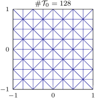
(a)

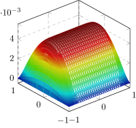
(b)

Figure 2: Example 1: (a) initial coarse mesh; (b) Galerkin solution to problem (2.4).

(a)

(b)

(c)

Figure 3: Example 1: error estimates at each iteration of the adaptive algorithm employing the error estimation strategies (EES1)–(EES3) and using the element-based Dörfler marking with $\theta=0.5$. Here, $N$ denotes the number of degrees of freedom.

In our first experiment for this problem, we ran the adaptive FEM algorithm three times, employing three different error estimation strategies (EES1)–(EES3) with piecewise linear bubble functions as described earlier. In each case, we started with the coarse grid of 128 elements shown in Figure 2(a), fixed the stopping tolerance to tol = 1e-3 and employed the element-based Dörfler marking strategy (2.3) with $\theta=0.5$. The results of computations are presented in Figures 3, 4 and in Table 1.

(a)

(b)

(c)

Figure 4: Example 1: locally refined meshes produced by the adaptive algorithm employing the error estimation strategies (EES1)–(EES3) and using the element-based Dörfler marking with $\theta=0.5$. The header $\#\mathcal{T}_{\ell}$ refers to the number of elements in the mesh at step $\ell$ of the adaptive process.

Figure 3 shows convergence plots for the energy error estimates computed via each of the three strategies. In Figure 4, we plot the locally refined meshes generated by the adaptive algorithm in each of the three cases (for some intermediate tolerance). In Table 1, we have collected the data on iteration counts and mesh refinements for each run of the algorithm. It is evident from these results that using (EES1) leads to unstable reductions in the estimated errors and, as a consequence, to a large number of iterations and an over-refined final mesh. This is because for problem (2.4) with constant coefficients, the elementwise interior residuals for $P_{1}$ approximations have zero contributions to the associated error estimator. In contrast, the adaptive algorithms employing (EES2) and (EES3) lead to essentially monotonic decay of the error estimates; the number of iterations needed to reach the stopping tolerance is nearly the same and similar mesh refinement patterns are generated in both cases. We note that for all three strategies, the error estimates decay with an optimal rate of $\mathcal{O}(N^{-0.5})$, where $N$ is the number of degrees of freedom (d.o.f.).

Adaptive FEM with element-based Dörfler marking ($\theta=0.5$);  tol=1e-3
	(EES1)	(EES2)	(EES3)
$L$	$77$	$25$	$24$
$\eta_{L}$	$9.520$e-$04$	$8.619$e-$04$	$9.668$e-$04$
$\#\mathcal{T}_{L}$	57,347	36,390	30,498
${\color[rgb]{0,0,0}n_{L}}$	28,296	17,875	14,934

Table 1: Example 1: output when solving (2.4) using alternative error estimation strategies; $L$ denotes the total number of iterations, $\eta_{L}$, $\#\mathcal{T}_{L}$, and ${\color[rgb]{0,0,0}n_{L}}$ refer to the final error estimate, the number of elements in the final mesh, and the number of degrees of freedom at the final iteration, respectively.

In our second experiment, we ran the adaptive algorithm driven by two-level error estimates (i.e., using (EES3)) and employed the edge-based Dörfler marking (2.3) with $\theta=0.5$ (we use the same tolerance and the same coarse grid as before). In this experiment, for the error estimate at each iteration of the adaptive algorithm, we calculated the effectivity index (i.e., the ratio between the error estimate and a surrogate approximation of the true error, computed by running the adaptive algorithm with $P_{2}$ approximation with a tighter tolerance of tol = 2e-5). In Figure 5(a), we plot the energy error estimates at each iteration. Comparing this plot with the one in Figure 3(c), we can see improvements in terms of the monotonicity of the error decay and in terms of the number of iterations. The computed effectivity indices for each iteration of the algorithm are plotted in Figure 5(b).

(a)

(b)

Figure 5: Example 1: (a) error estimates at each iteration of the adaptive algorithm employing (EES3) and the edge-based Dörfler marking with $\theta=0.5$, (b) the associated effectivity indices.

In our third experiment, we repeated the previous adaptive procedure with two smaller stopping tolerances. The overall computational times together with the contributions for each of the components in (2.1) are reported in Table 2.

Adaptive FEM with edge-based Dörfler marking ($\theta=0.5$)
	tol=1e-3	tol=5e-4	tol=1e-4
$L$	$16$	$19$	$27$
$\eta_{L}$	$9.661$e-$04$	$4.923$e-$04$	$8.168$e-$05$
${\color[rgb]{0,0,0}n_{L}}$	16,261	63,864	2,181,895
$t$ (SOLVE)	$0.167$	$0.811$	$49.567$
$t$ (ESTIMATE)	$0.324$	$2.013$	$107.107$
$t$ (MARK)	$0.004$	$0.016$	$0.656$
$t$ (REFINE)	$0.101$	$0.366$	$15.394$
$t$ (overall)	$3.090$	$7.937$	$439.862$

Table 2: Example 1: the outputs of running the adaptive algorithm employing the error estimation strategy (EES3) for three different tolerances. Here, $L$, $\eta_{L}$, and $n_{L}$ are as in Table 1. All times $t$ are in seconds and the timings for individual modules are recorded at the final adaptive step.

Example 2.  This experiment addresses the question posed by Nick Trefethen and Abi Gopal to the readers of the NA Digest in November 2018 (see [55, 33]). The community was challenged to compute (to a high accuracy) the point-value close to singularity for a harmonic function in the L-shaped domain. More precisely, let $D=(-1,1)^{2}\setminus(-1,0]^{2}$ and consider the following problem:

$$-{\color[rgb]{0,0,0}\nabla^{2}}u({\mathbf{x}}) =0,\qquad {\mathbf{x}}=(x_{1},x_{2})\in D,$$ (2.5)

$$u({\mathbf{x}}) =(1-x_{1})^{2},\qquad {\mathbf{x}}\in\partial D.$$

The goal is to compute $u(0.01,0.01)$ to at least 8-digit accuracy (the exact value is $1.02679192610\ldots$; see [33]).

In this example, we set the stopping tolerance tol = 4e-5 and ran the adaptive FEM algorithm with $P_{2}$ approximation together with element-based Dörfler marking with $\theta=0.5$. The prescribed tolerance was satisfied after 38 iterations (final number of d.o.f. was 253,231, run time 59.6 sec), giving the value $u(0.01,0.01)\approx 1.02679192311$, which is accurate to 9 digits. Figure 6 depicts the finite element solution to problem (2.5) and shows the convergence plot for the estimated energy errors (together with the optimal rate) as well as the mesh refinement pattern, plotted here for an intermediate tolerance.

(a)

(b)

(c)

Figure 6: Example 2: (a) Galerkin solution to problem (2.5); (b) error estimates at each iteration of the adaptive algorithm with $P_{2}$ approximations and tol = 4e-5; (c) adaptively refined mesh generated by the algorithm for an intermediate tolerance of 1e-3.

3 Goal-oriented adaptivity

The error estimation strategies described in the previous section provide a mechanism for controlling approximation errors in the (global) energy norm. However, in many practical applications, simulations often target a specific quantity of interest (typically, a local feature of the solution) called the goal functional. In such cases, the energy norm of the error is likely to be of limited interest. The implementation of goal-oriented error estimation and adaptivity in T-IFISS is the focus of this section. We also discuss a representative case study to show the efficiency of the adopted approach.

3.1 Goal-oriented error estimation in the abstract setting

We start by describing a general idea of the goal-oriented error estimation strategy implemented in T-IFISS. Let $V$ be a Hilbert space and denote by $V^{\prime}$ its dual space. Let $B:V\times V\to{\mathbb{R}}$ be a continuous, elliptic, and symmetric bilinear form with the associated energy norm $|\|\,\cdot\,\||$, i.e., $|\|\,v\,\||^{2}:=B(v,v)$ for all $v\in V$. Given two continuous linear functionals $F,G\in V^{\prime}$, our aim is to approximate $G(u)$, where $u\in V$ is the unique solution of the primal problem:

$$B(u,v)=F(v)\quad\text{for all $v\in V.$}$$ (3.1)

To this end, the standard approach (see, e.g., [27, 48, 9, 32]) considers $z\in V$ as a unique solution to the dual problem:

$$B(v,z)=G(v)\quad\text{for all $v\in V$.}$$ (3.2)

Let $V_{h}$ be a finite dimensional subspace of $V$. Let $u_{h}\in V_{h}$ (resp., $z_{h}\in V_{h}$) be a unique Galerkin approximation of the solution to the primal (resp., dual) problem, i.e.,

$$B(u_{h},v_{h})=F(v_{h})\quad(\text{resp., }B(v_{h},z_{h})=G(v_{h}))\qquad\text{for all $v_{h}\in V_{h}.$}$$

Then, it follows that

$$\lvert G(u)-G(u_{h})\rvert=\lvert B(u-u_{h},z)\rvert=\lvert B(u-u_{h},z-z_{h})\rvert\leq|\|\,u-u_{h}\,\||\,|\|\,z-z_{h}\,\||,$$ (3.3)

where the second equality holds due to Galerkin orthogonality.

Assume that $\mu=\mu(u_{h})$ and $\zeta=\zeta(z_{h})$ are reliable estimates for the energy errors $|\|\,u-u_{h}\,\||$ and $|\|\,z-z_{h}\,\||$, respectively, i.e.,

$$|\|\,u-u_{h}\,\||\lesssim\mu\quad\text{and}\quad|\|\,z-z_{h}\,\||\lesssim\zeta$$

(here, $a\lesssim b$ means the existence of a generic positive constant $C$ such that $a\leq Cb$). Hence, inequality (3.3) implies that the product $\mu\,\zeta$ is a reliable error estimate for the approximation error in the goal functional:

$$\lvert G(u)-G(u_{h})\rvert\lesssim\mu\,\zeta.$$ (3.4)

3.2 Marking in goal-oriented adaptivity

Having computed two Galerkin solutions $u_{h}$, $z_{h}$, the corresponding energy error estimates $\mu(u_{h})$, $\zeta(z_{h})$, and the reliable estimate $\mu(u_{h})\,\zeta(z_{h})$ of the error in the goal functional (see (3.4)), a goal-oriented adaptive FEM (GOAFEM) algorithm proceeds by executing the $\mathsf{MARK}$ and $\mathsf{REFINE}$ modules of the standard adaptive loop (2.1).

While the module $\mathsf{REFINE}$ simply performs local mesh refinement as explained in the previous section, the marking procedure in the GOAFEM algorithm requires special care. Specifically, since the error in the goal functional is controlled by the product of the energy error estimates for two Galerkin approximations (the primal and dual ones), the edge-marking for bisection (or, the element-marking for refinement) must take into account the local error indicators associated with both approximations. Thus, given the set of local error indicators associated with the primal (resp., dual) Galerkin solution $u_{h}$ (resp., $z_{h}$), let $\mathcal{M}^{u}$ (resp., $\mathcal{M}^{z}$) denote the set of element edges that would be marked for bisection in order to enhance this Galerkin solution (to that end, one can use, e.g., the Dörfler marking strategy, see (2.3)). There exist several strategies for combining the two sets $\mathcal{M}^{u}$ and $\mathcal{M}^{z}$ into a single marking set $\mathcal{M}$ that is used for mesh refinement in the goal-oriented adaptive algorithm. Four different strategies are implemented in T-IFISS:

(GO–MARK1) following [35], the marking set $\mathcal{M}$ is simply the union of $\mathcal{M}^{u}$ and $\mathcal{M}^{z}$;

(GO–MARK2) following [42], the marking set $\mathcal{M}$ is defined as the set of minimal cardinality between $\mathcal{M}^{u}$ and $\mathcal{M}^{z}$;

(GO–MARK3) following [8], the set $\mathcal{M}$ is obtained by performing Dörfler marking on the set of combined error indicators $\beta(E)$ associated with edges of the triangulation, where

$$\beta(E):=\big{(}\mu^{2}_{E}\,\zeta^{2}+\zeta^{2}_{E}\,\mu^{2}\big{)}^{1/2}$$

and $\mu_{E}$ (resp., $\zeta_{E}$) is the local contribution to $\mu$ (resp., $\zeta$) associated with the edge $E$;

(GO–MARK4) this marking strategy is a modification of (GO–MARK2); following [28], we compare the cardinality of ${\mathcal{M}}^{u}$ and that of ${\mathcal{M}}^{z}$ to define

$${\mathcal{M}}_{\star}:={\mathcal{M}}^{u}\quad\hbox{and}\quad{\mathcal{M}}^{\star}:={\mathcal{M}}^{z}\qquad \hbox{if $\#{\mathcal{M}}^{u}\leq\#{\mathcal{M}}^{z}$},$$

$${\mathcal{M}}_{\star}:={\mathcal{M}}^{z}\quad\hbox{and}\quad{\mathcal{M}}^{\star}:={\mathcal{M}}^{u}\qquad \hbox{otherwise};$$

the marking set ${\mathcal{M}}$ is then defined as the union of ${\mathcal{M}}_{\star}$ and those $\#{\mathcal{M}}_{\star}$ edges of ${\mathcal{M}}^{\star}$ that have the largest error indicators.

Comparing these four strategies, it is proved in [28, Theorem 13] that the GOAFEM algorithm employing marking strategies (GO–MARK2)–(GO–MARK4) generates approximations that converge with optimal algebraic rates, whereas only suboptimal convergence rates have been proved for marking strategy (GO–MARK1); cf. [28, Remark 4] and [35, Section 4]. The numerical results in [28] suggest that (GO–MARK4) is more effective than the original strategy (GO–MARK2) in terms of the overall computational cost. Our own experience is that (GO–MARK4) is a competitive strategy in every example that has been tested. Consequently, we have made it the default option within the code.

3.3 Numerical case study

In order to demonstrate the effectiveness of the goal-oriented adaptive strategy described in the previous subsection, let us consider the following test example.

Example 3.  Let us consider the model problem given by (2.4) with $A=\text{Id}$ on a slit domain $D_{\delta}=(-1,1)^{2}\setminus\overline{T}_{\delta}$, where $T_{\delta}=\text{conv}\{(0,0),(-1,\delta),(-1,-\delta)\}$ with $\delta=0.005$. It is known that solution $u$ to the (primal) problem in this example exhibits a singularity induced by the slit in the domain (see Figure 7(b)). Our aim, however, is to demonstrate the capability of the software to approximate the value of $u$ at some fixed point ${\mathbf{x}}_{0}\in D$ away from the slit (in the experiments below, we set ${\mathbf{x}}_{0}=(0.4,-0.5)$). In order to define the corresponding bounded goal functional $G$, it is common to fix a sufficiently small $r>0$ and first introduce the mollifier $g_{0}$ as follows (cf. [48]):

$$g_{0}({\mathbf{x}})=g_{0}({\mathbf{x}};{\mathbf{x}}_{0},r):=\begin{cases}C\exp\left(-\frac{r^{2}}{r^{2}-|{\mathbf{x}}-{\mathbf{x}}_{0}|^{2}}\right)&\text{if $|{\mathbf{x}}-{\mathbf{x}}_{0}|<r$},\\ 0&\text{otherwise.}\end{cases}$$ (3.5)

Here, the constant $C$ is chosen such that $\int_{D}g_{0}({\mathbf{x}})\,\mathrm{d}{\mathbf{x}}=1$ (for sufficiently small $r$ such that $\text{supp}(g_{0}({\mathbf{x}};{\mathbf{x}}_{0},r))\subset D$, one has $C\approx 2.1436\,r^{-2}$; see, e.g., [48]). Then, the functional $G$ in (3.2) reads as

$$G(v)=\int_{D}g_{0}({\mathbf{x}})v({\mathbf{x}})\,\mathrm{d}{\mathbf{x}}\quad\text{for all }v\in H^{1}_{0}(D).$$

Note that if $u({\mathbf{x}})$ is continuous in a neighborhood of ${\mathbf{x}}_{0}$, then $G(u)$ converges to the point value $u({\mathbf{x}}_{0})$ as $r$ tends to zero.

(a)

(b)

Figure 7: Example 3: (a) initial coarse mesh in the GOAFEM algorithm; (b) the primal Galerkin solution.

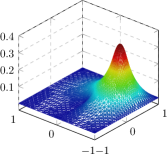
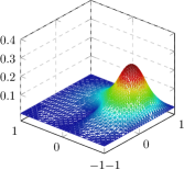
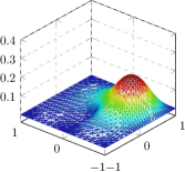
Figure 8: Example 3: adaptively refined triangulations (top row) and the dual Galerkin solutions (bottom row) computed using the mollifier $g_{0}$ in (3.5) with $r=0.2,\,0.35,\,0.5$.

We started with the coarse triangulation depicted in Figure 7(a) in all the experiments. In the first experiment, we fixed the stopping tolerance to be tol = 3e-4 and ran the GOAFEM algorithm to compute dual Galerkin solutions for different values of the radius $r$ in (3.5). For the $\mathsf{SOLVE}$ step, we used $P_{1}$ approximations for both primal and dual solutions. Within the $\mathsf{ESTIMATE}$ module, the energy errors in both solutions were estimated using the two-level error estimation strategy (EES3) described earlier. Given the error indicators for primal and dual solutions, the algorithm employed the edge-based Dörfler marking (2.3) with $\theta=0.3$ in combination with the strategy (GO–MARK4) above. Figure 8 shows the refined triangulations (top row) and the corresponding dual Galerkin solutions (bottom row) for $r=0.2,\,0.35,\,0.5$. We note that the triangulations generated by the algorithm adapt to the features of both primal and dual solutions: the triangulations are refined in the vicinity of each corner (with particularly strong refinement near the tip of the slit) and in a neighborhood of ${\mathbf{x}}_{0}$ (with stronger refinement for smaller values of $r$).

Focusing now on the case $r=0.2$, we set tol = 8e-5 in the second experiment and ran the GOAFEM algorithm without changing the settings. The results we obtained are shown in Figure 9. In Figure 9(a), we plot the energy error estimates for primal and dual Galerkin approximations, the estimates of the error in the goal functional, as well as the reference errors in the goal functional (i.e., $|G(u_{\rm ref})-G(u_{h})|$) at each iteration of the GOAFEM algorithm. Here, the reference Galerkin solution $u_{\rm ref}$ is computed using the triangulation obtained by two uniform refinements of the final triangulation generated by the GOAFEM algorithm. We observe that all error estimates as well as the reference error in the goal functional converge with optimal rates. The effectivity indices for the goal-oriented error estimation at each iteration of the algorithm are plotted in Figure 9(b). This plot shows that the product of energy error estimates for the primal and dual Galerkin solutions provides a reasonably accurate estimate for the error in approximating the goal functional $G(u)$.

(a)

(b)

Figure 9: Example 3: (a) error estimates at each iteration of the GOAFEM algorithm employing the marking strategy (GO–MARK4); (b) the associated effectivity indices.

4 Adaptive FEM for parametric PDEs

In this section, we address the design of components of the adaptive algorithm when working in a parametric PDE setting. Before discussing the details of our implementation, we formulate the model problem with parametric input data and briefly describe the idea of stochastic Galerkin FEM (SGFEM). Readers interested in theoretical aspects of SGFEM are referred to [31], [19] and [2].

4.1 Stochastic Galerkin FEM

Let $D\subset{\mathbb{R}}^{2}$ be a Lipschitz domain (called the physical domain) with polygonal boundary $\partial D$ and let $\Gamma:=\prod_{m=1}^{\infty}[-1,1]$ denote the infinitely-dimensional hypercube (called the parameter domain). We consider the elliptic boundary value problem

$$-\nabla\cdot(a\nabla u) =f\quad \text{in }D\times\Gamma,$$ (4.1)

$$u =0\quad \text{on }\partial D\times\Gamma,$$

where the scalar coefficient $a$ (and, hence, the solution $u$) depends on a countably infinite number of scalar parameters, i.e., $a=a({\mathbf{x}},{\mathbf{y}})$ and $u=u({\mathbf{x}},{\mathbf{y}})$ with ${\mathbf{x}}\in D$, ${\mathbf{y}}\in\Gamma$, and the differentiation in $\nabla$ is with respect to ${\mathbf{x}}=(x_{1},x_{2})$. We assume that $f=f({\mathbf{x}})\in H^{-1}(D)$ and that the parametric coefficient $a$ has affine dependence on the parameters, i.e.,

$$a({\mathbf{x}},{\mathbf{y}})=a_{0}({\mathbf{x}})+\sum_{m=1}^{\infty}y_{m}a_{m}({\mathbf{x}})\quad\text{for }{\mathbf{x}}\in D\text{ and }{\mathbf{y}}=(y_{m})_{m\in{\mathbb{N}}}\in\Gamma,$$ (4.2)

where the scalar functions $a_{m}\in W^{1,\infty}(D)$ ($m\in{\mathbb{N}}_{0}$) satisfy the following inequalities:

$$0<a_{0}^{\min}\leq a_{0}({\mathbf{x}})\leq a_{0}^{\max}<\infty\quad\text{for almost all }{\mathbf{x}}\in D$$ (4.3)

and

$$\tau:=\frac{1}{a_{0}^{\rm min}}\,\sum_{m=1}^{\infty}\|a_{m}\|_{L^{\infty}(D)}<1.$$ (4.4)

The weak formulation of (4.1) is posed in the framework of the Bochner space $V:=L^{2}_{\pi}(\Gamma;H^{1}_{0}(D))$. Here, $\pi\,{=}\,\pi({\mathbf{y}})$ is a probability measure on $(\Gamma,\mathcal{B}(\Gamma))$ with $\mathcal{B}(\Gamma)$ being the Borel $\sigma$-algebra on $\Gamma$, and we assume that $\pi({\mathbf{y}})$ is the product of symmetric Borel probability measures $\pi_{m}$ on $[-1,1]$, i.e., $\pi({\mathbf{y}})=\prod_{m=1}^{\infty}\pi_{m}(y_{m})$. For a given $f\in H^{-1}(D)$, the weak solution $u\in V$ satisfies

$$B(u,v)=F(v):=\int_{\Gamma}\int_{D}f({\mathbf{x}})v({\mathbf{x}},{\mathbf{y}})\,\mathrm{d}{\mathbf{x}}\,\mathrm{d}\pi({\mathbf{y}})\quad\text{for all }v\in V.$$ (4.5)

Here,

$$B(u,v) :=B_{0}(u,v)+\sum_{m=1}^{\infty}\int_{\Gamma}\int_{D}y_{m}a_{m}({\mathbf{x}})\nabla u({\mathbf{x}},{\mathbf{y}})\cdot\nabla v({\mathbf{x}},{\mathbf{y}})\,\mathrm{d}{\mathbf{x}}\,\mathrm{d}\pi({\mathbf{y}}),$$

$$B_{0}(u,v) :=\int_{\Gamma}\int_{D}a_{0}({\mathbf{x}})\nabla u({\mathbf{x}},{\mathbf{y}})\cdot\nabla v({\mathbf{x}},{\mathbf{y}})\,\mathrm{d}{\mathbf{x}}\,\mathrm{d}\pi({\mathbf{y}}).$$ (4.6)

The following three coefficient expansions (CEs) of the type (4.2) are implemented in Stochastic T-IFISS.

(CE1) Let $D=(-1,1)^{2}$ and suppose that the coefficient $a=a({\mathbf{x}},{\mathbf{y}})$ in (4.1) is a parametric representation of a second-order random field with prescribed mean $\mathbb{E}[a]$ and covariance function $\text{Cov}[a]$. Assume that $\text{Cov}[a]$ is the separable exponential covariance function given by

$$\text{Cov}[a]({\mathbf{x}},{\mathbf{x}}^{\prime})=\sigma^{2}\exp\left(-\frac{|x_{1}-x_{1}^{\prime}|}{l_{1}}-\frac{|x_{2}-x_{2}^{\prime}|}{l_{2}}\right),$$

where ${\mathbf{x}},\,{\mathbf{x}}^{\prime}\in D$, $\sigma$ denotes the standard deviation, and $l_{1},l_{2}$ are correlation lengths. In this case, $a({\mathbf{x}},{\mathbf{y}})$ can be written in the form (4.2) using the Karhunen–Loève-type expansion [40] such that

$$a_{0}({\mathbf{x}}):=\mathbb{E}[a]({\mathbf{x}}),\quad a_{m}({\mathbf{x}}):=c\,\sqrt{\lambda_{m}}\,\varphi_{m}({\mathbf{x}}),\quad m\in{\mathbb{N}},$$

where $\{(\lambda_{m},\varphi_{m})\}_{m=1}^{\infty}$ are the eigenpairs of the operator $\int_{D}\text{Cov}[a]({\mathbf{x}},{\mathbf{x}}^{\prime})\varphi({\mathbf{x}}^{\prime})\mathrm{d}{\mathbf{x}}^{\prime}$, and the constant $c>0$ is chosen such that ${\rm Var}(c\,y_{m})=1$ for all $m\in{\mathbb{N}}$. Note that analytical expressions for $\lambda_{m}$ and $\varphi_{m}$ for the square domain $D$ follow from the corresponding formulas derived in [31, pp. 28–29] for the one-dimensional case.

(CE2) Following [21, Section 11.1], we set $a_{0}({\mathbf{x}}):=1$, ${\mathbf{x}}\in D$, and choose the coefficients $a_{m}({\mathbf{x}})$ in (4.2) to represent planar Fourier modes of increasing total order:

$$a_{m}({\mathbf{x}}):=\alpha_{m}\cos(2\pi\beta_{1}(m)\,x_{1})\cos(2\pi\beta_{2}(m)\,x_{2})\quad\text{for all $m\in{\mathbb{N}}$},$$ (4.7)

where $\alpha_{m}:=Am^{-\tilde{\sigma}}$ are the amplitudes of the coefficients, $\tilde{\sigma}>1$, the constant $A$ is chosen such that $\tau=A\zeta(\tilde{\sigma})=0.9$ (here, $\zeta$ denotes the Riemann zeta function), and $\beta_{1}$, $\beta_{2}$ are defined as

$$\beta_{1}(m):=m-k(m)(k(m)+1)/2\ \ \hbox{and}\ \ \beta_{2}(m):=k(m)-\beta_{1}(m),$$

with $k(m):=\lfloor-1/2+\sqrt{1/4+2m}\rfloor$ for all $m\in{\mathbb{N}}$. The following two values of the decay parameter $\tilde{\sigma}$ are used in test problems: $\tilde{\sigma}=2$ (slow decay) and $\tilde{\sigma}=4$ (fast decay).

(CE3) Finally, we consider the following parametric coefficient (cf. [40, Example 9.37]):

$$a({\mathbf{x}},\tilde{\mathbf{y}})=1+c\,\sum_{i=0}^{\infty}\sum_{j=0}^{\infty}\sqrt{\lambda_{ij}}\varphi_{ij}({\mathbf{x}})y_{ij},\quad\tilde{\mathbf{y}}=(y_{ij})_{i,j\in{\mathbb{N}}_{0}},$$ (4.8)

where $\lambda_{ij}=\bar{\lambda}_{i}\,\bar{\lambda}_{j}$, $\varphi_{ij}({\mathbf{x}})=\bar{\varphi}_{i}(x_{1})\,\bar{\varphi}_{j}(x_{2})$, $y_{ij}\in[-1,1]$ ($i,j\in{\mathbb{N}}_{0}$) with $\bar{\lambda}_{0}:=1/2$, $\bar{\varphi}_{0}(t):=1$, $\bar{\lambda}_{k}:=\frac{1}{2}\exp(-\pi k^{2}\ell^{2})$, $\bar{\varphi}_{k}(t):=\sqrt{2}\cos(\pi kt)$ ($k\in{\mathbb{N}})$, and the constant $c>0$ is chosen such that ${\rm Var}(c\,y_{i,j})=1$ for all $i,j\in{\mathbb{N}}_{0}$.

As shown in [40, Example 9.37], the parametric representation (4.8) stems from the Karhunen-Loève expansion of a random field with the mean $\mathbb{E}[a]=1$ and covariance function close to the isotropic covariance $c(\textbf{x})=(4\ell^{2})^{-1}\,\exp(-\pi(x_{1}^{2}+x_{2}^{2})/(4\ell^{2}))$, where $\ell$ is the correlation length. For our implementation, we set $\ell=1$ and reorder the terms in the double sum in (4.8) to write the coefficient $a({\mathbf{x}},\tilde{\mathbf{y}})$ in the form (4.2) with

$$a_{0}({\mathbf{x}}):=1,\quad a_{m}({\mathbf{x}}):=c\,\sqrt{\lambda_{m}}\,\varphi_{m}({\mathbf{x}}),\quad y_{m}\in[-1,1],\quad m\in{\mathbb{N}},$$

where $\lambda_{1}\geq\lambda_{2}\geq\ldots$.

In each coefficient expansion (CE1)–(CE3), parameters $y_{m}$ ($m\in{\mathbb{N}}$) are the images of independent mean-zero random variables on $\Gamma_{m}=[-1,1]$. The following two types of bounded random variables (RVs) are implemented in Stochastic T-IFISS.

(RV1) Uniformly distributed random variables. In this case, $\mathrm{d}\pi_{m}=\mathrm{d}y_{m}/2$ and the orthonormal polynomial basis in $L^{2}_{\pi_{m}}(\Gamma_{m})$ is comprised of scaled Legendre polynomials.

(RV2) Truncated Gaussian random variables. In this case, $\mathrm{d}\pi_{m}=p(y_{m})\mathrm{d}y_{m}$ with

$$p(y_{m})=\frac{\exp(-y_{m}^{2}/(2\sigma_{0}^{2}))}{\sigma_{0}\sqrt{2\pi}(2\Phi(1/\sigma_{0})-1)},\quad m\in{\mathbb{N}},$$ (4.9)

where $\Phi(\cdot)$ is the Gaussian cumulative distribution function and $\sigma_{0}$ is a parameter measuring the standard deviation. The corresponding orthonormal polynomial basis in $L^{2}_{\pi_{m}}(\Gamma_{m})$ is formed by the so-called Rys polynomials; see, e.g., [30, Example 1.11].

A key observation that motivates the stochastic Galerkin FEM is that the Bochner space $V=L^{2}_{\pi}(\Gamma;H^{1}_{0}(D))$ is isometrically isomorphic to $H^{1}_{0}(D)\otimes L^{2}_{\pi}(\Gamma)$. Mimicking this tensor-product construction, the finite-dimensional subspace $V_{\mathbb{X}\mathbb{P}}\subset V$ is defined as $V_{\mathbb{X}\mathbb{P}}:=\mathbb{X}\otimes\mathbb{P}$; here, $\mathbb{X}=\mathbb{X}_{h}$ is a finite element space associated with a conforming triangulation $\mathcal{T}_{h}$ of $D$ and $\mathbb{P}=\mathbb{P}_{\mathscr{P}}$ is a polynomial space on $\Gamma$ associated with a finite index set $\mathscr{P}$. Specifically,

$$\mathbb{X}=\mathbb{X}_{h}:=\text{span}\{\phi_{i};\;i=1,\ldots N_{\mathbb{X}}\}\subset H^{1}_{0}(D),\quad N_{\mathbb{X}}:=\dim(\mathbb{X})$$ (4.10)

and

$$\mathbb{P}=\mathbb{P}_{\mathscr{P}}:=\text{span}\Big{\{}\mathsf{P}_{\nu}({\mathbf{y}})=\prod_{m\in{\mathbb{N}}}\mathsf{P}_{\nu_{m}}^{m}(y_{m});\;\nu\in\mathscr{P}\Big{\}}\subset L^{2}_{\pi}(\Gamma)\ \ \text{with $\mathscr{P}\subset\mathscr{I}$},$$

where $\{\mathsf{P}_{n}^{m}:n\in{\mathbb{N}}_{0}\}$ is an orthonormal basis of $L^{2}_{\pi_{m}}(-1,1)$ and $\mathscr{I}$ denotes the countable set of finitely supported multi-indices, i.e.,

$$\mathscr{I}:=\big{\{}\nu=(\nu_{m})_{m\in{\mathbb{N}}};\;\nu_{m}\in{\mathbb{N}}_{0}\text{ for all }m\in{\mathbb{N}},\ \#\text{supp}(\nu)<\infty\big{\}}$$

with $\text{supp}(\nu):=\{m\in{\mathbb{N}};\;\nu_{m}\neq 0\}$.

The Galerkin discretization of (4.5) reads as follows: find $u_{\mathbb{X}\mathbb{P}}\in V_{\mathbb{X}\mathbb{P}}$ such that

$$B(u_{\mathbb{X}\mathbb{P}},v)=F(v)\quad\text{for all }v\in V_{\mathbb{X}\mathbb{P}}.$$ (4.11)

Note that $\dim(V_{\mathbb{X}\mathbb{P}})=\dim(\mathbb{X}_{h}){\color[rgb]{0,0,0}\times}\dim(\mathbb{P}_{\mathscr{P}})$. Therefore, if a large number of random variables is used to represent the input data, then computing high-fidelity stochastic Galerkin approximations with standard polynomial subspaces on $\Gamma$ (e.g., the spaces of tensor-product or complete polynomials) becomes prohibitively expensive. This motivates the development of adaptive SGFEM algorithms that incrementally refine spatial ($\mathbb{X}$-) and parametric ($\mathbb{P}$-) components of Galerkin approximations by iterating the standard adaptive loop (2.1). The implementation details are discussed in the following subsections.

4.2 Module $\mathsf{SOLVE}$. Linear algebra aspects of SGFEM

Recalling the definitions of $\mathbb{X}_{h}$ and $\mathbb{P}_{\mathscr{P}}$, the Galerkin solution $u_{\mathbb{X}\mathbb{P}}$ is sought in the form

$$u_{\mathbb{X}\mathbb{P}}=\sum_{i=1}^{N_{\mathbb{X}}}\sum_{j=1}^{N_{\mathbb{P}}}u_{ij}\phi_{i}({\mathbf{x}})\mathsf{P}_{\kappa(j)}({\mathbf{y}}),$$ (4.12)

where $N_{\mathbb{P}}:=\dim(\mathbb{P})=\#\mathscr{P}$, $\kappa$ is a bijection $\{1,2,\ldots,N_{\mathbb{P}}\}\to\mathscr{P}$, and the coefficients $u_{ij}$ are computed by solving the linear system $A{\mathbf{u}}={\mathbf{b}}$ with block structure. Specifically, the solution vector ${\mathbf{u}}$ and the right-hand side vector ${\mathbf{b}}$ are given by

$${\mathbf{u}}=[{\mathbf{u}}_{1}\ {\mathbf{u}}_{2}\ \ldots\ {\mathbf{u}}_{N_{\mathbb{P}}}]^{T}\text{ \ and \ }{\mathbf{b}}=[{\mathbf{b}}_{1}\ {\mathbf{b}}_{2}\ \ldots\ {\mathbf{b}}_{N_{\mathbb{P}}}]^{T},$$

respectively, with

$${\mathbf{u}}_{j}:=[u_{1j}\;u_{2j}\;\ldots\;u_{N_{\mathbb{X}}j}]^{T},\quad j=1,\ldots,N_{\mathbb{P}},$$

$$[{\mathbf{b}}_{t}]_{s}:=\langle 1,\mathsf{P}_{\kappa(t)}\rangle_{\pi}\,\int_{D}f({\mathbf{x}})\phi_{s}({\mathbf{x}})\,\mathrm{d}{\mathbf{x}},\quad s=1,\ldots,N_{\mathbb{X}},\ \ t=1,\ldots,N_{\mathbb{P}};$$

the coefficient matrix $A$ is given by (see, e.g., [40, Section 9.5])

$$A=G_{0}\otimes K_{0}+\sum_{m=1}^{M_{\mathscr{P}}}G_{m}\otimes K_{m},$$ (4.13)

where $M_{\mathscr{P}}$ is the number of active parameters in the index set $\mathscr{P}$,

$$[G_{0}]_{tj}:=\langle\mathsf{P}_{\kappa(j)},\mathsf{P}_{\kappa(t)}\rangle_{\pi}=\delta_{tj},\quad[G_{m}]_{tj}:=\langle y_{m}\mathsf{P}_{\kappa(j)},\mathsf{P}_{\kappa(t)}\rangle_{\pi}\ \ (m=1,\ldots,M_{\mathscr{P}})$$

with $t,j=1,\ldots,N_{\mathbb{P}}$, and $K_{m}$ are the finite element (stiffness) matrices defined by

$$[K_{m}]_{si}:=\int_{D}a_{m}\nabla\phi_{i}\cdot\nabla\phi_{s}\,\mathrm{d}{\mathbf{x}},\quad m=0,1,\ldots,M_{\mathscr{P}},\ \ s,i=1,\ldots,N_{\mathbb{X}}.$$

The design of an efficient linear solver is a crucial ingredient of the stochastic Galerkin approximation process. Rather than computing a (memory intensive) sparse factorization of the coefficient matrix, a matrix-free iterative solver is needed. The key idea is that the matrix-vector products with $A$ can be computed from its sparse matrix components by exploiting the Kronecker product structure, without assembling $A$ itself. The iterative solver that enables this process within T-IFISS is a bespoke implementation of the Minimum Residual algorithm, called EST_MINRES [53]. The MINRES algorithm is designed to solve symmetric (possibly indefinite) linear equation systems and requires the action of $A$ on a given vector at every iteration, see [25, Section 2.4]. Using this strategy the storage overhead (in addition to the component matrices $K_{0},\ldots,K_{M_{\mathscr{P}}},G_{1},\ldots,G_{M_{\mathscr{P}}}$) is for five vectors of length $N_{\mathbb{P}}\cdot N_{\mathbb{X}}$.

A crucial ingredient in the design of a fast iterative solver is preconditioning. The standard choice of preconditioning operator in this context is the parameter-free matrix operator

$$P=G_{0}\otimes K_{0}=I\otimes K_{0}.$$

The action of $P^{-1}{\mathbf{r}}$, where ${\mathbf{r}}$ is the current residual vector, is needed at every iteration—this can be done efficiently by computing a single sparse triangular factorization of the matrix $K_{0}$ and then performing $N_{\mathbb{P}}$ forward and backward substitutions on the components of the residual vector. Theoretical analysis of the preconditioned operator given in [47] shows that the eigenvalues of the preconditioned operator are bounded away from zero and bounded away from infinity independently of the discretization parameters $N_{\mathbb{X}}$ and $N_{\mathbb{P}}$. This means that the number of preconditioned EST_MINRES iterations needed to satisfy a fixed residual reduction tolerance will not grow unboundedly when the discretization parameters are changed. In practice, the number of iterations needed to satisfy the default tolerance of 1e-10 is less than 20, independent of the finite element mesh resolution and the number of active indices.

4.3 Module $\mathsf{ESTIMATE}$. Error estimation in SGFEM

Stochastic Galerkin approximations are built from two distinct discretizations: the spatial (finite element) discretization over the physical domain $D$ and the parametric (polynomial) approximation on the parameter domain $\Gamma$. Therefore, there are two distinct sources of discretization error arising from the choice of the finite element space $\mathbb{X}$ and the polynomial space $\mathbb{P}$. This fact determines the structure of a posteriori estimates for the energy errors in SGFEM approximations as combinations of spatial and parametric contributions (cf. [21, 22, 10, 15]).

The spatial errors in SGFEM approximations are estimated by extending the strategies (EES1)–(EES3) described in §2 to tensor-product discretizations. For example, in (EES1), each local (elementwise) error estimator, denoted by $e_{\mathbb{X}}|_{K}$ ($K\in\mathcal{T}_{h}$), now lives in the tensor-product space $\mathbb{Y}|_{K}\otimes\mathbb{P}_{\mathscr{P}}$, where $\mathbb{Y}|_{K}$ is the local space of piecewise linear or piecewise quadratic bubble functions. These error estimators are computed by solving local residual problems of the following type (see [10, Section 6.2] for details):

$$B_{0,K}(e_{\mathbb{X}}|_{K},v)=\text{Res}_{K}(a,f,u_{\mathbb{X}\mathbb{P}};v)\quad\forall\,v\in\mathbb{Y}|_{K}\otimes\mathbb{P}_{\mathscr{P}},$$ (4.14)

where $B_{0,K}$ is the elementwise bilinear form associated with the parameter-free term $a_{0}$ in the coefficient expansion (cf. (4.6)). This construction of the error estimator enables fast linear algebra for solving (4.14). Indeed, the coefficient matrix in the linear system associated with (4.14) has a very simple structure: it is the Kronecker product of a $3\times 3$ reduced stiffness matrix and the identity matrix of dimension $N_{\mathbb{P}}=\dim(\mathbb{P})$. As a result, the action of the inverse of this coefficient matrix can be effected by a block $LDL^{T}$ factorization of the element stiffness matrices followed by a sequence of $N_{\mathbb{P}}$ backward and forward substitutions. Furthermore, since the factorizations and triangular solves are logically independent, the entire computation is vectorized over the finite elements that define the spatial subdivision. We refer to [12, Section 3] for details of the global hierarchical (EES2) and the two-level (EES3) error estimation strategies in the context of the SGFEM.

The parametric errors in SGFEM approximations are estimated using the hierarchical approach in the spirit of [6]. To that end, we first introduce the finite index set $\mathscr{Q}_{\mathscr{P}}$ as a “neighborhood” of the index set $\mathscr{P}$. More precisely, for a fixed $\overline{M}\in{\mathbb{N}}$, we define

$$\mathscr{Q}_{\mathscr{P}}:=\big{\{}\nu\in\mathscr{I}\setminus\mathscr{P};\;\nu=\mu\pm\varepsilon^{(m)}\text{ for some }\mu\in\mathscr{P}\text{ and some }m=1,\dots,M_{\mathscr{P}}+\overline{M}\big{\}},$$ (4.15)

where $\varepsilon^{(m)}:=(\varepsilon^{(m)}_{1},\varepsilon^{(m)}_{2},\dots)$ ($m\in{\mathbb{N}}$) denotes the Kronecker delta index such that $\varepsilon^{(m)}_{k}=\delta_{mk}$ for all $k\in{\mathbb{N}}$, and $M_{\mathscr{P}}\in{\mathbb{N}}$ is the number of active parameters in $\mathscr{P}$.

For a given $\mathscr{P}\subset\mathscr{I}$, the index set $\mathscr{Q}_{\mathscr{P}}$ contains only those “neighbors” of all indices in $\mathscr{P}$ that have up to $M_{\mathscr{P}}+\overline{M}$ active parameters, that is $\overline{M}$ parameters more than currently activated in the index set $\mathscr{P}$ (we refer to [15, Section 4.2] for theoretical underpinnings of this construction). Then, the parametric error estimator $e_{\mathbb{P}}$ is computed as a combination of the contributing estimators $e_{\mathbb{P}}^{(\nu)}$ associated with individual indices $\nu\in\mathscr{Q}_{\mathscr{P}}$, i.e., $e_{\mathbb{P}}=\sum_{\nu\in\mathscr{Q}_{\mathscr{P}}}e_{\mathbb{P}}^{(\nu)}$, where each contributing estimator $e_{\mathbb{P}}^{(\nu)}\in\mathbb{X}\otimes\text{span}(\mathsf{P}_{\nu})$, $\nu\in\mathscr{Q}_{\mathscr{P}}$, is computed by solving the linear system associated with the following discrete formulation:

$$B_{0}(e_{\mathbb{P}}^{(\nu)},v\mathsf{P}_{\nu})=F(v\mathsf{P}_{\nu})-B(u_{\mathbb{X}\mathbb{P}},v\mathsf{P}_{\nu})\quad\text{for all $v\in\mathbb{X}$}.$$ (4.16)

Note that the coefficient matrix of this linear system represents the assembled stiffness matrix corresponding to the parameter-free term $a_{0}$ in (4.2), and is therefore the same for all $\nu\in\mathscr{Q}_{\mathscr{P}}$. Once the stiffness matrix has been factorized, the estimators $e_{\mathbb{P}}^{(\nu)}$ are computed independently by using forward and backward substitutions.

Once the spatial and parametric error estimators have been computed, the total error estimate $\eta$ is calculated via

$$\eta:=\Big{(}\|e_{\mathbb{X}}\|^{2}_{0}+\|e_{\mathbb{P}}\|^{2}_{0}\Big{)}^{1/2}=\bigg{(}\sum\limits_{K\in\mathcal{T}_{h}}\big{\|}e_{\mathbb{X}}|_{K}\|^{2}_{0,K}+\sum\limits_{\nu\in\mathscr{Q}_{\mathscr{P}}}\big{\|}e_{\mathbb{P}}^{(\nu)}\big{\|}^{2}_{0}\bigg{)}^{1/2},$$ (4.17)

where $\|\cdot\|_{0}$ (resp., $\|\cdot\|_{0,K}$) denotes the norm induced by the bilinear form $B_{0}$ (resp., $B_{0,K}$).

4.4 Marking and refinement in adaptive SGFEM

The module $\mathsf{ESTIMATE}$ supplies local spatial error indicators associated with elements or edges of triangulation (e.g., $e_{\mathbb{X}}|_{K}$ for the error estimation strategy (EES1)) as well as the contributing parametric error indicators $e_{\mathbb{P}}^{(\nu)}$ associated with individual indices $\nu\in\mathscr{Q}_{\mathscr{P}}$. In the module $\mathsf{MARK}$, the largest error indicators are selected independently for spatial and for parametric components of Galerkin approximations. To that end, one of the marking strategies described in §2 (i.e., either the maximum or the Dörfler strategy) is employed. In Stochastic T-IFISS, the same marking strategy is used for both spatial and parametric components with marking thresholds $\theta_{\mathbb{X}}$ and $\theta_{\mathbb{P}}$, respectively. However, a simple modification of the code will allow one to use different marking strategies for different components of Galerkin approximations.

Thus, at each iteration of the adaptive SGFEM algorithm, the output of the module $\mathsf{MARK}$ contains two sets: the set of marked elements in the current mesh $\mathcal{T}_{h}$ to be refined (or, the set of edges to be bisected) and the set $\mathscr{M}\subseteq\mathscr{Q}_{\mathscr{P}}$ of marked indices to be added to the current index set $\mathscr{P}$ (note that choosing $\overline{M}>1$ in (4.15) allows one to activate more than one new parameter at the next iteration of the adaptive loop). The finite-dimensional space $V_{\mathbb{X}\mathbb{P}}$ is then enhanced within the module $\mathsf{REFINE}$ by performing either spatial refinement (as described in  §2) or parametric refinement (simply by adding $\mathscr{M}$ to $\mathscr{P}$). The question then arises which type of refinement (spatial or parametric) should be performed at a given iteration.

A traditional strategy for choosing between the two refinements is based on the dominant error estimator contributing to the total error estimate $\eta$ defined in (4.17); cf. [21, 22, 15]. This strategy is referred to as version 1 of the adaptive algorithm implemented in Stochastic T-IFISS. An alternative strategy is referred to as version 2 of the implemented algorithm: here, the refinement type that leads to a larger estimated error reduction is chosen at each iteration; see [13, 11]. This strategy exploits the fact that local spatial error indicators (e.g., $\|e_{\mathbb{X}}|_{K}\|_{0,K}$ ($K\in\mathcal{T}_{h}$) in the error estimation strategy (EES1)) and individual parametric error indicators $\|e_{\mathbb{P}}^{(\nu)}\|_{0}$ ($\nu\in\mathscr{Q}_{\mathscr{P}}$) provide effective estimates of the error reduction that would be achieved by performing, respectively, a local refinement of the current mesh (e.g., by refining the element $K$) and a selective enrichment of the parametric component of the current Galerkin approximation (by adding the index $\nu\in\mathscr{Q}_{\mathscr{P}}$ to the current index set $\mathscr{P}$). We refer to [10, Theorem 5.1] and [11, Corollary 3] for the underpinning theoretical results and to [13] and [11, Section 5] for comprehensive numerical studies of the two versions of the adaptive algorithm and different marking strategies.

4.5 Numerical case study

We conclude this section with a representative case study that demonstrates the efficiency of our adaptive SGFEM algorithm.

Example 4. We consider the parametric model problem (4.1) on the L-shaped domain $D=(-1,1)^{2}\setminus(-1,0]^{2}$. We set $f({\mathbf{x}})=(1-x_{1})^{-0.4}$ and choose the parametric coefficient $a({\mathbf{x}},{\mathbf{y}})$ in the form (4.2), where $a_{0}$ and $a_{m}$ ($m\in{\mathbb{N}}$) are as specified by the coefficient expansion (CE2) with $\tilde{\sigma}=2$ and $y_{m}$ ($m\in{\mathbb{N}}$) are the images of independent truncated Gaussian random variables with zero mean on $\Gamma_{m}=[-1,1]$ (see (RV2), where we set $\sigma_{0}=1$). The mean and the variance of an SGFEM solution to this problem are shown in Figure 10(a)–(b), whereas Figure 10(c) depicts a typical locally refined mesh generated by the adaptive SGFEM algorithm. Note how the adaptively refined mesh effectively identifies the areas of singular behavior of the mean field—in the vicinity of the reentrant corner (due to a geometric singularity) and in the vicinity of the edge $x_{1}=1$ (due to a singular right-hand side function).

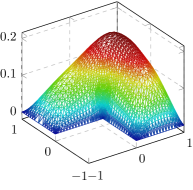
(a)

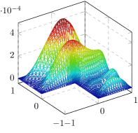
(b)

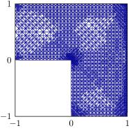
(c)

Figure 10: Example 4: (a)–(b) mean and variance of the SGFEM solution; (c) a typical locally refined mesh generated by the adaptive SGFEM algorithm.

When running the adaptive SGFEM algorithm, we start with a uniform mesh consisting of 96 right-angled triangles and an initial index set $\mathscr{P}_{0}:=\{(0,0,0,\ldots,),\;(1,0,0,\ldots,)\}$. For the error estimation module, we employ the two-level spatial error estimator (EES3) combined with the hierarchical parametric error estimators associated with individual indices $\nu\in\mathscr{Q}_{\mathscr{P}}$ (see (4.16) and (4.15), where we set $\overline{M}:=1$). We use Dörfler marking for spatial and parametric components of Galerkin approximations (for the spatial component, we mark the edges of the mesh).

Figure 11: Example 4: error estimates at each iteration of the adaptive SGFEM algorithm for different sets of marking parameters.

In our first experiment we ran the adaptive SGFEM algorithm (in version 2) with the following four sets of Dörfler marking parameters (with different stopping tolerances):
(i) $\theta_{\mathbb{X}}=1$, $\theta_{\mathbb{P}}=1$ (no adaptivity in either of the components), tol=5.1e-3;
(ii) $\theta_{\mathbb{X}}=0.7$, $\theta_{\mathbb{P}}=1$ (adaptive refinement only for spatial component), tol=4e-3;
(iii) $\theta_{\mathbb{X}}=1$, $\theta_{\mathbb{P}}=0.7$ (adaptive refinement only for parametric component), tol=4e-3 ;
(iv) $\theta_{\mathbb{X}}=0.7$, $\theta_{\mathbb{P}}=0.9$ (adaptive refinement of both components), tol=3e-3.
For each run of the algorithm, the error estimates computed at each iteration are plotted in Figure 11. The error estimates can be seen to decrease at every iteration. However, in cases (i)–(iii), the decay rate either eventually deteriorates (cases (i) and (ii)), due to the number of degrees of freedom growing very fast, or it is significantly slower (case (iii)) than in the case of adaptivity being used for both components of SGFEM approximations (case (iv)). This shows that, for the same level of accuracy, adaptive refinement of both components results in more balanced approximations with fewer degrees of freedom and leads to the fastest convergence rate for the parameter choices in this experiment.

Iteration		Evolution of the index set
0		(0 0 0 0 0 0)
		(1 0 0 0 0 0)
7		(0 1 0 0 0 0)
		(2 0 0 0 0 0)
11		(0 0 1 0 0 0)
		(1 1 0 0 0 0)
		(3 0 0 0 0 0)
14		(0 0 0 1 0 0)
		(1 0 1 0 0 0)
		(2 1 0 0 0 0)
		(0 2 0 0 0 0)
16		(0 0 0 0 1 0)
		(2 0 1 0 0 0)
		(1 0 0 1 0 0)
		(4 0 0 0 0 0)
18		(0 0 0 0 0 1)
		(1 0 0 0 1 0)
		(3 1 0 0 0 0)
		(0 1 1 0 0 0)
		(1 2 0 0 0 0)
		(2 0 0 1 0 0)
		(3 0 1 0 0 0)
		(1 0 0 0 0 1)

Table 3: Example 4: evolution of the index set when running adaptive SGFEM algorithm with $\theta_{\mathbb{X}}=0.7$ and $\theta_{\mathbb{P}}=0.9$.

To give an indication of the algorithmic efficiency, we provide further details of the run in case (iv). In this computation, which took 927 seconds, the stopping tolerance 3e-3 was met after 19 iterations. The final triangulation generated by the algorithm comprised 545,636 finite elements with 271,599 interior vertices (the latter number defines the dimension of the corresponding finite element space). For the final polynomial approximation on $\Gamma$, the algorithm produced an index set $\mathscr{P}$ of cardinality 23 with 6 active parameters; the evolution of the index set throughout the computation is shown in Table 3. The total number of d.o.f. in the SGFEM solution at the final iteration was equal to 6,246,777. In Figure 12(a), we show the interplay between the spatial and parametric contributions to the total error estimates $\eta$ (see (4.17)) at each iteration of the adaptive algorithm. The effectivity indices for the total error estimates are plotted in Figure 12(b). These were calculated using the reference Galerkin solution computed with $P_{2}$ approximations on the final triangulation generated by the algorithm and with the polynomial space $\mathbb{P}_{\mathscr{P}\cup\mathscr{Q}_{\mathscr{P}}}$, where $\mathscr{P}$ is the final index set produced by the algorithm and $\mathscr{Q}_{\mathscr{P}}$ is the “neighborhood” of $\mathscr{P}$ as defined in (4.15) with $\overline{M}=1$ (the total number of d.o.f. in this reference solution was 37,020,322).

(a)

(b)

Figure 12: Example 4: (a) energy error estimates at each iteration, along with their spatial and parametric contributions; (b) the associated effectivity indices.

5 Extensions and future developments

The T-IFISS software framework provides many opportunities for experimentation and exploration. It is also an invaluable teaching tool for numerical analysis and computational engineering courses with an emphasis on contemporary finite element analysis. Stochastic T-IFISS has been recently extended to incorporate the goal-oriented error estimation and adaptivity in the context of stochastic Galerkin approximations for parametric elliptic PDEs (see [12] for details of the algorithm and numerical results). The toolbox has also been used for numerical testing of the adaptive algorithm proposed for parameter-dependent linear elasticity problems; see [37, 36]. Future developments would include the extension to problems with non-affine parametric representations of inputs (see [16]) and the implementation of the multilevel adaptive SGFEM algorithm in the spirit of [21, 18].

Acknowledgement. The authors are grateful to Qifeng Liao (ShanghaiTech University) for his inputs to T-IFISS project at its early stages. The authors would also like to thank Dirk Praetorius and Michele Ruggeri (both at Technical University of Vienna) for their contributions to the development of the toolbox components for goal-oriented error estimation and adaptivity.

References

- [1] M. Ainsworth and J. T. Oden, A posteriori error estimation in finite element analysis, Pure and Applied Mathematics (New York), Wiley, 2000.
- [2] I. Babuška, R. Tempone, and E. Zouraris, Galerkin finite element approximations of stochastic elliptic partial differential equations, SIAM J. Numer. Anal., 42 (2004), pp. 800–825.
- [3] I. Babuška and M. Vogelius, Feedback and adaptive finite element solution of one-dimensional boundary value problems., Numer. Math., 44 (1984), pp. 75–102.
- [4] W. Bangerth, R. Hartmann, and G. Kanschat, deal.II – a general purpose object oriented finite element library, ACM Trans. Math. Software, 33 (2007), pp. 24/1–24/27. https://www.dealii.org.
- [5] R. E. Bank, PLTMG: a software package for solving elliptic partial differential equations. Users’ guide 8.0, vol. 5 of Software, Environments, and Tools, Society for Industrial and Applied Mathematics (SIAM), Philadelphia, PA, 1998. http://www.scicomp.ucsd.edu/~reb/software.html.
- [6] R. E. Bank and A. Weiser, Some a posteriori error estimators for elliptic partial differential equations, Math. Comp., 44 (1985).
- [7] E. Bänsch, Local mesh refinement in 2 and 3 dimensions, IMPACT Comput. Sci. Engrg., 3 (1991), pp. 181–191.
- [8] R. Becker, E. Estecahandy, and D. Trujillo, Weighted marking for goal-oriented adaptive finite element methods, SIAM J. Numer. Anal., 49 (2011), pp. 2451–2469.
- [9] R. Becker and R. Rannacher, An optimal control approach to a posteriori error estimation in finite element methods, Acta Numer., 10 (2001), pp. 1–102.
- [10] A. Bespalov, C. E. Powell, and D. Silvester, Energy norm a posteriori error estimation for parametric operator equations, SIAM J. Sci. Comput., 36 (2014), pp. A339–A363.
- [11] A. Bespalov, D. Praetorius, L. Rocchi, and M. Ruggeri, Convergence of adaptive stochastic Galerkin FEM, SIAM J. Numer. Anal., 57 (2019), pp. 2359–2382.
- [12] A. Bespalov, D. Praetorius, L. Rocchi, and M. Ruggeri, Goal-oriented error estimation and adaptivity for elliptic PDEs with parametric or uncertain inputs, Comput. Methods Appl. Mech. Engrg., 345 (2019), pp. 951–982.
- [13] A. Bespalov and L. Rocchi, Efficient adaptive algorithms for elliptic PDEs with random data, SIAM/ASA J. Uncertain. Quantif., 6 (2018), pp. 243–272.
- [14] , Stochastic T-IFISS, February 2019. Available online at http://web.mat.bham.ac.uk/A.Bespalov/software/index.html#stoch_tifiss.
- [15] A. Bespalov and D. Silvester, Efficient adaptive stochastic Galerkin methods for parametric operator equations, SIAM J. Sci. Comput., 38 (2016), pp. A2118–A2140.
- [16] A. Bespalov and F. Xu, A posteriori error estimation and adaptivity in stochastic Galerkin FEM for parametric elliptic PDEs: beyond the affine case. Preprint, arXiv:1903.06520 [math.NA], 2019.
- [17] M. Blatt, A. Burchardt, A. Dedner, C. Engwer, J. Fahlke, B. Flemisch, C. Gersbacher, C. Gräser, F. Gruber, C. Grüninger, D. Kempf, R. Klöfkorn, T. Malkmus, S. Müthing, M. Nolte, M. Piatkowski, and O. Sander, The distributed and unified numerics environment, version 2.4, Arch. Num. Soft., 4 (2016), pp. 13–29. https://www.dune-project.org/.
- [18] A. J. Crowder, C. E. Powell, and A. Bespalov, Efficient adaptive multilevel stochastic Galerkin approximation using implicit a posteriori error estimation, SIAM J. Sci. Comput., 41 (2019), pp. A1681–A1705.
- [19] M. K. Deb, I. Babuška, and J. T. Oden, Solution of stochastic partial differential equations using Galerkin finite element techniques, Comput. Methods Appl. Mech. Engrg., 190 (2001), pp. 6359–6372.
- [20] W. Dörfler, A convergent adaptive algorithm for Poisson’s equation, SIAM J. Numer. Anal., 33 (1996), pp. 1106–1124.
- [21] M. Eigel, C. J. Gittelson, C. Schwab, and E. Zander, Adaptive stochastic Galerkin FEM, Comput. Methods Appl. Mech. Engrg., 270 (2014), pp. 247–269.
- [22] , A convergent adaptive stochastic Galerkin finite element method with quasi-optimal spatial meshes, ESAIM Math. Model. Numer. Anal., 49 (2015), pp. 1367–1398.
- [23] M. Eigel and E. Zander, ALEA – A python framework for spectral methods and low-rank approximations in uncertainty quantification. https://bitbucket.org/aleadev/alea/src.
- [24] H. Elman, A. Ramage, and D. Silvester, IFISS: a computational laboratory for investigating incompressible flow problems, SIAM Review, 56 (2014), pp. 261–273.
- [25] H. Elman, D. Silvester, and A. Wathen, Finite Elements and Fast Iterative Solvers: with Applications in Incompressible Fluid Dynamics, Oxford University Press, Oxford, UK, 2014. Second Edition, xiv+400 pp. ISBN: 978-0-19-967880-8.
- [26] H. C. Elman, A. Ramage, and D. J. Silvester, Algorithm 886: IFISS, a Matlab toolbox for modelling incompressible flow, ACM Trans. Math. Software, 33 (2007), article 14.
- [27] K. Eriksson, D. Estep, P. Hansbo, and C. Johnson, Introduction to adaptive methods for differential equations, Acta Numer., 4 (1995), pp. 105–158.
- [28] M. Feischl, D. Praetorius, and K. G. van der Zee, An abstract analysis of optimal goal-oriented adaptivity, SIAM J. Numer. Anal., 54 (2016), pp. 1423–1448.
- [29] S. Funken, D. Praetorius, and P. Wissgott, Efficient implementation of adaptive P1-FEM in Matlab, Comput. Methods Appl. Math., 11 (2011), pp. 460–490. https://www.asc.tuwien.ac.at/~praetorius/matlab/p1afem.zip.
- [30] W. Gautschi, Orthogonal polynomials: computation and approximation, Numerical Mathematics and Scientific Computation, Oxford University Press, New York, 2004.
- [31] R. G. Ghanem and P. D. Spanos, Stochastic finite elements: a spectral approach, Springer-Verlag, New York, 1991.
- [32] M. B. Giles and E. Süli, Adjoint methods for PDEs: a posteriori error analysis and postprocessing by duality, Acta Numer., 11 (2002), pp. 145–236.
- [33] A. Gopal and L. N. Trefethen, New Laplace and Helmholtz solvers, Proc. Nat. Acad. Sci., 116 (2019), pp. 10223–10225.
- [34] F. Hecht, New development in FreeFem++, J. Numer. Math., 20 (2012), pp. 251–265. https://freefem.org/.
- [35] M. Holst and S. Pollock, Convergence of goal-oriented adaptive finite element methods for nonsymmetric problems, Numer. Methods Partial Differential Equations, 32 (2016), pp. 479–509.
- [36] A. Khan, A. Bespalov, C. E. Powell, and D. J. Silvester, Robust a posteriori error estimation for stochastic Galerkin formulations of parameter-dependent linear elasticity equations. Preprint, arXiv:1810.07440 [math.NA], 2018.
- [37] A. Khan, C. E. Powell, and D. J. Silvester, Robust preconditioning for stochastic Galerkin formulations of parameter-dependent nearly incompressible elasticity equations, SIAM J. Sci. Comput., 41 (2019), pp. A402–A421.
- [38] I. Kossaczky, A recursive approach to local mesh refinement in two and three dimensions, J. Comput. Appl. Math., 55 (1995), pp. 275–288.
- [39] A. Logg, K.-A. Mardal, G. N. Wells, et al., Automated Solution of Differential Equations by the Finite Element Method, Springer, 2012. https://fenicsproject.org/.
- [40] G. J. Lord, C. E. Powell, and T. Shardlow, An introduction to computational stochastic PDEs, Cambridge Texts in Applied Mathematics, Cambridge University Press, New York, 2014.
- [41] W. F. Mitchell, A comparison of adaptive refinement techniques for elliptic problems, ACM Trans. Math. Software, 15 (1989), pp. 326–347.
- [42] M. S. Mommer and R. Stevenson, A goal-oriented adaptive finite element method with convergence rates, SIAM J. Numer. Anal., 47 (2009), pp. 861–886.
- [43] P. Mund and E. P. Stephan, An adaptive two-level method for the coupling of nonlinear FEM-BEM equations, SIAM J. Numer. Anal., 36 (1999), pp. 1001–1021.
- [44] P. Mund, E. P. Stephan, and J. Weiße, Two-level methods for the single layer potential in , Computing, 60 (1998), pp. 243–266.
- [45] R. H. Nochetto and A. Veeser, Primer of adaptive finite element methods, in Multiscale and Adaptivity: Modeling, Numerics and Applications, vol. 2040, Springer-Verlag Berlin Heidelberg, 2012, pp. 125–225.
- [46] P.-O. Persson and G. Strang, A simple mesh generator in Matlab, SIAM Rev., 46 (2004), pp. 329–345. http://persson.berkeley.edu/distmesh/.
- [47] C. E. Powell and H. C. Elman, Block-diagonal preconditioning for spectral stochastic finite-element systems, IMA Journal of Numerical Analysis, 29 (2009), pp. 350–375.
- [48] S. Prudhomme and J. T. Oden, On goal-oriented error estimation for elliptic problems: application to the control of pointwise errors, Comput. Methods Appl. Mech. Engrg., 176 (1999), pp. 313–331. New advances in computational methods (Cachan, 1997).
- [49] M. C. Rivara, Mesh refinement processes based on the generalized bisection of simplices, SIAM J. Numer. Anal., 21 (1984), pp. 604–613.
- [50] L. Rocchi, Adaptive algorithms for partial differential equations with parametric uncertainty, PhD thesis, University of Birmingham, 2019. Electronically published at https://etheses.bham.ac.uk/id/eprint/9157/.
- [51] A. Schmidt and K. G. Siebert, Design of adaptive finite element software. The finite element toolbox ALBERTA, vol. 42 of Lecture Notes in Computational Science and Engineering, Springer-Verlag, Berlin, 2005. http://www.alberta-fem.de.
- [52] E. G. Sewell, Automatic generation of triangulations for piecewise polynomial approximation, PhD thesis, Purdue University, 1972.
- [53] D. J. Silvester and V. Simoncini, An optimal iterative solver for symmetric indefinite systems stemming from mixed approximation, ACM Trans. Math. Software, 37 (2011), pp. 42/1–42/22.
- [54] R. Stevenson, The completion of locally refined simplicial partitions created by bisection, Math. Comp., 77 (2008), pp. 227–241.
- [55] L. N. Trefethen, 8-digit Laplace solutions on polygons? Posting on NA Digest at http://www.netlib.org/na-digest-html (29 November 2018).
- [56] E. Zander, SGLib v0.9. https://github.com/ezander/sglib.