Ab Initio Treatment of Collective Correlations and the Neutrinoless Double Beta Decay of ⁴⁸Ca

Abstract

Working with Hamiltonians from chiral effective field theory, we develop a novel framework for describing arbitrary deformed medium-mass nuclei by combining the in-medium similarity renormalization group with the generator coordinate method. The approach leverages the ability of the first method to capture dynamic correlations and the second to include collective correlations without violating symmetries. We use our scheme to compute the matrix element that governs the neutrinoless double beta decay of ⁴⁸Ca to ⁴⁸Ti, and find it to have the value $0.61$, near or below the predictions of most phenomenological methods. The result opens the door to ab initio calculations of the matrix elements for the decay of heavier nuclei such as ⁷⁶Ge, ¹³⁰Te, and ¹³⁶Xe.

Introduction.

The discovery that neutrinos oscillate Fukuda et al. (1998); Ahmad et al. (2001); Eguchi et al. (2003); An et al. (2012) and thus have mass has increased the significance of neutrinoless double beta ($0\nu\beta\beta$) decay Furry (1939), a hypothetical rare process in which a parent nucleus decays into a daughter with two fewer neutrons and two more protons, while emitting two electrons but no (anti)neutrinos. The search for this lepton-number-violating process has become a priority in nuclear and particle physics; its observation would have fundamental implications for the nature of neutrinos, physics beyond the Standard Model, and cosmology.

$0\nu\beta\beta$ decay can result from the exchange of heavy particles in lepton-number violating theories, but whatever the cause, a nonzero decay rate implies a contribution from the exchange of a light Majorana neutrino, and we focus on that contribution here. If it dominates, the inverse $0\nu\beta\beta$ half life is given by

$$[T^{0\nu}_{1/2}]^{-1}=g^{4}_{A}G_{0\nu}\left\lvert\dfrac{\langle m_{\beta\beta}\rangle}{m_{e}}\right\rvert^{2}\left\lvert M^{0\nu}\right\rvert^{2}\,,$$ (1)

where $m_{e}$ is the electron mass, $g_{A}$ the axial-vector coupling, and $G_{0\nu}\sim 10^{-14}{\rm yr}^{-1}$ is a phase-space factor Kotila and Iachello (2012); Stoica and Mirea (2013); Šimkovic et al. (2018). The effective Majorana neutrino mass $\langle m_{\beta\beta}\rangle=\bigl{\lvert}\sum_{k}U^{2}_{ek}m_{k}\bigr{\rvert}$ contains physics beyond the Standard model through the masses $m_{k}$ and the elements $U_{ek}$ of the Pontecorvo-Maki-Nakagawa-Sakata flavor-mixing matrix. Certain combinations of these parameters have been measured, but the individual masses $m_{k}$ and the combination $m_{\beta\beta}$ are still unknown. Equation (1) provides a way to determine $\langle m_{\beta\beta}\rangle$ from a measured half life (which must be significantly longer than that of any other process ever observed) if the nuclear matrix element (NME) $M^{0\nu}=\braket{F}{O^{0\nu}}{I}$ of the decay operator $O^{0\nu}$ between the ground states of the initial ($I$) and final ($F$) nuclei is known. (See Ref. Šimkovic et al. (2008) for the precise form of $O^{0\nu}$.) Since the NME cannot be measured, it must be computed from theory.

Although calculating an NME is straightforward in principle, the values predicted by nuclear models differ by factors of up to three, causing an uncertainty of an order of magnitude (or more) in the half-life for a given value of $m_{\beta\beta}$ Engel and Menéndez (2017). It is difficult to reduce this uncertainty because each model has its own phenomenology and uncontrolled approximations. To avoid model dependence, several groups have begun programs to calculate the NMEs from first principles, taking advantage of the progress in nuclear-structure theory in recent decades Navrátil et al. (2009); Lee (2009); Barrett et al. (2013); Launey et al. (2016); Somà et al. (2014); Hagen et al. (2014); Hergert et al. (2016); Hergert (2016); Stroberg et al. (2019); Carlson et al. (2015); Lynn et al. (2019); Shen et al. (2019). However, applying modern ab initio methods to $\beta\beta$ decay poses a significant challenge. The $0\nu\beta\beta$ candidate nuclei are generally heavier and more structurally complicated than those treated so far, and the NME entails a much more involved calculation than do matrix elements of the Hamiltonian or other simple operators. Recently, ab initio quantum Monte Carlo methods have been used to calculate NMEs Pastore et al. (2018), but only in very light nuclei that are of no interest to experimentalists.

Among the ab initio methods that can be applied to heavier nuclei, the in-medium similarity renormalization group (IMSRG) Hergert et al. (2016); Hergert (2016) seems particularly promising because its time and memory requirements scale polynomially with the underlying single-particle basis size, and depend only indirectly on the particle number $A$. The IMSRG uses a flow equation to gradually transform the Hamiltonian so that a preselected “reference state” becomes the ground state. Like the similar coupled-cluster approach Hagen et al. (2014), the method has thus far been applied only to spherical nuclei, which require only relatively simple reference states. Here, we extend the IMSRG to deformed nuclei by combining it with the generator coordinate method (GCM) Griffin and Wheeler (1957); Ring and Schuck (1980), which successfully describes nuclei with complex shapes in nuclear density functional theory (DFT) Bender and Heenen (2008); Yao et al. (2010); Rodríguez and Egido (2010). This innovation removes the heavy burden of capturing collectivity from the IMSRG by using it in conjunction with deformed reference states and subsequently full GCM wave functions rather than single Slater determinants. Importantly, it does so without introducing new phenomenology; our ab initio method starts from interactions derived from chiral effective field theory (EFT), the parameters of which are fixed in the lightest nuclei, and systematically approaches an exact solution of the Schrödinger equation as approximations are removed. We have already tested our new many-body approach in a small shell-model space with a phenomenological Hamiltonian Yao et al. (2018) and in large spaces with a chiral Hamiltonian in nuclei with $A=6$ Basili et al. (2019). Here, we compute the NME for the $0\nu\beta\beta$ decay of ⁴⁸Ca to the deformed nucleus ⁴⁸Ti. This particular decay is a natural starting point because ⁴⁸Ca is the lightest candidate for an experiment, and a program to use it already exists Iida et al. (2016).

Methods.

The starting point for any ab initio calculation is a Hamiltonian with coupling constants fit to reproduce data in few-nucleon systems. We take ours from chiral EFT, which systematically organizes interaction terms by powers of a ratio of a typical nuclear momentum scale and a larger hadronic scale. The fit of parameters for the two-nucleon interaction, carried out at next-to-next-to-next-to leading order (N³LO) with a momentum cutoff of 500 MeV/$c$, is from Entem and Machleidt (EM) Entem and Machleidt (2003). We use the free-space (not in-medium) similarity renormalization group (SRG) Bogner et al. (2010) to transform the interaction so that it has a “resolution scale” of either $\lambda=1.8$ or $2.0\text{\,}{\mathrm{fm}}^{-1}$. Following Refs. Hebeler et al. (2011); Nogga et al. (2004), we construct the three-nucleon interaction directly, with a chiral cutoff of $\Lambda=$2.0\text{\,}{\mathrm{fm}}^{-1}$$. We refer to the resulting Hamiltonians as EM$\lambda$/$\Lambda$, e.g., EM1.8/2.0 ( see Supplemental Material and Refs. Hebeler et al. (2011); Nogga et al. (2004) for further details).

To make our Hamiltonians easier to use, we normal order the three-body interaction with respect to an $A=48$ Slater-determinant reference state and omit the residual three-body terms, in what is called the normal-ordered two-body (NO2B) approximation. We also completely drop all three-body matrix elements involving states with single-particle energies $e_{i}$ (in units of $\hbar\omega$, the harmonic-oscillator spacing for our working basis) that sum to $e_{1}+e_{2}+e_{3}>14$. We let $H(0)$ stand for all Hamiltonians generated by these procedures.

Once we have an appropriate $H(0)$, we combine the IMSRG with the GCM to compute properties of ⁴⁸Ca and ⁴⁸Ti, in particular their ground-state wave functions and the NME between them. Roughly speaking, this task has two steps. The first, as mentioned above, is the construction of a transformed Hamiltonian for which our chosen reference states are good approximations to the ground states. We obtain these states by using $H(0)$ in particle-number projected Hartree-Fock-Bogoliubov (HFB) calculations, with variation after projection Ring and Schuck (1980). This allows us to explicitly include collective deformation and pairing correlations, which, as we noted earlier, are difficult to generate in the particle-hole-like expansion underlying the IMSRG as practiced so far Hergert (2016); Hergert et al. (2018); Parzuchowski et al. (2017). The IMSRG flow equation Morris et al. (2015) then creates a set of unitary transformations $U(s)\equiv e^{\Omega(s)}=\mathcal{S}\exp\int_{0}^{s^{\prime}}\!\eta(s^{\prime})\,\mathop{ds^{\prime}}$ (an $s$-ordered exponential), where $s$ is the flow parameter and $\eta(s)$ is a “generator” that is chosen to make the reference states increasingly close to ground states as $s$ increases. We employ the Brillouin generator Hergert (2016), which produces steepest descent in the energy Tr$[\rho H(s)]$, where $\rho$ is a density operator and we use the notation that for any “bare” operator $O(0)$, $O(s)\equiv\exp[\Omega(s)]O(0)\exp[-\Omega(s)]$ is the transformed operator at flow-parameter $s$. To make the flow equation tractable, we truncate all such operators at the NO2B level as well.

Here we encounter a subtlety. If we were treating only a single nucleus (and were not truncating operators), the reference state would be the ground state of the RG-improved Hamiltonian $\tilde{H}\equiv H(s=\infty)$, with the exact ground state energy as its eigenvalue. But our NME calculation requires the ground states of both the initial and final nuclei, and so we adapt ideas from Ref. Stroberg et al. (2017) by defining a reference ensemble via the density operator $\rho=c_{I}\ket{\Phi_{I}}\!\bra{\Phi_{I}}+c_{F}\ket{\Phi_{F}}\!\bra{\Phi_{F}}$, where $\ket{\Phi_{I,F}}$ are the symmetry-restored states with $J^{\pi}=0^{+}$ obtained by projecting the lowest-energy quasiparticle vacua for each nucleus onto good angular momentum and particle number, and $c_{I}+c_{F}=1$. Using the techniques of Refs. Kutzelnigg and Mukherjee (1997); Mukherjee (1997), we normal-order our Hamiltonian with respect to this reference ensemble, again discarding explicit three-body pieces to make the subsequent IMSRG evolution feasible. Then, though neither $\ket{\Phi_{I}}$ nor $\ket{\Phi_{F}}$ are eigenvectors of $\tilde{H}$ at the end of the evolution, both are reasonable approximations to eigenvectors. We tolerate loss of exact eigenstates at this stage of the calculation in order to use a single set of transition operators, the lack of which complicated the calculations in Ref. Yao et al. (2018).

So much for our procedure’s first step. The second improves the approximate eigenstates of $\tilde{H}$, which at the conclusion of the flow are the original reference states. Because the IMSRG evolution incorporates dynamic correlations, involving only a few nucleons, into the RG-improved Hamiltonian $\tilde{H}$, we should be able to obtain close-to-exact eigenvectors by admixing into the states $\ket{\Phi_{I,F}}$ other states that differ only in their collective parameters, to allow fluctuations in the deformation and pairing condensate. We thus use $\tilde{H}$ to perform a second set of projected-HFB calculations that generate multiple (nonorthogonal) number-projected quasiparticle vacua $\ket{\Phi_{ZN}(\bm{Q})}$ where $\bm{Q}=\{q_{\mu},\phi\}$ encompasses the collective coordinates most important for spectra and the NME Menéndez et al. (2016): quadrupole moments $q_{\mu}=\braket{\Phi_{ZN}(\bm{Q})}{r^{2}Y_{2\mu}}{\Phi_{ZN}(\bm{Q})}$ and an isoscalar (proton-neutron) pairing amplitude $\phi=\braket{\Phi_{ZN}(\bm{Q})}{P^{\dagger}_{0}+P_{0}}{\Phi_{ZN}(\bm{Q})}$. Here $P_{0}^{\dagger}$, defined precisely in Ref. Hinohara and Engel (2014), creates a correlated isoscalar pair. We construct low-lying eigenstates by further projecting the $\ket{\Phi_{ZN}(\bm{Q})}$ onto states with well-defined angular momentum, $\ket{JMZN(\bm{Q}_{i})}$, and superposing them using the GCM ansatz

$$\ket{\Psi^{JMZN}}=\sum_{\bm{Q}_{i}}F^{JZN}(\bm{Q}_{i})\ket{JMZN(\mathbf{Q}_{i})}\,.$$ (2)

The weights $F^{JZN}(\bm{Q}_{i})$ are determined by minimizing the expectation value of the evolved Hamiltonian $\tilde{H}$, a procedure that leads to the Hill-Wheeler-Griffin equation Ring and Schuck (1980). Since our approach involves a Hamiltonian, we do not suffer from the spurious divergences and discontinuities that affect GCM applications in nuclear DFT Bender et al. (2009); Duguet et al. (2009).

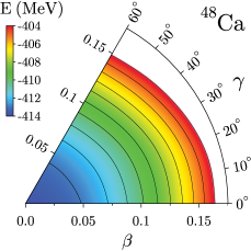
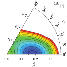
Figure 1: The particle-number projected potential energy surfaces of ⁴⁸Ca and ⁴⁸Ti in the deformation $(\beta,\gamma)$ plane for the interaction EM1.8/2.0 with $e_{\text{max}}=8$, $\hbar\omega=$16\text{\,}\mathrm{MeV}$$ (see text). Neighboring contour lines are separated by $1\text{\,}\mathrm{MeV}$.

Results and discussion.

Figure 1 displays the “potential energy surfaces,” i.e., the expectation values $\braket{\Phi_{ZN}(\bm{Q}_{i})}{\tilde{H}}{\Phi_{ZN}(\bm{Q}_{i})}$, for ⁴⁸Ca and ⁴⁸Ti. The expectation value at each deformation $(\beta,\gamma)$, where $\beta\equiv 4\pi/(3AR^{2}_{0})\sqrt{q_{0}^{2}+2q_{2}^{2}}$ with $R_{0}=1.2\,A^{1/3}\,\mathrm{fm}$ and $\gamma\equiv\arctan{\sqrt{2}q_{2}/q_{0}}$, is an indication of the importance of the corresponding state in our GCM wave functions. The IMSRG-evolved Hamiltonian $\tilde{H}$ used to construct the surface comes from the EM1.8/2.0 interaction, with $e_{\rm max}=8$ and $\hbar\omega=16$ MeV. For convenience, we use the bare rather than the evolved quadrupole operators to define $\beta$ and $\gamma$; this convention has no effect on computed observables. The figure shows that the energy of ⁴⁸Ca is minimized for a spherical shape ($\beta=0,\gamma=0$), and that the energy of ⁴⁸Ti has a similarly pronounced minimum at a prolate shape with $\beta\sim 0.2$ and $\gamma=0$. The effect of triaxiality on the low-lying states of both nuclei and on the NME is negligible.

We compute all observable quantities with the chiral interactions discussed above, for a range of $e_{\text{max}}$ and $\hbar\omega$ values (see Supplemental Material for details.) With EM1.8/2.0, which produces satisfactory ground-state and separation energies through mass $A\sim 80$ Simonis et al. (2017); Holt et al. (2019); Hagen et al. (2016); Drischler et al. (2019), we obtain extrapolated ground-state energies of -418.26 MeV and -422.27 MeV for ⁴⁸Ca and ⁴⁸Ti, respectively. Our calculation yields the correct ground-state ordering, but our $Q_{\beta\beta}$=$5.57\text{\,}\mathrm{MeV}$ is somewhat larger than the experimental $Q$ value, $4.26\text{\,}\mathrm{MeV}$.

Figure 2 shows the low-lying states of ⁴⁸Ti for the same interactions. The spectrum is clearly rotational but slightly stretched, a result of our focus on the ground state. Importantly, however, we reproduce the collective $B(\text{E2: }2_{1}^{+}\to 0_{1}^{+})$ reasonably well in all cases. Other ab initio calculations severely underpredict $B(\text{E2})$’s Parzuchowski et al. (2017); Stroberg et al. (2019), which are more sensitive probes of wave functions than are energies; our success is due to the explicit treatment of collectivity. The inclusion of noncollective configurations from isoscalar pairing, not shown in the figure, slightly compresses the spectra and changes the $B(\text{E2: }2_{1}^{+}\to 0_{1}^{+})$ by  5-6%, e.g., from $101\text{\,}{\mathrm{\text{ $e$ }}}^{2}\text{\,}{\mathrm{fm}}^{4}$ to $96\text{\,}{\mathrm{\text{ $e$ }}}^{2}\text{\,}{\mathrm{fm}}^{4}$ for the EM1.8/2.0 interaction.

The energies of the low-lying states are converged to within a few percent with respect to the basis size. For example, the $2^{+}$ excitation energies in ⁴⁸Ti obtained with EM1.8/2.0 or EM2.0/2.0 with $\hbar\omega=16$ MeV change by no more than $3\text{\,}\mathrm{\char 37\relax}$ from $e_{\text{max}}=6$ through $e_{\text{max}}=10$ (also see Supplemental Material). Regarding the transitions, we note first that the correction to the $E2$ operator from the IMSRG flow alters the $B(E2)$ values by less than 10%, suggesting that our collective reference ensemble accounts for quadrupole correlations that caused large corrections in other work Parzuchowski et al. (2017). Thus, we do not expect them to change significantly as the number of shells is increased (Fig. 4 supports our expectation). Surprisingly, even a drastic change of the coefficients ($c_{I},c_{F}$) specifying the contributions of ⁴⁸Ca and ⁴⁸Ti to the reference ensemble from $(0.5,0.5)$ to $(0.1,0.9)$ changes the ground-state energy by a mere $100$-$200\text{ keV}$, excited-state energies by 5% or less, and the $B(E2)$ by only 1%.

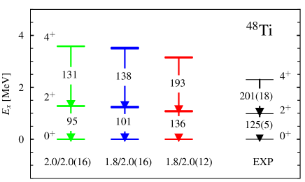
Figure 2: The low-lying energy spectrum in ⁴⁸Ti from the IMSRG+GCM calculation, with interactions and oscillator frequencies labeled EM$\lambda/\Lambda(\hbar\omega)$. The rightmost column contains experimental data National Nuclear Data Center .

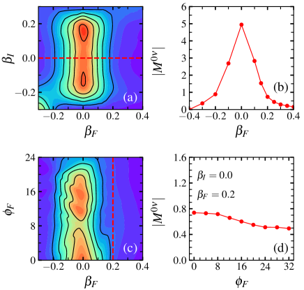
Figure 3: (a) Contributions to the NME $\lvert{M^{0\nu}}\rvert$ in the $(\beta_{I},\beta_{F})$ plane (see text). Neighboring contour lines here and in (c) are separated by $0.50$. (b) The NME $\lvert{M^{0\nu}}\rvert$ as a function of the quadrupole deformation parameter $\beta_{F}$ in ⁴⁸Ti. (c) Contributions to $\lvert{M^{0\nu}}\rvert$ in the $(\beta_{F},\phi_{F})$ plane. (d) The NME $\lvert{M^{0\nu}}\rvert$ as a function of the proton-neutron pairing amplitude $\phi_{F}$ in ⁴⁸Ti.

Table 1: The NME $M^{0\nu}$ for the decay ⁴⁸Ca $\to$ ⁴⁸Ti from the IMSRG+GCM calculation. The results labeled by */${\dagger}$ are from nonstandard reference ensembles with mixing weights $(1/3,2/3)$ and $(0.1,0.9)$, respectively. For other cases the weights are $(1/2,1/2)$.

		NME
Interaction	$\hbar\omega$	$e_{\text{max}}=6$	$e_{\text{max}}=8$	$e_{\text{max}}=10$
EM1.8/2.0	12	0.85	0.70	0.64
EM1.8/2.0	16	1.03	0.78	0.66
EM2.0/2.0	16	1.02	0.68	0.75
EM1.8/2.0∗	16		0.81
EM1.8/2.0†	16		0.80

We turn next to the $0\nu\beta\beta$ NME, which we compute with the usual form for the nuclear current operator Šimkovic et al. (2008). We neglect newly discovered corrections to the decay operator in chiral EFT Cirigliano et al. (2018a, b) and many-body currents Menéndez et al. (2011); Wang et al. (2018). Figure 3 displays NME contributions from components with different values of the generator coordinates. These contributions are multiplied by the weight functions $F$ in Eq. (2) of both the initial and final states, and then integrated to get the complete NME. Figures 3(a) and 3(b) show that the contributions hardly depend on the initial deformation $\beta_{I}$, as long as that quantity is between $-0.2$ and $0.2$, but vary strongly with the final deformation $\beta_{F}$. The significant average deformation of ⁴⁸Ti means that the NME will be suppressed. This result echoes the findings of DFT calculations, which show strong quenching of NMEs between initial and final states with different shapes Rodríguez and Martínez-Pinedo (2010); Yao et al. (2015). Figures 3(c) and 3(d) illustrate how the NME is affected by isoscalar pairing, which was shown to be significant in valence-space GCM calculations with empirical interactions Menéndez et al. (2016); Jiao et al. (2017). The ground state of ⁴⁸Ti is dominated by configurations with $\beta_{F}\approx 0.2$, and at those values the isoscalar pairing is significantly smaller than at $\beta_{F}=0$. Thus, its overall effect on the NME is mild, as panel (d) demonstrates. (Isoscalar pairing in ⁴⁸Ca is negligible.)

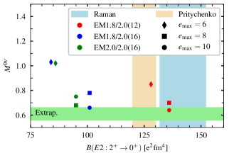
Figure 4: The NME $M^{0\nu}$ versus the $B(\text{E2: }2_{1}^{+}\to 0_{1}^{+})$ value in ⁴⁸Ti from IMSRG+GCM calculation, with different interactions, oscillator frequencies, and cutoffs. The vertical shaded areas indicate the experimental $B(\text{E2: }2_{1}^{+}\to 0_{1}^{+})$ values for ⁴⁸Ti from Refs. Raman et al. (2001); Pritychenko et al. (2016). The horizontal area represents the results ($0.61^{+0.04}_{-0.05}$) of extrapolation.

For this reason and because GCM calculations with energy density functionals find cancellations between isoscalar and isovector pairing fluctuations Vaquero et al. (2013), we present results without the isoscalar-pairing amplitude as a generator coordinate. Table 1 lists the full NMEs of both nuclei with several interactions. The results in the largest model spaces are relatively close to one another, ranging from $0.64$ to $0.75$. All results are summarized in Fig. 4. We find a noticeable but weak correlation between the NME and the $B(\text{E2: }2_{1}^{+}\to 0_{1}^{+})$ value in ⁴⁸Ti, especially in our largest model space. The weakness may reflect the relative insensitivity of the NME to the correlations at large nucleon separations that strongly affect $B(\text{E2})$’s. To extrapolate our results to even larger model spaces, we perform a Bayesian fit of the parameters in the exponential formula Basili et al. (2019) $M^{0\nu}(e_{\rm Max})=M^{0\nu}(\infty)+a\exp(-be_{\rm Max})$. For the interaction EM1.8/20 with $\hbar\omega=$16\text{\,}\mathrm{MeV}$$, we obtain an extrapolated NME of $M^{0\nu}(\infty)=0.57$, with an extrapolation uncertainty range of $(+0.08,-0.1)$; with $\hbar\omega=$12\text{\,}\mathrm{MeV}$$ we get $0.66$ with a range of $(+0.03,-0.10)$. With the constraint that the extrapolated values for both oscillator frequencies be equal, we obtain $M^{0\nu}(\infty)=0.61$ with an extrapolation uncertainty range of $(+0.04,-0.05)$. For EM2.0/2.0, the oscillation with $e_{\rm max}$ prevents a similar analysis. Our results carry additional uncertainties that will be investigated further by improving the IMSRG truncation and including isoscalar and isovector proton-neutron pairing generator coordinates, as discussed above.

All central values for our NMEs are near or below the predictions of phenomenological models Menéndez et al. (2009a); Šimkovic et al. (2013); Yao et al. (2015); Iwata et al. (2016). Only a very recent shell-model study Coraggio et al. (2020) with perturbatively derived effective interactions and operators yields an even smaller NME of 0.3. The small size of our NMEs seems to result from the interplay of valence-space and beyond valence-space correlations that our no-core approach is able to capture.

Finally, we note a significant renormalization of the NME by the IMSRG flow. With the unevolved $0\nu\beta\beta$ operator, the NME for EM1.8/2.0 at $\hbar\omega=16$ MeV and $e_{\rm max}=8$ is 0.31 instead of 0.78. A more detailed analysis shows that the flow incorporates the effects of pairing in high-energy orbitals, greatly enhancing the $J=0$ contribution to the NME. Breaking down the NME by the distance between the decaying nucleons, we confirm that the largest contribution comes from a peak around 1 fm (cf. Ref. Menéndez et al. (2009)), but contributions at larger distances are not negligible (see Supplemental Material).

Conclusions.

Ab initio methods are essential for the calculation of $0\nu\beta\beta$ matrix elements with real error estimates. We have reported the first ab initio calculation of the spectrum and transition probabilities in a deformed medium-mass nucleus, and significant progress in the ab initio computation of the NME for the $0\nu\beta\beta$ decay of ⁴⁸Ca. Our approach, based on a novel method for deformed nuclei that combines the IMSRG and GCM, has been validated in light nuclei against the no-core shell model (see Ref. Basili et al. (2019) and a forthcoming paper) and allows a systematic exploration of theoretical uncertainties. Here, we reproduce the low-lying (collective) spectrum and $E2$ transitions of ⁴⁸Ti satisfactorily. Our $B(E2)$ values are much improved compared to previous ab initio calculations Parzuchowski et al. (2017), but retain a significant dependence on $\hbar\omega$ even as we enlarge the model space. This result supports the ideas behind our method: Collective correlations that are omitted due to the IMSRG truncation can be captured by sophisticated reference states instead. Fortunately, the correlation between the NME and the $B(\text{E2})$ value is weak.

Our best estimate of the NME with EM1.8/2.0 is $M^{0\nu}=0.61$; for EM2.0/2.0 it would be a few percent larger. These values are near or below the predictions of most phenomenological approaches Engel and Menéndez (2017). Isoscalar pairing can further reduce the NME by about $17\text{\,}\mathrm{\char 37\relax}$, but the effect might be less when the calculation also includes isovector pairing fluctuations Vaquero et al. (2013).

To assign an overall error bar, we will implement improved IMSRG truncations Hergert et al. (2018); Morris (2016); Hergert et al. (2016), explore additional collective correlations with the GCM, include the (small) effects of “short-range correlations” by evolving the $0\nu\beta\beta$ operator to the same resolution scale as the interaction, and consistently treat its contributions from higher orders in chiral EFT, including many-body currents Wang et al. (2018); Gysbers et al. (2019). We must also account for a leading-order contact operator Cirigliano et al. (2018a) whose coefficient is currently unknown. We do not expect any of these steps (except perhaps the inclusion of the contact operator) to dramatically change the matrix element, and therefore plan to apply our new framework to heavier double beta decay candidate nuclei, such as ⁷⁶Ge and ¹³⁶Xe.

I Supplemental Material for: Ab Initio Treatment of Collective Correlations and the Neutrinoless Double Beta Decay of ⁴⁸Ca

J. M. Yao

B. Bally J. Engel

R. Wirth

T. R. Rodríguez

H. Hergert

II Interactions

In our calculations, we use interactions constructed in Ref. Hebeler et al. (2011), which yield an empirically reasonable description of finite nuclei and infinite nuclear matter Simonis et al. (2017); Holt et al. (2019); Drischler et al. (2019).

The two-nucleon interaction is the next-to-next-to-next-to leading order (N³LO) potential with a momentum cutoff of $\Lambda=500$MeV/$c$ constructed by Entem and Machleidt Entem and Machleidt (2003), abbreviated as EM in the present manuscript and elsewhere Hebeler et al. (2011); Simonis et al. (2017); Holt et al. (2019); Drischler et al. (2019). The resolution scale of this interaction is lowered by means of a free-space similarity renormalization group (SRG) evolution to $\lambda=$1.8\text{\,}{\mathrm{fm}}^{-1}$$ or $\lambda=$2.0\text{\,}{\mathrm{fm}}^{-1}$$, respectively Bogner et al. (2010). Following the strategy of Refs. Nogga et al. (2004); Hebeler et al. (2011), the EM interaction is supplemented with a next-to-next-to leading (N²LO order chiral three-nucleon force with cutoff $\Lambda=$2.0\text{\,}{\mathrm{fm}}^{-1}$\approx 400$ MeV/$c$ whose low-energy constants $c_{D}$ and $c_{E}$ are fit to reproduce the triton binding energy and matter radius of ${}^{4}\mathrm{He}$ (the values of the LECs $c_{1},3,4$ are the same as those used in the EM interaction). In this way, the authors of Refs. Nogga et al. (2004); Hebeler et al. (2011) aim to account for the evolution of an initial chiral 3NF to lower resolution, as well as any induced 3NFs from the evolution of the two-nucleon interaction.

III Structure properties

Table 2: The structural properties of [48]Ti from the IMSRG+GCM calculation with the chiral interactions, in comparison with available data. All energies are in units of $\mathrm{MeV}$ and $B(\text{E2})$ in ${\mathrm{\text{ $e$ }}}^{2}\text{\,}{\mathrm{fm}}^{4}$. The results with $*/\dagger$ are from the calculations starting from the ensemble reference state with mixing weight $(1/3,2/3)/(0.1,0.9)$. For other cases, $(1/2,1/2)$ is used.

EM$\lambda/\Lambda(e_{\text{max}}/\hbar\omega)$	$E(0^{+}_{1})$	$E_{x}(2^{+}_{1})$	$E_{x}(4^{+}_{1})$	$B(E2:2_{1}^{+}\to 0_{1}^{+})$
EM1.8/2.0(6/16)	-401.97	1.25	3.35	84
EM1.8/2.0(8/16)	-418.22	1.24	3.57	101
EM1.8/2.0(10/16)	-421.48	1.24	3.48	101
EM1.8/2.0(8/16)*	-417.96	1.30	3.62	99
EM1.8/2.0(8/16)$\dagger$	-418.32	1.32	3.71	100
EM1.8/2.0(6/12)	-387.68	1.03	2.90	128
EM1.8/2.0(8/12)	-409.65	1.06	3.10	136
EM1.8/2.0(10/12)	-416.95	1.08	3.14	137
EM2.0/2.0(6/16)	-361.59	1.32	3.48	86
EM2.0/2.0(8/16)	-387.18	1.33	3.63	95
EM2.0/2.0(10/16)	-395.34	1.28	3.58	95
Exp.	-418.70	0.98	2.30	144 Raman et al. (2001)
				125 Pritychenko et al. (2016)

Table 2 lists the detailed information on the low-lying states of [48]Ti from IMSRG+GCM calculations by mixing axially deformed configurations. One can see that the low-energy spectra (except for the ground-state energies) and E2 transition strengths are converged rather well at $e_{\text{max}}=10$.

Figure 5 shows the energy surfaces of [48]Ca and [48]Ti in the $(\beta_{2},\phi_{np})$ plane from the calculation using the EM1.8/2.0 interaction. It is seen clearly that the energy minimum is located at $\beta_{2}=0.0$ and $\beta_{2}=0.2$ for [48]Ca and [48]Ti, respectively. Besides, the energy surface is rather soft along the neutron-proton isoscalar pairing amplitude $\phi_{np}$ in both nuclei around the energy minimum. Therefore, the wave functions of their ground states, which are relevant for the NME of the $0\nu\beta\beta$, are mainly concentrated along the the valley, as illustrated in Fig. 6. We note that the inclusion of $\phi_{np}$ degree-of-freedom only changes slightly the energies of low-lying states. For [48]Ca, the ground-state energy is changed from -413.86 MeV to -413.87 MeV by the EM1.8/2.0 interaction with $e_{\text{max}}=8$ and $\hbar\omega=16$ MeV. For [48]Ti, it is changed from -418.22 MeV to -418.23 MeV. This effect decreases the excitation energy of $2^{+}$ state from 1.24 MeV to 1.17 MeV, closer to the data. Figure 7 shows the convergence behavior of the ground-state energies as a function of the $e_{\text{max}}$. The results are extrapolated with the exponential formula $E(e_{\rm Max})=E(\infty)+a\exp(-b\cdot e_{\rm Max})$. We find $E(\infty)=-418.26$ MeV for [48]Ca and $-422.27$ MeV for [48]Ti.

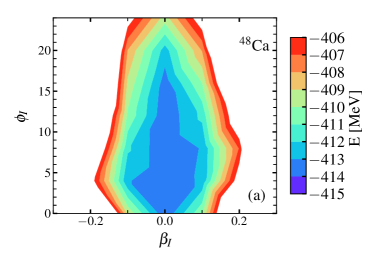
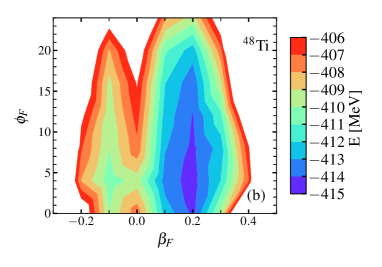
Figure 5: The particle-number projected potential energy surfaces of [48]Ca and [48]Ti in the $(\beta_{2},\phi_{np})$ plane at $e_{\rm max}=8$, $\hbar\omega=16$ MeV. The two neighbouring contour lines are separated by 1.0 MeV.

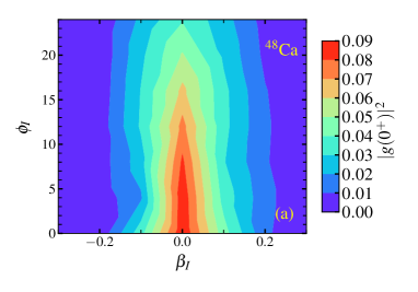
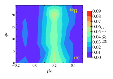
Figure 6: The collective wave functions of the ground state for [48]Ca and [48]Ti in the $(\beta_{2},\phi_{np})$ plane at $e_{\rm max}=8$, $\hbar\omega=16$ MeV. The two neighbouring contour lines are separated by 0.01.

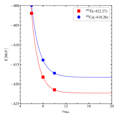
Figure 7: The ground-state energy from the IMSRG+GCM calculation with the EM1.8/2.0 interaction with oscillator frequency $\hbar\omega=$16\text{\,}\mathrm{MeV}$$ as a function of $e_{\text{max}}$.

IV IMSRG-Evolved Neutrinoless Double Beta Decay Operator

In the IMSRG flow, the evolved $0\nu\beta\beta$ decay operator is calculated with the BCH formula,

$$O^{0\nu}(s)=O^{0\nu}+[\Omega(s),O^{0\nu}]+\dfrac{1}{2}[\Omega(s),[\Omega(s),O^{0\nu}]]+\cdots$$ (3)

The leading-order correction $[\Omega(s),O^{0\nu}]$ is illustrated schematically with Goldstone diagrams in Fig. 8. The correction from this term to the operator goes to all the terms in the BCH formula. We find that the contribution from the one-body part (first two columns in Fig. 8) of $\Omega(s)$ to the commutator $[\Omega(s),O^{0\nu}]$ is negligible. The contribution of the diagrams in the third and four columns enhances the two-body matrix elements, while that of the last column quenches the matrix elements.

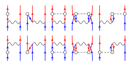
Figure 8: Antisymmetrized Goldstone diagrams of the leading-order correction $[{\Omega},{O^{0\nu}}]$ from the IMSRG evolution to the $0\nu\beta\beta$ decay operator. Hollow dots mark insertions of one- or two-body parts of $\Omega$, wavy lines correspond to $O^{0\nu}$. The diagrams in the bottom row have to be subtracted. Diagrams containing two-body cumulants cancel and have been omitted. Formulas can be found in Ref. Yao et al. (2018).

V Configuration-Dependence of the Nuclear Matrix Element

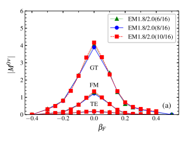
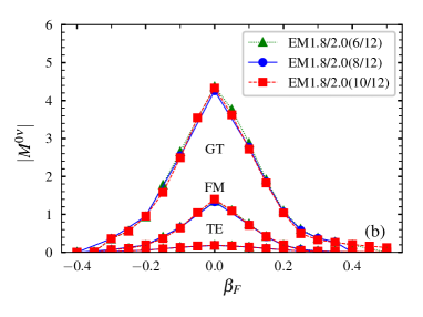
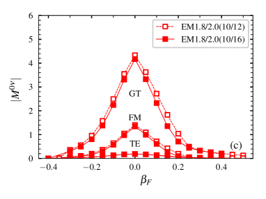
Figure 9: (a) The normalized NME $M^{0\nu}$ from the spherical state of [48]Ca to different axially deformed state of [48]Ti from the IMSRG+GCM calculation using EM1.8/2.0($e_{\text{max}}/16$) with $e_{\text{max}}=6,8,$ and 10, respectively; (b) Same as (a) but by the EM1.8/2.0($e_{\text{max}}/12$) ; (c) Comparison of the results by EM1.8/2.0($10/12$) and EM1.8/2.0($10/16$).

Figure 9 displays that the NME is very sensitive to the quadrupole deformation of [48]Ti, but not much to the $e_{\text{max}}$ for a given deformed state with the same $\beta^{(F)}_{2}$ value. Moreover, one can see that the NME by $\hbar\omega=12$ MeV is systematically larger than that by $\hbar\omega=16$ MeV. However, as we find, the $E2$ transition strengths by the former is also systematically larger than the later. Because of negative correlation between the NME and $E2$ transition strength, these two interactions predicts a similar value for the NME in the final IMSRG+GCM calculation.

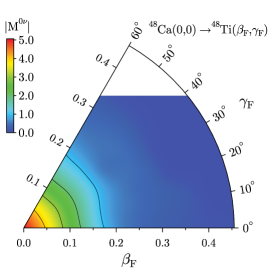
Figure 10: The configuration-dependence of the NME in the $(\beta_{2},\gamma)$ plane by the EM1.8/2.0(8/16) calculation.

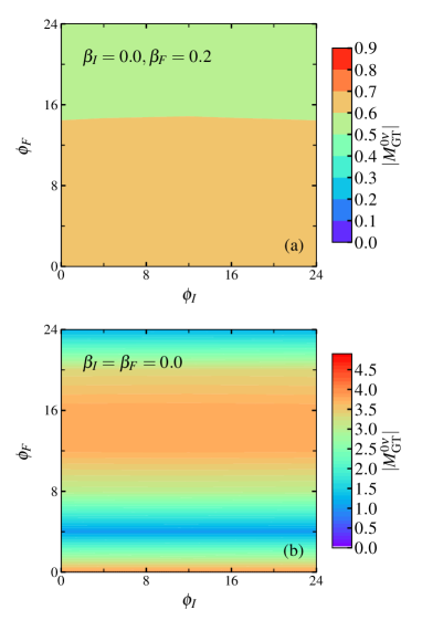
Figure 11: The configuration-dependence of the NME in the $(\phi^{(I)}_{\rm np},\phi^{(F)}_{\rm np})$ plane at $e_{\rm max}=8$, $\hbar\omega=16$ MeV.

Table 3: The nuclear matrix element $M^{0\nu}$ for the $0\nu\beta\beta$ [48]Ca $\to$ [48]Ti from the IMSRG+GCM calculation without ($w/o$) and with($w/$) the neutron-proton isoscalar pairing fluctuation using the EM1.8/2.0 interaction and $\hbar\omega=16$ MeV. The quenching factor $q$ is defined as the ratio of the difference in the NMEs to that without $np$ isoscalar pairing.

$e_{\text{max}}$	$M^{0\nu}(w/o)$	$M^{0\nu}(w/)$	$q$
6	1.03	0.86	16.5%
8	0.78	0.65	16.7%

Figure 10 shows that the NME is insensitive to the triaxial $\gamma$ deformation of [48]Ti. The inclusion of triaxiality in the GCM calculation is thus expected to be negligible. Figure 11 displays the sensitivity of the NME to the neutron-proton isoscalar pairing amplitude $\phi_{\rm np}$ in both initial and final nuclei for a given quadrupole deformation parameter. It is seen that the NME is almost independent of $\phi^{(I)}_{\rm np}$ in [48]Ca, but may vary rapidly with $\phi^{(F)}_{\rm np}$ in [48]Ti, depending on the $\beta^{(F)}_{2}$.

Table 3 lists the NME from the IMSRG+GCM calculation with neutron-proton isoscalar pairing fluctuation with $e_{\text{max}}=6$ and 8. Compared with the value from the same calculation but without the isoscalar pairing fluctuation, this value is smaller by about 17% in both cases.

VI Distance- and Angular-Momentum Dependence of the NME

We can analyze the NME further by breaking it down into contributions from different distances between the decaying nucleons and partial waves. For the former, we introduce the distribution $C^{0\nu}(r_{12})$, defined by

$$M^{0\nu}=\int^{\infty}_{0}\mathrm{d}r_{12}\,C^{0\nu}(r_{12})\,,$$ (4)

with $r_{12}=|\bm{r}_{1}-\bm{r}_{2}|$ the relative distance between the two neutrons that are transformed into protons.

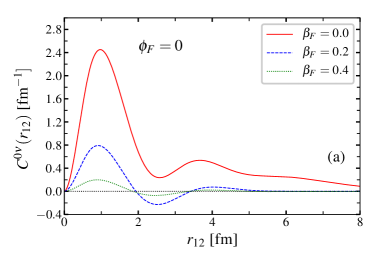
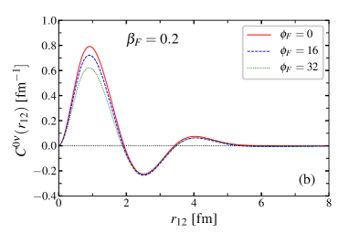
Figure 12: The distribution of $C^{0\nu}(r_{12})$ as a function of the relative coordinate $r_{12}$ corresponding to the transition from spherical [48]Ca to different configuration of [48]Ti by EM1.8/2.0(8/16) distinguished with different values of quadrupole deformation parameter $\beta_{2}$ and neutron-proton isoscalar pairing amplitude $\phi_{np}$.

Figure 12 shows distributions of the NME corresponding to the transition from spherical [48]Ca to [48]Ti with different quadrupole deformation and isoscalar pairing amplitude. One can see that the quadrupole correlation quenches the NME in both the long-ranged and short-ranged region. In contrast, the isoscalar pairing quenches the NME mainly in the short-ranged region. The distributions with deformed final states are qualitatively similar to those obtained in phenomenological shell-model calculation of Ref. Menéndez et al. (2009), featuring the appearance of a robust node at $r_{12}\approx$2.0\text{\,}\mathrm{fm}$$.

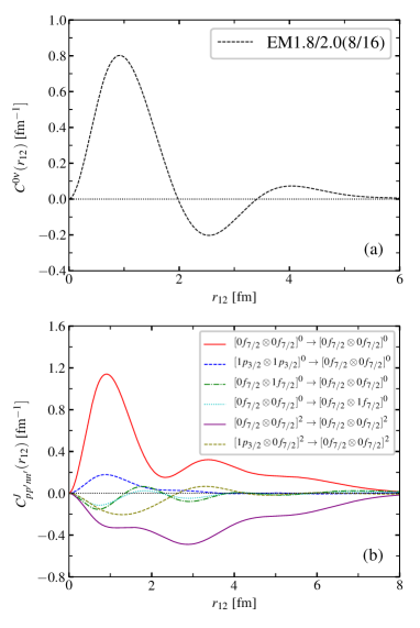
Figure 13: (a) The distribution of $C^{0\nu}(r_{12})$ as a function of the relative coordinate $r_{12}$ from the IMSRG+GCM calculation by EM1.8/2.0(8/16). (b) The contribution from the first six largest two-body transition densities.

We decompose the $C^{0\nu}(r_{12})$ further into different $J$ components

$$C^{0\nu}(r_{12}) =\sum_{\begin{subarray}{c}p\leq p^{\prime}\\ n\leq n^{\prime}\end{subarray}}\sum_{J}C^{J}_{pp^{\prime}nn^{\prime}}(r_{12}),$$ (5)

where

$$C^{J}_{pp^{\prime}nn^{\prime}}(r_{12}) =\dfrac{(2J+1)}{\sqrt{(1+\delta_{pp^{\prime}})(1+\delta_{nn^{\prime}})}}$$

$$\phantom{{}={}}\times\braket{(pp^{\prime})J}{\bar{O}^{0\nu}(r_{12})}{(nn^{\prime})J}\rho^{J}_{pp^{\prime}nn^{\prime}},$$ (6)

with $\braket{(pp^{\prime})J}{\bar{O}^{0\nu}(r_{12})}{(nn^{\prime})J}$ being the normalized IMSRG evolved two-body transition matrix element in harmonic-oscillator basis and the two-body transition density

$$\rho^{J}_{pp^{\prime}nn^{\prime}}=-\dfrac{1}{\sqrt{2J+1}}\braket{\Psi(\nuclide[48]{Ti})}{[a^{\dagger}_{p}a^{\dagger}_{p^{\prime}}]^{J}[\tilde{a}_{n}\tilde{a}_{n^{\prime}}]^{J}}{\Psi(\nuclide[48]{Ca})}.$$ (7)

Figure 13 displays the $r$-dependence of the $C^{J}_{pp^{\prime}nn^{\prime}}(r_{12})$ from the first six largest two-body transition densities. It is seen that the cancellation between $J=0$ and $J=2$ components is the main mechanism responsible for the node around $r_{12}=$2.0\text{\,}\mathrm{fm}$$, before and after which point the contribution to the total NME is opposite. It is the large negative contribution from the $J=2$ components arising from the strong quadrupole collectivity in [48]Ti quenches the NME strongly.

VII Extrapolation to Infinite Model Space

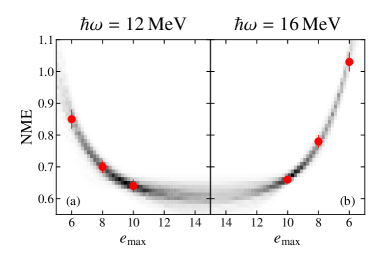
Figure 14: The NME $M^{0\nu}$ from the IMSRG+GCM calculation with the EM1.8/2.0 interaction with oscillator frequencies $\hbar\omega=$12\text{\,}\mathrm{MeV}$$ and $\hbar\omega=$16\text{\,}\mathrm{MeV}$$ as a function of $e_{\text{max}}$. The histogram in the background shows the density of 500 realizations of the extrapolating curve drawn from its posterior distribution. Both curves are constrained to yield the same extrapolated value.

To get a reliable estimate of the NME extrapolated to infinite model space and its error in the presence of uncertainty in the calculation results, we perform Bayesian inference on the parameters of the exponential formula $M^{0\nu}(e_{\rm Max})=M^{0\nu}(\infty)+a\exp(-b\cdot e_{\rm Max})$. The results are displayed in Figure 14. We use normal priors for the extrapolated value ($\mu=0.5$, $\sigma=1$) and for the value at $e_{\text{max}}=6$, where the expectation value is set to the central value of the calculation result and we set $\sigma=0.2$ to allow for some variation in the extrapolating curve. The prior for the decay constant is a truncated normal distribution ($\mu=0.5$, $\sigma=2$) with the probability density for values less than zero removed in order to get a decaying exponential. We assume Gaussian uncertainties on the resulting values of the NME.

First, we perform inference separately on the $e_{\text{max}}$ sequences for both oscillator frequencies. The uncertainty on the value of the NME at finite $e_{\text{max}}$ allows for two solutions, one with a large decay constant and an extrapolated value in the region of $0.6$, and one with a small decay constant and very low extrapolated value. This leads to a posterior distribution of the extrapolated value with a very long tail ranging into negative NME values. However, the bulk of the probability is concentrated in a rather small interval. For these reasons, we use the mode of the posterior as a point estimate and the $68\text{\,}\mathrm{\char 37\relax}$ highest posterior density credible interval to define its uncertainty. For $\hbar\omega=$16\text{\,}\mathrm{MeV}$$, we get an extrapolated value of $0.57$ with an extrapolation uncertainty range of $(+0.08,-0.1)$, the result for $\hbar\omega=$12\text{\,}\mathrm{MeV}$$ is $0.66$ with extrapolation uncertainty range $(+0.03,-0.1)$. To improve upon this and to get rid of the long tails in the posterior distribution, we also perform a combined fit where the extrapolated value is constrained to be the same for both oscillator frequencies while the other parameters are independent. The inference on the combined data set yields a much more narrow distribution of the extrapolated value and reduces the probability of the slowly decaying solutions. The extrapolated value in this case is $0.61$ with an extrapolation uncertainty range $(+0.04,-0.05)$.

References

- Fukuda et al. (1998) Y. Fukuda et al. (Super-Kamiokande Collaboration), Phys. Rev. Lett. 81, 1562 (1998).
- Ahmad et al. (2001) Q. R. Ahmad, , et al. (SNO Collaboration), Phys. Rev. Lett. 87, 071301 (2001).
- Eguchi et al. (2003) K. Eguchi, , et al. (KamLAND Collaboration), Phys. Rev. Lett. 90, 021802 (2003).
- An et al. (2012) F. P. An et al. (Daya Bay Collaboration), Phys. Rev. Lett. 108, 171803 (2012).
- Furry (1939) W. H. Furry, Phys. Rev. 56, 1184 (1939).
- Kotila and Iachello (2012) J. Kotila and F. Iachello, Phys. Rev. C 85, 034316 (2012).
- Stoica and Mirea (2013) S. Stoica and M. Mirea, Phys. Rev. C 88, 037303 (2013).
- Šimkovic et al. (2018) F. Šimkovic, R. Dvornický, D. Štefánik, and A. Faessler, Phys. Rev. C 97, 034315 (2018).
- Šimkovic et al. (2008) F. Šimkovic, A. Faessler, V. Rodin, P. Vogel, and J. Engel, Phys. Rev. C 77, 045503 (2008).
- Engel and Menéndez (2017) J. Engel and J. Menéndez, Rep. Prog. Phys. 80, 046301 (2017).
- Navrátil et al. (2009) P. Navrátil, S. Quaglioni, I. Stetcu, and B. R. Barrett, J. Phys. G 36, 083101 (2009).
- Lee (2009) D. Lee, Prog. Part. Nucl. Phys. 63, 117 (2009).
- Barrett et al. (2013) B. R. Barrett, P. Navrátil, and J. P. Vary, Prog. Part. Nucl. Phys. 69, 131 (2013).
- Launey et al. (2016) K. D. Launey, T. Dytrych, and J. P. Draayer, Prog. Part. Nucl. Phys. 89, 101 (2016).
- Somà et al. (2014) V. Somà, C. Barbieri, and T. Duguet, Phys. Rev. C 89, 024323 (2014).
- Hagen et al. (2014) G. Hagen, T. Papenbrock, M. Hjorth-Jensen, and D. J. Dean, Rep. Prog. Phys. 77, 096302 (2014).
- Hergert et al. (2016) H. Hergert, S. K. Bogner, T. D. Morris, A. Schwenk, and K. Tsukiyama, Memorial Volume in Honor of Gerald E. Brown, Phys. Rep. 621, 165 (2016).
- Hergert (2016) H. Hergert, Physica Scripta 92, 023002 (2016).
- Stroberg et al. (2019) S. R. Stroberg, H. Hergert, S. K. Bogner, and J. D. Holt, Annu. Rev. Nucl. Part. Sci. 69, 307 (2019).
- Carlson et al. (2015) J. Carlson, S. Gandolfi, F. Pederiva, S. C. Pieper, R. Schiavilla, K. E. Schmidt, and R. B. Wiringa, Rev. Mod. Phys. 87, 1067 (2015).
- Lynn et al. (2019) J. E. Lynn, I. Tews, S. Gandolfi, and A. Lovato, Annu. Rev. Nucl. Part. Sci. 69, 279 (2019).
- Shen et al. (2019) S. Shen, H. Liang, W. H. Long, J. Meng, and P. Ring, Prog. Part. Nucl. Phys. 109, 103713 (2019).
- Pastore et al. (2018) S. Pastore, J. Carlson, V. Cirigliano, W. Dekens, E. Mereghetti, and R. B. Wiringa, Phys. Rev. C 97, 014606 (2018).
- Griffin and Wheeler (1957) J. J. Griffin and J. A. Wheeler, Phys. Rev. 108, 311 (1957).
- Ring and Schuck (1980) P. Ring and P. Schuck, The Nuclear Many-Body Problem (Springer-Verlag, New York, 1980).
- Bender and Heenen (2008) M. Bender and P.-H. Heenen, Phys. Rev. C 78, 024309 (2008).
- Yao et al. (2010) J. M. Yao, J. Meng, P. Ring, and D. Vretenar, Phys. Rev. C 81, 044311 (2010).
- Rodríguez and Egido (2010) T. R. Rodríguez and J. L. Egido, Phys. Rev. C 81, 064323 (2010).
- Yao et al. (2018) J. M. Yao, J. Engel, L. J. Wang, C. F. Jiao, and H. Hergert, Phys. Rev. C 98, 054311 (2018).
- Basili et al. (2019) R. A. M. Basili, J. M. Yao, J. Engel, H. Hergert, M. Lockner, P. Maris, and J. P. Vary, arXiv:1909.06501 [nucl-th] .
- Iida et al. (2016) T. Iida et al., J. Phys. Conf. Ser. 718, 062026 (2016).
- Entem and Machleidt (2003) D. R. Entem and R. Machleidt, Phys. Rev. C 68, 041001(R) (2003).
- Bogner et al. (2010) S. Bogner, R. Furnstahl, and A. Schwenk, Prog. Part. Nucl. Phys. 65, 94 (2010).
- Hebeler et al. (2011) K. Hebeler, S. K. Bogner, R. J. Furnstahl, A. Nogga, and A. Schwenk, Phys. Rev. C 83, 031301(R) (2011).
- Nogga et al. (2004) A. Nogga, S. K. Bogner, and A. Schwenk, Phys. Rev. C 70, 061002(R) (2004).
- Hergert et al. (2018) H. Hergert, J. M. Yao, T. D. Morris, N. M. Parzuchowski, S. K. Bogner, and J. Engel, J. Phys. Conf. Ser. 1041, 012007 (2018).
- Parzuchowski et al. (2017) N. M. Parzuchowski, S. R. Stroberg, P. Navrátil, H. Hergert, and S. K. Bogner, Phys. Rev. C 96, 034324 (2017).
- Morris et al. (2015) T. D. Morris, N. M. Parzuchowski, and S. K. Bogner, Phys. Rev. C 92, 034331 (2015).
- Stroberg et al. (2017) S. R. Stroberg, A. Calci, H. Hergert, J. D. Holt, S. K. Bogner, R. Roth, and A. Schwenk, Phys. Rev. Lett. 118, 032502 (2017).
- Kutzelnigg and Mukherjee (1997) W. Kutzelnigg and D. Mukherjee, J. Chem. Phys. 107, 432 (1997).
- Mukherjee (1997) D. Mukherjee, Chem. Phys. Lett. 274, 561 (1997).
- Menéndez et al. (2016) J. Menéndez, N. Hinohara, J. Engel, G. Martínez-Pinedo, and T. R. Rodríguez, Phys. Rev. C 93, 014305 (2016).
- Hinohara and Engel (2014) N. Hinohara and J. Engel, Phys. Rev. C 90, 031301(R) (2014).
- Bender et al. (2009) M. Bender, T. Duguet, and D. Lacroix, Phys. Rev. C 79, 044319 (2009).
- Duguet et al. (2009) T. Duguet, M. Bender, K. Bennaceur, D. Lacroix, and T. Lesinski, Phys. Rev. C 79, 044320 (2009).
- Simonis et al. (2017) J. Simonis, S. R. Stroberg, K. Hebeler, J. D. Holt, and A. Schwenk, Phys. Rev. C 96, 014303 (2017).
- Holt et al. (2019) J. D. Holt, S. R. Stroberg, A. Schwenk, and J. Simonis, arXiv:1905.10475 [nucl-th] .
- Hagen et al. (2016) G. Hagen, G. R. Jansen, and T. Papenbrock, Phys. Rev. Lett. 117, 172501 (2016).
- Drischler et al. (2019) C. Drischler, K. Hebeler, and A. Schwenk, Phys. Rev. Lett. 122, 042501 (2019).
- (50) National Nuclear Data Center, NuDat 2 Database, https://www.nndc.bnl.gov/nudat2.
- Cirigliano et al. (2018a) V. Cirigliano, W. Dekens, J. de Vries, M. L. Graesser, E. Mereghetti, S. Pastore, and U. van Kolck, Phys. Rev. Lett. 120, 202001 (2018a).
- Cirigliano et al. (2018b) V. Cirigliano, W. Dekens, E. Mereghetti, and A. Walker-Loud, Phys. Rev. C 97, 065501 (2018b).
- Menéndez et al. (2011) J. Menéndez, D. Gazit, and A. Schwenk, Phys. Rev. Lett. 107, 062501 (2011).
- Wang et al. (2018) L.-J. Wang, J. Engel, and J. M. Yao, Phys. Rev. C 98, 031301(R) (2018).
- Rodríguez and Martínez-Pinedo (2010) T. R. Rodríguez and G. Martínez-Pinedo, Phys. Rev. Lett. 105, 252503 (2010).
- Yao et al. (2015) J. M. Yao, L. S. Song, K. Hagino, P. Ring, and J. Meng, Phys. Rev. C 91, 024316 (2015).
- Jiao et al. (2017) C. F. Jiao, J. Engel, and J. D. Holt, Phys. Rev. C 96, 054310 (2017).
- Vaquero et al. (2013) N. L. Vaquero, T. R. Rodríguez, and J. L. Egido, Phys. Rev. Lett. 111, 142501 (2013).
- Raman et al. (2001) S. Raman, C. W. Nestor, and P. Tikkanen, At.Data Nucl.Data Tables 78, 1 (2001).
- Pritychenko et al. (2016) B. Pritychenko, M. Birch, B. Singh, and M. Horoi, At.Data Nucl.Data Tables 107, 1 (2016).
- Menéndez et al. (2009a) J. Menéndez, A. Poves, E. Caurier, and F. Nowacki, Nucl. Phys. A 818, 139 (2009a).
- Šimkovic et al. (2013) F. Šimkovic, V. Rodin, A. Faessler, and P. Vogel, Phys. Rev. C 87, 045501 (2013).
- Iwata et al. (2016) Y. Iwata, N. Shimizu, T. Otsuka, Y. Utsuno, J. Menéndez, M. Honma, and T. Abe, Phys. Rev. Lett. 116, 112502 (2016).
- Coraggio et al. (2020) L. Coraggio, A. Gargano, N. Itaco, R. Mancino, and F. Nowacki, Phys. Rev. C 101, 044351 (2020).
- Menéndez et al. (2009b) J. Menéndez, A. Poves, E. Caurier, and F. Nowacki, Nuclear Physics A 818, 139 (2009b).
- Morris (2016) T. D. Morris, Systematic Improvements of Ab Initio In-Medium Similarity Renormalization Group Calculations, Ph.D. thesis, Michigan State University, 2016.
- Gysbers et al. (2019) P. Gysbers, G. Hagen, J. D. Holt, G. R. Jansen, T. D. Morris, P. Navrátil, T. Papenbrock, S. Quaglioni, A. Schwenk, S. R. Stroberg, and K. A. Wendt, Nat. Phys. 15, 428 (2019).

References

- Hebeler et al. (2011) K. Hebeler, S. K. Bogner, R. J. Furnstahl, A. Nogga, and A. Schwenk, Phys. Rev. C 83, 031301(R) (2011).
- Simonis et al. (2017) J. Simonis, S. R. Stroberg, K. Hebeler, J. D. Holt, and A. Schwenk, Phys. Rev. C 96, 014303 (2017).
- Holt et al. (2019) J. D. Holt, S. R. Stroberg, A. Schwenk, and J. Simonis, (2019), arXiv:1905.10475 [nucl-th] .
- Drischler et al. (2019) C. Drischler, K. Hebeler, and A. Schwenk, Phys. Rev. Lett. 122, 042501 (2019).
- Entem and Machleidt (2003) D. R. Entem and R. Machleidt, Phys. Rev. C 68, 041001(R) (2003).
- Bogner et al. (2010) S. Bogner, R. Furnstahl, and A. Schwenk, Prog. Part. Nucl. Phys. 65, 94 (2010).
- Nogga et al. (2004) A. Nogga, S. K. Bogner, and A. Schwenk, Phys. Rev. C 70, 061002(R) (2004).
- Raman et al. (2001) S. Raman, C. W. Nestor, and P. Tikkanen, At.Data Nucl.Data Tables 78, 1 (2001).
- Pritychenko et al. (2016) B. Pritychenko, M. Birch, B. Singh, and M. Horoi, At.Data Nucl.Data Tables 107, 1 (2016).
- Yao et al. (2018) J. M. Yao, J. Engel, L. J. Wang, C. F. Jiao, and H. Hergert, Phys. Rev. C 98, 054311 (2018).
- Menéndez et al. (2009) J. Menéndez, A. Poves, E. Caurier, and F. Nowacki, Nuclear Physics A 818, 139 (2009).