Probing $\Omega\Omega$ and $p\Omega$ dibaryons with femtoscopic correlations
in relativistic heavy-ion collisions

Abstract

The momentum correlation functions of baryon pairs, which reflects the baryon-baryon interaction at low energies, are investigated for multi-strangeness pairs ($\Omega\Omega$ and $N\Omega$) produced in relativistic heavy-ion collisions. We calculate the correlation functions based on an expanding source model constrained by single-particle distributions. The interaction potentials are taken from those obtained from recent lattice QCD calculations at nearly physical quark masses. Experimental measurements of these correlation functions for different system sizes will help to disentangle the strong interaction between baryons and to unravel the possible existence of strange dibaryons.

I Introduction

Either bound or resonant dibaryons provide valuable information on baryon-baryon interactions Gal:2015rev ; Clement:2016vnl . Historic example is the bound deuteron urey32:_hydrog_isotop_mass which indicates the strong tensor force in the ${}^{3}SD_{1}$ nucleon-nucleon interaction Rarita:1941zza . Similarly, observing possible dibaryons with multi-strangeness would give useful constraints on the unknown hyperon-nucleon and hyperon-hyperon interactions. The $H$-dibaryon with spin $J\!=\!0$ and $S\!=\!-2$ Jaffe:1976yi , the $N\Omega$ with $J\!=\!2$ and $S\!=\!-3$ Goldman:1987ma ; Oka:1988yq , and the $\Omega\Omega$ with $J\!=\!0$ and $S\!=\!-6$ Kopeliovich:1990pp are particularly interesting, since the Pauli blocking among valence quarks do not operate in these systems.

In recent years, ab initio calculations of baryon-baryon interactions on the basis of lattice quantum chromodynamics (LQCD) became possible near the physical quark masses. This is due to the development of advanced techniques such as the HAL QCD method HALQCD ; HALQCD:2012aa and the unified contraction algorithm Doi:2012xd . In particular, it was numerically demonstrated that the $\Omega\Omega$ interaction in the $J=0$ channel and the $N\Omega$ interaction in the $J=2$ channel are attractive enough to hold molecular-like bound states in the S-wave Gongyo:2017fjb ; Iritani:2018sra .

To study such multi-strangeness systems experimentally, high-energy heavy-ion collisions provide a unique opportunity allowing direct search via invariant mass spectrum ExHIC ; Cho:2017dcy as well as indirect search via momentum correlations Morita:2014kza ; Morita:2016auo ; Ohnishi:2016elb ; Hatsuda:2017uxk ; Cho:2017dcy . As for the latter, a ratio of the correlation functions obtained from different source sizes has been theoretically introduced and called “small-to-large (SL) ratio” Morita:2016auo . This is useful to access e.g. the strong $p\Omega$ interaction without much contamination from the Coulomb interaction at small relative momentum. Subsequently, the measurement of the momentum correlation of $p\Omega$ was conducted in Au+Au collisions at RHIC STAR:2018uho .

The main purpose of this paper is to study the pair momentum correlation functions of the dibaryon candidates, $\Omega\Omega$ and $p\Omega$, by extending our previous analysis  Morita:2016auo ; Morita:2014kza ; Ohnishi:2016elb ; Hatsuda:2017uxk ; Cho:2017dcy . We employ the latest interactions obtained from the (2+1)-flavor lattice QCD simulations with nearly physical quark masses Gongyo:2017fjb ; Iritani:2018sra . Also we use an expanding source model constrained by experimental transverse momentum spectra and multiplicities. In Sec. II, we recapitulate the general feature of the momentum correlation function in a simplified example to give an account of how the final state interaction (FSI) is translated into the pair correlations. A model for the emission source function is described in Sec. III. We give details of the potential and resultant correlation functions for $\Omega\Omega$ pairs and $p\Omega$ pairs in Sec. IV and V, respectively. Section VI is devoted to summary and concluding remarks. In Appendix A, the system size dependence of the momentum correlation for $p\Omega$ with uncertainty quantification are examined. In Appendix B, we show a comparison of the $p\Omega$ potential in Morita:2016auo with that in  Iritani:2018sra adopted in the present paper.

II Two-particle momentum correlation from final state interactions

II.1 Formalism

We briefly recapitulate the general property of the two-particle momentum correlation function with FSI. More details can be found in, e.g., Refs. Cho:2017dcy ; Lisa:2005dd .

The momentum correlation function between particles 1 and 2 with respective momenta $p_{1}$ and $p_{2}$ is defined by the ratio of two-particle spectrum $N_{12}(\bm{p}_{1},\bm{p}_{2})=E_{1}E_{2}dN_{12}/d\bm{p}_{1}d\bm{p}_{2}$ and the product of single-particle spectra $N_{i}(\bm{p}_{i})=E_{i}dN_{i}/d\bm{p}_{i}$ as

$$C(q^{\mu},P^{\mu})=\frac{N_{12}(\bm{p}_{1},\bm{p}_{2})}{N_{1}(\bm{p}_{1})N_{2}(\bm{p}_{2})},$$ (1)

with $E_{i}=\sqrt{\bm{p}_{i}^{2}+m_{i}^{2}}$ being the on-shell particle energy. The center-of-mass momentum $P$ and the generalized relative momentum $q$ are defined by

$$P^{\mu} =p_{1}^{\mu}+p_{2}^{\mu},$$ (2)

$$q^{\mu} =\frac{1}{2}\left[p_{1}^{\mu}-p_{2}^{\mu}-\frac{(p_{1}-p_{2})\cdot P}{P^{2}}P^{\mu}\right].$$ (3)

One may, in principle, measure the correlation function as a function of three independent components of the relative momentum $q^{\mu}$. Such a decomposition has been utilized to investigate expansion dynamics of the hot matter through pion correlations Lisa:2005dd . In practice, particles except for pions do not allow for such detailed study due to limited statistics. Hereafter, we consider only one-dimensional correlation function with respect to the invariant relative momentum $q=\sqrt{-q_{\mu}q^{\mu}}$. Then we can define the experimental correlation function by

$$C(q)=\frac{A_{12}(q)}{B_{12}(q)},$$ (4)

where $A_{12}(q)$ is for the number of pairs from the same event while $B_{12}(q)$ is constructed from mixed events. Eq. (4) is related to the two-particle and single-particle spectra as

$$C(q)=\frac{\displaystyle\int\frac{d\bm{p}_{1}}{E_{1}}\frac{d\bm{p}_{2}}{E_{2}}N_{12}(\bm{p}_{1},\bm{p}_{2})\delta(q-\sqrt{-q^{2}})}{\displaystyle\int\frac{d\bm{p}_{1}}{E_{1}}\frac{d\bm{p}_{2}}{E_{2}}N_{1}(\bm{p}_{1})N_{2}(\bm{p}_{2})\delta(q-\sqrt{-q^{2}})},$$ (5)

where the momentum integration should reflect the experimental momentum coverage.

The source function $S_{i}(x,\bm{p})$ is defined as the phase space distribution of the particles at freeze-out and is related to the single-particle spectrum as

$$N_{i}(\bm{p})=\int d^{4}xS_{i}(x,\bm{p}).$$ (6)

Then the two-particle spectrum from uncorrelated (chaotic) sources reads

$$N_{12} (\bm{p}_{1},\bm{p}_{2})$$

$$\simeq\int d^{4}xd^{4}yS_{1}(x,\bm{p}_{1})S_{2}(y,\bm{p}_{2})|\Psi(x,y,\bm{p}_{1},\bm{p}_{2})|^{2}$$ (7)

$$\simeq\int d^{4}xd^{4}yS_{1}(x,\bm{p}_{1})S_{2}(y,\bm{p}_{2})|\varphi(\bm{q}^{*},\bm{r}^{*})|^{2},$$ (8)

where $\Psi(x,y,\bm{p}_{1},\bm{p}_{2})$ denotes the Bethe-Salpeter amplitude describing propagations of pairs from the emission point $x$ and $y$ to the asymptotic state with momenta $\bm{p}_{1}$ and $\bm{p}_{2}$. The squared two-particle amplitude is well approximated by the relative wave function $\varphi(\bm{q}^{*},\bm{r}^{*})$ in the pair rest frame defined by $\bm{P}=0$. Here $\bm{q}^{*}$ and $\bm{r}^{*}=\bm{x}^{*}-\bm{y}^{*}$ are the spatial components of relative momentum and the relative coordinate defined in the pair rest frame, respectively. Note that $q=|\bm{q^{*}}|$ when $\bm{P}=0$. The information on the pairwise interaction is encoded in $\varphi(\bm{q}^{*},\bm{r}^{*})$ which can be obtained by solving the Schrödinger equation. The squared relative wave function $|\varphi(\bm{q}^{*},\bm{r}^{*})|^{2}$ can be viewed as a weight factor for the two-particle emission. Therefore, $N_{12}(\bm{p}_{1},\bm{p}_{2})$ reduces to the product $N_{1}(\bm{p}_{1})N_{2}(\bm{p}_{2})$ for $|\varphi(\bm{q}^{*},\bm{r}^{*})|^{2}=1$. Note that Eq. (7) is valid under the chaotic source assumption, the so-called smoothness assumption ($S_{i}(x,\bm{p})$ being smooth in the momentum space), and the negligible correlation with other particles. The validity of Eq. (8) further requires $\bm{q}^{*}$ to be small compared with the particle masses in order for $\varphi(\bm{q}^{*},\bm{r}^{*})$ to be regarded as the relative wave function. (See Refs. Femto for detailed discussion.)

If the center-of-mass coordinate and relative time are integrated, we obtain the Koonin-Pratt formula,

$$C^{(\rm KP)}(q)=\int d\bm{r}^{*}S_{12}^{\text{rel}}(\bm{r}^{*})|\varphi(\bm{q}^{*},\bm{r}^{*})|^{2},$$ (9)

where the relative source function $S_{12}^{\text{rel}}(\bm{r}^{*})$ can be viewed as the relative source distribution in the pair rest frame. The relative source function is momentum dependent when the emission point is correlated with momentum, as is the case for collective expansion.

In this paper, we adopt a parameterized model of $S_{i}(x,\bm{p})$ with hydrodynamic expansion expansion with the parameters constrained from single-particle spectra through Eq. (6). Detailed analyses of $\pi$-$\pi$ correlations at RHIC have revealed that various features of the expanding matter need to be implemented to produce the pion emitting source compatible with measurements Pratt:2008qv . Therefore, our parameterized source may be an oversimplification. On the other hand, precise shape of the source function is not crucially important in our one-dimensional correlation. Use of more realistic source functions through the implementations of state-of-the-art dynamical models will be left for future studies.

II.2 Correlations from S-wave scattering

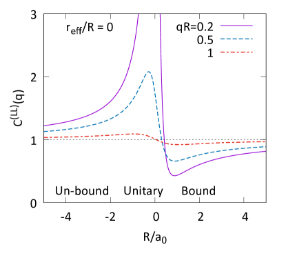
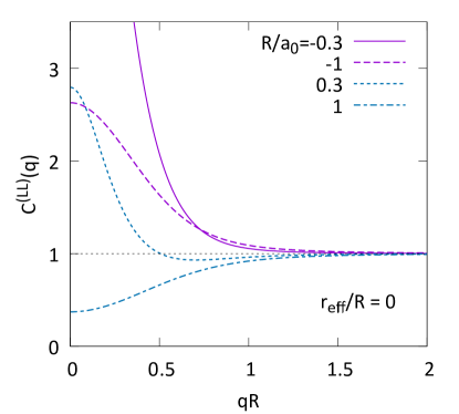
Figure 1: The correlation function $C^{(\text{LL})}(q)$ with $r_{\rm eff}=0$ as a function of $R/a_{0}$ for different $qR$ (upper panel) and as a function of $qR$ for different $R/a_{0}$ value (lower panel). In the present sign convention, $a_{0}>0$ corresponds to the existence of a bound state.

Owing to the short-range nature of the strong interaction, the modification of the relative wave function of non-identical particle pairs takes place mainly in the S-wave state. Thus, one may express

$$\varphi(\bm{q},\bm{r})=e^{i\bm{q}\cdot\bm{r}}-j_{0}(|\bm{q}|r)+\psi_{|\bm{q}|}(r),$$ (10)

where $j_{0}(x)$ is the zeroth-order spherical Bessel function, and $\psi_{|\bm{q}|}(r)$ is the S-wave relative wave function with the pairwise interaction effects. The connection of the pairwise interaction with the correlation function can be nicely illustrated by employing a static and spherically symmetric source function, $S_{12}^{\text{rel}}(\bm{r^{*}})=S(r=|\bm{r^{*}}|)$, as  Morita:2016auo

$$C^{\rm(KP)}(q)=1+\int[d\bm{r^{*}}]\left(|\psi_{q}(r)|^{2}-|j_{0}(qr)|^{2}\right),$$ (11)

where $[d\bm{r^{*}}]=d\bm{r^{*}}S(r)$ with $S(r)$ being properly normalized as $\int[d\bm{r^{*}}]=1$. One immediately finds that the deviation of the wave function from the non-interacting one is directly translated into the correlation function and that the relative source function acts as a weight factor at relative distance $r$.

Furthermore, when the source size is not too small compared to the interaction range, the integral is dominated by the contribution outside the interaction range such that the wave function can be approximated by its asymptotic form $\psi_{q}(r)\sim e^{-i\delta}\sin(qr+\delta)/(qr)$ with $\delta$ being the S-wave scattering phase shift. Employing a Gaussian source $S(r)\propto\exp(-r^{2}/4R^{2})$ and the effective range formula for small $q$,

$$q\cot\delta\simeq-\frac{1}{a_{0}}+\frac{1}{2}r_{\text{eff}}q^{2},$$ (12)

one can express the correlation function in terms of the scattering length $a_{0}$ and the effective range $r_{\text{eff}}$, which is known as the Lednický-Lyuboshits (LL) formula lednicky82:_influence ,

$$C^{(\text{LL})}(q) =1+\frac{|f(q)|^{2}}{2R^{2}}F_{3}\left(\frac{r_{\text{eff}}}{R}\right)+\frac{2\text{Re}f(q)}{\sqrt{\pi}R}F_{1}(2qR)$$

$$\quad-\frac{\text{Im}f(q)}{R}F_{2}(2qR).$$ (13)

Here $f(q)=(q\cot\delta-iq)^{-1}$ is the scattering amplitude, $F_{1}(x)=\int_{0}^{x}dte^{t^{2}-x^{2}}$, $F_{2}(x)=(1-e^{-x^{2}})/x$, and $F_{3}(x)=1-x/(2\sqrt{\pi})$. Since the scattering length dominates the behavior of the phase shift at small $q$, this correlation function is mainly determined by the scattering length and the source size: For $r_{\text{eff}}=0$, $C^{(\text{LL})}(q)$ is a function of two dimensionless variables, $qR$ and $R/a_{0}$ Cho:2017dcy .

Figure 1 represents characteristics of the correlation function $C^{(\text{LL})}(q)$ with $r_{\rm eff}=0$. For a fixed $qR$ (upper panel), the correlation function exhibits non-monotonic changes against the ratio of the system size to the scattering length. It shows a strong peak around $R/a_{0}\sim 0$ for small $qR$ due to the strong enhancement of the wave function. We call the region where $C(q)$ is enhanced as the “unitary region” throughout this paper. The peak is smeared as $qR$ is increased. As the attraction becomes weaker ($a_{0}<0$), the correlation is also weakened to exhibit monotonic decrease with decreasing $R/a_{0}$ and increasing $qR$. On the other hand, if the attraction is strong enough to accommodate a bound state ($a_{0}>0$), $C(q)$ rapidly decreases with $R/a_{0}$ then takes values less than unity implying the depletion of correlated pairs at small $qR$. The depletion can be understood by so-called the structural core; the scattering wave function needs to be orthogonal to the bound state wave function, then it has a node in the interaction range as if there is a repulsive core. Thus the squared wave function is suppressed on average.

The above properties of $C(q)$ are essential in order to extract the pairwise interaction from the measured correlation functions. In particular, the behavior of $C(q)$ for different system size provides detailed information on the scattering parameters as shown in the lower panel of Fig. 1. Consider the case where $C(q)\gg 1$ at small $qR$. It indicates that the system is in the unitary region where $|R/a_{0}|$ is small, while the sign of $a_{0}$ is unknown. However, by increasing $R$ with $a_{0}$ and $qR$ fixed, $C(q)$ eventually becomes smaller than 1 for positive $a_{0}$, while $C(q)$ is always larger than 1 for negative $a_{0}$.

In reality, the correlation at small $q$ originates not only from the single-channel FSI but also from the quantum statistics in the case of identical pairs (HBT effect), from the Coulomb interaction, and from the coupled channel effect Haidenbauer:2018jvl . Furthermore, the correlation from the HBT effect is affected by the collective flow through the modification of the source geometry. As a result, even for non-identical pairs, the absolute magnitude of $C(q)$ with respect to unity is not always a useful measure to quantify the effect of FSI in heavy-ion collisions. However, by taking a ratio of the correlation functions with small and large system sizes as

$$C_{\text{SL}}(q)=C_{\text{small-R}}(q)/C_{\text{large-R}}(q),$$ (14)

one can nicely cancel out the effect of the Coulomb interaction between charged pairs and extract the FSI from the strong interaction, as demonstrated in Morita:2016auo . We will follow this idea in this paper to study $\Omega\Omega$ and $p\Omega$ correlations.

III Modeling emission function

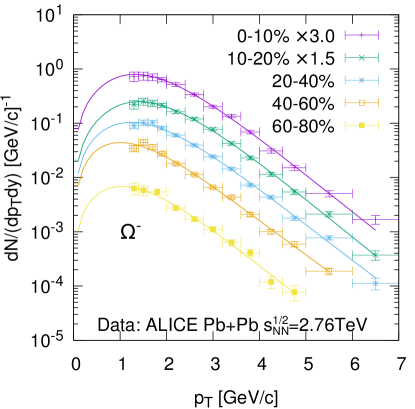
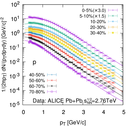
Figure 2: Transverse momentum spectra of $\Omega$ (upper) and $p$ (lower). Experimental data are taken from ABELEV:2013zaa and Abelev:2013vea for $\Omega$ and protons, respectively. Two most central events are scaled by factor 3 and 1.5 for better comparison.

As seen from Fig. 1, the correlation from FSI strongly depends on the source size. In order to extract the pairwise interaction from the correlation function, one needs to know the source size or to look at the system size dependence of the correlation Morita:2016auo . Therefore, modeling the particle source is one of the indispensable ingredients in quantitative analyses. Here, we employ a thermal source model with hydrodynamic expansion in which parameters are so tuned as to reproduce relevant particle yields and spectra.

We assume that the baryon production takes place at chemical and thermal freeze-out temperature $T_{f}$ from a cylindrically expanding boost-invariant fireball, where the flow velocity $u^{\mu}(x)$ is parameterized as $u^{\mu}=(\cosh\eta_{s}\cosh y_{T},\sinh y_{T}\cos\phi,\sinh y_{T}\sin\phi,\sinh\eta_{s}\cosh y_{T})$ with $\eta_{s}=\tanh^{-1}(z/t)$ being the spacetime rapidity. The transverse rapidity $y_{T}$ is parameterized as $y_{T}=\alpha(r_{T}/R_{T})^{\beta}$, where $\alpha$ are $\beta$ are the fitting parameters and $R_{T}$ denotes the transverse source size. Then the emission function of particle species $i$ can be written as expansion

$$d^{4}xS_{i}(x,\bm{p})=\tau_{0}d\eta_{s}d^{2}r_{T}\frac{d}{(2\pi)^{3}}n_{\text{F}}(u\cdot p,T)\exp\left(-\frac{r_{T}^{2}}{2R_{T}^{2}}\right),$$ (15)

where $\bm{p}$ is the on-shell momentum, $x$ is the spacetime emission point, $d$ denotes the spin degeneracy, and $n_{\text{F}}$ denotes the Fermi distribution function. We assume that hadrons are produced at a constant proper time $\tau=\sqrt{t^{2}-z^{2}}=\tau_{0}$ with a Gaussian profile in the transverse direction. The use of azimuthally symmetric profile is an oversimplification since it does not account for the significant anisotropic flow in non-central events, but we retain it in order to reduce the number of parameters. In fact, the one-dimensional baryon-baryon correlation functions are not expected to be strongly sensitive to detailed source shape in the transverse plane, since it can be expressed in terms of relative source distribution (9). By integrating over $\eta_{s}$ and $r_{T}$, one obtains the single particle spectrum, $EdN/d^{3}\bm{p}$. In the Boltzmann approximation $m\gg T$, the thermal spectrum is proportional to the volume factor $V=2\pi\tau_{0}R_{T}^{2}$, so that we have

$$\frac{dN}{dyp_{T}dp_{T}2\pi} =\frac{d}{(2\pi)^{3}}2m_{T}V\int_{0}^{\infty}d\rho e^{-\rho^{2}/2}$$

$$\quad\times I_{0}\left(\frac{p_{T}}{T}\sinh y_{T}\right)K_{1}\left(\frac{m_{T}}{T}\cosh y_{T}\right),$$ (16)

where $I_{0}$ and $K_{1}$ are the modified Bessel functions.

The parameters in our model are determined by the following procedure. First, we fix the freeze-out temperature to $T_{f}=155$ MeV from the fit to the various particle multiplicity data at LHC Andronic:2017pug . We perform a fit to the experimental transverse momentum spectra of each species by varying three parameters ($V,\alpha$ and $\beta$). Finally we fix $\tau_{0}=10$ fm/$c$ from a freeze-out temperature in a hydrodynamic model calculation Zhu:2015dfa for the most central event bin (5-10%) in $\Omega$ production analyses ABELEV:2013zaa . We take the relation $\tau_{0}\simeq(dN/dy)^{1/3}$ which is expected from the property of longitudinal HBT radii $R_{\text{long}}\simeq\tau_{0}\sqrt{T_{f}/m_{T}}$ Makhlin:1987gm and well-established relation between the HBT radii and multiplicity. Then $R$ is obtained from the fitted values of the volume factor $V$.

Fig.2 displays the fitted transverse momentum spectra for $\Omega$s and protons. The obtained parameter sets are summarized in Table 1. We take into account two-body decay contributions from resonances with mass $m_{R}<2$ GeV to the proton spectra. We note that those resonance contributions are important to fit the total yield of protons with reasonable system sizes. Note also that there is so-called thermal proton yield anomaly at LHC Andronic:2017pug . (See Ref. Andronic:2018qqt for a possible resolution.) The proton spectra have more detailed centrality bins than those of the $\Omega$, such that fits are made for those data. In the calculations of the correlation function below, we adjust the centrality selections to $\Omega$ data. Thus, the parameters shown in Table 1 are those used in the subsequent calculations and are obtained by averaging over corresponding centralities in the spectrum. (i.e., 0-10% parameters are obtained by averaging 0-5% and 5-10% with multiplicity being the weight.) Clearly, the present model is too simple to fully account for other possible contributions to the proton spectrum such as rescattering effect after chemical freeze-out. Nevertheless, we have checked that proton HBT radii from the model are consistent with measurements Adam:2015vja . Therefore, we expect the following results remain valid for more realistic modeling of the particle sources.

Table 1: Parameters in the emission function (15) for different centralities and particle species.

Centrality	$\tau_{0}$ [fm/$c$]	$R_{T}^{\Omega}$ [fm]	$R_{T}^{p}$	$\alpha^{\Omega}$	$\beta^{\Omega}$	$\alpha^{p}$	$\beta^{p}$
$0-10\%$	10.0	8.0	6.8	0.584	0.628	0.759	0.421
$10-20\%$	9.085	6.75	6.23	0.618	0.579	0.750	0.425
$20-40\%$	7.5	5.88	5.2	0.546	0.692	0.707	0.466
$40-60\%$	5.5	4.38	3.92	0.444	0.858	0.604	0.6
$60-80\%$	3.62	2.12	2.66	0.456	0.812	0.456	0.82

IV $\Omega\Omega$ correlation

First we discuss pairs of $\Omega(1672)$ particles. A recent LQCD calculation shows that the $J=0$ $\Omega\Omega$ system has a shallow bound state Gongyo:2017fjb . Direct detection of the $\Omega\Omega$ dibaryons (di-Omega) is highly challenging because of the tiny production rate for the $S=-6$ object even in heavy-ion collisions and the background yields of the decay products would be high. On the other hand, the high luminosity upgrade at the LHC may allow for measuring the momentum correlation of $\Omega\Omega$ pairs in the future.

IV.1 $\Omega\Omega$ interaction from lattice QCD

Since $\Omega$ has a spin $3/2$, the $\Omega\Omega$ pairs can have $J=0,1,2$ and 3. Among others, the $J=0$ state is expected to have appreciable S-wave attraction without suffering from the Pauli exclusion effect for valence quarks. The interaction potential $V_{\Omega\Omega}^{J=0}$ was recently calculated by (2+1)-flavor lattice QCD simulations Gongyo:2017fjb with a large lattice volume (8.1 fm)³, a small lattice spacing $a\simeq$ 0.0846 fm and nearly physical quark masses ($m_{\pi}\simeq$ 146 MeV, $m_{K}\simeq$525 MeV, $m_{N}\simeq$964 MeV, and $m_{\Omega}\simeq$1712 MeV). In the time-dependent HAL QCD method  HALQCD:2012aa employed in the analysis, the lattice data at moderate values of the Euclidean time, $t\sim(1-2)~{}\mathrm{fm}$ are found to be sufficient to extract the baryon-baryon interaction. For $\Omega\Omega$, the interval $t/a=16-18$ is chosen to avoid the contamination from the excited state of a single $\Omega$ at small $t$ and large statistical errors at large $t$.

Resultant potentials with statistical errors are recapitulated in Fig. 3 together with the fitted potential of the 3-range Gaussian form  Gongyo:2017fjb . The scattering length and the effective range without the Coulomb repulsion are $a_{0}\simeq$ 4.6 fm and $r_{\text{eff}}\simeq$ 1.27 fm, respectively, so that a weakly bound di-Omega appears with the binding energy $E_{B}\simeq$ 1.6 MeV.

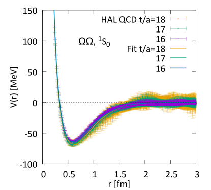
Figure 3: The $\Omega\Omega$ potential in $J=0$ channel from lattice QCD simulations Gongyo:2017fjb . The lattice data are fitted by the form, $V_{\text{fit}}(r)=\sum_{j=1,2,3}c_{j}e^{-(r/d_{j})^{2}}$.

Table 2 shows the low energy scattering parameters and binding energies obtained by solving the Schrödinger equation in the presence of the attraction from the strong interaction and the repulsion from the Coulomb interaction. The already large positive scattering length found in lattice QCD calculations is further driven toward the unitary limit ($a_{0}\gg r_{\rm eff}$) by the Coulomb repulsion. The obtained scattering length exceeds the effective source size in heavy-ion collisions, therefore one can expect the correlation function belongs to the unitary region characterized by $R/a_{0}\sim 0$ in Fig. 1.

Table 2: Scattering length $a_{0}$, effective range $r_{\text{eff}}$, and binding energy of the $\Omega\Omega$ pair with the lattice QCD potential for different $t/a$ and the Coulomb repulsion.

$t/a$	$a_{0}$ [fm]	$r_{\text{eff}}$ [fm]	$E_{B}$ [MeV]
16	65.28	1.29	0.1
17	17.59	1.24	0.54
18	11.69	1.26	1.0

IV.2 Correlation function

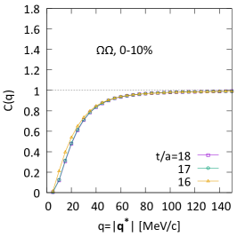
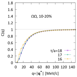
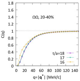
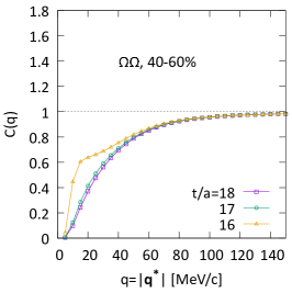
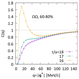
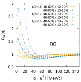
Figure 4: $\Omega\Omega$ correlation function $C(q)$ from central (0-10%) to peripheral (60-80 %) Pb-Pb collisions, as well as the small-to-large ratio $C_{\text{SL}}(q)$.

Assuming that the strong interaction except for the $J=0$ channels is negligible, one may write the wave functions à la Eq. (10) with the Coulomb repulsion and the Fermi statistics (symmetrization for $J=0,2$ and anti-symmetrization for $J=1,3$):

$$\varphi^{J=0}(\bm{q},\bm{r}) =\varphi^{C}_{\text{sym}}(\bm{q},\bm{r})-\varphi^{C}_{0,\text{sym}}(r)+\chi^{C}_{0}(r)$$ (17)

$$\varphi^{J=2}(\bm{q},\bm{r}) =\varphi^{C}_{\text{sym}}(\bm{q},\bm{r}),$$ (18)

$$\varphi^{J=1,3}(\bm{q},\bm{r}) =\varphi^{C}_{\text{asym}}(\bm{q},\bm{r}).$$ (19)

Here $\varphi^{C}_{\text{sym}}(\bm{q},\bm{r})$ and $\varphi^{C}_{\text{asym}}(\bm{q},\bm{r})$ denote the Coulomb wave functions with symmetrization and anti-symmetrization, respectively. Also, $\varphi^{C}_{0,\text{sym}}(r)$ is the S-wave component of $\varphi^{C}_{\text{sym}}(\bm{q},\bm{r})$. The full wave function in the S-wave, $\chi^{C}_{0}(r)$, is obtained by solving the Schrödinger equation with the strong interaction potential $V_{\rm fit}(r)$ in Fig. 3 together with the Coulomb repulsion. In the absence of the Coulomb interaction, these expressions reduce to the case of neutral particles, e.g. $\Lambda\Lambda$ pairs shown in Morita:2014kza . Also note that the wave functions $\phi^{J}$ in Eqs. (17)-(19) contain the higher-partial wave ($L\geq 1$) components. The total probability density is thus given by

$$|\varphi_{\Omega\Omega}(\bm{q},\bm{r})|^{2}=\sum_{J=0}^{3}\frac{2J+1}{16}|\varphi^{J}(\bm{q},\bm{r})|^{2}.$$ (20)

Note that the effect of the strong interaction in $J=0$ is weighted only by 1/16 in the probability.

We calculate the correlation function $C(q)$ in Eq. (5) by combining Eq. (15) and Eq. (20). In the momentum integral, we take vanishing particle rapidities and fix the transverse momentum to the average values obtained from the spectra (Fig. 2). In Fig. 4, $\Omega\Omega$ correlation functions for different centralities are displayed. Note that the system size becomes smaller as the centrality increases. The depletion of $C(q)$ below 1 at small $q$ is due to the Coulomb repulsion and the HBT effect. Also, the latter effect extends to wider region of $q$ for smaller systems. As shown in a schematic analysis given in Fig. 1 (b), the correlation function exhibits stronger FSI effect with decreasing system size. Such a tendency can be seen particularly for the $\Omega\Omega$ potential with $t/a=16$ in Fig. 4, since $a_{0}$ is extremely large.

Shown the bottom-right panel of Fig. 4 is the small-to-large ratio, $C_{\text{SL}}(q)$ between 40-60% (or 60-80%) for small systems and 10-20% for large systems. Due to the cancellation of the Coulomb effect, one now finds notable enhancement of $C_{\text{SL}}(q)$ above 1 for small $q$ due to the strong $\Omega\Omega$ attraction, and the reduction of $C_{\text{SL}}(q)$ below 1 for large $q$ due to the HBT effect.

V $p\Omega$ correlation

Let us now move on to the results for $p\Omega$ correlations. Among $J=1\ (^{5}S_{2})$ and $J=2\ (^{3}S_{1})$ channels which the $p\Omega$ pair can take, the $J=2$ channel is expected to have a shallow bound state as indicated from lattice QCD Iritani:2018sra . Note, however, that the $p\Omega$ pair is not the lowest energy channel in the $S=-3$ dibaryon system: There exist thresholds of the octet-octet states ($\Lambda\Xi$ and $\Sigma\Xi$) at lower energies, which act as absorptive channels for $p\Omega$. The S-wave $J=2$ channel couples to octet-octet states only through the $D$ wave, so that the decay is dynamically suppressed and its effect on the correlation function is considered to be sufficiently small. According to Ref. Sekihara:2018tsb , where the $J=2$ $N\Omega$ interaction is discussed with the meson exchange model including the decay channels, the coupling does not change the weak-binding nature of $p\Omega$. Thus, in the following calculations, we apply the single-channel approximation to the $J=2$ $p\Omega$ correlation function.

In the previous study on $C_{\text{SL}}(q)$ for $p\Omega$ Morita:2016auo , the $J=2$ potential obtained by lattice QCD simulations with heavy quark masses Etminan:2014tya were used. Below, we update the analysis by using the $J=2$ potential for nearly physical quark masses as described below.

V.1 $N\Omega$ interaction from lattice QCD

The $N\Omega$ interaction in $J=2$ channel has been calculated by (2+1)-flavor lattice QCD simulations Iritani:2018sra with the same setup as the $\Omega\Omega$ case discussed in Sec.IV.1. In this case, the Euclidean time interval was chosen to be $t/a=11-14$ to avoid significant statistical errors for large $t$. Resultant potentials with statistical errors are recapitulated in Fig. 5 together with the fitted potential of a Gaussian + (Yukawa)² form. The scattering length and the effective range without the Coulomb interaction are $a_{0}\simeq$ 5.3 fm and $r_{\text{eff}}\simeq$ 1.26 fm, respectively, so that a weakly bound $N\Omega$ appears with the binding energy $E_{B}\sim$ 1.54 MeV.

Table 3 shows the low energy scattering parameters and binding energies obtained by solving the Schrödinger equation in the presence of the attraction from the strong interaction and the extra attraction from the Coulomb interaction. The value of the resultant scattering length is compatible with the expected effective system size in heavy-ion collisions, thus one can expect characteristic depletion of the correlation function and its variation for the system with bound state, against system size as seen from Fig. 1.

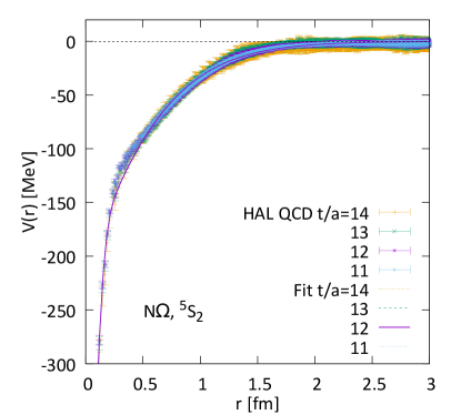
Figure 5: The S-wave $N\Omega$ potential with $J=2$ from lattice QCD simulations Iritani:2018sra . The lattice data are fitted by the form, $V_{\text{fit}}(r)=b_{1}e^{-b_{2}r^{2}}+b_{3}(1-e^{-b_{4}r^{2}})(e^{-m_{\pi}r}/r)^{2}$ with $m_{\pi}$=146 MeV.

Table 3: S-wave scattering length $a_{0}$, effective range $r_{\text{eff}}$, and binding energy of the $p\Omega$ pair with the lattice QCD potential for different $t/a$ and the Coulomb attraction.

$t/a$	$a_{0}$ [fm]	$r_{\text{eff}}$ [fm]	$E_{B}$ [MeV]
11	3.45	1.33	2.15
12	3.38	1.31	2.27
13	3.49	1.31	2.08
14	3.40	1.33	2.24

V.2 Correlation function

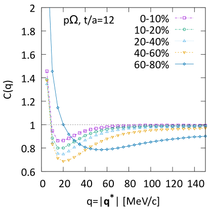
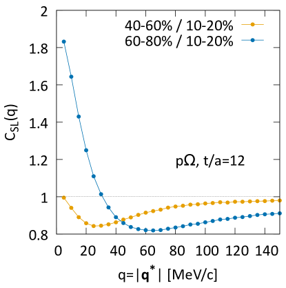
Figure 6: $p\Omega$ correlation function from central (0-10%) to peripheral (60-80 %) Pb-Pb collisions (upper panel), as well as from peripheral to central collisions and the small-to-large ratio (lower panel).

In addition to the $J=2$ channel, the $N\Omega$ system has the $J=1$ channel which is expected to couple strongly with low-lying octet-octet states due to fall apart decay in the S-wave. In the same way as Ref. Morita:2016auo , we consider a limiting case where the $J=1$ $p\Omega$ pairs are perfectly absorbed into low-lying states through the potential $V^{J=1}(r)=-i\theta(r_{0}-r)V_{0}$. The strength $V_{0}$ is taken to be infinity and $r_{0}$ is set to 2 fm where Coulomb interaction dominates over the $J=1$ LQCD potential. Accordingly, the wave function is written as $\varphi^{J}(\bm{q},\bm{r})=\varphi^{C}(\bm{q},\bm{r})-\varphi^{C}_{0}(r)+\chi_{0}^{C}(r)$, where the scattering wave function in the S-wave, $\chi_{0}^{C}(r)$, receives the effects of the interactions.

Then the total probability density reads

$$|\varphi_{p\Omega}(\bm{q},\bm{r})|^{2}=\sum_{J=1}^{2}\frac{2J+1}{8}|\varphi^{J}(\bm{q},\bm{r})|^{2}.$$ (21)

Here the $J=2$ contribution which is of our interest, is weighted by a large factor $5/8$. The number of the low momentum pairs decrease due to the absorption in the $J=1$ channel and the resultant correlation function $C(q)$ tends to decrease but not with significant amount as discussed in in Ref. Morita:2016auo .

Figure 6 shows the $p\Omega$ correlation functions from peripheral to central collisions. Since the $N\Omega$ potential in Fig. 5 is nearly independent of $t/a$, the same holds for $C(q^{*})$ too. Thus we display only results of $t/a=12$. The enhancement of $C(q)$ above 1 for small $q$ is due to the Coulomb attraction whereas the suppression of $C(q)$ below 1 is due to the positive scattering length, or equivalently the existence of $p\Omega$ bound state. The effect of FSI is smallest (largest) in central collisions $(0-10\%)$ (peripheral collisions $(60-80\%)$), so that the region of the suppressed correlation becomes deeper and wider as the system size decreases, in accordance with the moderate value of the scattering length ($a_{0}\simeq 3.4$ fm) in Table 3.

Shown the bottom panel of Fig.6 is the small-to-large ratio, $C_{\text{SL}}(q)$, between 40-60% (or 60-80%) for the small system and 10-20% for the large system. After the cancellation of the Coulomb effect, one now finds notable enhancement of $C_{\text{SL}}(q)$ above 1 at small $q$ and depletion below 1 at $q=(20-80)~{}\mathrm{MeV}$ due to the strong $p\Omega$ attraction accommodating a bound state. In response to the theoretical proposal in Morita:2016auo , the STAR collaboration at RHIC has reported a first measurement of $p\Omega$ correlation in Au+Au collisions STAR:2018uho . Although the statistics of the data are not sufficient to draw a definitive conclusion, the measured $C(q)$ and $C_{\text{SL}}(q)$ show similar tendency with Fig.6 in the present paper.

VI Summary and Concluding remarks

We have studied the two-particle momentum correlations for $\Omega\Omega$ and $p\Omega$ in relativistic heavy-ion collisions. The correlation functions are calculated by using an expanding source model combined with the latest lattice QCD potentials which predict shallow bound states with relatively large positive scattering lengths in the $J=0$ $\Omega\Omega$ and the $J=2$ $N\Omega$.

At the LHC energies, the correlation function $C(q)$ for $\Omega\Omega$ in Pb-Pb collisions exhibits an enhancement due to large scattering length ($a_{0}>$ 10 fm) over the Coulomb repulsion and the HBT effect, especially in the peripheral events. This characteristic feature can be best visible and quantified as an enhancement of the small-to-large ratio $C_{\text{SL}}(q)$ at $q<40$ MeV/c.

On the other hand, the characteristic feature of the correlation function $C(q)$ of $p\Omega$ is its depletion below 1 at $q=20-40$ MeV due to the moderately large value of the positive scattering length $a_{0}\simeq 3.4$ fm. Properly chosen small-to-large ratio $C_{\text{SL}}(q^{*})$ also exhibits this behavior.

Measuring the $\Omega\Omega$ in heavy-ion collisions is a challenge even with the high luminosity upgrade of LHC due to its small production rate as well as the correlation measurement at small $q\ (<50$ MeV). Therefore, not only the luminosity upgrade but also the improvements of measurement techniques would be necessary.

In response to our theoretical proposal in Morita:2016auo , the STAR collaboration at RHIC has reported a first measurement of $p\Omega$ correlation in Au+Au collisions STAR:2018uho . Although the statistics of the data are not sufficient to draw a definitive conclusion, the measured $C(q)$ and $C_{\text{SL}}(q)$ show similar tendency with Fig.6 in the present paper. Also the ALICE Collaboration at LHC has started the $p\Omega$ measurements with $pp$ and $p$-Pb collisions  ALICE:pOmega . Extracting the $p\Omega$ interaction from a combined theoretical analysis of the $pp$, $pA$ and $AA$ collisions with proper uncertainty quantification would be an interesting future problem. (See Appendix A for an exploratory study along such direction.)

In order to draw definite conclusion on the existence of the $\Omega\Omega$ and $N\Omega$ dibaryon bound states from the future and existing correlation function data, we need further works to be done. First, it is desired to obtain not only the $J=0$ $\Omega\Omega$ potential and $J=1$ $N\Omega$ potential but also the $J=1,2$ and $3$ $\Omega\Omega$ potentials and the $J=1$ $N\Omega$ potential. Second, the coupled channel effects need to be clarified. As discussed in the Appendix A, the $J=1$ contribution causes visible uncertainties in the $p\Omega$ correlation function. While the coupling effects to octet-octet channels with $J=1$ in the $p\Omega$ correlation function have been assumed to be described by the absorption, the coupled channel formula Haidenbauer:2018jvl shows that creation processes such as $\Lambda\Xi\to p\Omega$ also contribute to the correlation function of $p\Omega$. Then we need to evaluate the transition potentials and the source function of $\Lambda$ and $\Sigma$.

Appendix A System size dependence of $C(q)$ for $p\Omega$ with uncertainty quantification

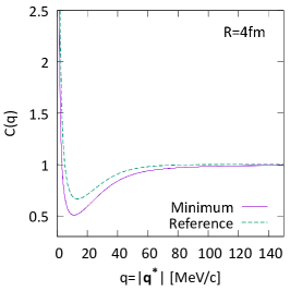
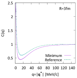
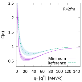
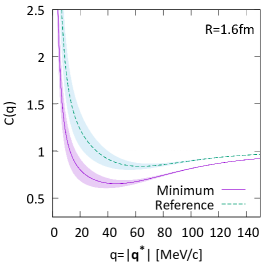
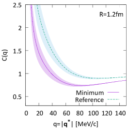
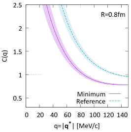
Figure 7: $p\Omega$ correlation function calculated with the static Gaussian source function employing the $t/a=12$ potential. The purple solid line denotes the result with $\chi_{0}^{C,J=1}=0$, and blue dashed line denotes the result with the assumption of $\chi_{0}^{C,J=1}=\chi_{0}^{C,J=2}$. Gaussian source size is chosen to be in the range $R=0.8$ - $4\ \mathrm{fm}$. The error of each correlation estimated with the Jackknife method is shown by the colored shadow.

In the light of feasibility of measuring $p\Omega$ correlation in $pp$, $pA$ and $AA$ collisions, it is desirable to get a feel for theoretical uncertainties in evaluating the momentum correlations. In the following, we focus on the uncertainties originating from the $J=2$ $p\Omega$ potential from lattice QCD and from the treatment of the unknown $J=1$ $p\Omega$ potential. To make the discussion transparent, we consider a simplified static and spherically symmetric Gaussian source function $S(r)=(4\pi R^{2})^{-3/2}\exp(-r^{2}/4R^{2})$ with the source size ranging from 0.8 to 4 fm.

For uncertainties arising from the insufficient information on the $J=1$ potential, we evaluate “minimum” and “reference” contributions from the $J=1$ channel. The “minimum” is obtained by assuming $\chi^{C,J=1}_{0}(r)=0$, i.e. complete absorption of the wave function in all range of $r$. This leads to the minimum value of $C(q)$ as seen in Eq. (11). The “reference” is obtained by assuming $\chi^{C,J=1}_{0}(r)=\chi^{C,J=2}_{0}(r)$, i.e. the same attraction between $J=1$ and $J=2$ without absorption. The statistical uncertainty for each case is estimated by the statistical error of the $J=2$ $N\Omega$ potential at $t/a=12$ by the Jackknife method in the similar way as  Iritani:2018sra .

The results of $C(q)$ for different values of $R$ are shown in Fig. 7. The shaded areas represent the statistical errors obtained from the Jackknife analysis. For $R\leq 2$ fm, the “minimum” and “reference” correlation functions exhibit sizable differences with larger statistical uncertainty. This is because the condition for the unitary region shown in Fig. 1 begins to hold with $a_{0}\simeq 3.4$ fm in Table 3), so that the correlation function becomes more sensitive to the uncertainty of the potential as well as the treatment of the $J=1$ channel.

Within the above uncertainty estimate, we can safely conclude that the correlation function can be strongly suppressed at $q<40~{}\mathrm{MeV}$ for systems with $2\text{ fm}\lesssim R\lesssim 4$ fm. We also find that the suppressed region of $C(q)$ moves toward the lower $q$ direction with increasing source size. This behavior is consistent with the trend found in the data from Au+Au collisions by the STAR Collaboration at RHIC STAR:2018uho . By comparison, strong enhancement at small momenta would be observed for small systems with $R\simeq 1~{}\mathrm{fm}$ as found in the preliminary data by the ALICE Collaboration at LHC ALICE:pOmega .

Appendix B Comparison of $N\Omega$ potentials

We here compare the $J=2$ $N\Omega$ potential used in this work and those used in Morita:2016auo . The former is obtained from LQCD simulations with nearly physical quark masses ($m_{\pi}=146~{}\mathrm{MeV}$ and $m_{K}=525~{}\mathrm{MeV}$)  Iritani:2018sra , while the latter is those with heavier quark masses ($m_{\pi}=875~{}\mathrm{MeV}$ and $m_{K}=916~{}\mathrm{MeV}$) Etminan:2014tya . In Fig. 8, we show the $J=2$ $N\Omega$ potential with nearly physical quark masses at $t/a=12$ (solid curve), and the potentials given in Morita:2016auo , $V_{\mathrm{I}}$ (dashed), $V_{\mathrm{II}}$ (dotted) and $V_{\mathrm{III}}$ (dash-dotted). The potential $V_{\mathrm{II}}$ is the best fit of the lattice data with heavier quark masses with a form $V_{\text{fit}}(r)=b_{1}e^{-b_{2}r^{2}}+b_{3}(1-e^{-b_{4}r^{2}})(e^{-b_{5}r}/r)^{2}$. $V_{\mathrm{I}}$ and $V_{\mathrm{III}}$ are two typical examples with weaker and stronger attractions, respectively. These potentials together with the Coulomb potential give no bound state for $V_{\mathrm{I}}$, a shallow bound state $E_{B}\simeq 0.63~{}\mathrm{MeV}$ for $V_{\mathrm{II}}$,, and a deep bound state $E_{B}\simeq 26.9~{}\mathrm{MeV}$ for $V_{\mathrm{III}}$.

We find that the potential with nearly physical quark masses is between $V_{\mathrm{II}}$ and $V_{\mathrm{III}}$; the attraction becomes stronger with smaller quark masses, but not as attractive as $V_{\mathrm{III}}$. Consequently, the $p\Omega$ correlation function shown in this work is also between those with $V_{\mathrm{II}}$ and $V_{\mathrm{III}}$ shown in Morita:2016auo .

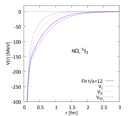
Figure 8: Comparison of the S-wave $N\Omega$ potentials with $J=2$ in Refs. Iritani:2018sra and Morita:2016auo . The solid curve show the $N\Omega$ potential with nearly physical quark masses Iritani:2018sra at $t/a=12$. The dashed, dotted, and dash-dotted curves show the $J=2$ $N\Omega$ potentials, $V_{\mathrm{I}}$, $V_{\mathrm{II}}$ and $V_{\mathrm{III}}$, given in Morita:2016auo .

References

- (1) A. Gal, Acta Phys. Polon. B 47, 471 (2016).
- (2) H. Clement, Prog. Part. Nucl. Phys. 93, 195 (2017).
- (3) H. C. Urey, F. G. Brickwedde, and G. M. Murphy, Phys. Rev. 39, 164 (1932).
- (4) W. Rarita and J. Schwinger, Phys. Rev. 59, 436 (1941).
- (5) R. L. Jaffe, Phys. Rev. Lett. 38, 195 (1977) [Erratum: Phys. Rev. Lett. 38, 617 (1977)].
- (6) T. Goldman, K. Maltman, G. J. Stephenson, Jr., K. E. Schmidt and F. Wang, Phys. Rev. Lett. 59, 627 (1987).
- (7) M. Oka, Phys. Rev. D 38, 298 (1988).
- (8) V. B. Kopeliovich, B. Schwesinger and B. E. Stern, Phys. Lett. B 242, 145 (1990).
- (9) N. Ishii, S. Aoki and T. Hatsuda, Phys. Rev. Lett. 99, 022001 (2007); S. Aoki, T. Hatsuda and N. Ishii, Prog. Theor. Phys. 123, 89 (2010).
- (10) N. Ishii, S. Aoki, T. Doi, T. Hatsuda, Y. Ikeda, T. Inoue, K. Murano, H. Nemura and K. Sasaki (HAL QCD Collaboration), Phys. Lett. B 712, 437 (2012).
- (11) T. Doi and M. G. Endres, Comput. Phys. Commun. 184, 117 (2013).
- (12) S. Gongyo et al. (HAL QCD Collaboration), Phys. Rev. Lett. 120, 212001 (2018).
- (13) T. Iritani et al. (HAL QCD Collaboration), Phys. Lett. B 792, 284 (2019).
- (14) S. Cho et al. (ExHIC Collaboration), Phys. Rev. Lett. 106, 212001 (2011); Phys. Rev. C 84, 064910 (2011).
- (15) S. Cho et al. (ExHIC Collaboration), Prog. Part. Nucl. Phys. 95, 279 (2017).
- (16) K. Morita, T. Furumoto and A. Ohnishi, Phys. Rev. C 91, 024916 (2015).
- (17) K. Morita, A. Ohnishi, F. Etminan and T. Hatsuda, Phys. Rev. C 94, 031901(R) (2016).
- (18) A. Ohnishi, K. Morita, K. Miyahara and T. Hyodo, Nucl. Phys. A 954, 294 (2016).
- (19) T. Hatsuda, K. Morita, A. Ohnishi and K. Sasaki, Nucl. Phys. A 967, 856 (2017).
- (20) J. Adam et al. (STAR Collaboration), Phys. Lett. B 790, 490 (2019).
- (21) M. A. Lisa, S. Pratt, R. Soltz and U. Wiedemann, Ann. Rev. Nucl. Part. Sci. 55, 357 (2005).
- (22) D. Anchishkin, U. W. Heinz and P. Renk, Phys. Rev. C 57, 1428 (1998); R. Lednicky, Phys. Part. Nucl. 40, 307 (2009).
- (23) T. Csorgo and B. Lorstad, Phys. Rev. C 54, 1390 (1996); S. Chapman, P. Scotto and U. W. Heinz, Acta Phys. Hung. A 1, 1 (1995).
- (24) S. Pratt, Phys. Rev. Lett. 102, 232301 (2009).
- (25) R. Lednicky and V. L. Lyuboshits, Sov. J. Nucl. Phys. 35, 770 (1982) [Yad. Fiz. 35, 1316 (1981)].
- (26) J. Haidenbauer, Nucl. Phys. A 981, 1 (2019).
- (27) B. B. Abelev et al. (ALICE Collaboration), Phys. Lett. B 728, 216 (2014) [Erratum: Phys. Lett. B 734, 409 (2014)].
- (28) B. Abelev et al. (ALICE Collaboration), Phys. Rev. C 88, 044910 (2013).
- (29) A. Andronic, P. Braun-Munzinger, K. Redlich and J. Stachel, Nature 561. 7723, 321 (2018).
- (30) X. Zhu, F. Meng, H. Song and Y. X. Liu, Phys. Rev. C 91, 034904 (2015).
- (31) A. N. Makhlin and Y. M. Sinyukov, Z. Phys. C 39, 69 (1988).
- (32) A. Andronic, P. Braun-Munzinger, B. Friman, P. M. Lo, K. Redlich and J. Stachel, Phys. Lett. B 792, 304 (2019).
- (33) J. Adam et al. (ALICE Collaboration), Phys. Rev. C 92, 054908 (2015).
- (34) T. Sekihara, Y. Kamiya and T. Hyodo, Phys. Rev. C 98, 015205 (2018).
- (35) F. Etminan et al. (HAL QCD Collaboration), Nucl. Phys. A 928, 89 (2014).
- (36) O. Vázquez Doce et al. (ALICE Collaboration), ”Femtoscopic studies on proton- and proton- correlations”, (2019), Poster presentation at SQM 2019.