Volterra-series approach to stochastic nonlinear dynamics: linear response of the Van der Pol oscillator driven by white noise

Abstract

The Van der Pol equation is a paradigmatic model of relaxation oscillations. This remarkable nonlinear phenomenon of self-sustained oscillatory motion underlies important rhythmic processes in nature and electrical engineering. Relaxation oscillations in a real system are usually coupled to environmental noise, which further enriches their dynamics, but makes theoretical analysis of such systems and determination of the equation’s parameter values a difficult task. In a companion paper we have proposed an analytic approach to a similar problem for another classical nonlinear model, the bistable Duffing oscillator. Here we extend our techniques to the case of the Van der Pol equation driven by white noise. We analyze the statistics of solutions and propose a method to estimate parameter values from the oscillator’s time series. We use experimental data of active oscillations in a biological system to demonstrate how our method applies to real observations and how it can be generalized for more complex models.

I Introduction

Balthazar van der Pol introduced the concept of relaxation oscillations together with his eponymous equation for a simplified dynamics of a triode electric circuit van der Pol (1926); Ginoux and Letellier (2012). Regarded as a power-series approximation for a more general class of Lienard systems (Strogatz, 2014, Sec. 7.4 and 7.5), this model became a paradigm of self-sustained oscillatory motion Ginoux and Letellier (2012). Besides its applications in engineering, the Van der Pol equation and its generalizations are used to describe various rhythmic processes in biology Beta and Kruse (2017); Oates et al. (2012); Buzsáki and Draguhn (2004); Nomura et al. (1993); Rompala et al. (2007); Duifhuis et al. (1986); Talmadge et al. (1990); van Dijk and Wit (1990); van der Pol (1928, 1940); Mirollo and Strogatz (1990); Cherevko et al. (2016, 2017); FitzHugh (1961); Nagumo et al. (1962); Izhikevich and FitzHugh (2006); Alonso et al. (2014); Mindlin (2017).

Self-sustained oscillations are ubiquitous in living systems on different length and time scales. Examples include intracellular oscillations of molecular concentrations Beta and Kruse (2017), pattern formation and dynamics of tissues Oates et al. (2012), neuronal activity Buzsáki and Draguhn (2004); Nomura et al. (1993), circadian clocks Rompala et al. (2007), otoacoustic emissions from the ear Duifhuis et al. (1986); Talmadge et al. (1990); van Dijk and Wit (1990), the beating of a heart van der Pol (1928, 1940), the synchronized flashing of fireflies Mirollo and Strogatz (1990), and hemodynamics Cherevko et al. (2016, 2017). Much theoretical work has been devoted to developing mathematical description for such systems Roenneberg et al. (2008). Often the existing models rely on parameters that are difficult to determine from experimental data. The mathematical description is then limited to qualitative or conceptual studies.

To facilitate quantitative research we develop analytical techniques for self-sustained oscillations of the Van der Pol type with a moderate level of noise. In particular, we derive approximate expressions for the linear response of the Van der Pol oscillator. In our approach the nonlinear problem of self-sustained oscillations can thus be mapped onto an effective linear model that reproduces the main features of the original system.

Furthermore, we propose a method to estimate parameter values of the Van der Pol equation directly from time series, as typically observed in experiments. By fitting empirical observations to the analytical expressions that we derive, it is straightforward to determine the underlying model. We demonstrate and validate this approach with stochastic simulations (Sec. III) and experimental data of active oscillations from a bullfrog’s mechanoreceptive cells in the inner ear (Sec. IV).

A general form of the Van der Pol equation that we consider in this paper extends the harmonic oscillator by introducing a nonlinear dissipative term in the equation

$$\ddot{x}+a\dot{x}+bx+c\dot{x}x^{2}=f$$ (1)

for an unknown function of time $x(t)$ and an external force $f(t)$; the constants $a$, $b$, and $c$ are, respectively, the friction coefficient, the stiffness, and the Van der Pol damping parameter. Because the above equation is of second order in time, the phase of this system is specified by two degrees of freedom $(x,\dot{x})$.

The self-sustained oscillations of the Van der Pol equation correspond to its limit-cycle solution. In the absence of the external force $f(t)$, all trajectories of this system relax to a periodic orbit in the phase space. Self-sustained oscillations exist if the friction constant in Eq. (1) is negative ($a<0$). The Van der Pol system is stable when the parameters $b$ and $c$ are both positive. The amplitude of the limit cycle, which encircles an unstable equilibrium point in the phase space, shrinks to zero when $a=0$ and disappears for $a>0$. Therefore the Van der Pol oscillator with $a\geq 0$ behaves as a monostable system. This dynamical regime is not studied in the present paper and should be treated by a different approach (Belousov et al., 2019, Appendix A).

Environmental noise, which intertwines with relaxation oscillations of real systems, is often modeled by a stochastic force $f(t)=A\dot{w}(t)$, with a constant amplitude $A>0$ and Gaussian white noise $\dot{w}(t)$ of zero mean and unit intensity. One must usually resort to complex measures to determine the model’s parameter values for this class of stochastic nonlinear problems Alonso et al. (2014); Mindlin (2017); Cherevko et al. (2016, 2017).

Previously we demonstrated that time series of a second-order dynamical system—the stochastic Duffing oscillator—contains enough information to infer the parameter values of the underlying nonlinear model Belousov et al. (2019). Here we extend our analysis to the case of Van der Pol relaxation oscillations driven by white noise. After deriving analytical expressions for approximate solutions and time-series statistics of Eq. (1), we use these formulas to devise a parametric method of inference.

Our approach is based on the functional series of Volterra Schetzen (2006); Rugh (1981), which we expand up to the linear-response term. The analytical results and the inference method that we propose are therefore applicable to relatively small noise amplitudes $A$; more details on the system’s physical scales are given in Sec. III. Even in the absence of external driving, the statistical properties of the relaxation oscillations are far from trivial. This feature of the Van der Pol equation renders the time-series analysis more difficult than in the case of the Duffing oscillator Belousov et al. (2019). Because we must also approximate the limit-cycle solution of Eq. (1), for which no closed-form expression is known, our development is restricted to moderate regimes of driving noise and nonlinear behavior.

II Theory

II.1 Linear response of the Van der Pol oscillator

A Volterra series is a polynomial functional expansion of the form

$$x(t|f)=x_{0}(t)+\int_{0}^{t}dt_{1}\,g_{1}(t-t_{1})f(t_{1})\\ +\iint_{0}^{t}dt_{1}dt_{2}\,g_{2}(t-t_{1},t-t_{2})f(t_{1})f(t_{2})+...\\$$ (2)

in which $g_{1}(t)$ and $g_{2}(t)$ are the Volterra kernels of the linear and quadratic terms in the argument function $f(t)$. Provided that the above series exists, a truncated expansion (2) approximates solutions of Eq. (1) driven by a small external force:

$$x(t)\simeq x_{0}(t)+\int_{0}^{t}dt_{1}\,g_{1}(t-t_{1})f(t_{1})\\ =x_{0}(t)+\gamma_{1}(t),$$ (3)

in which we neglect terms of the second and higher orders in $f(t)$. The functions $x_{0}(t)$ and $\gamma_{1}(t)$ can be found by using the variational approach (Belousov et al., 2019; Rugh, 1981, Sec. 3.4), which yields a set of equations

$$\ddot{x}_{0}+a\dot{x}_{0}+bx_{0}+c\dot{x}_{0}x_{0}^{2} = 0,$$ (4)

$$\ddot{\gamma}_{1}+(a+cx_{0}^{2})\dot{\gamma}_{1}+(b+2c\dot{x}_{0}x_{0})\gamma_{1} = f,$$

$$\cdots$$

Equation (4), which uniquely defines $x_{0}(t)$ for a given initial condition $\big{(}x(0),\dot{x}(0)\big{)}$, is equivalent to the autonomous Van der Pol problem—Eq. (1) with $f\equiv 0$. The linear Eq. (II.1), which determines the first-order Volterra term $\gamma_{1}(t)$, in general contains time-dependent coefficients.

Because the Volterra series generalizes the Taylor-Maclaurin expansion of functions in calculus (Rugh, 1981, Sec. 1.5), Eq. (2) may be restricted by a radius of convergence or may even fail to exist for some choices of $x_{0}(t)$. The equilibrium point $x_{0}(t)\equiv 0$, which is a convenient choice for the monostable case of Eq. (1), is unstable in the regime of relaxation oscillations and yields a divergent kernel $g_{1}(t)$. With $x_{0}(t)\equiv 0$ we therefore cannot construct an approximate representation (3) that is valid for long time scales Belousov et al. (2019).

For the above reason we use the Volterra series expansion about $x_{0}(t)$ that represents the stable limit-cycle solution of Eq. (4). Because a closed-form expression of this solution is unknown, as its approximation one may adopt a truncated Fourier expansion $x_{0}(t)\approx\xi(t)$ that can be obtained by various methods (Jordan and Smith, 2007, Sections 4.4 and 5.9). Substituting $\xi(t)$ for $x_{0}(t)$ in Eq. (II.1) we obtain a linear problem

$$\ddot{\gamma}_{1}+a_{\xi}\dot{\gamma}_{1}+b_{\xi}\gamma_{1}=f,$$ (6)

with time-dependent periodic coefficients

$$a_{\xi}(t)=a+c\xi(t)^{2},$$ (7)

$$b_{\xi}(t)=b+2c\dot{\xi}(t)\xi(t).$$ (8)

Note that the time-dependent friction $a_{\xi}(t)$ and stiffness $b_{\xi}(t)$ oscillate around positive average values that ensure the stability of Eq. (6). These coefficients are statistically independent from the driving white-noise force $f(t)$ at all times. On average the response of the linear stochastic Eq. (6) can be therefore described by effective friction and stiffness constants. To implement this simplification for the quasiperiodic term $\gamma_{1}(t)$, in the spirit of time-averaging methods (Chapter 4 in Jordan and Smith, 2007; Grimshaw, 2017, Sec. 9.2) we replace the periodic coefficients in Eq. (6) by their mean values

$$\langle a_{\xi}(t)\rangle=\int_{0}^{2\pi/\sqrt{b}}\frac{\sqrt{b}dt}{2\pi}a_{\xi}(t),$$ (9)

$$\langle b_{\xi}(t)\rangle=\int_{0}^{2\pi/\sqrt{b}}\frac{\sqrt{b}dt}{2\pi}b_{\xi}(t),$$ (10)

in which the ensemble average of a periodic function is related to the time average over one period $2\pi/\sqrt{b}$. In this approximation Eq. (6) describes a harmonic oscillator $\tilde{\gamma}(t)\approx\gamma_{1}(t)$:

$$\ddot{\tilde{\gamma}}-\langle a_{\xi}\rangle\dot{\tilde{\gamma}}+\langle b_{\xi}\rangle\tilde{\gamma}=f$$ (11)

with the linear response function

$$g_{\xi}(t)=\Omega^{-1}\operatorname{\mathrm{e}}^{-\frac{\langle a_{\xi}\rangle t}{2}}\sin(\Omega t)\approx g_{1}(t),$$ (12)

in which $\Omega=\sqrt{\langle b_{\xi}\rangle-\langle a_{\xi}\rangle^{2}/4}$. If $\Omega^{2}<0$ one should use $\sqrt{\langle a_{\xi}\rangle^{2}/4-\langle b_{\xi}\rangle}$ instead of $\Omega$ and replace the trigonometric sine in Eq. (12) by the hyperbolic one (Belousov and Cohen, 2016; Chandrasekhar, 1943, Sec. II-3).

The approximate solution of the stochastic Van der Pol equation (1) is thus expressed by a sum of two independent contributions $\xi(t)$ and $\tilde{\gamma}(t)$

$$x(t)\approx x_{\xi}(t)=\xi(t)+\tilde{\gamma}(t)=\xi(t)+\int_{0}^{t}dsg_{\xi}(t-s)f(s).$$ (13)

The linear-response term $\tilde{\gamma}(t)$ in the above equation has a Gaussian probability density, with a zero mean $\langle\tilde{\gamma}\rangle=0$ and an autocovariance function Belousov and Cohen (2016)

$$\langle\tilde{\gamma}(0)\tilde{\gamma}(t)\rangle=\frac{A^{2}}{2\langle a_{\xi}\rangle\langle b_{\xi}\rangle}\exp\left(-\frac{\langle a_{\xi}\rangle t}{2}\right)\\ \times\left[\cos(\Omega t)+\frac{\langle a_{\xi}\rangle}{2\Omega}\sin(\Omega t)\right].$$ (14)

In Appendix A we derive two levels of approximations for the autonomous term $x_{0}(t)$, viz. $\xi_{0}(t)$ and $\xi_{1}(t)$ [Eqs. (29) and (30)]. A comparison of the noisy Van der Pol oscillator $x(t)$ with the limit-cycle solution $x_{0}(t)$ and a single-mode Fourier expansion $\xi_{0}(t)$ is shown in Fig. 1. The trajectory $\xi_{0}(t)$ approximates well the period of oscillations and the overall trend of the time series $x(t)$. For moderate values of the noise amplitude $A$ and the parameter $\mu=-a/\sqrt{b}$, which controls the nonlinear character of oscillations (Sec. III), the error of the single-mode approximation $x_{0}(t)\approx\xi_{0}(t)$ is less than or comparable to the uncertainty of the trajectory $x(t)$.

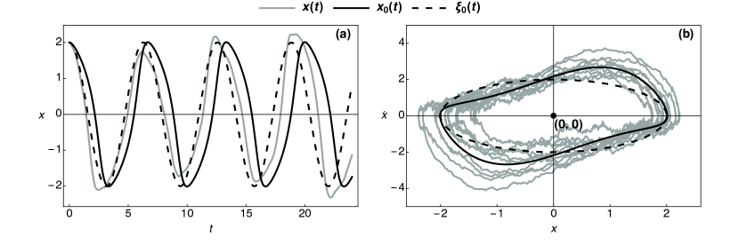
Figure 1: Comparison of the noisy Van der Pol oscillator $x(t)$ with the limit-cycle solution $x_{0}(t)$ and an approximate expression $\xi_{0}(t)$. The system parameters are $\mu=1$ and $A=0.6$ in the reduced units (Sec. III), whereas the initial conditions are set to $(x,\,\dot{x})=(\alpha,\,0)$. Panel (a): phases of the noisy oscillations’ peaks fluctuate around the maxima of $x_{0}(t)$; the theoretical expression $\xi_{0}(t)$ [Eq. (29)] captures the overall trend of the time series $x(t)$. Panel (b): comparison of the phase-space orbits $\big{(}x(t),\,\dot{x}(t)\big{)}$, $\big{(}x_{0}(t),\,\dot{x}_{0}(t)\big{)}$, and $\big{(}\xi_{0}(t),\,\dot{\xi_{0}}(t)\big{)}$; the deviations of the Van der Pol limit cycle $x_{0}(t)$ from the single-mode harmonic approximation $\xi_{0}(t)$ is less than or comparable to the uncertainty of the trajectory $x(t)$.

The approximate solution $x_{\xi}(t)$ is limited to small noise amplitudes not only due to the truncation error in Eq. (2). The external stochastic force induces variations of the oscillator’s phase $\phi=\sqrt{b}t_{0}$ in the periodic term $\xi(t)\to\xi(t-t_{0})$. This effect of noise is especially large when the system’s trajectory is driven close to the point $(x,\dot{x})=(0,0)$. Crossing this point may cause a shift through a phase angle as large as $\phi=\pi$, which requires in general a large force $f(t)$.

At moderate noise amplitudes the above phase variations average to zero [Fig. 1(a)]. Consequently, the time-invariant statistics of $x_{\xi}(t)$, which is analyzed in Appendix B, agrees with that of the noisy Van der Pol oscillator $x(t)$. Their time autocorrelation functions coincide, however, only at small time $t$ (Appendix B, Fig. 6).

Finally, we remark that the approximate solution Eq. (13) can be generated by a forced harmonic oscillator. Such a representation provides a way to emulate self-sustained oscillations of the Van der Pol type by using a linear system with a periodic driving, which is much simpler to analyze quantitatively. This idea is demonstrated in Sec. IV.

II.2 Parametric inference

Equation (13), together with the analysis presented in Appendices A and B, encompasses a simple inference technique that can be used to extract the parameter values $a$, $b$, $c$, and $A$ for Eq. (1) directly from time series of the Van der Pol oscillator. The procedure consists of two curve-fitting steps. First we determine the parameters $a$ and $b$ from the empirical autocorrelation function of the time series $x(t)$. Then we extract the parameters $c$ and $A$ from the oscillatory trend of the trajectory and the variance $\langle x^{2}\rangle$, respectively.

To fit the empirical autocorrelation function $\chi(t)$ we adopt a theoretical Eq. (38) from Appendix B in the form

$$\chi(t)\simeq\frac{\lambda_{1}^{2}\cos(\omega t)}{(\lambda_{1}^{2}+\lambda_{2}^{2})(1+5\mu^{2}/32)}\left\{1+\frac{\mu^{2}}{32}[4+\cos(2\omega t)]\right\}+\frac{\lambda_{2}^{2}}{\lambda_{1}^{2}+\lambda_{2}^{2}}\operatorname{\mathrm{e}}^{-\left(1+\frac{5\mu^{2}}{16}\right)\frac{\mu\omega t}{2}}\left\{\cos\left[\frac{\omega t}{2}\sqrt{4-\left(1+\frac{5\mu^{2}}{16}\right)^{2}\mu^{2}}\right]\right.\\ \left.+\mu\left(1+\frac{5\mu^{2}}{16}\right)\left[4-\left(1+\frac{5\mu^{2}}{16}\right)^{2}\mu^{2}\right]^{-1/2}\sin\left[\sqrt{4-\left(1+\frac{5\mu^{2}}{16}\right)^{2}\mu^{2}}\frac{\omega t}{2}\right]\right\}.$$ (15)

Because the fitting constants $\lambda_{1}^{2}\propto\langle\xi^{2}\rangle$ and $\lambda_{2}^{2}\propto\langle\tilde{\gamma}^{2}\rangle$ are determined up to an arbitrary factor, they are treated as nuisance parameters in the above expression.

Equation (15) approaches its first zero as $t\to\tau\approx\pi/(2\sqrt{b})$, approximately a quarter period of the trigonometric factors in this theoretical expression. We may then apply the criterion of Lagarkov and Sergeev Lagar’kov and Sergeev (1978); Belousov and Cohen (2016) to select the interval $0\leq t\leq\tau$ over which Eq. (15) is expected to be accurate, that is, the initial decay of the empirical time autocorrelations (Appendix B). Because this theoretical expression is very flexible, the initial guess of the fitting constants must be chosen with care. For the best performance we suggest using $\mu\lesssim 1$, $\omega\sim\pi/(2\tau)$, $\lambda_{1,2}\sim\sqrt{\langle x^{2}\rangle/2}$. The parameters of interest $a=-\mu\omega$ and $b=\omega^{2}$ are then found from the optimized values of the constants $\mu$ and $\omega$. To estimate the uncertainties of $\mu$ and $\omega$ we repeat the fitting procedure over few slightly longer intervals of duration $\tau<t<2\tau$.

In the next step of the inference method we estimate the amplitude of the Van der Pol limit-cycle oscillations. Equation (13) decomposes the trajectory $x(t)$ into a sum of the oscillatory term $\xi_{0}(t)\approx\xi(t)$, that determines the average trend, and the Gaussian random-error term $\tilde{\gamma}(t)$. As discussed in Sec. II.1, the limit-cycle solution $x_{0}(t)$ does not account for the slowly fluctuating phase of the noisy Van der Pol oscillations. As in the case of the stochastic Duffing oscillator Belousov et al. (2019), we circumvent this issue by applying Eq. (13) locally: the time series of $x(t)$ can be split into pieces $x_{+}(t)$ and $x_{-}(t)$ for, respectively, $x(t)>0$ and $x(t)<0$. The duration of each component corresponds approximately to a half period $\pi/\sqrt{b}$ of $\xi(t)$. Assuming that the phase shift is constant over one period of oscillations, we then fit these pieces of the whole trajectory to the following formula:

$$x_{0}(t)\simeq\xi_{0}(t-t_{0})=\alpha_{c}\cos(\sqrt{b}t)+\alpha_{s}\sin(\sqrt{b}t),$$ (16)

in which

$$\alpha_{c}=\alpha\cos(\sqrt{b}t_{0}),\quad\alpha_{s}=\alpha\sin(\sqrt{b}t_{0})$$ (17)

cf. Eq. (29) in Appendix A. Note that the constant $b$ in Eq. (16) is fixed to the value estimated from the first step of the method. We also ensure that fitted trajectories have a minimal duration of $\pi b^{-1/2}/2$.

From the optimized values of the fitting constants $\alpha_{c}$ and $\alpha_{s}$, we obtain the amplitude of limit-cycle oscillations and the remaining parameters of interest:

$$\alpha=\sqrt{\alpha_{c}^{2}+\alpha_{s}^{2}},\;c=-\frac{4a}{\alpha^{2}},\;A=\sqrt{ab(2\langle x^{2}\rangle-\alpha^{2})},$$ (18)

in which $\langle x^{2}\rangle$ is the sample variance of the empirical time series $x(t)$. The parameter $\alpha$ and its uncertainty are determined by averaging over all trajectory pieces $x_{\pm}(t)$.

The numerical error of fitting the approximate Eq. (16) to the trajectory pieces $x_{\pm}(t)$ eventually may exceed the uncertainty of the driving noise $f(t)$. Therefore, when the autonomous term $\xi_{0}(t)\propto\alpha$ dominates the statistical variability of the data, a small noise amplitude $A\to 0$ cannot be inferred accurately. Unfortunately a more elaborate approximation $\xi(t)\simeq\xi_{1}(t-t_{0})$ [Appendix A, Eq. (30)] cannot address this issue. As Fourier series are able to match almost any curve arbitrarily close with a sufficient number of terms, the truncated higher-order expansion $\xi_{1}(t)$ overfits noisy trajectories of $x(t)$.

III Application to simulated data

In the system of units reduced by a time constant $b^{-1/2}$ and a length constant $\sqrt{-a/c}$, Eq. (1) takes a canonical form (Strogatz, 2014, Sec. 7.4 and 7.5)

$$\ddot{x}-\mu(1-x^{2})\dot{x}+x=\frac{A}{b\sqrt{-a/c}}\dot{w},$$ (19)

in which the parameter $\mu=-a/\sqrt{b}$ controls the nonlinear character of the dynamics. The greater its value, the larger is the amplitude of the relaxation oscillations. This parameter represents the ratio of two time scales $b^{-1/2}$ and $-a=\mu b^{-1/2}$.

Two control parameters of Eq. (19) that are not fixed in the system of reduced units are $\mu$ and $A$. Without external driving the Van der Pol oscillator, which orbits around the origin of the phase space with the amplitude $\alpha=2\sqrt{-a/c}$ in the harmonic potential $U(x)=bx^{2}/2$ [Fig. 1], has an energy scale

$$U(\alpha)=b\alpha^{2}/2=2\mu b^{3/2}/c.$$

The energy scale of the external force $f(t)=A\dot{w}(t)$ is $A^{2}/\sqrt{b}$. One might therefore expect the small-force expansion Eq. (3) to hold for

$$A<\sqrt{\sqrt{b}U(\alpha)}=b\sqrt{2\mu/c},$$

which relates the two control parameters of Eq. (19) $A$ and $\mu$.

To test the theory presented in the previous section, we simulated Eq. (1) for selected values of noise amplitudes $A$. The computational details are summarized in Appendix C. As a typical value we choose to fix the parameter $\mu=1$. For increasingly large values of $\mu$ Eq. (16) becomes progressively less accurate. The techniques that we propose in the present paper should work also for $\mu>1$, but their precision deteriorates for larger values of this parameter. We discuss the accuracy of the derived theoretical expression in full detail in Appendices A and B.

The efficiency of the parametric-inference method that we described in Sec. II.2 is demonstrated by Table 1. Our approach renders best estimates of the model parameters at a moderate level of noise $0.2<A<1.2$. On one side, the truncation error of Eq. (2) grows with the amplitude $A$ as the nonlinear effects become increasingly important. On the other side, because relaxation oscillations have nontrivial statistics even in the absence of external forces, it is difficult to discriminate between the numerical errors of fitting approximate expressions and the stochastic uncertainty of the driving noise.

Table 1: Inference of the Van der Pol oscillator’s parameter values from time series of Eq. (1) that were simulated with $a=-1$, $b=1$, $c=1$ fixed and $A$ varied in the range $[0,1.2]$. The estimated parameter values are denoted by $\hat{a}$, $\hat{b}$, $\hat{c}$, and $\hat{A}$, respectively.

$\hat{A}$	$\hat{a}$	$\hat{b}$	$\hat{c}$	$\hat{A}$
$0.0$	$-0.97\pm 0.01$	$0.891\pm 0.003$	$0.94\pm 0.01$	$0.218\pm 0.002$
$0.2$	$-0.97\pm 0.02$	$0.890\pm 0.004$	$0.95\pm 0.02$	$0.26\pm 0.04$
$0.4$	$-0.98\pm 0.02$	$0.899\pm 0.004$	$0.97\pm 0.02$	$0.36\pm 0.05$
$0.6$	$-1.01\pm 0.02$	$0.912\pm 0.004$	$1.02\pm 0.03$	$0.55\pm 0.06$
$0.8$	$-1.02\pm 0.03$	$0.929\pm 0.005$	$1.07\pm 0.04$	$0.76\pm 0.06$
$1.0$	$-1.04\pm 0.03$	$0.941\pm 0.007$	$1.12\pm 0.05$	$0.97\pm 0.06$
$1.2$	$-1.06\pm 0.03$	$0.96\pm 0.01$	$1.17\pm 0.04$	$1.16\pm 0.06$

Except for the marginal cases of small and large noise amplitudes $A$, the values of all parameters in Table 1 are accurate within $15\%$. The constant $b$ is determined with the largest bias, because our theoretical expressions overestimate the frequency of the Van der Pol limit-cycle oscillations [Figs. 1(a) and 4(a)]. We remark that the value of the parameter $\mu$ controlling the nonlinear character of the dynamics is estimated within a ten-percent error.

IV Application to experimental data

In this section, we apply the theory of Sec. II to experimental data for a real physical system. We consider an example from biology. Various models with a limit-cycle behavior have been proposed to describe self-sustained oscillations of a hair bundle—a mechanosensitive organelle of the receptor cells in the inner ear of vertebrates. The spontaneous undulatory motion of the hair bundle’s position has been related to an active process in the ear that amplifies acoustic signals, sharpens frequency selectivity, and broadens the operational dynamic range Hudspeth (2014). Much theoretical and experimental effort has been devoted to understand the origin of these oscillations and their behavior Hudspeth (2014); Martin and Hudspeth (1999); Faber and Bozovic (2018); Nadrowski et al. (2004); Tinevez et al. (2007); Barral et al. (2010); O Maoileidigh et al. (2012).

To apply our theory to time series of a hair-bundle’s oscillation, we recorded movement of a hair cell bundle as described previously in Refs. Martin and Hudspeth (1999); Azimzadeh and Salvi (2017); Azimzadeh et al. (2018). We directly projected a high-contrast image of the tip of an oscillating hair bundle onto a dual photodiode and recorded its calibrated movement as a function of time foo . Recently proposed models of these oscillations Nadrowski et al. (2004); Tinevez et al. (2007); Barral et al. (2010); O Maoileidigh et al. (2012) can be explicitly related to the class of Lienard systems. Among others, the simple Van der Pol Eq. (1) has also been considered to describe the active process in hearing organs Gelfand et al. (2010).

Using our theoretical approach, we address two problems of modeling active oscillations of a hair bundle. First, can the simple Van der Pol Eq. (1) explain experimental time series of these oscillations? And, if not, is it possible to relate the hair-cell bundle oscillations to the Van der Pol equation in a more general setting?

Our answer to the first of the two questions is negative. If we suppose that our experimental observations of $x(t)$ come from Van der Pol oscillator, then the method of Sec. II.2 is applicable to our data directly as presented. A simulation of Eq. (1) with the parameter values obtained by these means is compared with our experimental data in Fig. 2(a). Evidently the time series of a simple Van der Pol model do not resemble the oscillations of a hair-cell bundle.

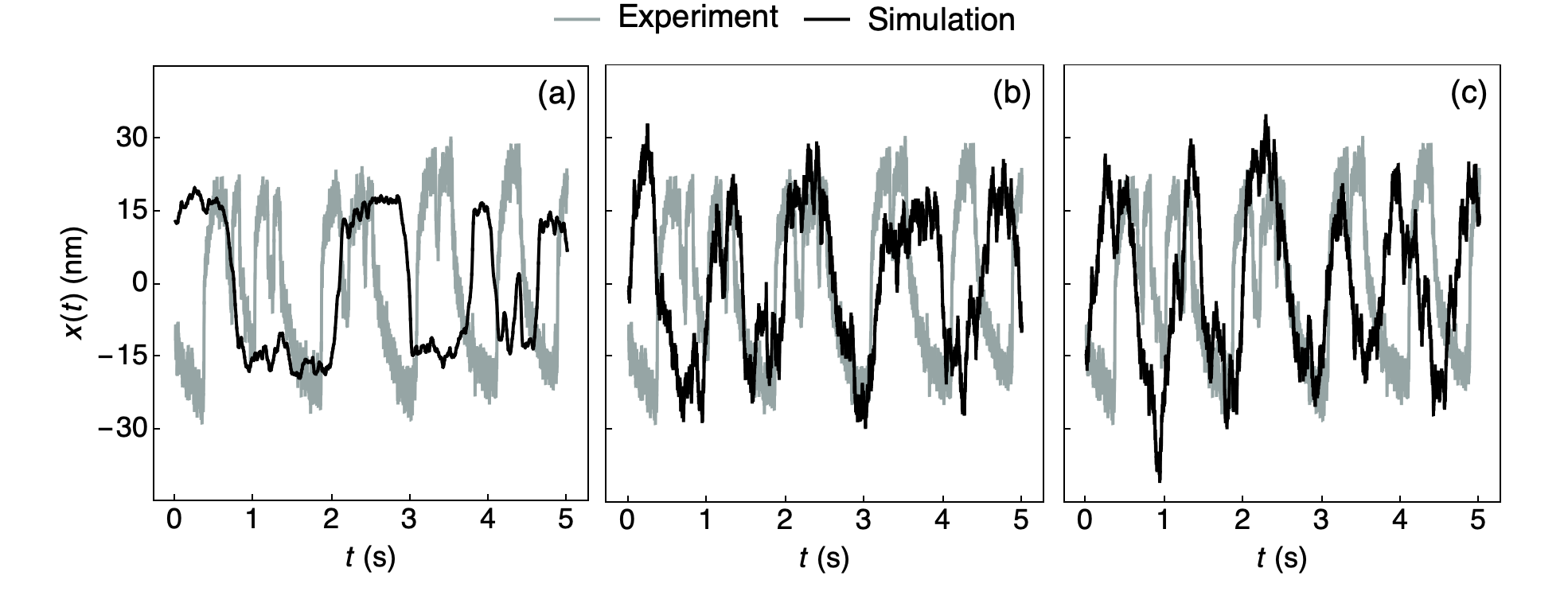
Figure 2: Comparision of three models for hair-cell bundle oscillations with the experimental data. Panel (a): The simple Van der Pol Eq. (1) does not reproduce oscillatory features of the experimental measurements. Panel (b): The hidden Van der Pol Eqs. (20)–(21) capture the general character of the hair bundle’s oscillations. Panel (c): The effective linear Eqs. (20) and (64) generally agree with the experimental data, but overestimate slightly the peak values of hair bundle’s noisy oscillations.

By using few simplifying assumptions, the alternative models mentioned above Nadrowski et al. (2004); Tinevez et al. (2007); Barral et al. (2010); O Maoileidigh et al. (2012) can be reduced to a form that is directly related to Eq. (1). A convenient scheme is a linear coupling between the coordinate $x(t)$ and a hidden Van der Pol oscillator $z(t)$. For a detailed demonstration of our approach we choose a simple scheme that is based on a parsimonious model of Ref. O Maoileidigh et al. (2012):

$$\dot{x}=\dot{z}+c_{x}z,$$ (20)

$$\ddot{z}+a\dot{z}+bz+c\dot{z}z^{2}=A\ddot{w},$$ (21)

in which $c_{x}$ is the coupling constant, whereas $a$, $b$, and $c$ are analogous to Eq. (1). Note the double overdot on the right-hand side of Eq. (21). We spare the mathematical and numerical details of Eqs. (20) and (21) for Appendix D.

Extension of the theory presented in Sec. II is quite straightforward. Because our example regards a drastic approximation of the original system, for simplicity we provide below only the formulas derived from the zeroth-order approximation of the Van der Pol limit cycle [Eq. (29)]. For the hair bundle’s position we obtain an equation analogous to (13):

$$x(t)\simeq\zeta(t)+\tilde{\zeta}(t),$$ (22)

in which $\zeta(t)$ and $\tilde{\zeta}(t)$ are the autonomous and the linear-response terms analogous to $\xi(t)$ and $\tilde{\gamma}(t)$. Instead of Eq. (16) we obtain from (20) and (29)

$$\zeta(t-t_{0})=\alpha\cos[\sqrt{b}(t-t_{0})]+\alpha c_{x}\int_{0}^{t-t_{0}}ds\cos(\sqrt{b}s)\\ =\tilde{\alpha}_{c}\cos(\sqrt{b}t)+\tilde{\alpha}_{s}\sin(\sqrt{b}t),$$ (23)

in which $\tilde{\alpha}_{c}=\alpha_{c}-\kappa\alpha_{s}$, $\tilde{\alpha}_{s}=\alpha_{s}+\kappa\alpha_{c}$, $\kappa=c_{x}/\sqrt{b}$; and instead of Eq. (15) we get

$$\tilde{\chi}(t)=\frac{\lambda_{1}^{2}}{\lambda_{1}^{2}+\lambda_{2}^{2}}\cos(\omega t)+\frac{\lambda_{2}^{2}}{\lambda_{1}^{2}+\lambda_{2}^{2}}\\ \times\exp\left(-\frac{\mu\omega t}{2}\right)\left[\cos\left(\sqrt{4-\mu^{2}}\frac{\omega t}{2}\right)\right.\\ \left.+\frac{\mu(\kappa^{2}-1)}{\sqrt{4-\mu^{2}}(\kappa^{2}+1)}\sin\left(\sqrt{4-\mu^{2}}\frac{\omega t}{2}\right)\right].$$ (24)

In addition we must replace the expression for $\alpha$ and $A$ in Eq. (18) by

$$\alpha = \sqrt{\frac{\tilde{\alpha}_{c}^{2}+\tilde{\alpha}_{s}^{2}}{(1+\kappa^{2})}},$$ (25)

$$A = \sqrt{-a\left(\frac{2\langle x^{2}\rangle}{1+\kappa^{2}}-\alpha^{2}\right)}.$$ (26)

By fitting the empirical autocorrelations and the oscillatory trend of the experimental measurements with the above formulas, we can infer all the parameter values for Eqs. (20) and (21). As illustrated in Fig. 2(b), these dynamical equations reproduce closely the character of the hair bundle’s oscillations and their frequency, despite the strong assumptions used to simplify the original model of Ref. O Maoileidigh et al. (2012).

Finally, as anticipated in Sec. II.1, we present below an effective linear model that imitates the self-sustained oscillations generated by the nonlinear system of Eqs. (20) and (21). One may recognize that the Gaussian term $\tilde{\zeta}(t)$ in Eq. (22) [as well as $\tilde{\gamma}(t)$ in Eq. (13)] represents a harmonic oscillator driven by a white-noise signal. If we apply to this oscillator a specifically designed deterministic force, in addition to the stochastic fluctuations we can elicit a response composed of the same Fourier modes that are present in the term $\zeta(t)$ [or $\xi(t)$].

The above program is implemented by coupling Eq. (20) to (64) that is derived in Appendix D. The exact steady-state solution of this linear system, whose simulation is compared with the experimental data in Fig. 2(c), is then given by Equation (22). The time series of the dynamical Eqs. (20) and (64) are nearly indistinguishable from the original system (20)–(21).

The empirical time autocorrelation functions of the experimental system and the three models discussed above are compared in Fig. 3. The Van der Pol oscillator does not match the observations at all, whereas the system with the hidden Van der Pol oscillator and its linear imitation reproduce the oscillatory features of the hair bundle movements quite well.

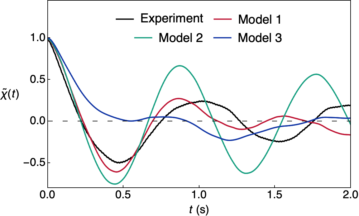
Figure 3: Comparison of the empirical time autocorrelation function $\tilde{\chi}(t)$ between the expeirments and the three theoretical models: 1 – the hidden Van der Pol Eqs. (20) and (21), 2 – the effective linear Eqs.  (20) and (64), 3 – the simple Van der Pol Eq. (1).

More advanced models of the hair-cell bundle oscillations can also be analyzed with help of the methods proposed in this paper. These developments, which require additional mathematical details, will be a subject of our future communications.

V Conclusion

Using the Volterra series we have analyzed statistical features of a noisy Van der Pol equation. Perhaps surprisingly, its solution can be decomposed within the linear order of the driving force into two independent contributions: a deterministic part that describes relaxation oscillations, and a stochastic linear-response term. With the help of simple approximation schemes we showed that the deterministic contribution has a singular probability density, whereas the stochastic part can be described by a Gaussian process with a second-order autocorrelation function.

Volterra series provide a representation of solutions for nonlinear stochastic equations. Other theoretical approaches, such as the Fokker-Planck equation and path integrals, focus instead on statistical properties of an ensemble of systems’ realizations and offer less information about their dynamics. The theoretical tools may complement each other; for instance, the Volterra series may be used to an advantage in ergodic problems when time averaging is more convenient than ensemble averaging for the evaluation of statistical properties.

The inference method based on our analytical results allows us to estimate parameter values of the stochastic Van der Pol model from observed time series of oscillations for moderate levels of the driving noise. However, due to the approximate nature of our theoretical expressions, this method cannot determine accurately values of small noise amplitudes. Two problems pose the major challenge for the Volterra-series approach here: finding a faithful representation of the Van der Pol limit-cycle solution and modeling the fluctuating phase of noisy oscillations. The latter issue is perhaps more pressing. A viable approach to the problem of fluctuating phase could be to study Eq. (1) in polar coordinates Raphael (1993).

In a simplified case study we have demonstrated that our theory can be applied to analyze actual physical systems. In particular, the Volterra-series approach offers a method of constructing a linear model that imitates the dynamics of self-sustatined oscillations. Albeit approximate, this imitation can be used to simplify quantitative studies of complex systems.

Appendices

Appendix A Limit-cycle solution of the autonomous Van der Pol oscillator

In this appendix we derive two levels of approximation for the limit-cycle solution of the autonomous Van der Pol problem. Although these two expressions can be obtained by using the harmonic-balance and Lindstedt-Poincare methods, we adopt here a unifying variational Green’s-function approach, which is similar in spirit to that of Refs. Khuri and Sayfy (2017); Abukhaled (2017). Equation (4) that we are solving can be recast as

$$\mathcal{L}_{\omega}x_{0}=-a\dot{x}_{0}-(b-\omega^{2})x_{0}-c\dot{x}_{0}x_{0}^{2},$$ (27)

in which $\mathcal{L}_{\omega}=\partial_{t}^{2}+\omega^{2}$ is a linear differential operator with a constant frequency parameter $\omega>0$. As in the harmonic-balance and Lindstedt-Poincare methods (Jordan and Smith, 2007, Sec. 4.4 and 5.9), we use the initial condition $\Big{(}x_{0}(0),\,\dot{x}_{0}(0)\Big{)}=(\alpha,\,0)$ with $\alpha$ left unspecified. The solution of Eq. (27) must then satisfy

$$x_{0}(t)= \xi_{0}(t)-\int_{0}^{t}g_{\omega}(t-s)$$

$$\times[a\dot{x}_{0}(s)+(b-\omega^{2})x_{0}(s)+c\dot{x}_{0}(s)x_{0}^{2}(s)]$$

$$= \alpha\cos(\omega t)-\frac{\sin(\omega t)}{\omega}\int_{0}^{t}\cos(\omega s)$$

$$\times[a\dot{x}_{0}(s)+(b-\omega^{2})x_{0}(s)+c\dot{x}_{0}(s)x_{0}^{2}(s)]$$

$$+\frac{\cos(\omega t)}{\omega}\int_{0}^{t}\sin(\omega s)$$

$$\times[a\dot{x}_{0}(s)+(b-\omega^{2})x_{0}(s)+c\dot{x}_{0}(s)x_{0}^{2}(s)],$$ (28)

in which $\xi_{0}(t)=\alpha\cos(\omega t)$ solves the equation $\mathcal{L}_{\omega}\xi_{0}=0$, whereas $g_{\omega}(t)=\sin(\omega t)/\omega$ is the Green function associated with the operator $\mathcal{L}_{\omega}$.

In the first approximation we posit a single-mode Fourier expansion $x_{0}(t)\approx\xi_{0}(t)$. For the right-hand side of Eq. (A) to satisfy the periodic boundary condition $x(0)=x(2\pi/\omega)$, one must choose:

$$\xi_{0}(t)=\alpha\cos(\sqrt{b}t)$$ (29)

with $\alpha=2\sqrt{-a/c}$. Alternatively this solution can be obtained by the method of harmonic balance (Jordan and Smith, 2007, Sec. 4.4).

The single-mode solution $\xi_{0}(t)$ can be further improved by one Picard iteration: we substitute $\xi_{0}(t)$ for $x_{0}(t)$ on the right-hand side of Eq. (A) and complete the integration to get

$$\xi_{1}(t)=\alpha\left[\cos(\sqrt{b}t)+\frac{3\mu}{8}\sin(\sqrt{b}t)-\frac{\mu}{8}\sin(3\sqrt{b}t)\right].$$ (30)

The above expression coincides with the perturbative solution that can be obtained by the Lindstedt-Poincare method of two time scales within the linear order of the parameter $\mu=-a/\sqrt{b}$ (Sec. III). With respect to this parameter, Eq. (A) represents the zeroth-order approximation of the limit cycle.

The two-timing solution $\xi_{1}(t)$ reproduces better the asymmetric trajectory of the Van der Pol limit cycle (Fig. 4) than $\xi_{0}(t)$. Both Eqs. (29) and (30) have the same frequency of oscillation $\omega=\sqrt{b}[1+O(\mu^{2})]$, whose corrections are of quadratic order in the parameter $\mu$ (Strogatz, 2014, Sec. 7.6). As discussed in the following Appendix, Eq. (29) is more convenient to describe time-invariant statistics of the response terms $\xi(t)$ and $\gamma_{\xi}$ in Eq. (13), whereas Eq. (30) yields a more accurate expression for the time autocorrelation function.

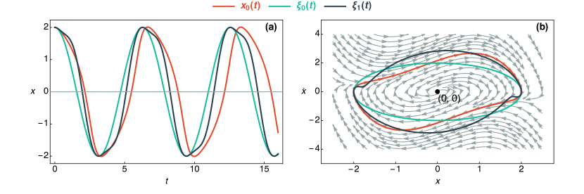
Figure 4: Comparison of the approximate solution $\xi_{0}(t)$ and $\xi_{1}(t)$ given by Eqs. (29) and (30), respectively, with a simulation of the autonomous Van der Pol Eq. (4): (a) time series of the limit-cycle solution (b) orbit of the oscillator’s limit cycle in the phase space $(x_{0},\,\dot{x}_{0})$. The simulation parameters are $\mu=1$, $A=0$, $\Big{(}x_{0}(0),\,\dot{x}_{0}(0)\Big{)}=(2,\,0)$ (Appendix C). The two approximate expressions match the simulated trajectory in panel (a) over a time interval of one period $t\lesssim 2\pi/\sqrt{b}\approx 6.28$. However, the asymmetric features of the oscillator’s limit cycle are reproduced only by Eq. (30).

Appendix B Statistical properties of noisy relaxation oscillations

Even in the absence of the external force $f(t)$ in Eq. (1), relaxation oscillations of the Van der Pol oscillator have nontrivial statistics. In the case of the zeroth-order approximate solution $x_{0}(t)\approx\xi_{0}(t)$ [Eq. (29)] we can find an exact probability distribution $p(\xi_{0})$, which is given by the arcsine law (Balakrishnan and Nevzorov, 2004, Chapters 16 and 17)—a special case of beta distributions with the support interval shifted by $-1/2$ and scaled by $2\alpha$:

$$p(\xi_{0})=\frac{d}{\pi d\xi_{0}}\left[\arcsin\left(\frac{\xi_{0}}{\alpha}\right)-\frac{\pi}{2}\right]=\frac{(\pi\alpha)^{-1}}{\sqrt{1-\xi_{0}^{2}/\alpha}}.$$ (31)

Statistics of $\xi_{0}(t)$ can also be evaluated by time averaging

$$\langle\xi_{0}\rangle=\int_{0}^{2\pi/\sqrt{b}}\frac{\sqrt{b}ds}{2\pi}\xi_{0}(s)=0,\quad\langle\xi_{0}^{2}\rangle=\frac{\alpha^{2}}{2},$$ (32)

$$\langle\xi_{0}(0)\xi_{0}(t)\rangle=\int_{0}^{2\pi/\sqrt{b}}\frac{\sqrt{b}ds}{2\pi}\xi_{0}(s)\xi_{0}(s+t)$$

$$\qquad=\langle\xi_{0}^{2}\rangle\cos(\sqrt{b}t)$$ . (33)

The probability density of $\xi_{0}(t)$ has two singularities at the ends of its support interval $\xi_{0}=\pm\alpha$. Histograms of the time series $\xi_{0}(t)$, as well as of $x_{0}(t)$, have two distribution modes near these points. In the companion paper Belousov et al. (2019) we have succeeded in fitting a bimodal probability density of the noisy Duffing oscillator to an approximate expression that was derived from a power series for the exponential family of random variables. This approach unfortunately fails in the case of the noisy Van der Pol oscillator: such an expansion may not exist near the two singularities at which $p(\xi_{0})$ tends to infinity.

For the probability density of $x_{\xi}(t)$ [Eq. (13)], regarded as the sum of two independent variables $\xi(t)\simeq\xi_{0}(t)$ and $\tilde{\gamma}(t)$, there is no simple analytical expression. However the Fourier image $\eta(X_{\xi})$—the characteristic function of $x_{\xi}$ for the reciprocal variable $X_{\xi}$—can be obtained in a closed form. Because $\tilde{\gamma}(t)$ is Gaussian, we have

$$\eta(X_{\xi})=\langle\operatorname{\mathrm{e}}^{\operatorname{\mathrm{i}}X_{\xi}x_{\xi}}\rangle=J_{0}(\alpha X_{\xi})\exp\left(-\frac{A^{2}X_{\xi}^{2}}{4\langle a_{\xi}\rangle\langle b_{\xi}\rangle}\right),$$ (34)

in which

$$J_{0}(\alpha X_{\xi})=\int_{0}^{2\pi/\sqrt{b}}\frac{\sqrt{b}ds}{2\pi}\operatorname{\mathrm{e}}^{\operatorname{\mathrm{i}}X_{\xi}\xi_{0}(s)}$$

is the characteristic function of $\xi_{0}(t)$ with $J_{0}(\cdot)$ being the zeroth-order Bessel function of the first kind. Using $\xi(t)\simeq\xi_{0}(t)$ in Eqs. (9) and (10) we get $\langle a_{\xi}\rangle\approx-a$ and $\langle b_{\xi}\rangle=b$.

In Fig. 5 we compare the empirical characteristic function of $x(t)$ with Eq. (34) for two representative examples. Our analytical expression for $\eta(X_{\xi})$ is accurate at least for $X_{\xi}\lesssim\langle x\rangle^{-1/2}$ even for large noise amplitudes $A$. The theory is in excellent agreement with the simulations for $A\equiv 0$.

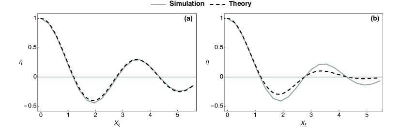
Figure 5: Comparison of the theoretical expression given by Eq. (34) with the empirical characteristic function $\eta(X_{\xi})$ obtained by simulating the Van der Pol Eq. (1). The system parameters are: (a) $\mu=1$, $A=0.0$ and (b) $\mu=1$, $A=0.6$. In these examples the theory is accurate at least for $X_{\xi}\lesssim\langle x^{2}\rangle^{-1/2}\approx 0.7$.

Although we have not obtained analytical expressions analogous to Eqs. (31) and (34) for the first-order approximate solution $\xi_{1}(t)$, its autocovariance function can be evaluated by time averaging:

$$\langle\xi_{1}(0)\xi_{1}(t)\rangle=\int_{0}^{2\pi/\sqrt{b}}\frac{\sqrt{b}ds}{2\pi}\xi_{1}(s)\xi_{1}(s+t)\\ =\langle\xi_{1}^{2}\rangle\frac{\cos(\sqrt{b}t)}{1+5\mu^{2}/32}\left\{1+\frac{\mu^{2}}{32}[4+\cos(2\sqrt{b}t)]\right\},$$ (35)

in which $\langle\xi_{1}^{2}\rangle=(1+5\mu^{2}/32)\alpha^{2}/2$.

Our simulations show that the theoretical expressions based on the linear-order approximation $\xi(t)\simeq\xi_{1}(t)$ overestimate the variance of the autonomous term $x_{0}(t)$, as well as of the noisy oscillations $x(t)$. This discrepancy might be caused by a broader orbit of $\xi_{1}(t)$ in the phase space, as compared to $x_{0}(t)$ and $\xi_{0}(t)$ [Fig. 4(b)]. Because the solution $\xi_{0}(t)$ provides a more accurate estimate of the variance $\langle x_{0}^{2}\rangle$, Eq. (18) is based on (29).

Because the terms $\xi(t)$ and $\tilde{\gamma}(t)$ in Eq. (13) are statistically independent, the autocorrelation function of $x_{\xi}(t)$ is given simply by

$$\chi_{\xi}(t)=\frac{\langle x_{\xi}(0)x_{\xi}(t)\rangle}{\langle x_{\xi}^{2}\rangle}=\frac{\langle\xi(0)\xi(t)\rangle+\langle\tilde{\gamma}(0)\tilde{\gamma}(t)\rangle}{\langle\xi^{2}\rangle+\langle\tilde{\gamma}^{2}\rangle}.$$ (36)

Approximating $\xi(t)$ by $\xi_{0}(t)$ and $\xi_{1}(t)$ we obtain, respectively,

$$\chi_{0}(t) = \frac{\langle\xi_{0}^{2}\rangle}{\langle\xi_{0}^{2}\rangle+\langle\tilde{\gamma}_{0}^{2}\rangle}\cos(\sqrt{b}t)+\frac{\langle\tilde{\gamma}_{0}^{2}\rangle}{\langle\xi_{0}^{2}\rangle+\langle\tilde{\gamma}_{0}^{2}\rangle}$$ (37)

$$\times \operatorname{\mathrm{e}}^{-\frac{a_{0}t}{2}}\left[\cos(\Omega_{0}t)+\frac{a_{0}}{2\Omega_{0}}\sin(\Omega_{0}t)\right],$$

$$\chi_{1}(t) = \frac{\langle\xi_{1}^{2}\rangle}{\langle\xi_{1}^{2}\rangle+\langle\tilde{\gamma}_{1}^{2}\rangle}\times\frac{\cos(\sqrt{b}t)}{1+5\mu^{2}/32}$$ (38)

$$\times \left\{1+\frac{\mu^{2}}{32}[4+\cos(2\sqrt{b}t)]\right\}+\frac{\langle\tilde{\gamma}_{1}^{2}\rangle}{\langle\xi_{1}^{2}\rangle+\langle\tilde{\gamma}_{1}^{2}\rangle}$$

$$\times \operatorname{\mathrm{e}}^{-\frac{a_{1}t}{2}}\left[\cos(\Omega_{1}t)+\frac{a_{1}}{2\Omega_{1}}\sin(\Omega_{1}t)\right],$$

in which

$$a_{0}=\mu\sqrt{b}, a_{1}=\mu\sqrt{b}(1+5\mu^{2}/16),$$ (39)

$$\Omega_{0}=\sqrt{b^{2}-a_{0}^{2}/4}, \Omega_{1}=\sqrt{b^{2}-a_{1}^{2}/4},$$ (40)

$$\langle\tilde{\gamma}_{0}^{2}\rangle=\frac{A^{2}}{2a_{0}b} \langle\tilde{\gamma}_{1}^{2}\rangle=\frac{A^{2}}{2a_{1}b}.$$ (41)

In Fig. 6 the empirical autocorrelation function $\chi(t)$ obtained from simulations of Eq. (1) is compared with the theoretical curve $\chi_{1}(t)$. To avoid redundancy, we do not reproduce the plot of $\chi_{0}(t)$ [Eq. (37)], which is almost indistinguishable from that of $\chi_{1}(t)$. Our theoretical expression predicts well the initial decay of the empirical time autocorrelation function, although a moderate phase difference accumulates at longer times.

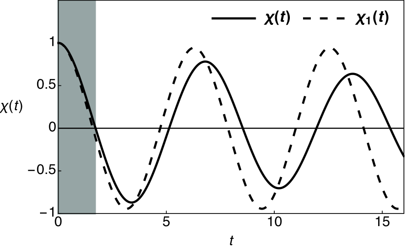
Figure 6: Comparison of the theoretical expression $\chi_{1}(t)$ [Eq. (1)] with the empirical time autocorrelation function $\chi(t)$ obtained from simulations of the Van der Pol Eq. (1). The system parameters are $\mu=1$, $A=0.6$. The agreement is good in the shaded region selected by the criterion of Lagarkov and Sergeev (Sec. II.2).

As discussed in Sec. II.1, the approximate Eq. (13) does not account for the fluctuating phase shift of the noisy oscillations that occur in presence of the driving force $f(t)$ and vanish as $A\to 0$. These stochastic phase variations accumulate slowly and decorrelate the time series of $x(t)$. Consequently the empirical autocorrelation function $\chi(t)$ decays to zero as $t\to\infty$ (Fig. 6) unless $f(t)\equiv 0$. This decay becomes faster as the noise amplitude $A$ increases. The persistent periodic terms $\propto\cos^{2}(\sqrt{b}t)$ in Eqs. (37) and (38), whose amplitude is constant, are therefore accurate only at small time scales.

Although graphs of Eqs. (37) (not reproduced in Fig. 6) and (38) are indistinguishable, fitting the latter expression to empirical time autocorrelations (Sec. II.2) performs better, because it provides tighter constraints on the parameter $\mu$. Fitting Eq. (37), in which the first term $\propto\cos^{2}(\sqrt{b}t)$ depends only on the parameter $b$, yields less accurate estimates of the constant $\mu$.

Appendix C Simulation algorithm

In our computational experiments we use a companion system of Eq. (1) with $\bm{X}=(x,y)=(x,\dot{x})$:

$$\begin{cases}\dot{x}=y\\ \dot{y}=-(a+cx^{2})y-bx+f(t)\end{cases}.$$ (42)

We adopt a second-order operator-splitting approach Tuckerman et al. (1992) for stochastic systems (Belousov et al., 2019, 2017, Appendix C), by decomposing the time-evolution operator $\mathcal{T}$ as

$$\dot{\bm{X}}=\mathcal{T}\bm{X}=(\mathcal{T}_{f}+\mathcal{T}_{y}+\mathcal{T}_{x})\bm{X},$$ (43)

in which

$$\mathcal{T}_{x}=y\bm{\partial_{x}},\;\mathcal{T}_{y}=-(a+cx^{2})y\bm{\partial_{y}},\;\mathcal{T}_{f}=(f-bx)\bm{\partial_{y}}.$$

The formal solution of Eq. (43) for a time step $\Delta{t}$

$$\bm{X}(t+\Delta{t})=\exp(\mathcal{T}\Delta{t})\bm{X}(t)$$

can be approximated by

$$\exp[\mathcal{T}\Delta{t}+\mathcal{O}(\Delta{t}^{2})]=\exp\left(\frac{\mathcal{T}_{x}\Delta{t}}{2}\right)\exp\left(\frac{\mathcal{T}_{y}\Delta{t}}{2}\right)\\ \times\exp(\mathcal{T}_{f}\Delta{t})\exp\left(\frac{\mathcal{T}_{y}\Delta{t}}{2}\right)\exp\left(\frac{\mathcal{T}_{x}\Delta{t}}{2}\right).$$ (44)

The action of individual operators of the form $\exp(\mathcal{L}\Delta{t})$ is determined by the differential equation

$$\dot{\bm{X}}(t)=\mathcal{L}\bm{X}(t)\Rightarrow\bm{X}(t+\Delta{t})=\exp(\mathcal{L}\Delta{t})\bm{X}(t).$$ (45)

The operators $T_{x}$, $T_{y}$, and $T_{f}$ produce linear equations of the above type and their action is given by

$$\operatorname{\mathrm{e}}^{\frac{t\mathcal{T}_{x}}{2}}(x,y)=\left(x+y\frac{\Delta{t}}{2},y\right),$$

$$\operatorname{\mathrm{e}}^{\frac{t\mathcal{T}_{y}}{2}}(x,y)=\left(x,y\operatorname{\mathrm{e}}^{-\frac{(a+cx^{)}\Delta{t}}{2}}\right),$$

$$\operatorname{\mathrm{e}}^{t\mathcal{T}_{f}}(x,z)=\left(x,y+bx^{2}\Delta{t}+\int_{0}^{\Delta{t}}ds\,f(s)\right).$$

For each value of the parameter $A$, the simulations reported in Sec. III involved $5\times 10^{5}$ time steps of a size $\Delta{t}=0.01$ in the reduced units. Statistics were calculated from single trajectories sampled at time intervals of $0.05$, which included $10^{5}$ observations.

Appendix D Hidden Van der Pol model for hair-bundle oscillations

In this appendix we reduce the parsimonious model of hair-bundle oscillations O Maoileidigh et al. (2012) to a simple form of a linear oscillator $x(t)$ coupled to a hidden Van der Pol oscillator $z(t)$ [Eqs. (20) and (21)]. The starting point of our derivation is a system of equations for $(x,y)$ (O Maoileidigh et al., 2012, cf. Eqs. (1) and (S6)):

$$M\ddot{x} = -\Gamma\dot{x}-K_{0}x+K_{1}(x-y)$$ (46)

$$- B_{0}(x-y)^{3}+F,$$

$$\tau_{0}\dot{y} = K_{2}x-K_{3}y,$$ (47)

in which $M$ and $x(t)$ are the mass and the position of the hair bundle, $y(t)$ is an adaptation coordinate, $K_{0}>0$, $K_{1}>0$, $K_{2}>0$, $K_{3}>0$, and $B_{0}>0$ are elastic constants, whereas $\Gamma>0$, $\tau_{0}>0$, and $F(t)$ are, respectively, a friction coefficient, a relaxation time of the adaptation coordinate $y$, and an external force.

We proceed by taking the overdamped limit of Eq. (46) $M/\Gamma\to 0$ and substituting a simplifying assumption $K_{2}\approx K_{3}$ into (47):

$$\dot{x} = -k_{0}x+k_{1}(x-y)-b_{0}(x-y)^{3}+f,$$ (48)

$$\dot{y} = c_{x}(x-y),$$ (49)

v, in which $k_{i=0,2}=K_{i=0,1}/\Gamma$, $c_{x}=K_{2}/\Gamma$, $b_{0}=B_{0}/\Gamma$, and $f(t)=F(t)/\Gamma$. Next we use a substitution of variables $z=x-y$, which transforms Eqs. (48) and (49) into

$$\dot{x}=-k_{0}x+k_{1}z-b_{0}z^{3}+f,$$ (50)

$$\dot{x}-\dot{z}=c_{x}z.$$ (51)

By subtracting the second of the above equations from the first one, we can recast our original system $(x,y)$ into a system $(x,z)$:

$$\dot{x} = -k_{0}x+k_{1}z-b_{0}z^{3}+f,$$ (52)

$$\dot{z} = -k_{0}x-(c_{x}-k_{1})z-b_{0}z^{3}+f.$$ (53)

Further, we use Eq. (53) and its time derivative to express $k_{0}x$ and $k_{0}\dot{x}$ as

$$k_{0}x = -\dot{z}-(c_{x}-k_{1})z-b_{0}z^{3}+f,$$ (54)

$$k_{0}\dot{x} = -\ddot{z}-(c_{x}-k_{1})\dot{z}-3b_{0}z^{2}\dot{z}+\dot{f}.$$ (55)

Then we use the above equations to eliminate $\dot{x}$ and $x$ from Eq. (52) and thus obtain

$$\ddot{z}+(k_{0}-k_{1}+c_{x})\dot{z}+k_{0}c_{x}z+3b_{0}z^{2}\dot{z}=\dot{f}.$$ (56)

If in the last equation we identify

$$a=k_{0}-k_{1}+c_{x},\quad b=k_{0}c_{x},\quad c=3b_{0},\quad f=a\dot{w},$$

we obtain Eq. (21)—the hidden Van der Pol oscillator. Equation (51) entails the linear coupling between $x(t)$ and $z(t)$ [Eq. (20)].

In simulations we integrate Eqs. (52) and (53) using a decomposition of the time evolution operator $\mathcal{T}$:

$$(\dot{x},\dot{z})=\mathcal{T}(x,z)=(\mathcal{T}_{f}+\mathcal{N}_{z}+\mathcal{L}_{z}+\mathcal{L}_{x})\bm{X},$$ (57)

in which

$$\mathcal{L}_{x}= (k_{1}z-b_{0}z^{3}-k_{0}x)\bm{\partial_{x}},$$ (58)

$$\mathcal{L}_{z}= -(k_{0}x+k_{z}z)\bm{\partial_{z}},$$ (59)

$$\mathcal{N}_{z}= -b_{0}z^{3}\bm{\partial_{z}},\;\mathcal{T}_{f}=f(\bm{\partial_{x}}+\bm{\partial_{z}}),\;$$ (60)

and $k_{z}=c_{x}-k_{1}$. Up to the second order in $t$ we then have

$$\operatorname{\mathrm{e}}^{t\mathcal{T}+\mathcal{O}(t^{2})}=\operatorname{\mathrm{e}}^{\frac{t\mathcal{L}_{x}}{2}}\operatorname{\mathrm{e}}^{\frac{t\mathcal{L}_{z}}{2}}\operatorname{\mathrm{e}}^{\frac{t\mathcal{N}_{z}}{2}}\operatorname{\mathrm{e}}^{t\mathcal{T}_{f}}\operatorname{\mathrm{e}}^{\frac{t\mathcal{N}_{z}}{2}}\operatorname{\mathrm{e}}^{\frac{t\mathcal{L}_{z}}{2}}\operatorname{\mathrm{e}}^{\frac{t\mathcal{L}_{x}}{2}},$$ (61)

in which the action of individual operators is

$$\operatorname{\mathrm{e}}^{\frac{t\mathcal{L}_{x}}{2}}(x,z)= \left(x\operatorname{\mathrm{e}}^{-\frac{k_{0}t}{2}}+\frac{k_{1}z-b_{0}z^{3}}{k_{0}}\left(1-\operatorname{\mathrm{e}}^{-\frac{k_{0}t}{2}}\right),z\right),$$

$$\operatorname{\mathrm{e}}^{\frac{t\mathcal{L}_{z}}{2}}(x,z)= \left(x,z\operatorname{\mathrm{e}}^{-\frac{k_{z}t}{2}}-\frac{k_{0}x}{k_{z}}\left(1-\operatorname{\mathrm{e}}^{-\frac{k_{z}t}{2}}\right)\right),$$

$$\operatorname{\mathrm{e}}^{\frac{t\mathcal{N}_{z}}{2}}(x,z)= \left(x,\frac{z}{\sqrt{1+z^{2}b_{0}t}}\right),$$

$$\operatorname{\mathrm{e}}^{t\mathcal{T}_{f}}(x,z)= \left(x+\int_{0}^{t}ds\,f,z+\int_{0}^{t}ds\,f\right).$$

As proposed in Sec. IV, the dynamical Eqs. (48)–(56) can be imitated by a driven harmonic oscillator. To implement this idea we replace the cubic nonlinear term of the original problem by a deterministic active force $f_{a}(t)=\alpha_{a}\cos(\omega_{a}t)+\beta_{a}\sin(\omega_{a}t)$ and a compensatory linear term $\Delta{k}(x-y)$ with real constants $\alpha_{a}$, $\beta_{a}$, $\omega_{a}$, $\Delta{k}$:

$$\dot{x} = -k_{0}x+k_{xy}(x-y)+f_{a}+f,$$ (62)

$$\dot{y} = c_{x}(x-y),$$ (63)

in which $k_{xy}=k_{1}+\Delta{k}$. By requiring that the steady-state solution of the above system is given by Eq. (22), we find

$$\alpha_{a}=\mu\sqrt{b}\alpha,\;\beta_{a}=0,\;\omega_{a}=\sqrt{b},\;k_{xy}=k_{0}+c_{x}-\mu\sqrt{b}.$$

Instead of Eq. (56) we then obtain

$$\ddot{z}+\mu\sqrt{b}\dot{z}+bz=\dot{f}_{a}+\dot{f},$$ (64)

whereas the linear coupling Eq. (20) remains unaltered.

References

- van der Pol (1926) B. van der Pol, The London, Edinburgh, and Dublin Philosophical Magazine and Journal of Science 2, 978 (1926).
- Ginoux and Letellier (2012) J.-M. Ginoux and C. Letellier, Chaos: An Interdisciplinary Journal of Nonlinear Science 22, 023120 (2012).
- Strogatz (2014) S. H. Strogatz, Nonlinear Dynamics and Chaos: With Applications to Physics, Biology, Chemistry, and Engineering, 2nd ed. (Avalon Publishing, 2014).
- Beta and Kruse (2017) C. Beta and K. Kruse, Annual Review of Condensed Matter Physics 8, 239 (2017).
- Oates et al. (2012) A. C. Oates, L. G. Morelli, and S. Ares, Development 139, 625 (2012).
- Buzsáki and Draguhn (2004) G. Buzsáki and A. Draguhn, Science 304, 1926 (2004).
- Nomura et al. (1993) T. Nomura, S. Sato, S. Doi, J. P. Segundo, and M. D. Stiber, Biological cybernetics 69, 429 (1993).
- Rompala et al. (2007) K. Rompala, R. Rand, and H. Howland, Communications in Nonlinear Science and Numerical Simulation 12, 794 (2007).
- Duifhuis et al. (1986) H. Duifhuis, H. W. Hoogstraten, S. M. van Netten, R. J. Diependaal, and W. Bialek, Peripheral Auditory Mechanisms, , 290 (1986).
- Talmadge et al. (1990) C. L. Talmadge, G. R. Long, W. J. Murphy, and A. Tubis, The Mechanics and Biophysics of Hearing, , 235 (1990).
- van Dijk and Wit (1990) P. van Dijk and H. P. Wit, The Journal of the Acoustical Society of America 88, 1779 (1990).
- van der Pol (1928) B. van der Pol, The London, Edinburgh, and Dublin Philosophical Magazine and Journal of Science 6, 763 (1928).
- van der Pol (1940) B. van der Pol, Acta Medica Scandinavica 103, 76 (1940).
- Mirollo and Strogatz (1990) R. E. Mirollo and S. H. Strogatz, SIAM Journal on Applied Mathematics 50, 1645 (1990).
- Cherevko et al. (2016) A. A. Cherevko, A. V. Mikhaylova, A. P. Chupakhin, I. V. Ufimtseva, A. L. Krivoshapkin, and K. Y. Orlov, Journal of Physics: Conference Series 722, 012045 (2016).
- Cherevko et al. (2017) A. A. Cherevko, E. E. Bord, A. K. Khe, V. A. Panarin, and K. J. Orlov, Journal of Physics: Conference Series 894, 012012 (2017).
- FitzHugh (1961) R. FitzHugh, Biophysical Journal 1, 445 (1961).
- Nagumo et al. (1962) J. Nagumo, S. Arimoto, and S. Yoshizawa, Proceedings of the IRE 50, 2061 (1962).
- Izhikevich and FitzHugh (2006) E. Izhikevich and R. FitzHugh, Scholarpedia 1, 1349 (2006).
- Alonso et al. (2014) R. Alonso, F. Goller, and G. B. Mindlin, Physical Review E 89 (2014), 10.1103/PhysRevE.89.032706.
- Mindlin (2017) G. B. Mindlin, Chaos: An Interdisciplinary Journal of Nonlinear Science 27, 092101 (2017).
- Roenneberg et al. (2008) T. Roenneberg, E. J. Chua, R. Bernardo, and E. Mendoza, Current Biology 18, R826 (2008).
- Belousov et al. (2019) R. Belousov, F. Berger, and A. J. Hudspeth, Physical Review E 99 (2019), 10.1103/physreve.99.042204.
- Schetzen (2006) M. Schetzen, The Volterra and Wiener Theories of Nonlinear Systems (Krieger Pub., 2006).
- Rugh (1981) W. J. Rugh, Nonlinear System Theory: The Volterra/Wiener Approach (Johns Hopkins University Press, 1981).
- Jordan and Smith (2007) D. Jordan and P. Smith, Nonlinear Ordinary Differential Equations:An Introduction for Scientists and Engineers: An Introduction for Scientists and Engineers (OUP Oxford, 2007).
- Grimshaw (2017) R. Grimshaw, Nonlinear ordinary differential equations (CRC Press, Boca Raton, 2017).
- Belousov and Cohen (2016) R. Belousov and E. G. D. Cohen, Physical Review E 94 (2016), 10.1103/PhysRevE.94.062124.
- Chandrasekhar (1943) S. Chandrasekhar, Rev. Mod. Phys. 15, 1 (1943).
- Lagar’kov and Sergeev (1978) A. N. Lagar’kov and V. M. Sergeev, Soviet Physics Uspekhi 21, 566 (1978).
- Hudspeth (2014) A. J. Hudspeth, Nature Reviews Neuroscience 15, 600 (2014).
- Martin and Hudspeth (1999) P. Martin and A. J. Hudspeth, Proceedings of the National Academy of Sciences 96, 14306 (1999).
- Faber and Bozovic (2018) J. Faber and D. Bozovic, Scientific Reports 8, 1 (2018).
- Nadrowski et al. (2004) B. Nadrowski, P. Martin, and F. Jülicher, Proceedings of the National Academy of Sciences 101, 12195 (2004).
- Tinevez et al. (2007) J.-Y. Tinevez, F. Jülicher, and P. Martin, Biophysical Journal 93, 4053 (2007).
- Barral et al. (2010) J. Barral, K. Dierkes, B. Lindner, F. Julicher, and P. Martin, Proceedings of the National Academy of Sciences 107, 8079 (2010).
- O Maoileidigh et al. (2012) D. O Maoileidigh, E. M. Nicola, and A. J. Hudspeth, Proceedings of the National Academy of Sciences 109, 1943 (2012).
- Azimzadeh and Salvi (2017) J. B. Azimzadeh and J. D. Salvi, JoVE (Journal of Visualized Experiments) , e55380 (2017).
- Azimzadeh et al. (2018) J. B. Azimzadeh, B. A. Fabella, N. R. Kastan, and A. J. Hudspeth, Neuron 97, 586 (2018).
- (40) These experiments were conducted in a sample chamber that was cooled down to 285 K by a peltier element and in accordance with the policies of The Rockefeller University’s Institutional Animal Care and Use Committee (IACUC Protocol 16942) .
- Gelfand et al. (2010) M. Gelfand, O. Piro, M. O. Magnasco, and A. J. Hudspeth, PLoS ONE 5, e11116 (2010).
- Raphael (1993) D. T. Raphael, The Journal of the Acoustical Society of America 94, 428 (1993).
- Khuri and Sayfy (2017) S. A. Khuri and A. Sayfy, , 9 (2017).
- Abukhaled (2017) M. Abukhaled, Journal of Computational and Nonlinear Dynamics 12, 051021 (2017).
- Balakrishnan and Nevzorov (2004) N. Balakrishnan and V. B. Nevzorov, A Primer on Statistical Distributions (John Wiley & Sons, 2004).
- Tuckerman et al. (1992) M. Tuckerman, B. J. Berne, and G. J. Martyna, The Journal of Chemical Physics 97, 1990 (1992).
- Belousov et al. (2017) R. Belousov, E. G. D. Cohen, and L. Rondoni, Physical Review E 96 (2017), 10.1103/PhysRevE.96.022125.