Normalised symmetric cumulants as a measure of QCD phase transition: a viscous hydrodynamic study
Abstract
Finding the existence and the location of the QCD critical point is one of the main goals of the RHIC beam energy scan program. To make theoretical predictions and corroborate with the experimental data requires modeling the space-time evolution of the matter created in heavy-ion collisions by dynamical models such as the relativistic hydrodynamics with an appropriate Equation of State (EoS). In the present exploratory study, we use a viscous 2+1 dimensional event-by-event (e-by-e) hydrodynamic code at finite baryon densities with two different EoSs (i) Lattice QCD + HRG with a crossover transition and (ii) EoS with a first-order phase transition to studying the normalized symmetric cumulants of charged pions . We show that the normalized symmetric cumulants can differentiate the two EoSs while all other conditions remain the same. The conclusion does not change for various initial conditions and shear viscosity. This indicates that these observables can be used to gain information about the QCD EoS from experimental data and can be used as an EoS meter.
I Introduction
It is well known that at low temperature and small baryon chemical potential, the degrees of freedom of nuclear matter are color-neutral hadrons; whereas at high temperature or large baryon chemical potential, the matter is in the form of quark-gluon plasma (QGP), in which the fundamental degrees of freedom are colored objects quarks and gluons. The nuclear matter at high baryon density and finite temperature are believed to undergo first-order phase transitions, from the hadronic phase to the QGP phase, and the first-order phase transition line terminates at a critical point Datta et al. (2013); Borsanyi et al. (2010); Gavai and Gupta (2005). This is because lattice QCD shows that the hadron to QGP transition is a crossover for vanishing baryon chemical potential at temperature 170 MeV Bernard et al. (2005); Bhattacharya et al. (2014); Borsanyi et al. (2010); Bazavov et al. (2012). For details on QCD phase diagram and critical points see review Fukushima and Hatsuda (2011); Baym et al. (2018)
Present theoretical models widely disagree with each other regarding the value of critical temperature and baryon chemical potential corresponding to the QCD critical point on the QCD phase diagram Schaefer et al. (2007); Kovacs and Szep (2008). Also, the existence of the QCD critical point is yet to be confirmed experimentally Aggarwal et al. (2010); Adamczyk et al. (2014a, b, 2018); Luo (2015); Mohanty (2009). It is crucial that phenomenologically motivated studies of the heavy-ion collision, such as relativistic hydrodynamics, be capable of accounting for the potential influence of such a critical point on experimental observables. Recently it was shown Pang et al. (2018) that the goal mentioned above can be achieved by using relativistic hydrodynamic model, experimental data and a state-of-the-art deep-learning technique that uses a convolutional neural network to train the system.
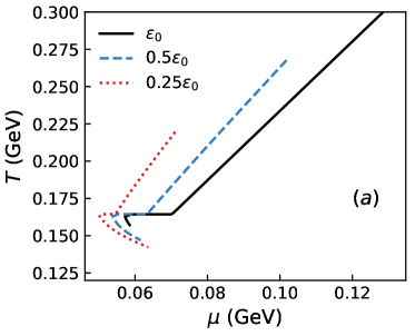
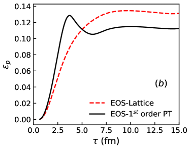
The present exploratory study aims to find a unique observable which connects QCD Equation of State (EoS) and the experimental data of heavy-ion collisions using one of the available dynamical models. We believe this effort will be complementary to the finding of Pang et al. (2018). It is well known that the initial energy/baryon densities follow very different space-time trajectories in the QCD phase diagram for crossover and first-order phase transitions Stephanov et al. (1998). This fact is shown in Fig. 1(a), the three different lines correspond to different entropy per baryon numbers (), and the trajectory for the crossover will follow line. The first-order phase transition involves finite latent heat (kink in the trajectories), and the speed of sound is zero in the mixed-phase. We note that in the fluid dynamical picture, converting the initial spatial deformation to the final momentum anisotropy depends on the speed of sound (EOS) and other factors such as the viscosity of the medium. In the case of crossover, the speed of sound is never zero; the consequence of the two different EoS’s can be seen in the temporal evolution of momentum space anisotropy (defined later) shown in Fig. 1(b). A different value of corresponds to different elliptic flow. Although event averaged elliptic flow is sensitive to the EoS used, it is also known that its value is suppressed in the presence of finite shear viscosity. Therefore the event-averaged elliptic flow is not a good indicator of the EoS. Nevertheless, it is interesting to investigate what imprint of different EoSs one can find in the correlation between the initial fluctuating geometry and the final flow coefficients in the event-by-event collisions Niemi et al. (2013).
We use the relativistic hydrodynamic model which has been very successful in simulating heavy-ion collisions and explaining experimental observablesKolb et al. (2000); Nonaka et al. (2000); Hirano (2002); Aguiar et al. (2001); Chaudhuri (2006); Nonaka and Bass (2007); Song and Heinz (2008a); Baier and Romatschke (2007); Muronga (2007); Pratt and Vredevoogd (2008); Petersen et al. (2008); Molnar et al. (2010); Schenke et al. (2010); Werner et al. (2010); Holopainen et al. (2011); Roy and Chaudhuri (2012); Bozek (2012); Pang et al. (2012); Akamatsu et al. (2014); Noronha-Hostler et al. (2013); Del Zanna et al. (2013). We find the linear/Pearson correlation (defined later) of initial geometric asymmetry to the corresponding flow coefficient (particularly the second-order flow coefficient ) is a unique observable which can differentiate between EoS with a first-order phase transition to that with a crossover transition irrespective of the initial condition used. It has been known that the event averaged and the eccentricity of the averaged initial state, are approximately linearly correlated Niemi et al. (2013); Plumari et al. (2015); Kolb and Heinz (2003); Song and Heinz (2008b),and the initial condition used Niemi et al. (2013). Although the above finding sounds promising, we need to keep in mind that the initial eccentricities are not directly measurable in experiments; hence the correlation between the eccentricities and flow coefficients may not provide any practical information about the EoS’s. But we can use the cumulants between flow coefficients such as and Adam et al. (2016); Bilandzic et al. (2014) which can always be measured experimentally without referring to any particular model. That is what motivates us to investigate these observables described above as an EoS meter.
For the present study, we use a newly developed -dimensional event-by-event viscous hydrodynamic code with an EoS Kolb et al. (2000) with finite baryon chemical potential/density for low collisions, and a lattice QCD+HRG EoS Huovinen and Petreczky (2010) for the higher collisions. There are ongoing efforts to construct EoS with a critical point Plumberg et al. (2018); Monnai et al. (2019). Due to the present uncertainty in the location of QCD critical point, we refrain to use sophisticated EoSs.
The conservation equations are solved numerically by using the time-honored SHarp And Smooth Transport Algorithm (SHASTA) Boris and Book (1973). In the next section, we shall discuss the details of various tests performed to find the numerical accuracy of the code. As we will show, our code passes all the test cases satisfactorily.
The paper is organized as follows: in the next section, we discuss various aspects of the newly developed hydrodynamic code. In section II we show the comparison of experimental data of charged pion invariant yield and elliptic flow in Au+Au 200 GeV collisions to the simulation result for optical Glauber initial condition to test the code. In the same section, we also discuss the correlation between different observable and the effect of EoS on them. Finally in section III we conclude and discuss some future possibilities. Throughout this article we adopt the units The signature of the metric tensor is always taken to be . Upper greek indices correspond to contravariant and lower greek indices covariant. The three vectors are denoted with Latin indices.
I.1 Conservation equations
Relativistic hydrodynamics model of high-energy heavy-ion collisions assumes that matter created in collisions reaches a state of local thermal equilibrium at time . The evolution of the thermalised nuclear matter is governed by the conservation equation of energy-momentum tensor and net baryon current,
| (1) | |||||
| (2) |
where the the energy-momentum tensor and the net baryon current can be expressed as
| (3) | |||||
| (4) |
Here is the local energy density, is pressure, is the metric tensor, is the net baryon density, is the time-like 4-velocity with and is the shear-stress tensor. The evolution equation for the shear-stress tensor is given as Denicol et al. (2012); Israel and Stewart (1976)
| (5) |
where is the shear viscosity coefficient, is the comoving time derivative, is the shear tensor, is the expansion rate, and , with . The transport coefficients in the above equation were obtsined in the massless limit with the relaxation time being .
In the present work, we will be using two kinds of EoS’s:
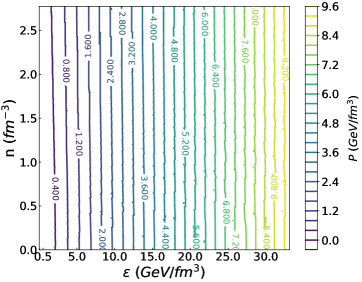
(i) A parameterized EoS Noronha-Hostler et al. (2019) shown in Fig. 2 (left panel) which has a cross-over transition between high temperature QGP phase obtained from lattice QCD and a hadron resonance gas below the crossover temperature. In order to have a smooth pressure profile as a function of and , the pressure is first expanded as a as a Taylor series in powers of . The associated Taylor coefficients which are known form LQCD Borsanyi et al. (2014); Bazavov et al. (2014) are parameterized using polynomial of ninth order.
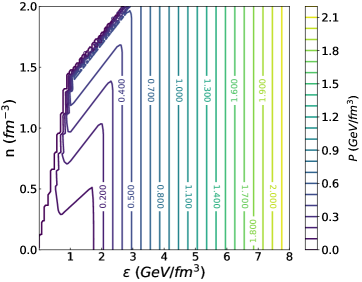
(ii) A parameterized EoS Kolb et al. (2000) with a first order phase transition at finite net baryon number density shown in Fig. 2 (right panel). The EoS connects a non-interacting massless QGP gas at high temperature to a hadron resonance gas, of masses up to 2 GeV, at low temperatures through a first order phase transition. The bag constant is a parameter adjusted to MeV, to yield a critical temperature of MeV. We note that the choice of bag parameter used here is not unique,
it may vary between MeV Baym et al. (2018). Both of these EoS will be used in the hydrodynamic simulation corresponding to 62.4 GeV collisions at a finite net baryon density.
Instead of solving the full dimensional hydrodynamics equations, we consider a simplified evolution by assuming boost invariant expansion in the direction. This can be done easily by working in the Milne coordinates with metric tensor given by . The velocity 4-vector in this coordinate (physical quantities in this coordinate is written with a tilde sign), , where and with .
Conservative equations of the form Eqs. (1,2,5) can be solved accurately using flux-corrected transport (FCT) algorithms Refs. Boris et al. (1993); Powell et al. (1999); Marti and Mueller (1999) without violating the positivity of mass and energy, particularly near shocks and other discontinuities. Here, we use the SHASTA (”SHarp and Smooth Transport Algorithm”), which is a designed to solve partial differential equations of the form
| (6) |
where is for example is the component of three-velocity, and is a source term. The local rest frame charge and energy densities are given as
| (7) | |||||
| (8) |
while the velocity components are calculated using an one-dimensional root search algorithm, by iterating the following transcendental equation
| (9) |
such that the components of velocity are given by
| (10) |
where . In this velocity finding algorithm we keep the accuracy .
We have tested our numerical simulation against dimensional Riemann problem which has an analytical solution in the perfect-fluid limit. The numerical solution reproduces the analytic solution with a very high precision with sufficiently high numerical resolution. We have similarly checked and verified the applicability of our numerical simulation to dimension by having the initial discontinuity in the dimensional Riemann problem in the plane . For small viscosities , we have verified that the viscous version of our simulation reproduces the result of our simulation with but with anti-diffusion coefficient , which is the numerical analog of physical viscosity. Finally, we have checked that our numerical simulation reproduces Gubser flow with initial condition fixed such that, the system expands and cools down much faster than typical heavy-ion collisions. In the numerical code we use the CORNELIUS subroutine reported in Huovinen and Petersen (2012). The subroutine uses an improved version of the original Marching Cube algorithm and extends the different distinct possible topological configuration from to and thus creates a consistent surface with lesser holes and no double counting which is required for event-by-event hydrodynamics study.
II Result
II.1 Testing for smooth Glauber
Before we show the result of event-by-event hydrodynamics simulation we show here the results from smooth optical Glauber model for , GeV collision energies respectively. For all the calculations, the spatial extension of the numerical grid is set to fm2. The spatial grid spacing is set to fm and the temporal spacing is set to fm. The initial time for all collisional erergies is fixed to fm.
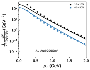
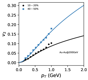
For Au-Au collisions at GeV we use EoS-Lattice shown in Fig. 2(a) with MeV and the freeze-out energy density is taken to be GeV/fm3 which corresponds to a temperature MeV. The central energy density is fixed to GeV/fm3 for collision centrality which explains the corresponding experimental data. The top panel of Fig. 3 shows the comparison of invariant yield of for and centrality collisions. Experimental data measured by PHENIX collaboration Adler et al. (2004) are shown by different symbols and the corresponding simulation results are shown by lines. We found reasonable agreement with the experimental data except at low momentum GeV, this is because we neglected the contribution of yield coming from various heavier resonance decay. We plan to incorporate the resonance decay in a later version of the code. The comparison of simulated elliptic flow with the experimental data of STAR collaboration Adams et al. (2005) are shown in the bottom panel of Fig. 3. We can see that the simulated result nicely explain the observed asymmetry in the final momentum spectra of .
For Au-Au collisions at GeV we use EoS- order PT shown in Fig. 2(b) and the freeze-out energy density is fixed to GeV/fm3. The initial central energy density is set to GeV/fm3 for collision centrality. Similarly, the initial central net baryon density is fixed to fm-3. We have checked that the above parameters explains the invariant yield of Back et al. (2007) across various centralities. In Fig. 1(a) we have plotted the trajectories of different regions of the fireball during hydrodynamical evolution as a function temperature () and net baryon chemical potential () with initial energy densities corresponding to 100, 50, 25 of the maximum energy density Gev/fm3 till freeze-out . The corresponding constant for the above lines are 156, 175 and 206 respectively. Momentum space anisotropy defined as
| (11) |
where are components of energy-momentum tensor are plotted in Fig. 1(b) both for EoS-Lattice and first order phase transition at fm. This completes the testing of our code. In the next section, we shall study the effect of phase transition on the various flow correlation which is the main goal of this paper.
II.2 Normalised symmetric cumulant and event-by-event flow correlation
Flow observables obtained from multiparticle correlations, symmetric cumulants (SC), are introduced, which are defined as Adam et al. (2016); Bilandzic et al. (2014)
| (12) | ||||
with the condition for two positive integers and . The double angular brackets indicate that the averaging procedure has been performed in two steps- first over all distinct particle quadruplets in an event, and then in the second step the single-event averages were weighted with number of combinations. The four-particle cumulant in Eq. (12) is less sensitive to non-flow correlations than any 2- or 4-particle correlator on the right-hand side taken individually Borghini et al. (2001a, b). The last equality is true only in the absence of non-flow effects. The observable in Eq. (12) is zero in the absence of flow fluctuations, or if the magnitudes of harmonics and are uncorrelated. Experimentally it is more reliable to measure the higher order moments of flow harmonics with 2- and multiparticle correlation techniques, than to measure the first moments with the event plane method, due to systematic uncertainties involved in the event-by-event estimation of symmetry planes.
One can also define normalised symmetric cumulants (NSC) as,
| (13) |
Normalized symmetric cumulants reflect the strength of the correlation between and , while has contributions from both the correlations between the two different flow harmonics and the individual harmonics. In the present work, we calculate the symmetric cumulants using the last equality in Eq. (12), due to the absence of non-flow effects in our hydrodynamic formulation.
The hydrodynamics equation of motion has to be initialized at an initial time , by specifying the initial energy densities or the entropy densities and the flow velocities of a relativistic fluid. Two of such models that we are going to use are the Glauber model Miller et al. (2007) and the TRENTo model Moreland et al. (2015).
Given a pair of projectiles labeled and collide along the beam axis and let be the density of the nuclear matter that participate in inelastic collisions. is usually given by the Woods-Saxon profile, given as
| (14) |
where and are the normalization, size of the nucleus, and the stiffness of the edge of nucleon distribution profile respectively while are the spatial coordinates. Each projectile may then be represented by its participant thickness, given by
| (15) |
We shall assume that their exists a function which converts the projectile thickness to entropy production, namely . In a two-component Glauber model the function is the sum of , which is proportional to the number of wounded nucleons and a quadratic term , which is proportional to the number of binary collisions . The complete function is given as
| (16) |
The proportionality constants and the other relevant details can be found in Miller et al. (2007). However, in general the energy density profile in the reaction zone of nucleus-nucleus collision fluctuates from event to event due to the quantum fluctuations of the nuclear wave function. This fluctuations are attributed to the fluctuations in the positions of participating nucleons. In such a case, the previous decribed smooth Glauber distribution will then be an ensemble average of a large number of fluctuating initial distribution. This can be achieved by extending the smooth Glauber model to their Monte Carlo (MC) versions. These fluctuating initial distributions breaks the rotational and reflection symmetry of the smooth distributions.
The TRENTo model Moreland et al. (2015) for the initial condition assumes the a scale invariant form of the function , i.e.,
| (17) |
for any nonzero constant . One can clearly see that the above is broken by the binary collision term in the Glauber model. TRENTo assumes a reduced thickness function given by
| (18) |
Various limiting cases of the function , for different choices of parameter can be found in Moreland et al. (2015). In the present study we assume , in which case , which is the geometric mean of the and . We will be using the above two models in order to see the sensitivity of various correlations to the initial conditions used for the simulations.
We are interested in the study of the difference in fluid dynamical response of the system to the initial geometry (anisotropy) for two different EoS. In the literature this initial geometry/anisotropy of the overlap zone of two colliding nucleus is quantified in terms of eccentricities Alver and Roland (2010); Alver et al. (2010):
| (19) |
where is the spatial azimuthal angle, and is the participant angle given by,
| (20) |
is basically the eccentricity of a polygon of order, which can be reconstructed from a initial distribution generated from a MC Glauber or TRENTo model in a given event. Such a order initial distribution generates a order harmonic flow analogous to .
As described before, the azimuthal momentum anisotropy is characterized in terms of the coefficients of the Fourier expansion of the single particle azimuthal distribution. We use the following definition to calculate in each event:
| (21) |
In Eq. (21) can be calculated as the expectation , with respect to the associated event plane angle of -th order harmonics and is defined as
| (22) |
The angle brackets indicates the averaged value with respect to the particle spectrum.
Event-by-event hydrodynamics is one of the most natural way to model azimuthal momentum anisotropies Eq. (21) generated by fluctuating initial-state anisotropies Eq. (19), which are generated by the highly fluctuating initial conditions in experiments. The largest source of uncertainty in these hydrodynamic models are the initial conditions. Since, direct measurement of bulk properties of matter like EoS in experiments is not possible, we try to identify hydrodynamic responses which in one hand can be calculated in experiments and in other hand are also tolearant to uncertainities in the model parameters viz., the initial conditions, shear viscosity etc.
It has been known that the event averaged , and the eccentricity of the averaged initial state, are approximately linearly related Kolb and Heinz (2003); Song and Heinz (2008b) for but the same may not be true for higher-order flow coefficients. It is also known that the same linear relationship holds approximately between and even for event-by-event fluctuating conditions Niemi et al. (2013). Here we first study how the event-by-event correlation between and is changed when the system undergoes either a first phase transition or a cross over. In order to quantify the linear correlation we use Pearson’s correlation coefficient which is defined as
| (23) |
where and are the standard deviations of the quantities and . The correlation coefficient ranges from to . A value of implies that a linear (anti-linear) correlation between and . A value of implies that there is no linear correlation between the variables. In a previous study, it was shown that the Pearson correlator is almost insensitive to the different initial condition and the value of shear viscosity over entropy density of the fluid Niemi et al. (2013). Further, assuming an approximate linear relationship between the and , we can write for event-by-event case
| (24) |
where and the average error The values of indicate how efficiently the initial deformation is transformed into the final momentum anisotropy.
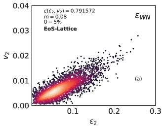
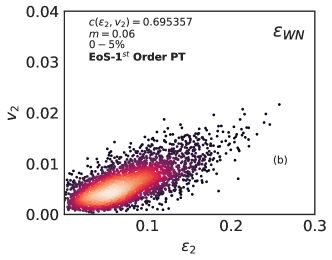
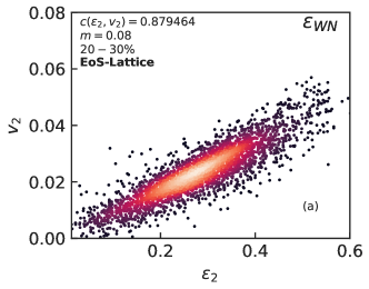
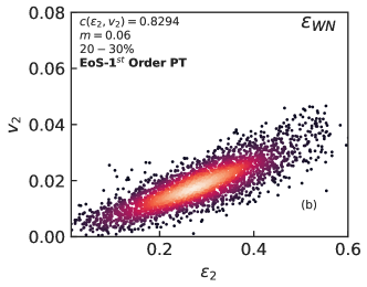
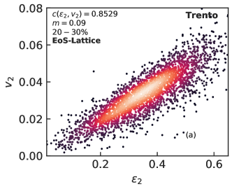
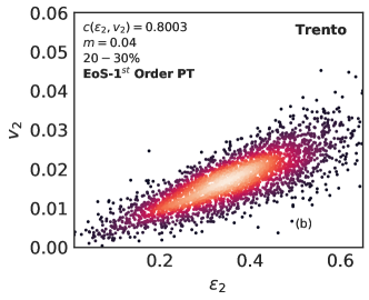
In Fig. (4) (a) (Top row) we show the event-by-event distribution of vs for Au+Au collisions at GeV. The initial energy density and are obtained from the MC-Glauber model with the contribution coming only from wounded nucleons. The result is obtained for EoS-Lattice, i.e, crossover transition. Fig. (4) (b) (Top row) shows the same, but with EoS having a first order phase transition. Using two different EoS we found decrease in for the case of first order phase transition, which clearly indicates that can be treated as a good signal of phase transition in the nuclear matter. Above results are not surprising since the speed of sound becomes zero (hence the expansion) for a certain temperature range in the first order phase transition. Fig. (4) (a,b) (Middle row and bottom row) shows the same results but for centrality using MC-Glauber and TRENTo model initial conditions. The first order phase transition shows a and decrease in the value of respectively. Thus, we infer that although, the value of for first-order phase transition is always less than that with crossover transition independent of the model used, the difference is more prominent in the central collisions than at higher centrality. Similarly, other higher order correlations e.g., , (for or ) is found to be smaller for the case of first order phase transition.
However, note that the initial eccentricities are not accessible in real experiments (and are model dependent) and hence the are not as interesting as which can be calculated from the available experimental data. As pointed out earlier instead of , a clean experimental observable would rather be the normalised symmetric cumulants .
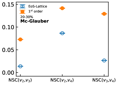
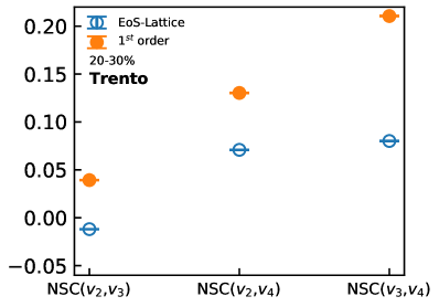
This EoS dependence of the flow correlations can be more clearly seen from NSC Fig. (5) (left panel), where we show , , and for EoS-Lattice (solid orange circles) and EoS first order phase transition (open blue circles) with corresponding errors for collision centrality. We have used the MC-Glauber initialisation. Fig.5 (right panel) shows the same but for TRENTo model. The errors are calculated by using bootstrap method. As can be seen from the Figs. (5) that the , , and always distinguishes the two different EoSs. These observations may be attributed to very different evolutionary dynamics of the system for the two different EoS, as the speed of sound becomes zero in first-order phase transition hence the linear/non-linear coupling of - and - is different in the two scenario. Although the absolute values of the varies for different initial condition (energy density scales with wounded nucleons or in the TRENTo model), the difference in them remains almost same for two different EoSs. We found in the mid central collisions is larger for the EoS with first order phase transition irrespective of the initial conditions used here.
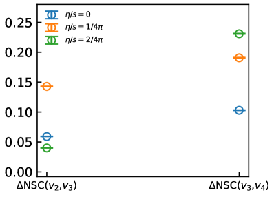
Finally, in order to see the influence of viscosity in the observables discussed above, we did the simulation for various values of . In Fig. (6), we show the difference between calculated for EoS- with first order phase transition and that with crossover. The initial energy density is obtained from wounded nucleons in MC-Glauber model for collision centrality. As in ideal hydrodynamics, the results of for first order phase transition are again larger than that with crossover. Increasing increases the difference between them for . The same is not true for , which is too sensitive to the shear viscosity and responds to it in a rather non-trivial manner.
This indicates that we can utilize to probe the EoS of the system which implies that one can possibly use this observable to locate the QCD critical point. For example we can calculate from available experimental data for various and pinpoint the energies where shows a sudden change in magnitude.
III Conclusion and outlook
In this paper, we studied correlation and for in ultra-relativistic heavy-ion collisions using event-by-event viscous fluid dynamics model for two different EoSs. The comparison of numerical results from the hydro code to the corresponding analytic solution in 1+1D and in 2+1D shows very good agreement between them. Using optical Glauber model as an initial condition, we confirm that our code nicely explains experimentally measured charged pion invariant yield and elliptic flow in Au+Au collision at 200 GeV and 62.4 GeV. First using ideal hydrodynamics with two different EoS’s we showed that the , and clearly distinguishes a first order phase transition scenario and a cross over transition. Although the absolute values of the varies for different initial condition (energy density scales with binary collisions or wounded nucleons) the difference in them remains almost same for two different EoSs. We found in the mid central collisions is larger for the EoS with first order phase transition irrespective of the initial conditions used here. In the presence of finite viscosity, the result that the value of is larger for EoS with first order phase still remains valid. However by inreasing the viscosity we found the difference between the results from first order phase transition and that with crossover increases for .
This indicates that we may utilize to probe the EoS of the system which implies that one can possibly use this observable to locate the QCD critical point. For example, we can calculate from available experimental data for various and pinpoint the energies where shows a sudden change in magnitude.
The coefficients can be directly calculated from the available experimental data, whereas calculation of requires input from an initial condition model hence proves to be less attractive observable than . However, we would like to point out that our study also shows is a promising observable for probing the EoS as it shows difference in the two scenarios.
Acknowledgement
We thank J.Y. Ollitrault and R. Bhalerao for suggestions and helpful discussion. V.R. is supported by the DST Inspire faculty research grant (IFA-16-PH-167), India. AD acknowledges financial support from DAE, Government of India.
References
- Datta et al. (2013) S. Datta, R. V. Gavai, and S. Gupta, Nucl. Phys. A 904-905, 883c (2013), arXiv:1210.6784 [hep-lat] .
- Borsanyi et al. (2010) S. Borsanyi, Z. Fodor, C. Hoelbling, S. D. Katz, S. Krieg, C. Ratti, and K. K. Szabo (Wuppertal-Budapest), JHEP 09, 073 (2010), arXiv:1005.3508 [hep-lat] .
- Gavai and Gupta (2005) R. V. Gavai and S. Gupta, Phys. Rev. D 71, 114014 (2005), arXiv:hep-lat/0412035 .
- Bernard et al. (2005) C. Bernard, T. Burch, E. B. Gregory, D. Toussaint, C. E. DeTar, J. Osborn, S. Gottlieb, U. M. Heller, and R. Sugar (MILC), Phys. Rev. D 71, 034504 (2005), arXiv:hep-lat/0405029 .
- Bhattacharya et al. (2014) T. Bhattacharya et al., Phys. Rev. Lett. 113, 082001 (2014), arXiv:1402.5175 [hep-lat] .
- Bazavov et al. (2012) A. Bazavov et al., Phys. Rev. D 85, 054503 (2012), arXiv:1111.1710 [hep-lat] .
- Fukushima and Hatsuda (2011) K. Fukushima and T. Hatsuda, Rept. Prog. Phys. 74, 014001 (2011), arXiv:1005.4814 [hep-ph] .
- Baym et al. (2018) G. Baym, T. Hatsuda, T. Kojo, P. D. Powell, Y. Song, and T. Takatsuka, Rept. Prog. Phys. 81, 056902 (2018), arXiv:1707.04966 [astro-ph.HE] .
- Schaefer et al. (2007) B.-J. Schaefer, J. M. Pawlowski, and J. Wambach, Phys. Rev. D 76, 074023 (2007), arXiv:0704.3234 [hep-ph] .
- Kovacs and Szep (2008) P. Kovacs and Z. Szep, Phys. Rev. D 77, 065016 (2008), arXiv:0710.1563 [hep-ph] .
- Aggarwal et al. (2010) M. M. Aggarwal et al. (STAR), Phys. Rev. Lett. 105, 022302 (2010), arXiv:1004.4959 [nucl-ex] .
- Adamczyk et al. (2014a) L. Adamczyk et al. (STAR), Phys. Rev. Lett. 112, 032302 (2014a), arXiv:1309.5681 [nucl-ex] .
- Adamczyk et al. (2014b) L. Adamczyk et al. (STAR), Phys. Rev. Lett. 113, 092301 (2014b), arXiv:1402.1558 [nucl-ex] .
- Adamczyk et al. (2018) L. Adamczyk et al. (STAR), Phys. Lett. B 785, 551 (2018), arXiv:1709.00773 [nucl-ex] .
- Luo (2015) X. Luo (STAR), PoS CPOD2014, 019 (2015), arXiv:1503.02558 [nucl-ex] .
- Mohanty (2009) B. Mohanty, Nucl. Phys. A 830, 899C (2009), arXiv:0907.4476 [nucl-ex] .
- Pang et al. (2018) L.-G. Pang, K. Zhou, N. Su, H. Petersen, H. Stöcker, and X.-N. Wang, Nature Commun. 9, 210 (2018), arXiv:1612.04262 [hep-ph] .
- Noronha-Hostler et al. (2019) J. Noronha-Hostler, P. Parotto, C. Ratti, and J. M. Stafford, Phys. Rev. C 100, 064910 (2019), arXiv:1902.06723 [hep-ph] .
- Stephanov et al. (1998) M. A. Stephanov, K. Rajagopal, and E. V. Shuryak, Phys. Rev. Lett. 81, 4816 (1998), arXiv:hep-ph/9806219 .
- Niemi et al. (2013) H. Niemi, G. S. Denicol, H. Holopainen, and P. Huovinen, Phys. Rev. C 87, 054901 (2013), arXiv:1212.1008 [nucl-th] .
- Kolb et al. (2000) P. F. Kolb, J. Sollfrank, and U. W. Heinz, Phys. Rev. C 62, 054909 (2000), arXiv:hep-ph/0006129 .
- Nonaka et al. (2000) C. Nonaka, E. Honda, and S. Muroya, Eur. Phys. J. C 17, 663 (2000), arXiv:hep-ph/0007187 .
- Hirano (2002) T. Hirano, Phys. Rev. C 65, 011901 (2002), arXiv:nucl-th/0108004 .
- Aguiar et al. (2001) C. E. Aguiar, T. Kodama, T. Osada, and Y. Hama, J. Phys. G 27, 75 (2001), arXiv:hep-ph/0006239 .
- Chaudhuri (2006) A. K. Chaudhuri, Phys. Rev. C 74, 044904 (2006), arXiv:nucl-th/0604014 .
- Nonaka and Bass (2007) C. Nonaka and S. A. Bass, Phys. Rev. C 75, 014902 (2007), arXiv:nucl-th/0607018 .
- Song and Heinz (2008a) H. Song and U. W. Heinz, Phys. Rev. C 77, 064901 (2008a), arXiv:0712.3715 [nucl-th] .
- Baier and Romatschke (2007) R. Baier and P. Romatschke, Eur. Phys. J. C 51, 677 (2007), arXiv:nucl-th/0610108 .
- Muronga (2007) A. Muronga, Phys. Rev. C 76, 014909 (2007), arXiv:nucl-th/0611090 .
- Pratt and Vredevoogd (2008) S. Pratt and J. Vredevoogd, Phys. Rev. C 78, 054906 (2008), [Erratum: Phys.Rev.C 79, 069901 (2009)], arXiv:0809.0516 [nucl-th] .
- Petersen et al. (2008) H. Petersen, J. Steinheimer, G. Burau, M. Bleicher, and H. Stöcker, Phys. Rev. C 78, 044901 (2008), arXiv:0806.1695 [nucl-th] .
- Molnar et al. (2010) E. Molnar, H. Niemi, and D. H. Rischke, Eur. Phys. J. C 65, 615 (2010), arXiv:0907.2583 [nucl-th] .
- Schenke et al. (2010) B. Schenke, S. Jeon, and C. Gale, Phys. Rev. C 82, 014903 (2010), arXiv:1004.1408 [hep-ph] .
- Werner et al. (2010) K. Werner, I. Karpenko, T. Pierog, M. Bleicher, and K. Mikhailov, Phys. Rev. C 82, 044904 (2010), arXiv:1004.0805 [nucl-th] .
- Holopainen et al. (2011) H. Holopainen, H. Niemi, and K. J. Eskola, Phys. Rev. C 83, 034901 (2011), arXiv:1007.0368 [hep-ph] .
- Roy and Chaudhuri (2012) V. Roy and A. K. Chaudhuri, Phys. Rev. C 85, 024909 (2012), [Erratum: Phys.Rev.C 85, 049902 (2012)], arXiv:1109.1630 [nucl-th] .
- Bozek (2012) P. Bozek, Phys. Rev. C 85, 034901 (2012), arXiv:1110.6742 [nucl-th] .
- Pang et al. (2012) L. Pang, Q. Wang, and X.-N. Wang, Phys. Rev. C 86, 024911 (2012), arXiv:1205.5019 [nucl-th] .
- Akamatsu et al. (2014) Y. Akamatsu, S.-i. Inutsuka, C. Nonaka, and M. Takamoto, J. Comput. Phys. 256, 34 (2014), arXiv:1302.1665 [nucl-th] .
- Noronha-Hostler et al. (2013) J. Noronha-Hostler, G. S. Denicol, J. Noronha, R. P. G. Andrade, and F. Grassi, Phys. Rev. C 88, 044916 (2013), arXiv:1305.1981 [nucl-th] .
- Del Zanna et al. (2013) L. Del Zanna, V. Chandra, G. Inghirami, V. Rolando, A. Beraudo, A. De Pace, G. Pagliara, A. Drago, and F. Becattini, Eur. Phys. J. C 73, 2524 (2013), arXiv:1305.7052 [nucl-th] .
- Plumari et al. (2015) S. Plumari, G. L. Guardo, F. Scardina, and V. Greco, Phys. Rev. C 92, 054902 (2015), arXiv:1507.05540 [hep-ph] .
- Kolb and Heinz (2003) P. F. Kolb and U. W. Heinz, (2003), arXiv:nucl-th/0305084 .
- Song and Heinz (2008b) H. Song and U. W. Heinz, Phys. Rev. C 78, 024902 (2008b), arXiv:0805.1756 [nucl-th] .
- Adam et al. (2016) J. Adam et al. (ALICE), Phys. Rev. Lett. 117, 182301 (2016), arXiv:1604.07663 [nucl-ex] .
- Bilandzic et al. (2014) A. Bilandzic, C. H. Christensen, K. Gulbrandsen, A. Hansen, and Y. Zhou, Phys. Rev. C 89, 064904 (2014), arXiv:1312.3572 [nucl-ex] .
- Huovinen and Petreczky (2010) P. Huovinen and P. Petreczky, Nucl. Phys. A 837, 26 (2010), arXiv:0912.2541 [hep-ph] .
- Plumberg et al. (2018) C. J. Plumberg, T. Welle, and J. I. Kapusta, PoS CORFU2018, 157 (2018), arXiv:1812.01684 [nucl-th] .
- Monnai et al. (2019) A. Monnai, B. Schenke, and C. Shen, Phys. Rev. C 100, 024907 (2019), arXiv:1902.05095 [nucl-th] .
- Boris and Book (1973) J. P. Boris and D. L. Book, J. Comput. Phys. 11, 38 (1973).
- Denicol et al. (2012) G. S. Denicol, H. Niemi, E. Molnar, and D. H. Rischke, Phys. Rev. D 85, 114047 (2012), [Erratum: Phys.Rev.D 91, 039902 (2015)], arXiv:1202.4551 [nucl-th] .
- Israel and Stewart (1976) W. Israel and J. Stewart, Physics Letters A 58, 213 (1976).
- Borsanyi et al. (2014) S. Borsanyi, Z. Fodor, C. Hoelbling, S. D. Katz, S. Krieg, and K. K. Szabo, Phys. Lett. B 730, 99 (2014), arXiv:1309.5258 [hep-lat] .
- Bazavov et al. (2014) A. Bazavov et al. (HotQCD), Phys. Rev. D 90, 094503 (2014), arXiv:1407.6387 [hep-lat] .
- Boris et al. (1993) J. P. Boris, A. Landsberg, E. S. Oran, and J. H. Gardner, (1993).
- Powell et al. (1999) K. G. Powell, P. L. Roe, T. J. Linde, T. I. Gombosi, and D. L. D. Zeeuw, Journal of Computational Physics 154, 284 (1999).
- Marti and Mueller (1999) J. M. Marti and E. Mueller, Living Rev. Rel. 2, 3 (1999), arXiv:astro-ph/9906333 .
- Huovinen and Petersen (2012) P. Huovinen and H. Petersen, Eur. Phys. J. A 48, 171 (2012), arXiv:1206.3371 [nucl-th] .
- Adler et al. (2004) S. S. Adler et al. (PHENIX), Phys. Rev. C 69, 034909 (2004), arXiv:nucl-ex/0307022 .
- Adams et al. (2005) J. Adams et al. (STAR), Phys. Rev. C 72, 014904 (2005), arXiv:nucl-ex/0409033 .
- Back et al. (2007) B. B. Back et al. (PHOBOS), Phys. Rev. C 75, 024910 (2007), arXiv:nucl-ex/0610001 .
- Borghini et al. (2001a) N. Borghini, P. M. Dinh, and J.-Y. Ollitrault, Phys. Rev. C 63, 054906 (2001a), arXiv:nucl-th/0007063 .
- Borghini et al. (2001b) N. Borghini, P. M. Dinh, and J.-Y. Ollitrault, Phys. Rev. C 64, 054901 (2001b), arXiv:nucl-th/0105040 .
- Miller et al. (2007) M. L. Miller, K. Reygers, S. J. Sanders, and P. Steinberg, Ann. Rev. Nucl. Part. Sci. 57, 205 (2007), arXiv:nucl-ex/0701025 .
- Moreland et al. (2015) J. S. Moreland, J. E. Bernhard, and S. A. Bass, Phys. Rev. C 92, 011901 (2015), arXiv:1412.4708 [nucl-th] .
- Alver and Roland (2010) B. Alver and G. Roland, Phys. Rev. C 81, 054905 (2010), [Erratum: Phys.Rev.C 82, 039903 (2010)], arXiv:1003.0194 [nucl-th] .
- Alver et al. (2010) B. H. Alver, C. Gombeaud, M. Luzum, and J.-Y. Ollitrault, Phys. Rev. C 82, 034913 (2010), arXiv:1007.5469 [nucl-th] .