Changes in the solar rotation over two solar cycles

Abstract

We use helioseismic data from ground and space-based instruments to analyze how solar rotation has changed since the beginning of solar Cycle 23 with emphasis on studying the differences between Cycles 23 and 24. We find that the nature of solar rotation is indeed different for the two cycles. While the changes in the latitudinally independent component follows solar-cycle indices, some of the other components have a more complicated behavior. There is a substantial change in the behavior of the solar zonal flows and their spatial gradients too. While the zonal flows are in general weaker in Cycle-24 than those in Cycle 23, there are clear signs of the emergence of Cycle 25. We have also investigated the properties of the solar tachocline, in particular, its position, width, and the change (or jump) in the rotation rate across it. We find significant temporal variation in the change of the rotation rate across the tachocline. We also find that the changes in solar Cycle 24 were very different from those of Cycle 23. We do not find any statistically significant change in the position or the width of the tachocline.

1 Introduction

Helioseismic data allow us to determine changes that occur inside the Sun on time scales of months and years and hence can be used to probe how the Sun changes over solar activity cycles. Even before the availability of detailed helioseismic data, Howard & Labonte (1980) found that the rotation rate at the solar surface varies with time and the pattern was referred to as torsional oscillations or zonal flows. With the availability of continuous helioseismic data this pattern was also detected in the subsurface rotation rate (Kosovichev & Schou, 1997; Schou, 1999; Antia & Basu, 2000; Howe et al., 2000; Vorontsov et al., 2002). The most prominent feature in these results is the migration of bands of faster and slower than average rotation moving towards the equator at low latitudes. Antia & Basu (2001) found that at high latitudes these bands move towards the poles. This pattern has been extensively studied over the solar Cycle 23 (e.g., Antia et al., 2008) and it was thought that the pattern may extend to other cycles with a period of about 11 years. However, later observations have revealed that there are significant differences between the features observed in Cycles 23 and 24. Now that we are close to the end of solar Cycle 24, in this work we use global helioseismic data collected since 1995 to examine how solar dynamics has changed, in particular, we study the differences in the internal dynamics of the Sun during solar Cycles 23 and 24.

The minimum between solar Cycles 23 and 24 was deeper than any since the early twentieth century. It was the quietest minimum recorded in the era of detailed data: it had more sunspot-free days than any recorded in the space age, the 10.7-cm flux was the lowest ever recorded and the polar fields were very weak too. Cycle 24 that followed has been quite different from Cycle 23 and it has been a much weaker cycle. Basu et al. (2012) reported that low-degree helioseismic data indicated that Cycle 24 would be very different, and recently Howe et al. (2017) have shown that the difference in characteristics has continued to date. An early examination of solar rotation during the minimum just before Cycle 24 (Antia & Basu, 2010, 2013) has revealed that the solar rotation profile was different from that of the minimum before Cycle 23, and studies show that the differences have continued (see e.g., Howe et al., 2013b; Komm et al., 2014; Howe et al., 2018; Kosovichev & Pipin, 2019). We present the results of an independent helioseismic study of solar dynamics using both ground-based and space-based helioseismic data. Unlike most of earlier works that have looked into differences between solar Cycles 23 and 24, we do not confine our study to near-surface layers alone, but also study the tachocline which is believed to be the seat of the solar dynamo (see e.g., Gilman, 2005, and references therein). We use a mixture of helioseismic inversions and forward modelling to do so.

The rest of the paper is organized as follows: in Section 2 we list the data used; Section 3 is devoted to the mean rotation rate. We discuss zonal flows in Section 4, the tachocline in Section 5, and finally in Section 6 we summarize our findings.

2 Data used

Helioseismic data consist of frequencies of solar oscillations $\nu_{nlm}$, where $n$ is the radial order of the mode, or number of nodes in the interior, $l$ the degree, i.e., number of nodes on the surface and $m$ the azimuthal order, i.e., the number of nodes along the equator. It is more usual to express the frequency $\nu_{nlm}$ as

$$\nu_{nlm}=\nu_{nl}+\sum_{j=1}^{j_{\rm max}}c_{j}^{(n,l)}{\mathcal{P}}^{l}_{j}(m),$$ (1)

where the central frequency $\nu_{nl}$ depends on the structure of the Sun, and the odd-order ‘splitting’ coefficient $c_{1}$, $c_{3}$, $c_{5}$ etc., depend on the internal rotation, and ${\mathcal{P}}^{l}_{j}$ are polynomials of degree $j$ in $m$ (Ritzwoller & Lavely, 1991). Information about rotation, including the tachocline is coded in the odd-order coefficients.

We use helioseismic data from three sources: (I) The ground-based Global Oscillation Network Group (GONG) (Hill et al., 1996), (II) the Michelson Doppler Imager (MDI) on board the Solar and Heliospheric Observatory spacecraft (Scherrer et al., 1995) and (III) the Helioseismic and Magnetic Imager (HMI) (Scherrer et al., 2012) on board the Solar Dynamics Observatory.

The GONG data we use cover a period from May 5, 1995 to February 5, 2019. The data are designated by GONG “months”, each “month” being 36 days long. Solar oscillation frequencies and splittings of sets starting Month 2 are obtained using 108 day (i.e., 3 GONG months) time series. There is an overlap of 72 days between different data sets, i.e., GONG Month 2 frequencies were obtained from data of GONG Months 1, 2 and 3, those for Month 3 from GONG Months 2, 3 and 4, etc. GONG data are available with solar $m$-dependent frequencies as well as splitting coefficients of different kinds, we downloaded the frequencies $\nu_{nlm}$ and fitted them to Eq. (1) to obtain the splitting coefficients, $c_{j}$ as defined by Ritzwoller & Lavely (1991). All data sets are publicly available and can be obtained from the data archives at https://gong.nso.edu.

Data from the MDI cover the period from May 1, 1996 to April 24, 2011. Solar oscillation frequencies and splittings for these data are obtained from 72 day time series and the sets have no overlap in time. HMI started obtaining data on April 30, 2010. Like MDI, frequencies and splittings are obtained from non-overlapping 72-day time series. We use data obtained until March 13, 2019. MDI and HMI splitting coefficients have a somewhat different definition from the Ritzwoller & Lavely splitting coefficients. To keep all data in the same form and to ensure that the results can be compared to previous work and to data from GONG, we have converted the splittings to the Ritzwoller & Lavely form. Data from MDI and HMI are publicly available from the Joint Science Operations Center at Stanford (https://jsoc.stanford.edu). For the purpose of studying temporal variation in the rotation rate, or the zonal flows, we have combined the MDI and HMI data. In the overlapping one year between the two sets, we use HMI data. This assumes that there are no systematic differences between the two sets (Larson & Schou, 2018). However, as pointed out later we do find some differences between the two, and this manifests in the zonal flows at high latitudes.

We also use data on solar activity indices, in particular, the radio flux at 10.7 cm (Tapping 2013 and Tapping & Morton 2013) and the international sunspot number (SSN) from SILSO World Data Center (1995–2019). We also use data on sunspot positions from Royal Observatory, Greenwich database and the Debrecen Photoheliographic Data (see Baranyi et al. 2016 and Győri et al. 2017).

3 Solar rotation

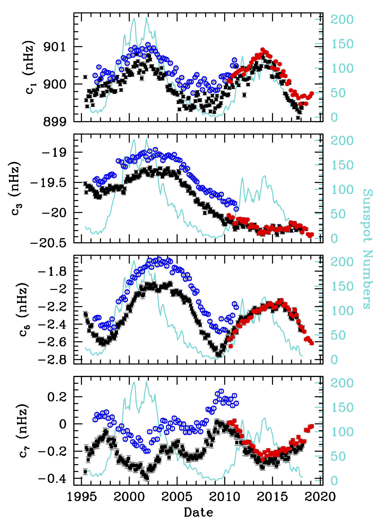
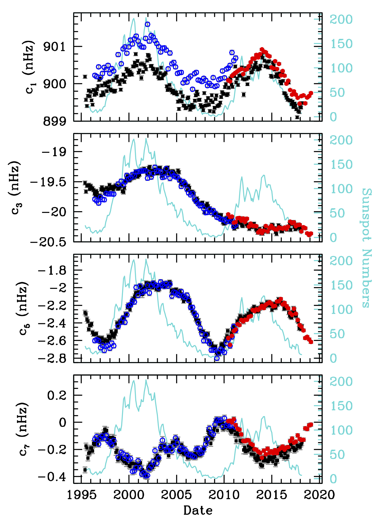
Figure 1: The change of splitting coefficients as a function of time. The points represent averaged splitting coefficients (from top to bottom: $c_{1}$, $c_{3}$, $c_{5}$ and $c_{7}$) for modes with lower turning points between 0.95R_⊙and 0.975R_⊙. The black points are GONG data, blue MDI and red HMI. The column on the left are average of all data, while in the right-hand column we have restricted MDI data to modes with degree $l<120$. In all panels, the cyan lines show SSN values averaged over time intervals that correspond to the GONG sets as the light blue line, with the values on the right-hand axis.

The solar rotation rate is obtained by inverting the odd-order splitting coefficients (Schou et al., 1998), however, the time-variations can be seen easily in the splittings themselves. In the left-hand column of Fig. 1 we show the first four odd-order splitting coefficients averaged over all modes that have lower-turning points between 0.950R_⊙ and 0.975R_⊙. A number of features are clear immediately. First, there are clear systematic differences between MDI and GONG data, much less so between HMI and GONG data. However, the systematic differences are smaller when MDI data are restricted to modes with $l<120$, as can be seen in the right-hand panel of Fig. 1. The problem with high-degree MDI modes were reported earlier by Antia & Basu (2004) and Antia et al. (2008), and it appears that reprocessing by Larson & Schou (2015) has not fully resolved that. A part of the remaining difference between MDI and GONG, particularly for $c_{1}$ is because of the f modes in the MDI data. Similarly, some of the differences between GONG and HMI are because GONG data are restricted to $l<=150$, and because of f modes that are not present in the GONG sets.

It is known that there are systematic differences between GONG and MDI data for rotational splittings (Schou et al., 2002) which yields a slightly different rotation profiles for the two data sets. This differences persist even if $l>120$ modes are neglected. Most of these systematic differences are believed to be due to the difference in processing pipeline (Schou et al., 2002) and are independent of time. As a result, the zonal flows obtained by subtracting the temporal average are not affected significantly by these differences. However, some differences do show up in the gradients of zonal flows (Antia et al., 2008), particularly in near surface layers. These differences can be reduced if $l>120$ modes are neglected as pointed out by Antia et al. (2008). All results shown in this work are obtained by neglecting $l>120$ modes for MDI.

Table 1: Correlation coefficient of splitting coefficients with 10.7 cm radio flux

Coefficient	Both	Cycle 23			Cycle 24
	Cycles	Full	Ascending	Descending	Full	Ascending	Descending
$c_{1}$	$\phantom{-}0.79$	$\phantom{-}0.87$	$\phantom{-}0.83$	$\phantom{-}0.92$	$\phantom{-}0.82$	$\phantom{-}0.77$	$\phantom{-}0.90$
$c_{3}$	$\phantom{-}0.36$	$\phantom{-}0.72$	$\phantom{-}0.84$	$\phantom{-}0.75$	$-0.50$	$-0.72$	$-0.34$
$c_{5}$	$\phantom{-}0.64$	$\phantom{-}0.63$	$\phantom{-}0.91$	$\phantom{-}0.71$	$\phantom{-}0.64$	$\phantom{-}0.88$	$\phantom{-}0.67$
$c_{7}$	$-0.71$	$-0.79$	$-0.93$	$-0.62$	$-0.68$	$-0.87$	$-0.84$

The more interesting features as they relate to the Sun however, are the time variations. For modes that sample this radius range, the $c_{1}$ coefficient appears to change with solar cycle and are largest at the maximum of the cycle; $c_{5}$ has a similar behavior. Coefficient $c_{3}$ however, does not show such a dependence on the 11-year Schwabe cycle, and its time dependence, positive correlation with solar activity indices in Cycle 23 and negative in Cycle 24, makes it tempting to speculate whether it follows a cycle with a longer time scale or shows a more complicated variation. The behavior of the coefficients during Cycle 25 should clarify this. Coefficient $c_{7}$ has a more complicated time variation; in Cycle 24 the coefficient is anticorrelated with solar activity, in Cycle 23 there is a hump-like feature around 2005; since the feature is seen both by GONG and MDI it must be a feature of the Sun and not an instrumental effect.

A correlation analysis of the coefficients with the 10.7 cm flux (Table 1) shows that for the modes shown in the figures, $c_{1}$ is positively correlated with the 10.7 cm flux in both cycles with the correlation coefficient being as high as $0.9$ in the descending phases of the two cycles. Coefficient $c_{5}$ is also positively correlated, but more so in the ascending phases of the two cycles, Additionally, $c_{5}$ seems to show the sharpest change as a new cycle begins — at the start of both Cycle 23 and Cycle 24, $c_{5}$ reversed its fall abruptly and started increasing; in contrast, the change in $c_{1}$ was gentler. Extrapolating the curve for $c_{5}$ it appears that some time in early 2020 it will reach the level that was reached at the minimum around 2009. This could be the time for next solar activity minimum though there is some ambiguity in this criterion.

Note that after solar maximum, there is a noticeable time-lag between the fall of the radio flux and $c_{5}$, this is unlike the case of $c_{1}$, which starts falling as soon as the radio flux does. The coefficient $c_{7}$ shows a more complicated behavior during Cycle 23 with strong negative correlation with the 10.7 cm flux during the ascending part of the cycle, which becomes weaker during the descending part of Cycle 23 possibly because of the feature around 2005. Just like $c_{5}$, $c_{7}$ changes quite abruptly at the onset of the new cycle, with the splittings decreasing. The onset of Cycle 25 should be able to confirm if the abrupt changes in $c_{5}$ and $c_{7}$ are persistent features of all solar cycles.

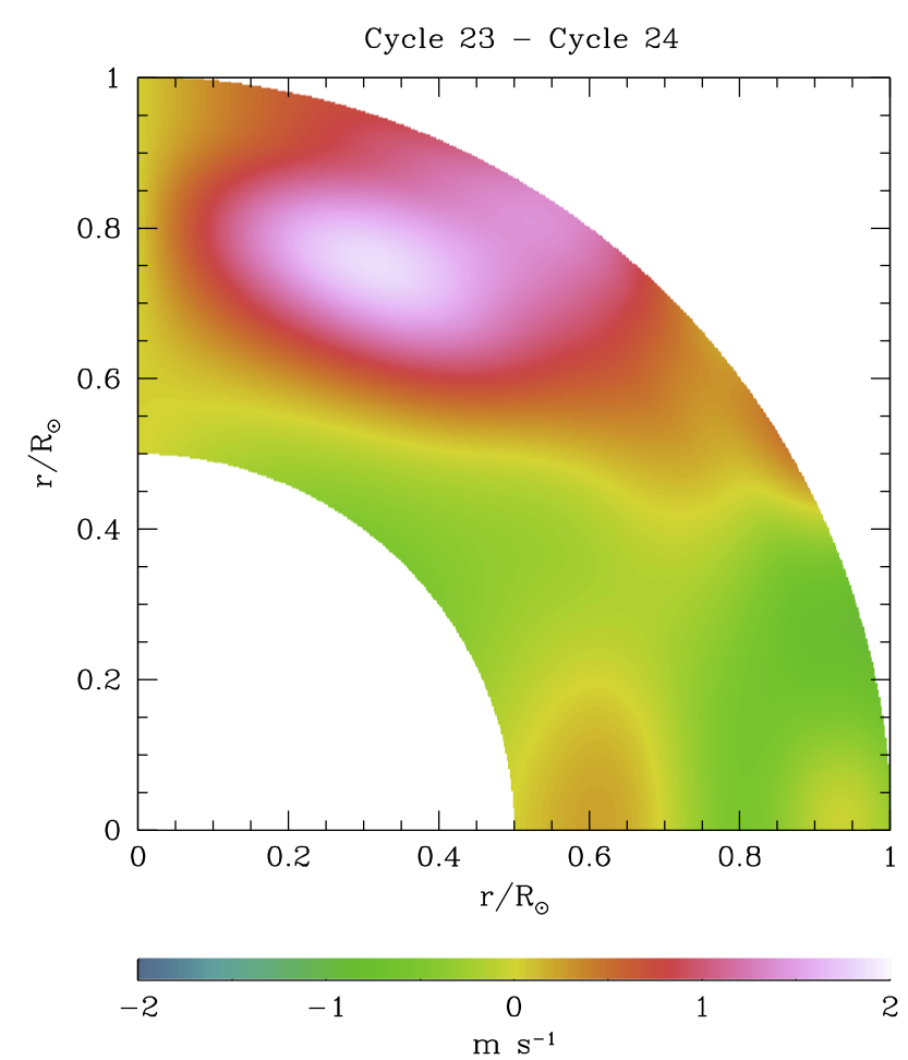
Figure 2: The difference between the average rotational velocities during solar Cycle 23 and solar Cycle  24. The differences are in the sense (Cycle 23 $-$ Cycle 24). Results are for GONG data.

The differences in the time-variations of the splitting coefficients imply that the average rotation rate during Cycle 23 was different from that of Cycle 24, and that the differences will be latitude-dependent, which is indeed the case as shown in Fig. 2. As expected, there are significant differences; in the convection zone, Cycle 23 had lower rotation velocities at the active latitudes but higher velocities at higher latitudes compared with Cycle 24. It should be noted that the differences between the average rotation rates are smaller than the difference in the rotation rate between the minima before Cycle 23 and Cycle 24 (Antia & Basu, 2010), but these results, as we shall see in the next section, have important implications for solar zonal-flows.

4 Zonal flows and their gradients

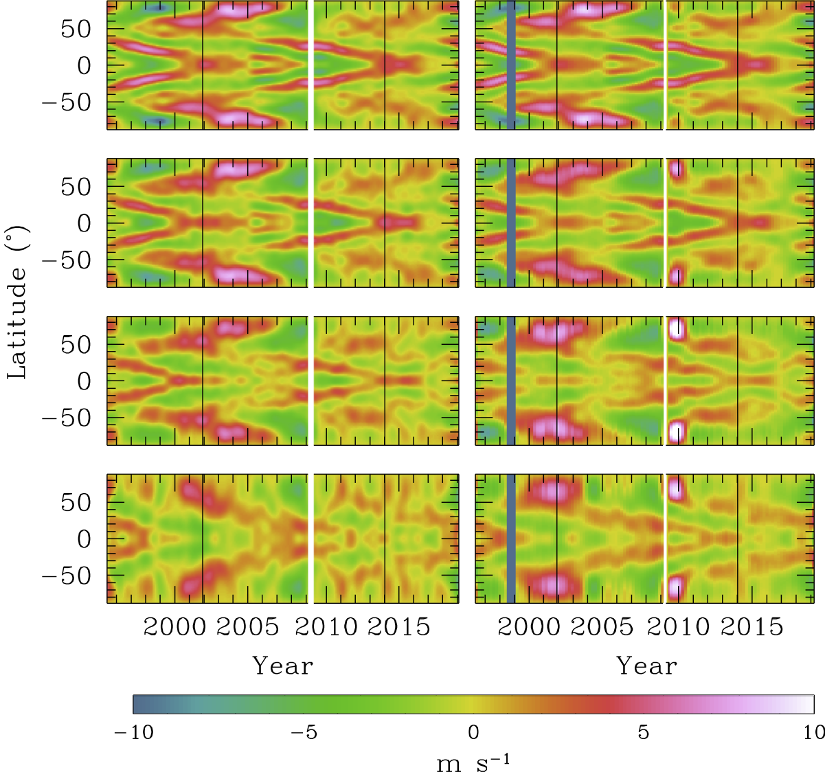
Figure 3: Zonal flow velocities plotted as a function of time and latitude at, from top to bottom, radii of 0.98, 0.95, 0.90 and 0.80R_⊙. GONG results are shown in the left column, and MDI and HMI results in the right column, In both columns, the thin white vertical patch demarcates Cycle 23 and 24. The blue-green vertical patch in the right column covers the time when MDI data were not available because the SOHO spacecraft was out of contact. The two black vertical lines in each panel mark the time of maximum solar activity. The results have been smoothed over a year to reduce the fluctuations that are present in the data sets. The uncertainties in the velocities at low latitudes is about 0.2 m s^-1 at 0.98R_⊙and increases to 0.4 m s^-1 at 0.8R_⊙.

4.1 The analysis

Zonal flows are east-west flows in the Sun with alternating bands of prograde and retrograde flows. Surface observations showed that bands in the active latitudes migrate towards the equator, while higher-latitude bands migrate towards the poles with time (Howard & Labonte, 1980; Ulrich, 2001). These flows are present below the surface too (first seen in f modes, Kosovichev & Schou 1997), and these too migrate to different latitudes with time (Schou, 1999).

Helioseismic studies of zonal flows define them to be residuals left at any epoch when the average rotation velocity is subtracted out, i.e.,

$$\delta v_{\phi}=v_{\phi}(r,\theta,t)-\langle v_{\phi}(r,\theta,t)\rangle,$$ (2)

where $v_{\phi}(r,\theta,t)\equiv\Omega(r,\theta,t)r\cos\theta$ is the rotation velocity at a given position and time in the Sun, and the angular brackets represent the time-average. Here, $\theta$ is the latitude. As is clear from Eq. 2, the results depend on the time over which the averaging is done and hence the weaker features are not very robust. If the average over all data are used, the higher rotation rate of Cycle 23 in the high-latitude regions washes out some of the weaker features of the zonal flow during Cycle 24, in particular, one cannot see the high-latitude poleward branch of the zonal flow during Cycle 24 (Antia & Basu, 2013; Howe et al., 2013a, 2018), this had earlier led to speculation that this might mean that Cycle 25 may be delayed (Hill et al., 2011). Consequently, in this work we treat Cycles 23 and 24 separately.

The differences in the zonal flows can be made clearer by analyzing the spatial gradients of the zonal flows. In keeping with Antia et al. (2008), we calculate the gradients of $\delta\Omega$ rather than $\delta v_{\phi}$. The radial gradient is simply $\delta\Omega_{r}\equiv\partial\delta\Omega/\partial r$, and the latitudinal gradient is $\delta\Omega_{\theta}\equiv(1/r)\partial\delta\Omega/\partial|\theta|$. However, in the results shown later these gradients are multiplied by $\cos\theta$ to balance the latitudinal dependence as in the case of zonal flows.

4.2 Results

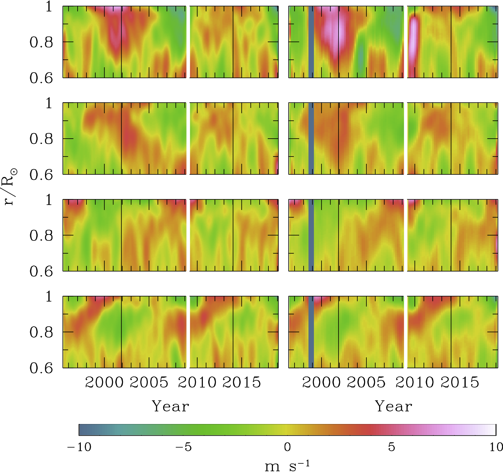
Figure 4: The same as Fig. 3 but plotted a a function of time and radius at, from bottom to top, latitudes of $15^{\circ}$, $30^{\circ}$, $45^{\circ}$ and $60^{\circ}$.

The zonal flow velocities at a few different depths as a function of time and latitude are shown in Fig. 3. If we look at the topmost panels, a few features are clear immediately: despite subtracting a smaller high-latitude average, the poleward flows in Cycle 24 were much weaker than those in Cycle 23. In Cycle 23, the poleward prograde branch end abruptly, and a retrograde band appears in its place close to the end of the cycle; this change is not seen yet for Cycle 24, if anything the prograde band appears to have become stronger. We can also see the beginnings of what will probably be the low-latitude equator-ward branch of the zonal flow of Cycle 25. However, in Cycle 24 we do not see the smaller “tuning fork” type equatorward branch at even lower latitudes, that in Cycle 23 was formed around 2005 just as the main equatorward branch became strong. Thus the changes in the zonal flows between Cycle 23 and 24 are not merely quantitative, but they are qualitatively different as well. It is possible that the higher average active-latitude rotation rate in Cycle 24 is hiding this tuning-fork like feature. Looking deeper, we can see that the high latitude poleward branch is not well defined at $0.8R_{\odot}$. The HMI results for $r=0.90R_{\odot}$ and $0.95R_{\odot}$ also do not show a clear poleward branch at high latitudes, but this could be because the average rotation rate during Cycle 24 is biased by some part of MDI data during the beginning of Cycle 24, which shows up as a prominent feature at high latitudes around 2010. In fact, by artificially moving the start of Cycle 24 at 2010.5 to cut out the MDI contribution the poleward branch shows up just like that in GONG results. The MDI and HMI results show a prominent feature at high latitudes at the beginning of Cycle 24. This is most likely due to systematic differences between the MDI and HMI data sets. It should be noted that the first 1.5 years data in Cycle 24 is from MDI and the rest from HMI. This feature is also seen at $60^{\circ}$ latitude in Fig. 4.

In Fig. 4 we show the zonal flow velocities as a function of radius at different latitudes. As can be seen, the radial pattern of the zonal flows is qualitatively similar at low latitudes in both cycles, with prograde bands rising from deep inside the convection zone to the surface as a function of time. At the edge of the active latitudes ($30^{\circ}$, second row from bottom) a rising band is seen which starts rising from the convection-zone base just about the same time as the equatorial prograde flow reaches the solar surface, just before solar maximum, and straddles the solar minimum. Thus in a sense, this $30^{\circ}$ prograde band is precursor of the next cycle. Although this flow is less clear in Cycle 24, it is still visible showing the beginnings of Cycle 25. Above the active latitudes, and we have shown the results at $45^{\circ}$, the solar maximum marks the “sinking” of the prograde flow. This band appears less well-defined in Cycle 24 than in Cycle 23.

Also of interest are the spatial gradients of the zonal flows, we show those in Fig. 5. On examining the latitudinal gradient of the zonal flow rate, it is clear that the gradients were stronger and more well defined in Cycle 23 than in Cycle 24. This is particularly true for the high-latitude band. The high-latitude band shows an abrupt change from positive to negative close to the end of Cycle 23, we do not see such a change in the Cycle 24 data, most likely indicating that we are not close to the end of Cycle 24. The minimum after Cycle 23 occurred about one year after the change of sign of the high-latitude gradient. If that feature is an indicator of a shift in activity, we are not close to the minimum after Cycle 24. Indeed, Upton & Hathaway (2018) using different indicators claim that Cycle 24 will end closer to the end of 2020 or in early 2021. The radial gradients are more confusing as can be seen in the right-hand panel of Fig. 5. The high-latitude results obtained with MDI and HMI data do not agree with those obtained with GONG data, however, the results for the active latitudes do agree. Again, Cycle 23 had larger gradients (both positive and negative) than Cycle 24. And as had been seen for Cycle 23 by Antia et al. (2008), sunspots appear where the the gradients of the zonal flow are large. A closer examination of both cycles show that sunspots appear in the low-latitude regions that have a large negative latitudinal gradient and a large positive radial gradient.

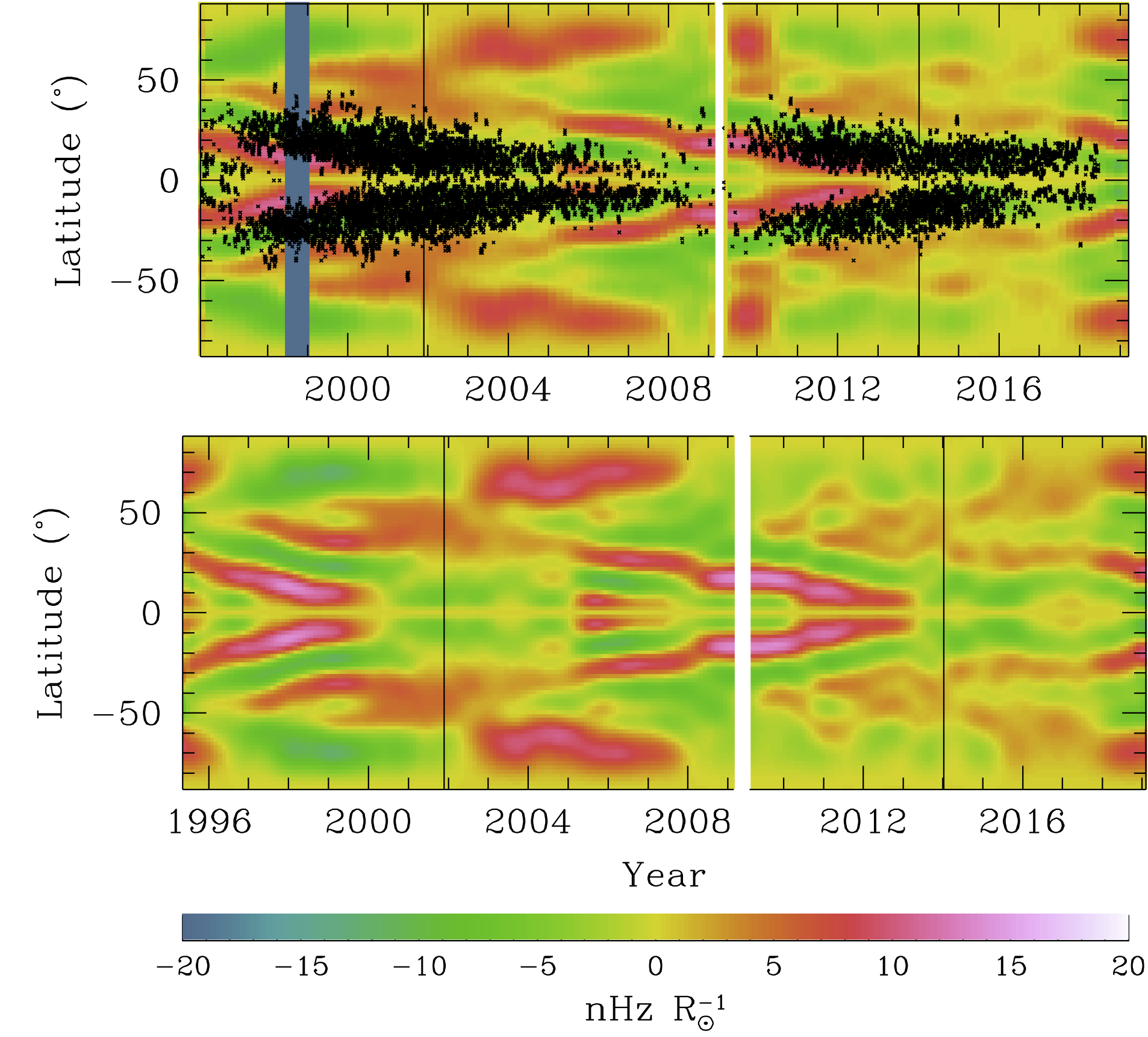
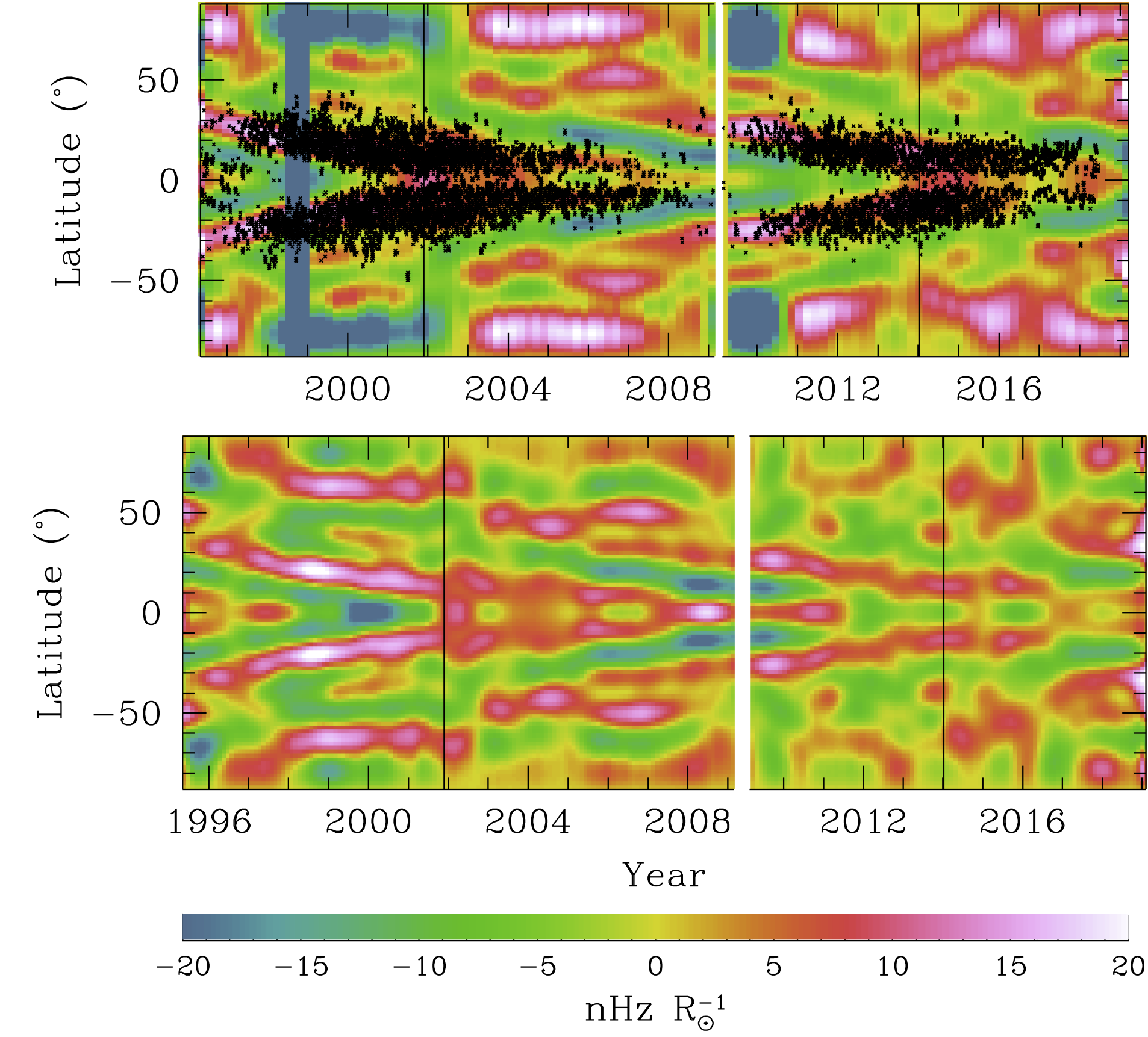
Figure 5: Left column: The latitudinal gradient, $(1/r)(\partial\delta\Omega/\partial|\theta|)\cos\theta$ of the zonal flow rate at 0.95R_⊙. Right column: The radial gradient, $(\partial\delta\Omega/\partial r)\cos\theta$ of the zonal flow rate at 0.95R_⊙. In both columns, the upper panels are results from MDI and HMI, the lower panel shows results from GONG. The position of sunspots are marked in the upper panel.

5 The tachocline

5.1 The analysis technique

The tachocline is too thin to be resolved with the usual inversion techniques (Kosovichev, 1996; Schou et al., 1998; Antia et al., 1998), consequently like in earlier works (Antia et al., 1998; Antia & Basu, 2011) we use a forward modelling technique to model the tachocline at each epoch to determine the properties and their time-variations. This therefore involves adopting a model of the tachocline, determining the splitting coefficients for different free parameters of the tachocline and comparing the model coefficients with the observed ones to find the set of parameters that give the lowest mismatch with the observations, as quantified by the value of $\chi^{2}$. We use splittings of all modes with lower turning points between $0.5R_{\odot}$ and $0.9R_{\odot}$. The lower limit is imposed because of increased uncertainty of the splittings of modes that probe deeper; the upper limit is set so that the signature of the near-surface shear layer does not dominate the signal of the splitting coefficients.

We use the method of simulated annealing (Vanderbilt & Louie, 1984; Press et al., 1992) to minimize $\chi^{2}$. The algorithm uses randomly generated values of the parameters, and we assume that the parameters have Gaussian priors with the mean and width of the Gaussian determined from inversions of rotational splittings. While inversions do not resolve the tachocline very well, they do define it. Since the tachocline has many parameters, there is the likelihood of the solution being trapped in a local minimum; to avoid this, we make 80 attempts using different sequences of random numbers in the annealing procedure to find the global $\chi^{2}$ minimum. We determine the uncertainties using a traditional boot-strapping method where we simulated many realizations of the observations, fit each one of them in exactly the same manner as the original data and use the spread as a measure of uncertainty.

5.2 The tachocline model

We consider both one-dimensional and two dimensional models for the tachocline. As in our earlier work (Basu, 1997; Antia et al., 1998; Antia & Basu, 2011), we model the tachocline as

$$\Omega_{\rm tach}=\frac{\Delta\Omega}{1+\exp[(r_{d}-r)/w]},$$ (3)

where $r$ is radius, $r_{d}$ the mean position of the tachocline, $\Delta\Omega$ the jump in rotation rate between radii $r$ where $r<r_{d}$ and $r>r_{d}$, and $w$ the width such that the rotation rate changes from a factor $1/(1+e)$ of the maximum to a factor $e/(1+e)$ in the range $r=r_{d}-w$ and $r=r_{d}+w$. The same model can be applied in a latitude dependent manner with $\Delta\Omega$, $r_{d}$ and $w$ made functions of co-latitude (Antia et al., 1998; Antia & Basu, 2011).

Another model that has been used in literature (Kosovichev, 1996; Charbonneau et al., 1999) is

$$\Omega_{\rm tach}={\Delta\Omega}\frac{1}{2}{\left(1+\mbox{erf}\left[\frac{2(r-r_{d})}{w}\right]\right)},$$ (4)

where $w$, the width is now the radial extent over which 0.84 of the full transition in the rotation rate takes place, i.e., a change from 0.08 to 0.92 of $\Delta\Omega$, this is different from our model, where the width is defined as half the width over which $\Delta\Omega$ changes from 0.269 to 0.731 of its value. Thus when we fit Eq. 4 to the data, we would expect the value of $w$ to be different but related to the width that we define in our model. The two functions have similar shape, but the width in this model is about 5 times that in the model in Eq. 3. We have tried this model too, and aside from the scaling of width there is no significant difference in the fitted parameters.

The tachocline has both a radial and a latitudinal dependence, in particular, the change in rotation rate, i.e., the jump, across the tachocline is strongly dependent on latitude. An added complication is that the rotation rate of the Sun in regions away from the tachocline can have radial gradients. We choose a 2D model that is similar to our earlier works (Antia & Basu, 2011):

$$\Omega(r,\vartheta)=\begin{cases}{\Omega_{c}+\frac{\Delta\Omega}{1+\exp[(r_{d}-r)/w]}}&\mbox{if }r\leq 0.7R_{\odot}\\ \Omega_{c}+B(r-0.7)+{\Delta\Omega\over{1+\exp[(r_{d}-r)/w]}}&\mbox{if }0.7<r\leq 0.95R_{\odot}\\ \Omega_{c}+0.25B-C(r-0.95)+{\Delta\Omega\over{1+\exp[(r_{d}-r)/w]}}&\mbox{if }r>0.95R_{\odot}\end{cases}$$ (5)

Where, $\Omega_{c}$, $B$, $C$ are the three parameters defining the smooth part of rotation rate while as usual $\Delta\Omega$, $r_{d}$ and $w$ define the tachocline. Here $B$ defines the gradient in deep convection zone, while $C$ is the gradient in the near surface shear layer. Note that the coefficients $B$ and $C$ are fitted for each epoch and thus can be time dependent.

The co-latitude dependence of the different parameters are:

$$\Delta\Omega= \Delta\Omega_{3}P_{3}(\vartheta)+\Delta\Omega_{5}P_{5}(\vartheta),$$ (6)

$$r_{d}= r_{d1}+r_{d3}P_{3}(\vartheta),$$ (7)

$$w= w_{1}+w_{3}P_{3}(\vartheta),$$ (8)

where using the definition of splitting coefficients (cf., Ritzwoller & Lavely, 1991)

$$P_{3}(\vartheta) =5\cos^{2}\vartheta-1,$$ (9)

$$P_{5}(\vartheta) =21\cos^{4}\vartheta-14\cos^{2}\vartheta+1,$$ (10)

and $\vartheta$ is the co-latitude. The difference between this model and the earlier ones lie in the definition of $B$, in this model $B$ does not have a latitudinal variation, while in the earlier work $B$ was defined as $B=B_{1}+B_{3}P_{3}(\vartheta)+B_{5}P_{5}(\vartheta)$. More importantly in our current model, $\Delta\Omega$ does not have latitude-independent term $\Delta\Omega_{1}$. These changes were made because we found that the marginalized probability distribution functions of these quantities were rather flat. Omitting these parameters helped stabilize the fits for the other quantities. It should be noted that $\Delta\Omega$ represents the variation in $\Omega$ in region near the tachocline and is not affected by rotation rate near the surface which would be reflected in the smooth part of $\Omega$ modeled by parameters $B$ and $C$.

5.3 Results

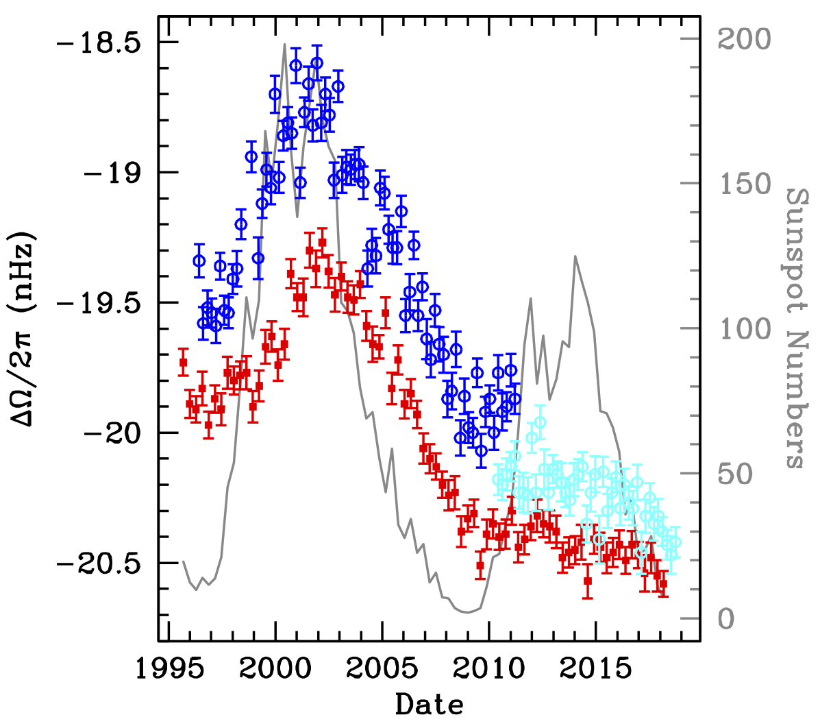
Figure 6: The variation of the change in rotation rate across the tachocline as a function of time as seen in splitting coefficient $c_{3}$. Red points are results obtained using GONG data, deep blue with MDI data and cyan with HMI data. The systematic difference between MDI and GONG results can be reduced to the HMI-GONG level by restricting the MDI modes to $l<120$ as mentioned in Section 3. The gray curve in the background is the sunspot number that can be read from the scale of the ordinate on the right hand side of the box.

In keeping with earlier work, we first fitted the $c_{3}$ coefficient, which shows the largest signal of the tachocline, alone to the model in Eq. 3. Although, the $c_{3}$ results in Fig 1 are for a much shallower radius, the change in $c_{3}$ with time leads us to expect a variation in tachocline properties with time. The results of $\Delta\Omega$, the jump across the tachocline are shown in Fig. 6. Clearly, the quantity shows a statistically significant time variation. Also note that while in Cycle 23 $\Delta\Omega$ shows a variation that reflects the change in solar activity indices, the change is much more subtle in Cycle 24. Also note that although there is a small systematic difference between the GONG and MDI+HMI results, the time variations remain the same. In contrast to $\Delta\Omega$, the position and width of the tachocline shows no discernible change with time, as is shown in Fig. 7, and and in particular, we do not see any significant “pulsations” in the tachocline position as has been hypothesized (de Jager et al., 2016). The results do not change if we use the tachocline model in Eq. 4 instead of Eq. 3.

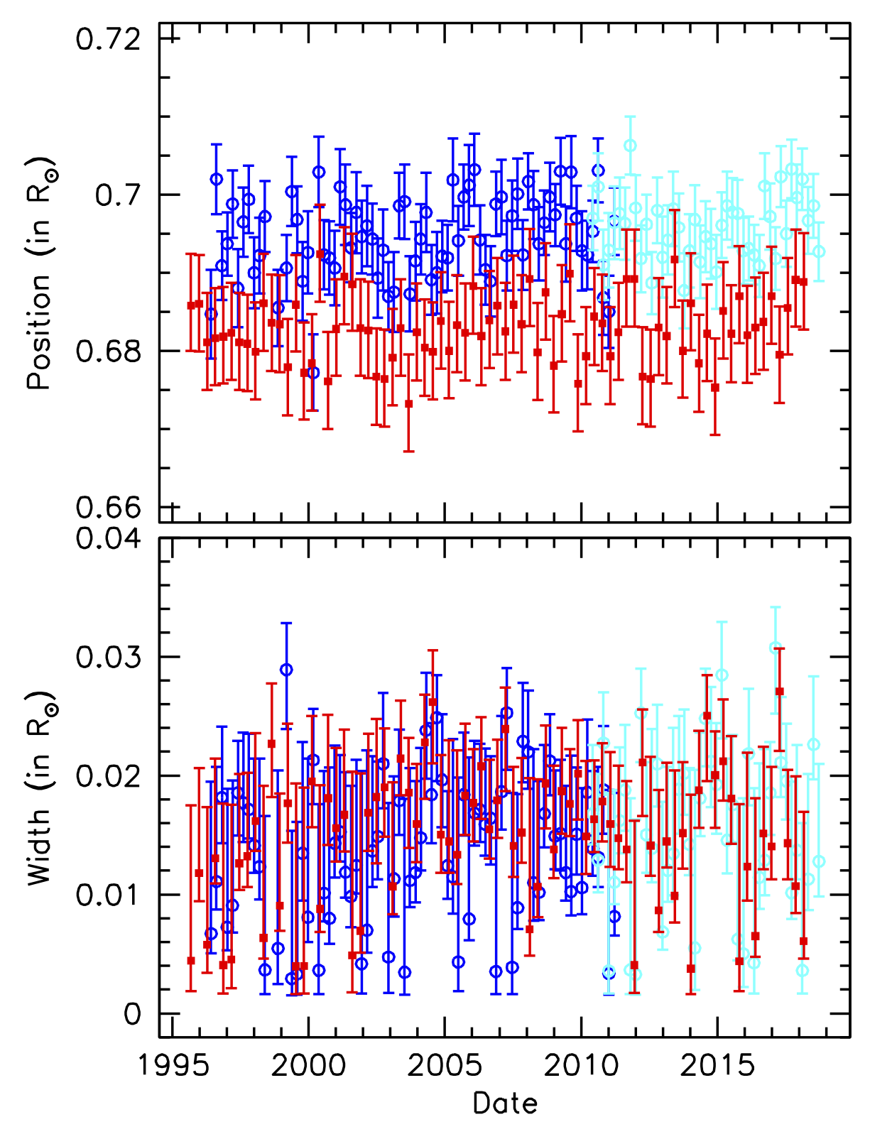
Figure 7: The variation of the position and width of the tachocline as determined from splitting coefficient $c_{3}$. Red points are results obtained using GONG data, deep blue with MDI data and cyan with HMI data.

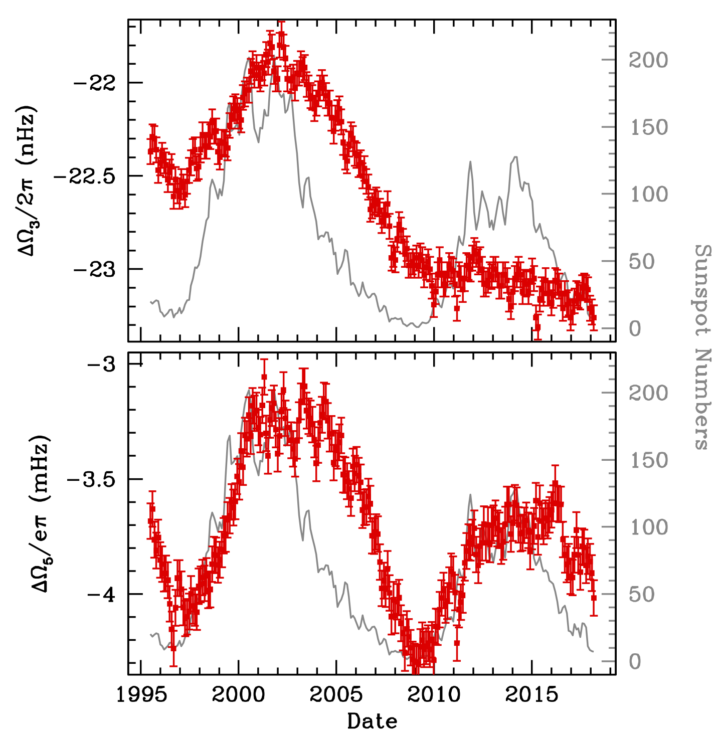
Figure 8: The two components of the jump across the tachocline $\Delta\Omega_{3}$ and $\Delta\Omega_{5}$ plotted as a function of time. Only GONG results are shown. The gray line in the background is the SSN plotted on the scale to the right of the panels.

The $\Delta\Omega_{3}$ and $\Delta\Omega_{5}$ parameters obtained by fitting the two-dimensional model (i.e., fitting Eq. 5) are shown in Fig. 8. We can see that $\Delta\Omega_{3}$ is basically unchanged from that shown in Fig. 6 where we fitted a much simpler model only to $c_{3}$. This shows that the results are robust. We find that the two components of the jump across the tachocline follow the time variation of the coefficients shown in Fig. 1, i.e., $\Delta\Omega_{5}$ follows the sunspot number, while $\Delta\Omega_{3}$ does, not. Since $\Delta\Omega_{3}$ and $\Delta\Omega_{5}$ determine the latitudinal behavior of the jump, we expect the different latitudes to behave quite differently in the two cycles. This is indeed the case, as is shown in Fig. 9. We only show the results for $\Delta\Omega$ since like earlier $r_{d}$ and $w$ do not show any significant time variation. Note that at no latitude does the time variation of $\Delta\Omega$ during Cycle 24 look like the variation in Cycle 23. If there were a one-to-one relation between solar activity and the properties of the tachocline, we would have expected Cycle 24 results to be a repeat of the Cycle 23 results, but with a smaller change between solar maximum and minimum in keeping with the overall lower activity level of Cycle 24; instead we see that low and intermediate latitudes, the nature of the change is completely different. The results are also plotted against the 10.7 cm flux, and it is clear that at the same level of activity, the jump of the rotation rate across the tachocline was very different.

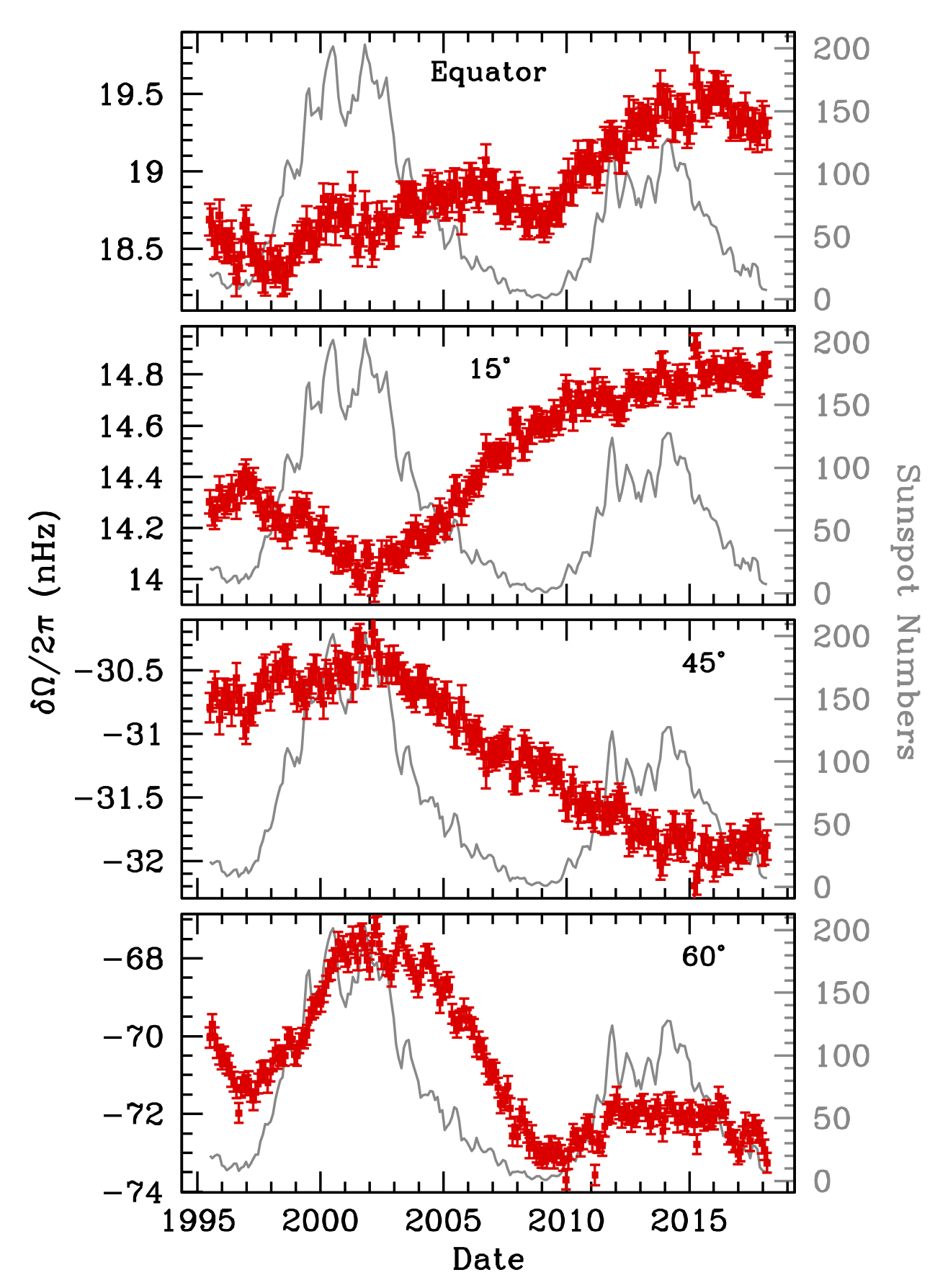
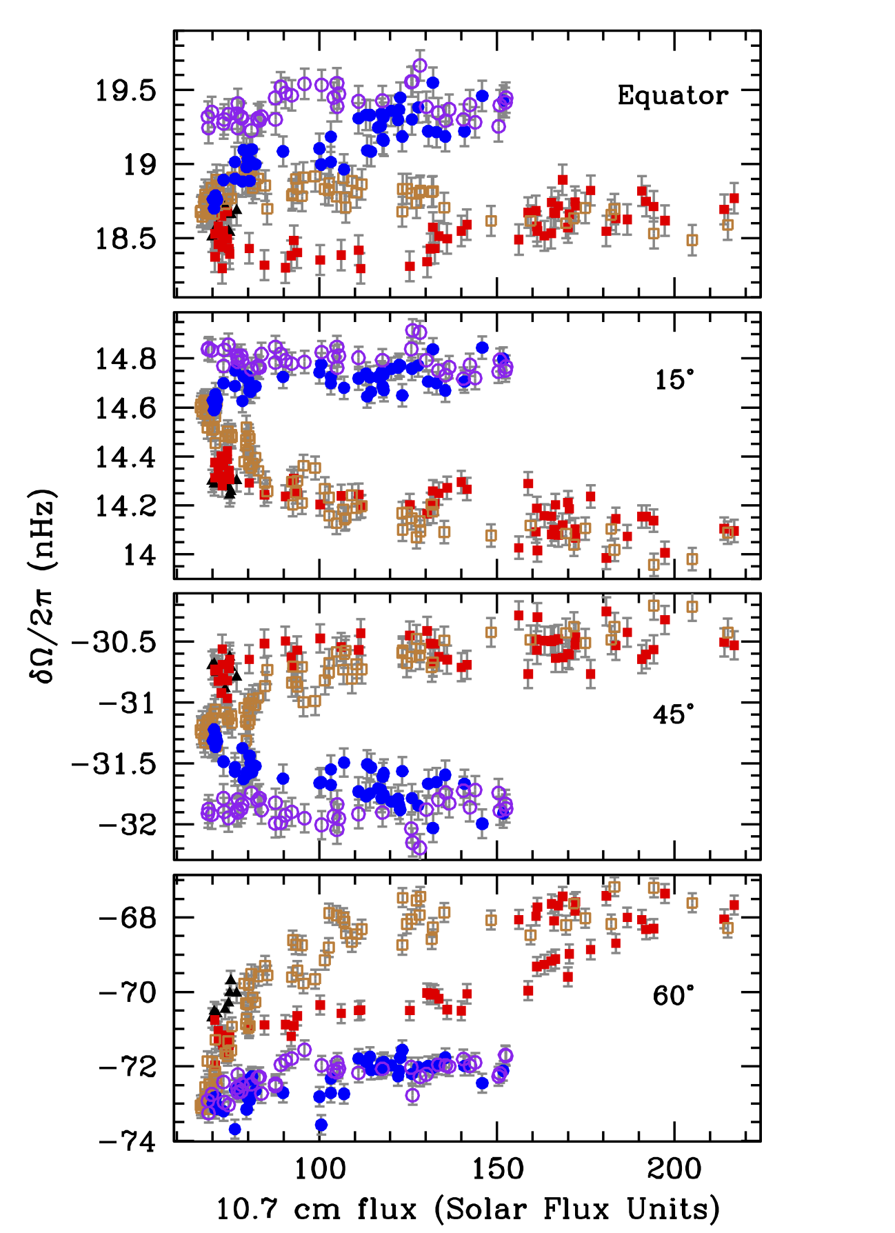
Figure 9: Left: The change in the tachocline with time at different latitudes is shown by red points. Only GONG results have been shown for clarity. The gray curve in the background is the SSN that can be read from the scale of the ordinate on the right hand side of the panels. Right: The change in the tachocline as a function of the flux of 10.7 cm radio emission, which is a proxy for solar activity. In each panel, the black triangles mark the descending phase of Cycle 22, red filled squares the ascending phase of Cycle 23, brown open square show the descending phase of Cycle 23, blue filled circles and purple open squares are respectively the ascending and descending phases of Cycle 24. Only GONG results are shown. The flux is in Solar Flux Units (SFU), with 1 SFU $=10^{4}$ Jansky $=10^{-22}$ W m^-2 Hz^-1.

The change in the rotation rate across the tachocline can actually be plotted the way we have plotted the zonal flows, by subtracting out the average jump over each cycle at each latitude. This is shown in Fig: 10, it should be noted that unlike zonal flow figures, the results at different latitudes are at different radii, the radius at each latitude is $r_{d}$ obtained from the fits to Eq. 5. Subtracting the average jump over each cycle shows that the time-variation during each cycle is more similar, however a few features stand out immediately: (1) there are alternating bands of positive and negative change, and the behavior in time is latitude dependent. (2) At the solar maximum, the behavior of the tachocline above active latitudes is much more marked in Cycle 23 than that at the maximum of Cycle 24. (3) At the start of each cycle, there is a positive band in the mid-latitude regions, that in Cycle 24 reaches to higher latitudes than in Cycle 23; the band is also somewhat stronger in Cycle 24. (4) The mid-latitude negative band is stronger in Cycle 23 than in Cycle 24. (5) The two intense high-latitude negative region in Cycle 23 are barely noticeable in Cycle 24. Since Figure 10 shows residuals when the average jump over each cycle is subtracted out, there is little contribution in Cycle 24 from the splitting coefficient $c_{3}$ which is almost constant during this period. As a result, the contribution from coefficient $c_{5}$ dominates. During cycle 23 on the other hand, the major contribution is from the coefficient $c_{3}$. Thus while the qualitative differences in the nature of the tachocline between the two cycles remain, though in this form that are not as dramatic as the changes shown in Figure 9.

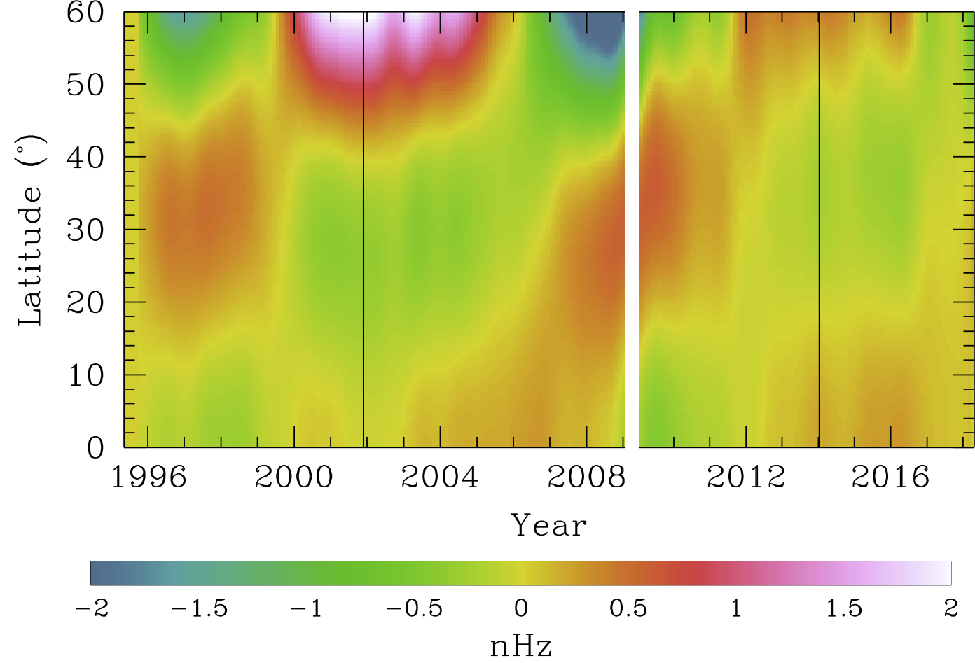
Figure 10: The change in the jump across the tachocline plotted as a function of time and latitude. In order to show the change clearly, the average value of jump during each solar cycle has been subtracted from the value at each latitude. The blank space demarcates the two cycles. This way of plotting emphasizes the behavior with time, rather than the overall magnitude of the tachocline, which as shown in Fig. 9, differed in the two solar cycles.

6 Summary and Conclusions

Our analysis of solar rotation using helioseismic data has revealed some surprises. If we confine our attention to oscillation modes that have lower turning points in the outer convection zone, we find that splitting coefficient $c_{3}$ has behaved very different from the others; it does not show a monotonic change in activity and instead has kept decreasing since the maximum of Cycle 23. Changes in $c_{3}$ in the upcoming Cycle 25 should tell us if $c_{3}$ varies periodically at all. Coefficients $c_{5}$ and $c_{7}$ show an abrupt change at the beginning of solar Cycles 23 and 24, and again Cycle 25 will reveal whether these can be used as a marker of the onset of the solar cycle.

The average solar rotation rate over Cycle 23 was quite different than the average over the current span of Cycle 24. Cycle 23 had higher rotation velocities at high latitudes, but lower at the low latitudes. The difference in the average rotation rate affects the zonal flow pattern that is seen in the two cycles. As a result, to see the zonal flows clearly, particularly during Cycle 24 we subtract separate averages over each cycle. The fact that the zonal flow pattern and velocities depend on the average subtracted is an indication of the fact that the way zonal flows are revealed is not robust and the subtraction of an incompatible average can yield misleading results. Note that some of the differences could be due to the fact that Cycle 24 has not ended yet.

The zonal flow pattern in Cycle 24 was much less defined, and had lower velocities than Cycle 23. In particular, the high-latitude poleward branch is very weak. Our results confirm those of Howe et al. (2018). Like Howe et al. (2018) we see the start of the dynamical effects of solar Cycle 25. The signs are clearer when the flows are examined as a function of radius at a latitude of about $30^{\circ}$. In Cycle 23, a prograde branch appeared after the maximum at this latitude near the tachocline and that rose up to form the low-latitude prograde flow in Cycle 24; we see that such a band did form after the Cycle 24 maximum too. The band is however, quite weak, leading us to believe that Cycle 25 will be quite weak.

The spatial gradients of the zonal flows in Cycle 23 and 24 show that sunspots are formed where and when a large negative latitudinal gradient and a large positive radial gradient arise at low latitudes in near surface layers. However, these gradients are different for the two cycles. We are yet to see a change in the sign of the latitudinal gradient of the poleward branch; Cycle 23 ended about a year after that shift, and its absence in Cycle 24 so far leads us to believe that Cycle 25 is not imminent, unlike the prediction of Howe et al. (2018), but could be delayed as predicted by Upton & Hathaway (2018).

The dynamics of the tachocline were very different in the two solar cycles. While we did not find any statistically significant changes in the position or width of the tachocline, we find that the change in rotation rate across the tachocline had a different variation in Cycle 23 compared with Cycle 24. The changes cannot be explained as just a dependence on solar activity — the jump in rotation, $\Delta\Omega$ is different in the two cycles for the same value of the sunspot number or the 10.7 cm flux. This is mainly a result of the time variation of splitting coefficient $c_{3}$, the one with the largest signature of the tachocline; the jump in tachocline resulting from the splitting coefficient $c_{5}$ shows similar behavior in the two cycles and basically follows the the solar activity indices, albeit with a small delay at the descending phase.

References

- Antia & Basu (2000) Antia, H. M., & Basu, S. 2000, ApJ, 541, 442
- Antia & Basu (2001) —. 2001, ApJ, 559, L67
- Antia & Basu (2004) Antia, H. M., & Basu, S. 2004, in ESA Special Publication, Vol. 559, SOHO 14 Helio- and Asteroseismology: Towards a Golden Future, ed. D. Danesy, 301
- Antia & Basu (2010) —. 2010, ApJ, 720, 494
- Antia & Basu (2011) —. 2011, ApJ, 735, L45
- Antia & Basu (2013) Antia, H. M., & Basu, S. 2013, in Journal of Physics Conference Series, Vol. 440, Journal of Physics Conference Series, 012018
- Antia et al. (1998) Antia, H. M., Basu, S., & Chitre, S. M. 1998, MNRAS, 298, 543
- Antia et al. (2008) —. 2008, ApJ, 681, 680
- Baranyi et al. (2016) Baranyi, T., Győri, L., & Ludmány, A. 2016, Sol. Phys., 291, 3081
- Basu (1997) Basu, S. 1997, MNRAS, 288, 572
- Basu et al. (2012) Basu, S., Broomhall, A.-M., Chaplin, W. J., & Elsworth, Y. 2012, Astrophys. J., 758, 43
- Charbonneau et al. (1999) Charbonneau, P., Christensen-Dalsgaard, J., Henning, R., et al. 1999, ApJ, 527, 445
- de Jager et al. (2016) de Jager, C., Akasofu, S.-I., Duhau, S., et al. 2016, Space Sci. Rev., 201, 109
- Gilman (2005) Gilman, P. A. 2005, Astronomische Nachrichten, 326, 208
- Győri et al. (2017) Győri, L., Ludmány, A., & Baranyi, T. 2017, MNRAS, 465, 1259
- Hill et al. (2011) Hill, F., Howe, R., Komm, R., et al. 2011, in IAU Symposium, Vol. 271, Astrophysical Dynamics: From Stars to Galaxies, ed. N. H. Brummell, A. S. Brun, M. S. Miesch, & Y. Ponty, 15–22
- Hill et al. (1996) Hill, F., Stark, P. B., Stebbins, R. T., et al. 1996, Science, 272, 1292
- Howard & Labonte (1980) Howard, R., & Labonte, B. J. 1980, ApJ, 239, L33
- Howe et al. (2013a) Howe, R., Christensen-Dalsgaard, J., Hill, F., et al. 2013a, ApJ, 767, L20
- Howe et al. (2013b) Howe, R., Christensen-Dalsgaard, J., Hill, F., et al. 2013b, in Astronomical Society of the Pacific Conference Series, Vol. 478, Fifty Years of Seismology of the Sun and Stars, ed. K. Jain, S. C. Tripathy, F. Hill, J. W. Leibacher, & A. A. Pevtsov, 303
- Howe et al. (2000) —. 2000, ApJ, 533, L163
- Howe et al. (2017) Howe, R., Davies, G. R., Chaplin, W. J., et al. 2017, MNRAS, 470, 1935
- Howe et al. (2018) Howe, R., Hill, F., Komm, R., et al. 2018, ApJ, 862, L5
- Komm et al. (2014) Komm, R., Howe, R., González Hernández, I., & Hill, F. 2014, Sol. Phys., 289, 3435
- Kosovichev (1996) Kosovichev, A. G. 1996, ApJ, 469, L61
- Kosovichev & Pipin (2019) Kosovichev, A. G., & Pipin, V. V. 2019, ApJ, 871, L20
- Kosovichev & Schou (1997) Kosovichev, A. G., & Schou, J. 1997, ApJ, 482, L207
- Larson & Schou (2015) Larson, T. P., & Schou, J. 2015, Sol. Phys., 290, 3221
- Larson & Schou (2018) —. 2018, Sol. Phys., 293, 29
- Press et al. (1992) Press, W. H., Teukolsky, S. A., Vetterling, W. T., & Flannery, B. P. 1992, Numerical recipes in FORTRAN. The art of scientific computing (Cambridge: University Press, —c1992, 2nd ed.)
- Ritzwoller & Lavely (1991) Ritzwoller, M. H., & Lavely, E. M. 1991, ApJ, 369, 557
- Scherrer et al. (1995) Scherrer, P. H., Bogart, R. S., Bush, R. I., et al. 1995, Sol. Phys., 162, 129
- Scherrer et al. (2012) Scherrer, P. H., Schou, J., Bush, R. I., et al. 2012, Sol. Phys., 275, 207
- Schou (1999) Schou, J. 1999, ApJ, 523, L181
- Schou et al. (1998) Schou, J., Antia, H. M., Basu, S., et al. 1998, ApJ, 505, 390
- Schou et al. (2002) Schou, J., Howe, R., Basu, S., et al. 2002, ApJ, 567, 1234
- SILSO World Data Center (1995–2019) SILSO World Data Center. 1995–2019, International Sunspot Number Monthly Bulletin and online catalogue
- Tapping (2013) Tapping, K. F. 2013, Space Weather, 11, 394
- Tapping & Morton (2013) Tapping, K. F., & Morton, D. C. 2013, in Journal of Physics Conference Series, Vol. 440, Journal of Physics Conference Series, 012039
- Ulrich (2001) Ulrich, R. K. 2001, ApJ, 560, 466
- Upton & Hathaway (2018) Upton, L. A., & Hathaway, D. H. 2018, Geophys. Res. Lett., 45, 8091
- Vanderbilt & Louie (1984) Vanderbilt, D., & Louie, S. G. 1984, Journal of Computational Physics, 56, 259
- Vorontsov et al. (2002) Vorontsov, S. V., Christensen-Dalsgaard, J., Schou, J., Strakhov, V. N., & Thompson, M. J. 2002, Science, 296, 101