Photon scattering from a cold, Gaussian atom cloud

Abstract

We study the effect of a weakly driven atomic cloud’s polarization distribution on its photon scattering lineshape. In doing this, we find three distinct polarization regimes. First, for dilute clouds, the polarization magnitude is relatively constant. Second, for denser clouds, polarization builds at the front of the cloud for near-resonant light. Third, when the cloud condenses to the point where its dimensions become comparable to the wavelength, light refocuses towards the back of the cloud for red detuning. For these regimes, we show which ‘mean-field’ frameworks accurately describe the differing photon scattering lineshapes. Finally, for even denser clouds, mean field models become inaccurate and necessitate the full point dipole model that includes atom-atom correlations.

I Introduction

Scientists study light-matter interactions with an ostensibly diverse set of physical models. “Microscopic” models—that treat atoms as point dipoles—have been integral to understanding effects such as superradiant spontaneous emission Dicke (1954); Rehler and Eberly (1971); Gross and Haroche (1982); Sutherland and Robicheaux (2017a), coherent scattered radiation Rehler and Eberly (1971); Ruostekoski and Javanainen (1997); Scully et al. (2006); Scully (2007); Sutherland and Robicheaux (2016a, b); Bromley et al. (2016); Bettles et al. (2016); Svidzinsky and Chang (2008); Jenkins and Ruostekoski (2012a); Sutherland and Robicheaux (2017b); Zhu et al. (2016), collective Lamb-shifts Meir et al. (2014), and Anderson localization Anderson (1958); Störzer et al. (2006); Skipetrov and Sokolov (2015). Within the microscopic model, some analyses leverage other mean-field approximations such as assuming an evenly excited phase distribution (timed-Dicke state) Rehler and Eberly (1971); Scully et al. (2006), or using clouds that are denser but have less atoms than the represented cloud Bromley et al. (2016). “Mean-field” approaches—that treat illuminated matter as continuous dielectrics Jackson (1999)—are also an intuitive tool for understanding many of these same effects Mie (1908); Friedberg et al. (1973); Cottier et al. (2018). While there has been recent work towards understanding the relationships between these treatments Javanainen et al. (2014); Javanainen and Ruostekoski (2016); Cottier et al. (2018), where and why models fail to reproduce the results of the full point dipole system remains largely unexplored.

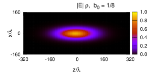
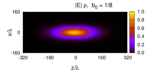
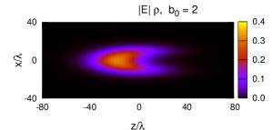
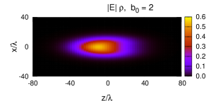
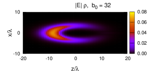
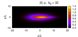
Figure 1: The continuum model calculation for the $y=0$ cross section of the spatial dependence of $|E|\rho$ which is proportional to the polarizability. In all plots, $|E|$ has been divided by $|E|$ at $z\to-\infty$ and the density is divided by the peak density; if there were no attenuation or focusing, the $|E|\rho$ would have a maximum value of 1 at $x=z=0$. In all calculations, the on resonance and on axis optical depths $OD=2b_{0}$. The spatial density is characterized by $\xi=2$, Eq. (1) and $N=2^{11}$. The detuning is set at $\Delta=0$ for the left column and $\Delta=-0.4(1+b_{0}/4)\Gamma$ for the right column to accentuate the focusing effect. The electric field is scaled by the incident field and the density is scaled by the maximum density.

In this work, we compare the continuous dielectric model with the full point dipole calculations of a frozen atomic cloud of two-level atoms driven by a weak laser. In order to do this, we implement a unique iterative numerical technique capable of simulating over $10^{5}$ atoms without approximation. We find three distinctive regimes of the cloud (see Fig. 1), each characterized by its polarization distribution. The figure shows a continuum dielectric calculation of the scaled $|E|\rho$ where $|E|$ is the local magnitude of the electric field and $\rho$ is the average atom density; in the plots, $y=0$ and the light is polarized in the $x$-direction and propagates in the $z$-direction. The left column is for detuning $\Delta=0$ while the right column is for red detuning, $\Delta=-0.4(1+b_{0}/4)\Gamma$. First, for clouds with small optical depths, OD, the atom excitations are nearly evenly distributed throughout the cloud for all laser detunings (see the $b_{0}=1/8$ case); thus, models that assume an even distribution Scully et al. (2006) give good agreement with the full point dipole model. When the cloud becomes more dense, the laser intensity is substantially reduced as it traverses the cloud, causing excitation to be much more likely in the front of the cloud for near-resonant light, causing non-Lorentzian lineshapes; this is exemplified by the $b_{0}=2$ case where $\Delta=0$, left column, has considerable attenuation while the detuned case, right column, has more uniform excitation. We find that, in this regime, our cloud is well described by a continuous dielectric solved using the eikonal approximation in Maxwell’s equations. When the eikonal approximation is valid, the photon scattering is well described by a single parameter, OD. Finally, for clouds with dimensions comparable to a wavelength, the light refocuses towards the back of the cloud for red detuning Sutherland and Robicheaux (2016a) (see the $b_{0}=32$ case); the red detuned light causes larger polarization for $z>0$ through the center of the cloud whereas there is almost no polarization near the center of the cloud for zero detuning, causing the eikonal approximation —and the cloud’s dependence on OD —to break down. For all of the cases in Fig. 1, the continuum dielectric model reproduces the total photon scattering and forward photon scattering rate from point dipole calculations averaged over many spatial configurations, even the $b_{0}=32$ cases although accuracy requires the higher-order paraxial approximation, which includes focusing. At even higher densities, we find differences between the continuum dielectric and point dipole calculatations; the Clausius-Mossotti equations do not improve the agreement between the point dipole and the continuum model and, in fact, tend to give worse agreement at higher densities, as was found in Refs. Javanainen et al. (2014); Javanainen and Ruostekoski (2016). This is due to the emergence of dipole-dipole correlations between atoms, and diffraction perpendicular to the laser.

The paper is organized as follows: Sec. II contains the methods used in the calculations, Sec. III contains the results of the calculations, Sec. IV contains a short discussion of conclusions, and the appendix contains information about the numerical method used to solve for the coupled dipoles, Sec. V.1, and a discussion of the paraxial approximation, Sec. V.2.

II Methods

This section describes the calculation of a plane wave of low intensity light interacting with a Gaussian cloud of atoms. This is done using two separate formalisms. In Sec. II.1, we describe treating the atoms as stationary and interacting through the point dipole Green’s function Javanainen et al. (2014); Svidzinsky et al. (2010); Jenkins and Ruostekoski (2012b); Rouabah et al. (2014); Sutherland and Robicheaux (2016a, b); Bromley et al. (2016); Bettles et al. (2016). In Sec. II.2, we treat the cloud as a continuum dielectric, $\chi_{e}$, with a Gaussian spatial dependence. For all calculations we assume that the direction of propagation is $z$ and the direction of polarization is $x$: $\vec{k}=k\hat{e}_{z}$ and $\hat{e}_{\rm las}=\hat{e}_{x}$. All of the calculations assume $J=0$ to $J=1$ transitions. Finally, this section assumes that the change in $k$ over a resonance line width is much smaller than $k$, which is an accurate approximation for optical transitions.

In our calculations, the atoms were given random positions following a Gaussian density distribution:

$$\rho(x,y,z)=\frac{N}{(2\pi)^{3/2}r_{f}^{3}}e^{-[(x^{2}+y^{2})\xi+z^{2}/\xi^{2}]/(2r_{f}^{2})}$$ (1)

where $N$ is the number of atoms, $r_{f}$ is the geometric mean of the $x,y,z$ standard deviations of the atom cloud, $\xi$ is a shape parameter, and the average density is $\bar{\rho}=N/([4\pi]^{3/2}r_{f}^{3})$. The $\xi$ equals 1 for a spherical distribution and is greater than 1 for a cloud elongated in the direction of propagation. The cooperativity parameter $b_{0}=3N/(r_{f}^{2}k^{2})$ is related to the on-resonance optical depth, $OD$, through the center of the cloud: $OD=\xi b_{0}$.

II.1 Light scattering from atoms

In the weak field limit, the effect of a monochromatic beam of wave number, $\vec{k}$, and polarization, $\hat{e}_{las}$, on a cloud of atoms can be determined by the $a^{(\alpha)}_{j}\equiv\langle\sigma_{j}^{(\alpha)}\rangle$, i.e. the expectation value of the lowering operator for component $j$ of the $\alpha$-th atom Ruostekoski and Javanainen (1997); Lee et al. (2016); Sutherland and Robicheaux (2017b). In this limit, the equations of motion for the amplitude of oscillation are

$$\frac{da^{(\alpha)}_{j}}{dt} = \left(i\Delta-\frac{\Gamma}{2}\right)a^{(\alpha)}_{j}-i\frac{\Omega_{R}}{2}(\hat{e}_{las}\cdot\hat{e}_{j})e^{i\vec{k}\cdot\vec{R}^{(\alpha)}}$$ (2)

$$-\sum_{\alpha^{\prime}\neq\alpha}\sum_{j^{\prime}}g_{j,j^{\prime}}(\vec{R}^{(\alpha,\alpha^{\prime})})a_{j^{\prime}}^{(\alpha^{\prime})}$$

where $\alpha$ represents an atom index, the position of atom $\alpha$ is $\vec{R}^{(\alpha)}$, $\vec{R}^{(\alpha,\alpha^{\prime})}=\vec{R}^{(\alpha)}-\vec{R}^{(\alpha^{\prime})}$, and $j,j^{\prime}$ is indicating the component. Here, $\Omega_{R}$ is the transition Rabi frequency, $\Delta$ is the detuning of the laser from the transition, and $\Gamma$ is the decay rate of the excited state. The $\hat{e}_{j}$ is the unit vector in the $j$-direction. The point dipole Green’s function $g$ is given by

$$g_{j,j^{\prime}}(\vec{R})=\frac{\Gamma}{2}\left[\delta_{j,j^{\prime}}h_{0}^{(1)}(s)+\frac{3\hat{R}_{j}\hat{R}_{j^{\prime}}-\delta_{j,j^{\prime}}}{2}h_{2}^{(1)}(s)\right]$$ (3)

where $h_{\ell}^{(1)}(s)=j_{\ell}(s)+in_{\ell}(s)$ are spherical Hankel functions of the first kind and $s=k|\vec{R}|$ Jackson (1999). We solve for the steady state $\vec{a}^{(\alpha)}$ by setting the time dependence of Eq. (2) equal to 0 and solving the resulting matrix equation. When the number of atoms, $N$, was small, we numerically solved the linear equations using standard Lapack programs that temporally scale $\propto N^{3}$. When $N$ was larger than $\sim 10^{3}$, however, we solved for $\vec{a}$ using an efficient, $\propto N^{2}$, iterative method that we developed. This numerical technique enabled us to simulate clouds with more than $2\times 10^{5}$ atoms; the technique is described in the appendix, Sec. V.1. For these calculations we used the two state approximation where only the $\hat{e}_{las}$ component of $\vec{a}$ is nonzero. We compared this to the case where all three components of $\vec{a}$ are allowed to be non-zero and found only small changes.

The angular differential photon scattering rate into $\hat{k}_{f}$, normalized by $\Omega_{R}^{2}/\Gamma$, is given by

$$\frac{d\gamma}{d\Omega}=\frac{\Gamma^{2}}{2\pi\Omega_{R}^{2}N}\left(|\vec{P}(\vec{k}_{f})|^{2}-|\hat{k}_{f}\cdot\vec{P}(\vec{k}_{f})|^{2}\right)$$ (4)

where the $\Omega$ is the solid angle, and

$$\vec{P}(\vec{k}_{f})\equiv\sum_{\alpha}\vec{a}^{(\alpha)}e^{-i\vec{k}_{f}\cdot\vec{R}^{(\alpha)}}.$$ (5)

Finally, the total scattering rate per atom, normalized by $\Omega_{R}^{2}/\Gamma$, is equal to

$$\gamma=\int\frac{d\gamma}{d\Omega}d\Omega=-\frac{2\Gamma}{\Omega_{R}^{2}N}\Re[i\frac{\Omega_{R}}{2}\hat{e}_{las}\cdot\vec{P}(\vec{k})].$$ (6)

where $\Re[...]$ means to take the real component. The dimensionless form of the photon scattering rate, $\gamma$, above is useful since the calculations are far from saturation and, thus, independent of $\Omega_{R}$ up to a scaling factor.

II.2 Continuum model of photon scattering

To compare to the light scattering from stationary atoms, we solved Maxwell’s equations with a continuum electric susceptibility, $\chi_{e}$, giving the equations

$$\nabla^{2}\vec{E}-\vec{\nabla}(\vec{\nabla}\cdot\vec{E})+k^{2}\vec{E}=-k^{2}\chi_{e}\hat{x}(\hat{x}\cdot\vec{E})$$ (7)

where the $\hat{x}(\hat{x}\cdot\vec{E})$ on the right hand side accounts for using the two state approximation for the transition instead of all three components of $J=1$.

For a $J=0\rightarrow 1$ transition, the low density form of the electric susceptibility isLoudon (2000)

$$\chi^{(ld)}_{e}(\Delta)=\frac{\chi^{(ld)}_{e}(0)}{1-(2i\Delta/\Gamma)}=\frac{i\rho\sigma/k}{1-(2i\Delta/\Gamma)}$$ (8)

where $\Delta$ is the laser detuning, $\sigma$ is the cross section for scattering photons out of the original direction, and $\rho$ is the density of atoms in Eq. (1). For a $J=0\rightarrow 1$ transition, the cross section is $\sigma=6\pi/k^{2}$. The electric susceptibility for a perfect, homogeneous, and isotropic gas is given by the Clausius-Mossotti (or Lorentz-Lorenz) formJackson (1999)

$$\frac{\chi_{e}}{\chi_{e}+3}=\frac{1}{3}\chi_{e}^{(ld)}\quad\Rightarrow\quad\chi_{e}(\Delta)=\frac{i\rho\sigma/k}{1-(2i\Delta^{\prime}/\Gamma)}$$ (9)

where $\Delta^{\prime}=\Delta+(\Gamma\rho\sigma/[6k])$. This gives a density dependent shift of the resonance of $-\pi\Gamma\rho/k^{3}$.

In the paraxial approximation Lax et al. (1975), the scattered wave has a slow dependence in the direction transverse to $\vec{k}$. Assuming $\vec{k}=k\hat{e}_{z}$ and the polarization of the incoming light to be $\hat{e}_{x}$, the electric field is approximated by

$$\vec{E}(x,y,z)\simeq\hat{e}_{x}e^{ikz}E_{0}\psi_{x}(x,y,z)$$ (10)

where, to lowest order,

$$i\frac{\partial\psi_{x}}{\partial z}=-\frac{1}{2k}\nabla_{T}^{2}\psi_{x}-\frac{k}{2}\chi_{e}\psi_{x}$$ (11)

with $\psi_{x}(x,y,z\to-\infty)=1$, $\nabla_{T}^{2}=\partial^{2}/\partial x^{2}+\partial^{2}/\partial y^{2}$, and there is spatial dependence to $\chi_{e}$ from the density, Eq. (1). Higher order terms are discussed in the appendix, Sec. V.2. Except for Fig. 9, the first and second order corrections did not significantly change the results, implying the paraxial approximation is accurate for the case discussed in Sec. III.3.

We also considered the eikonal approximation, which simplifies Eq. (11) as

$$i\frac{\partial\psi_{x}}{\partial z}=-\frac{k}{2}\chi_{e}\psi_{x}\quad\Rightarrow\quad\psi_{x}=e^{i\frac{k}{2}\int_{-\infty}^{z}\chi_{e}(x,y,z^{\prime})dz^{\prime}}$$ (12)

which leads to an analytic $\psi_{x}$. As a result, the detuning dependence of the forward and total photon scattering is fully described by OD for systems where the eikonal approximation is accurate. This means that—in this regime —clouds with larger $N$ and smaller $\rho$ may be accurately described by clouds with smaller $N$ and larger $\rho$.

Using Eq. (10), the amplitude of oscillation for the $\alpha$-th atom is approximately

$$\vec{a}^{(\alpha)}=\hat{e}_{x}\frac{\Omega_{R}}{2\Delta+i\Gamma}e^{ikZ^{(\alpha)}}\psi_{x}(\vec{R}^{(\alpha)}).$$ (13)

The sum in Eq. (5) is approximated as an integral

$$\vec{P}(\vec{k}_{f}) \simeq \int\vec{a}(\vec{r})\rho(\vec{r})d^{3}r$$ (14)

$$= \hat{e}_{x}\frac{\Omega_{R}}{2\Delta+i\Gamma}\int\rho(\vec{r})e^{i(\vec{k}-\vec{k}_{f})\cdot\vec{r}}\psi_{x}(\vec{r})d^{3}r.$$

This expression can be used in Eq. (4) to obtain the differential scattering rate in the forward direction, or in Eq. (6) to obtain the total scattering rate. However, it can not be used for angles substantially different from the forward direction because of the paraxial approximation and because it does not account for the random scattering from individual atoms, which dominates at larger angles.

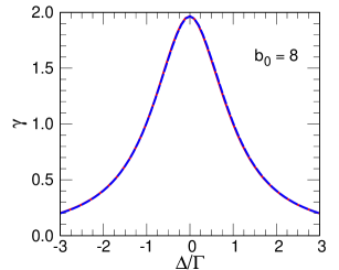
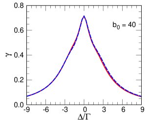
Figure 2: The total scattering rate per atom, Eq. (4), versus detuning for $\xi=1$ and for different cooperativity parameters, $b_{0}$, calculated using Eq. (2). Each plot shows the results for two different numbers of atoms: solid (red) line $N=2^{11}$ and long dashed (blue) line $N=2^{17}$. For both plots, the different calculations are nearly the same, so that the different lines are nearly indistinguishable. Plots for $b_{0}=16$, 24 and 32 and for $N>2^{11}$ showed similar level of agreement.

The maximum $\chi_{e}$ is when $\Delta^{\prime}=0$ and $\vec{r}=0$ which leads to $\chi_{e,max}=ib_{0}^{3/2}/\sqrt{6\pi N}$. This can be used to estimate how well the low density limit holds everywhere in the gas. However, this estimate can be misleading because the light does not reach the center of the cloud when $b_{0}$ is large and diffraction can be ignored. For light going on axis, the intensity is decreased by the factor of $\exp(-\xi b_{0}/2)$ when it reaches the center of the cloud for the spatially large clouds. However, atom clouds with smaller $N$ are also spatially small and diffraction becomes increasingly important, see the $b_{0}=32$ case of Fig. 1. We performed calculations for $b_{0}=8$, 16, 24, 32, and 40 although only results for 8 and 40 are given below. The $b_{0}\geq 24$ cases have negligible intensity at the center of the cloud if diffraction effects can be ignored. However, for some of our parameters, diffraction is important and light has non-negligible intensity at the cloud center for some of the large $b_{0}$ cases.

III Results

We initially present results for the dilute gas limit in order to illustrate the effects of absorption and focusing by the cloud; these calculations require larger $N$ because $\chi_{e,max}$ is inversely proportional to $\sqrt{N}$ for a fixed $b_{0}$ and $\xi$, which necessitates our iterative numerical method (see appendix, Sec. V.1). We find that, in this dilute regime, the continuum model gives excellent agreement with the point dipole model. We then show that, for dense clouds, calculations based on classical electrodynamics treatments break down. This indicates the importance of correlations between neighboring atoms induced by dipole-dipole interactions.

III.1 $\xi=1$, dilute gas limit

In this and the next section, all of the calculations of the paraxial approximation of the continuum use the low density limit of the electric susceptibility, Eq. (8). This choice is explained in Sec. III.3.

The first results are for the total scattering per atom for different number of atoms for $b_{0}=8$ and 40 and $\xi=1$. In Ref. Sutherland and Robicheaux (2016a), it was shown that the width of the resonance was $\Gamma^{\prime}=(1+b_{0}\xi/8)\Gamma$ so these calculations should give resonances from $2\times$ to $6\times$ that of the single atom resonance when $\xi=1$ and from $3\times$ to $11\times$ larger when $\xi=2$. Calculations were also done for $b_{0}=16$, 24 and 32 but are not reported because their properties can be inferred from the calculations described below. Results are reported for $2^{11}=2048$ and $2^{17}=131,072$ atoms. The calculations were averaged over many runs until a total of $2^{19}$ atoms were included in the calculation.

To give some rough sizes, the peak density times $\lambda^{3}$ gives the peak number inside a cubic wavelength. This is $(b_{0}2\pi/3)^{3/2}/\sqrt{N}$. For $b_{0}=40$ and $N=2^{17}$, there are $\sim 2$ atoms per cubic wavelength at the center of the cloud while $N=2^{11}$ gives 17 atoms per cubic wavelength. If the more relevant quantity is the density times $1/k^{3}$, then the max number is $(b_{0}/[6\pi])^{3/2}/\sqrt{N}$. By this quantity, all calculations in Fig. 2 have much less than 1 atom per $1/k^{3}$ ($\simeq 0.07$ atoms for $b_{0}=40$ and $N=2^{11}$).

Figure 2 shows plots of the total scattering rate per atom versus the detuning for 2 different cooperativity parameters: $b_{0}=8$ and 40. In each plot, there are two calculations for different values of $N$. The $N$ values are chosen to be $N=2^{11}$ and $2^{17}$. Despite the drastically different parameters for each of the clouds, the overall lineshape depends only on the value of OD. Although $N$ varies by a factor of 64, the total scattering rate per atom is essentially the same. This is because for these parameters, the eikonal approximation, Eq. (12), gives very good agreement with the calculations from randomly placed atoms. There are two interesting trends to note. The first is that the resonance line width is increasing with $b_{0}$. This effect was described in Refs. Sutherland and Robicheaux (2016a); Rehler and Eberly (1971); Scully (2007); Bromley et al. (2016). The second is that the line shape is changing with increasing $b_{0}$. For $b_{0}=8$, the line is approximated by a Lorentzian. However, for $b_{0}=40$, the central part of the line is narrower than for a Lorentzian. Also, the region near $\Delta=0$ appears to have a dependence like $|\Delta|$, instead of $\Delta^{2}$, for $b_{0}=40$. Calculations were performed for $b_{0}=16$, 24, and 32 with similar levels of agreement.

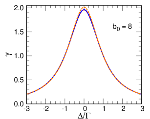
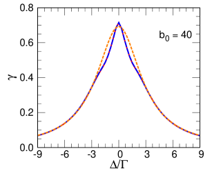
Figure 3: The total scattering rate per atom, Eq. (4), versus detuning for $\xi=1$ and for different cooperativity parameters, $b_{0}$. Each plot shows the results for the full calculation, Eq. (2), with $N=2^{17}$ solid (red) line, the model calculation, Eq. (13), long dash (blue) line, and for a Lorentzian proportional to $1/(1+(2\Delta/\Gamma^{\prime})^{2})$, dashed (orange) line. For all plots, the model and the full calculations are in such good agreement that the different lines are indistinguishable. Plots for $b_{0}=16$, 24, and 32 showed similar level of agreement.

Figure 3 shows a comparison of 3 different calculations of the total photon scattering rate, $\gamma$, versus detuning for 2 different coherence parameters: $b_{0}=8$ and 40. The solid (red) line is using the full calculation Eq. (2), with $N=2^{17}$ atoms in each run and was averaged until $2^{19}$ atoms were included. The long dash (blue) line is from the paraxial approximation in Eq. (13) substituted into Eq. (14). The resulting $\vec{P}(\vec{k})$ was then used in Eq. (6). There were no adjustable parameters. The model calculation accurately reproduces the full calculation. The dashed (orange) line is a Lorentzian using the width, $\Gamma^{\prime}=(1+b_{0}\xi/8)\Gamma$, with the height of the Lorentzian fit to give agreement in the wings. Similar results were found for $b_{0}=16$, 24, and 32.

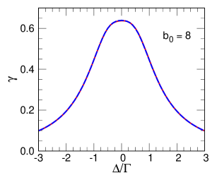
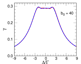
Figure 4: The forward scattering rate (see text for description) versus detuning for different cooperativity parameters, $b_{0}$. Each plot shows the results for the full calculation with $N=2^{17}$ solid (red) line and the model calculation long dash (blue) line. For all plots, the different calculations are in such good agreement that the different lines are indistinguishable. For the larger value of $b_{0}$ shown here, the scattered lineshape plateaus near-resonance, due to the fact that light does not penetrate the cloud in this regime.

Figure 3 raises an interesting point. References Scully (2007); Sutherland and Robicheaux (2016a); Bromley et al. (2016) derived the broader line width Lorentzian (dashed orange line) by solving for the superradiant time dependence uniformly excited across the Gaussian distribution of atoms (timed-Dicke state). However, neither the paraxial nor eikonal approximation of a continuum dielectric use this concept. The width in Eq. (13) is the single atom width $\Gamma$. The larger width emerging from Eq. (14) is solely due to the interplay of the non-uniform light intensity across the atom cloud as well as the phase change in Eq. (10). Figure 3 also shows that for larger values of $b_{0}$ —when the polarization ceases to significantly penetrate the full cloud —point dipole and continuous dielectric models show a narrowing of the lineshape near resonance; the timed-Dicke state models do not show this since the uniformly polarized state ansatz becomes insufficient.

The calculations allow us to untangle the coherent scattering of photons in the forward direction and the random scattering into large angles. To obtain the forward scattering rate, we integrated Eq. (4) over $\phi$ from 0 to $2\pi$ and integrated $\theta$ from 0 to $\cos(\theta_{\rm max})=1-13.8/(k^{2}r_{f}^{2})$. The $\theta_{\rm max}$ was chosen so that forward scattering has decreased by at least two orders of magnitude from its maximum value. The result is shown in Fig. 4. There is a plateau in the forward scattering rate for a range of detuning around $\Delta=0$. The atomic calculations of the forward scattering rate are, again, well reproduced by the paraxial approximation of the continuum distribution for all of the optical depths that were calculated. The eikonal approximation also agreed well with the atom calculation for the forward scattered photons except for at large $b_{0}$ and small $N$.

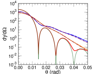
Figure 5: The angular scattering rate per atom, Eq. (4) for $b_{0}=40$ and $N=2^{17}$. There are calculations for 3 detunings: 0, 3/2, and $3\Gamma$. The solid (red) and dotted (green) lines are the atom and paraxial calculation for $\Delta=0$. The long dash (blue) and dash-dot (purple) lines are the atom and paraxial calculation for $\Delta=3\Gamma/2$. The dashed (orange) and dash-dot-dot (brown) lines are the atom and paraxial calculation for $\Delta=3\Gamma$.

Figure 5 shows the full atom calculations as well as the paraxial approximation for the angular scattering rate per atom, Eq. (4) for $b_{0}=40$ and $N=2^{17}$. This shows that coherently scattered light can be reproduced by the continuum dielectric model. The figure shows results from three different detunings. The $\Delta=0$ case shows strong diffraction minima due to the strong scattering of light in the center of the cloud; these minima are too deep for the continuum calculation because it does not include the random scattering from pointlike atoms. At large detuning, the absorption is less, so the scattered light more closely follows a Gaussian form.

III.2 $\xi=2$, dilute gas limit

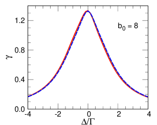
resizebox80mm!

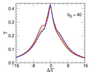
Figure 6: The total scattering rate per atom, Eq. (4), versus detuning; same as Fig. 2 except for $\xi=2$. Each plot shows the results for four different numbers of atoms: solid (red) line $N=2^{11}$, dashed (orange) line is for $N=2^{13}$, the dotted (green) line is for $N=2^{15}$, and long dashed (blue) line $N=2^{17}$.

When the Gaussian cloud is elongated in the laser propagation direction, there is more absorption and focusing of the laser beam. For $\xi=2$, the total scattering versus detuning for $N=2^{11}$, $2^{13}$, $2^{15}$, and $2^{17}$ are shown in Fig. 6. Unlike Fig. 2, the calculations with different numbers of atoms give different results for $b_{0}\geq 24$ indicating the breakdown of the eikonal approximation. In all of the calculations, the scattering rates converge to a symmetric form as $N\to\infty$, but, for smaller $N$, the scattering rate is larger for $\Delta<0$. In fact, there is a significant hump for $b_{0}=40$ at $\Delta<0$ for the $N=2^{11}$ calculation, solid (red) line. These new parametrical dependencies arise due to focusing of the light at $\Delta<0$, which correlates with a breakdown of the eikonal approximation. The focusing bends the light skirting the edge of the cloud so that it interacts more strongly with atoms to the back of the cloud than would happen without focusing: since more light goes through the cloud, there is more scattering. The focusing is also the cause of the more extreme case of the effect seen in Ref. Sutherland and Robicheaux (2016a) where atoms at the back of the cloud with $\xi\gg 1$ were more strongly excited than atoms at the front of the cloud. The effect is larger at smaller $N$ because the cloud is smaller and denser which leads to more focusing. Even more than $\xi=1$, the large $b_{0}$ scattering rate has a dependence more similar to $|\Delta|$ than to $\Delta^{2}$.

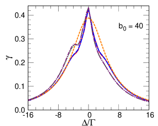
Figure 7: The total scattering rate per atom, Eq. (4), versus detuning; same as Fig. 3 but for $\xi=2$. Each plot shows the results for the full calculation, Eq. (2), ($N=2^{17}$ solid (red) line and $N=2^{11}$ dotted (green) line), for the model calculation, Eq. (13), ($N=2^{17}$ long dash (blue) line and $N=2^{11}$ dash-dot (purple) line), and for a Lorentzian proportional to $1/(1+(2\Delta/\Gamma^{\prime})^{2})$, dashed (orange) line. Note there are 5 curves plotted.

These distributions are well reproduced by the continuum dielectric model that uses the paraxial approximation. Figure 7 shows the comparison between the atomic and the continuum model calculations of the total scattering rate for $N=2^{11}$ and $2^{17}$; the continuum model calculations are nearly indistinguishable from the atomic calculations. Note that the hump at negative $\Delta$ for $N=2^{11}$ is well reproduced.

The forward scattering rate for $\xi=2$, $b_{0}=40$, and $N=2^{17}$ and $2^{11}$ are shown in Fig. 8. This has a similar form to the spherical cloud although the plateau starts at smaller $b_{0}$ (not shown). The results from the paraxial approximation to the continuum model are also shown. The $N=2^{17}$ results are in excellent agreement but there is a noticeable difference for $N=2^{11}$ and small $|\Delta|$. The difference arises when the light diffracts back into the atom cloud. We found that including the next order term did not improve the paraxial approximation which suggests that this difference is due to a breakdown of the continuum dielectric model for light propagation at higher density. The possibility that this difference arises because we use the low density form of the susceptibility, instead of Eq. (9), is addressed in the next section.

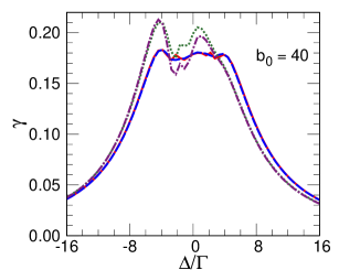
Figure 8: The forward scattering rate (see text for description) versus detuning; same as Fig. 4 but for $\xi=2$. Each plot shows the results for the full calculation ($N=2^{17}$ solid (red) line and $N=2^{11}$ dotted (green) line) and the continuum model calculation ($N=2^{17}$ long dash (blue) line and $N=2^{11}$ dash-dot (purple) line). The distributions for other $b_{0}$ have better agreement.

III.3 Denser gases

Reference Javanainen et al. (2014) showed that the Clausius-Mossotti (or Lorentz-Lorenz) form of the susceptibility, Eq. (9), does not describe the model of light scattering from stationary atoms, Eq. (2). In all of the calculations above, the paraxial approximation of the continuum model used the low density form for the susceptibility, Eq. (8). This did not make much difference in the calculations because the maximum of $\chi_{e}^{(ld)}$ was not very large. Nevertheless, we also found that the calculations using $\chi_{e}^{(ld)}$ were more accurate than using $\chi_{e}$ from Eq. (9) for smaller $N$.

Figure 9: The total scattering rate per atom, Eq. (4), versus detuning for $\xi=1$; same as Fig. 3 but for $N=2^{9}$ and $2^{7}$. Each plot shows the results for the full calculation, Eq. (2), solid (red) line, the continuum model calculation, Eq. (13), using $\chi^{(ld)}_{e}$ long dash (blue) line, and the continuum model using the Claussius-Mossotti (or Lorentz-Lorenz) electric susceptibility, Eq. (9), dashed (orange) line.

Figure 9 shows a comparison between the atom calculation (solid (red) line) and the paraxial equation using the low density electric susceptibility (long dashed (blue) line), Eq. (8), and the the Clausius-Mossotti susceptibility (dashed (orange) line), Eq. (9). The continuum calculation using the low density electric susceptibility seems to overestimate the effect from focusing for $\Delta\sim-3\Gamma$ whereas the Clausius-Mossotti susceptibility is not accurate throughout the range $|\Delta|<3\Gamma$. We found that the second order correction to the paraxial approximation did not explain the difference for $N=2^{9}$; although the correction to the paraxial approximation was not negligible for the $n=2^{7}$ calculation, it could not explain the difference with the atom calculation. Overall, the low density form of the susceptibility gives a more accurate representation of the total scattering versus detuning. The Clausius-Mossotti susceptibility gives a blue shift to the line whereas the low density form gives a slight red shift due to focusing for $\Delta<0$. The size of the effect is smaller than Ref. Javanainen et al. (2014) because they used a much higher density and they used a uniform density whereas a Gaussian density was used in this paper. The calculations in Ref. Javanainen et al. (2014) were for $\rho/k^{3}=2$ whereas Fig. 9 has $\rho_{max}/k^{3}=0.27$ for $N=2^{7}$ and 0.14 for $N=2^{9}$. These results show that the Clausius-Mossotti (or Lorentz-Lorenz) electric susceptibility does not reproduce the stationary atom calculation even in cases where $\rho/k^{3}<1$.

IV Conclusions

We have performed calculations of light scattering from a weakly driven Gaussian cloud of stationary atoms. We showed nontrivial effects on the scattering when moving from small to large optical depths. We also demonstrated a method that can solve for light scattering from many more atoms than is typical in current calculations. Thus, simulations can approach the number of atoms in experiments; results for up to $N=2^{17}$ were presented.

We showed that the photon scattering rate versus detuning is quite different from a Lorentzian at larger optical depths. This is because when poralization begins to build in the front of the cloud, the on-resonant forward scattered light does not propagate through and plateaus. For larger numbers of atoms, the total and forward scattering rates were quantitatively reproduced by a continuum model that used the low density expression for the electric susceptibility. Even though it only contains linear absorption, the continuum dielectric calculation gave better agreement with the full point dipole calculations than models that use the single photon superradiance framework. The full point dipole results for smaller atom number differ somewhat from the continuum model. Interestingly, worse results were obtained when using the Clausius-Mossotti (or Lorentz-Lorenz) form for the electric susceptibility, in agreement with the findings in Ref. Javanainen et al. (2014).

We thank J. Ruostekoski for interesting discussions about this concept and for suggesting the paraxial approximation as a method for solving the continuum model. FR was supported by the National Science Foundation under Grant No. 1804026-PHY. Part of this work was performed under the auspices of the U.S. Department of Energy by Lawrence Livermore Laboratory under Contract DE-AC52-07NA27344. LLNL-JRNL-786838-DRAFT

V Appendix

Below are more detailed description of numerical methods used in the calculations above.

V.1 Iterative method

The steady state solution of Eq. (2) involves the solution of a linear equation. For most of the calculations in this paper, we restricted the oscillators to only be in the $x$-direction which means only the terms with $j=x$ are included. The discussion in this section will focus on this case for simplicity but it should be clear how to generalize to include all polarizations. For $N$ atoms, this leads to an $N\times N$ matrix equation of the form:

$$\sum_{b}A_{b^{\prime}b}a_{b}=s_{b^{\prime}}$$ (15)

For small number of atoms (less than $\sim 1000$), we used Lapack subroutines to directly solve for $a_{b}$. For larger number of atoms, we used an iterative method based on successive over-relaxation.

The method proceeded in five stages. First, we ordered the atoms in the direction of laser propagation; for the $\vec{k}=k\hat{e}_{z}$ used above, the atoms are ordered from smallest $z$ to largest $z$; the $a_{b}$ are updated in this order so that the atom with most negative $z$ is updated first and the atom with most positive $z$ is updated last. Next, for each atom $\beta$, we found the nearest $M-1$ atoms $b^{\prime}$; these atoms will have the largest $g$ (hence, the largest $A_{b^{\prime}\beta}$). The third step constructs an $M\times M$ linear problem using the $a_{b}$ from the previous iteration. The smaller linear system is defined by

$$\tilde{A}_{b^{\prime}b} = A_{b^{\prime}b}\;{\rm for}\quad b^{\prime},b\in M$$

$$\tilde{s}_{b^{\prime}} = s_{b^{\prime}}-\sum_{b\notin M}A_{b^{\prime}b}a_{b}\quad{\rm for}\;b^{\prime}\in M$$ (16)

We next solve the much smaller linear equation

$$\sum_{b}\tilde{A}_{b^{\prime}b}\tilde{a}_{b}=\tilde{s}_{b^{\prime}}$$ (17)

using standard Lapack subroutines and update only the atom $\beta$: $a_{\beta}=(a_{\beta}+\tilde{a}_{\beta})/2$.

We order the atoms from small to large $z$ because atoms with smaller $z$ affect those at larger $z$ more strongly than vice versa. By taking them in order, the convergence speed was improved. More importantly, by directly solving Eq. (17), we are able to account for the large coupling between close pairs (or triples or quadruples etc.) of atoms.

We were able to converge all of the calculations with more than $2^{10}$ atoms using this method. Typically, we used 9 iterations before convergence. Most of the calculations converged with $M-1=7$ closest atoms. The calculations with the largest $b_{0}$ and smallest $N$ sometimes did not converge for $M=8$ but did converge for $M=16$. The calculation speed improves with smaller $M$ so we first did all calculations with $M=8$ and only repeated the failed ones with $M=16$. The failed calculations were easy to determine because they had discontinuous jumps in scattering rate versus detuning.

This algorithm was much faster than directly solving Eq. (15). This also solved the problem of memory ($A_{b^{\prime}b}$ has $N^{2}$ complex numbers); when $N$ was too large for the memory of our computer, we could compute the $A_{b^{\prime}b}$ on the fly instead of storing them in an array. Although not reported here, we did calculations with $N=2^{18}$ atoms and one test calculation with $N=2^{19}$. The calculation with $2^{19}$ atoms would require an $A$ with $\sim 1/4$ trillion elements (i.e. over a terabyte of RAM) if done by direct solution. Such large $N$ can be reached because the density decreases with $N$ which allows a smaller value of $M$ to be used. The algorithm can be parallelized; most of the calculations were done on a 4 processor workstation, but the largest calculations were done on a 20 processor workstation.

V.2 Paraxial approximation

To derive the paraxial approximation as used in this paper, start from the expression for the exact Maxwell equation, Eq. (7), and substitute the form

$$\vec{E}=E_{0}e^{ikz}\vec{\psi}\equiv E_{0}e^{ikz}(\vec{\psi}_{T}+\hat{z}\psi_{z})$$ (18)

where $\vec{a}_{T}\equiv a_{x}\hat{x}+a_{y}\hat{y}$ for any vector $\vec{a}_{T}$. This gives

$$i \frac{\partial\vec{\psi}_{T}}{\partial z}+\frac{1}{2k}\nabla_{T}^{2}\vec{\psi}_{T}+\frac{k}{2}\underline{\chi}_{e}\vec{\psi}_{T}$$ (19)

$$= -\frac{1}{2k}\frac{\partial^{2}\vec{\psi}_{T}}{\partial z^{2}}+\frac{1}{2k}\vec{\nabla}_{T}\left(\vec{\nabla}_{T}\cdot\vec{\psi}_{T}+ik\psi_{z}+\frac{\partial\psi_{z}}{\partial z}\right)$$

and

$$\psi_{z}=\frac{i}{k}\vec{\nabla}_{T}\cdot\vec{\psi}_{T}-\frac{1}{k^{2}}\nabla_{T}^{2}\psi_{z}+\frac{1}{k^{2}}\frac{\partial}{\partial z}\vec{\nabla}_{T}\cdot\vec{\psi}_{T}$$ (20)

where $\underline{\chi}_{e}\vec{\psi}_{T}\equiv\chi_{e}\psi_{x}\hat{x}$. These equations are exact but are still difficult to solve. To simplify the equations below we define the operator ${\cal B}$ as

$${\cal B}\vec{\psi}_{T}\equiv i\frac{\partial\vec{\psi}_{T}}{\partial z}+\frac{1}{2k}\nabla_{T}^{2}\vec{\psi}_{T}+\frac{k}{2}\underline{\chi}_{e}\vec{\psi}_{T}$$ (21)

We modify Eq. (19) by substituting Eq. (20) for $\psi_{z}$ to give

$$\frac{1}{k}{\cal B}\vec{\psi}_{T} = -\frac{1}{2k^{2}}\frac{\partial^{2}\vec{\psi}_{T}}{\partial z^{2}}$$

$$+ \frac{1}{2k^{2}}\vec{\nabla}_{T}\left(-\frac{i}{k}\nabla_{T}^{2}\psi_{z}+\frac{i}{k}\frac{\partial}{\partial z}\vec{\nabla}_{T}\cdot\vec{\psi}_{T}+\frac{\partial\psi_{z}}{\partial z}\right)$$

To obtain the paraxial approximation, one scales $x,y$ by a width ${\rm w}$ and $z$ by a length $L\equiv{\rm w}/f$ (i.e. $x={\rm w}\bar{x}$, $y={\rm w}\bar{y}$, and $z=L\bar{z}$ with the barred coordinates being dimensionless). The ratio ${\rm w}/L=f$ is set equal to $f\equiv 1/(k{\rm w})$. For the paraxial approximation, $f$ should be small which means the distance scale of variations in $x,y$ should be large compared to $1/k$ and the distance scale of variations in $z$ should be large compared to that in $x,y$. Substituting this scaling into the differential equations suggests that the three terms on the right hand side of Eq. (20) are of order $f^{1}$, $f^{2}$, and $f^{3}$ respectively. The terms on the left hand side of Eq. (V.2) are of order $f^{0}$ or $f^{2}$ and on the right hand side are of order $f^{3}$ if they involve $\psi_{z}$ and $f^{4}$ if they involve $\vec{\psi}_{T}$.

The functions are written as a series

$$\vec{\psi}_{T} = \vec{\psi}_{T}^{(0)}+\vec{\psi}_{T}^{(2)}+\vec{\psi}_{T}^{(4)}+...$$

$$\psi_{z} = \psi_{z}^{(1)}+\psi_{z}^{(3)}+\psi_{z}^{(5)}+...$$ (23)

To obtain the equations for the different terms, one groups the same orders together. For example, since the first term on the right hand side of Eq. (20) is of order $f^{1}$, a term like $(i/k)\vec{\nabla}_{T}\cdot\vec{\psi}_{T}^{(4)}$ is of order 5 since the $\vec{\psi}_{T}$ is order 4 and the operation is of order 1. Equation (20) is transformed to

$$\psi_{z}^{(n)}=\frac{i}{k}\vec{\nabla}_{T}\cdot\vec{\psi}_{T}^{(n-1)}-\frac{1}{k^{2}}\nabla_{T}^{2}\psi_{z}^{(n-2)}+\frac{1}{k^{2}}\frac{\partial}{\partial z}\vec{\nabla}_{T}\cdot\vec{\psi}_{T}^{(n-3)}$$ (24)

when grouping terms of order $n$. Defining the order of the $(1/k){\cal B}$ operator is somewhat problematic due to the $\chi_{e}$ term. We take it to be an order 2 operator, consistent with the two differential terms. Equation (V.2) is transformed to

$$\frac{1}{k}{\cal B}\vec{\psi}_{T}^{(n)}= - \frac{1}{2k^{2}}\frac{\partial^{2}\vec{\psi}_{T}^{(n-2)}}{\partial z^{2}}+\frac{1}{2k^{2}}\vec{\nabla}_{T}(-\frac{i}{k}\nabla_{T}^{2}\psi_{z}^{(n-1)}$$ (25)

$$+ \frac{i}{k}\frac{\partial}{\partial z}\vec{\nabla}_{T}\cdot\vec{\psi}_{T}^{(n-2)}+\frac{\partial\psi_{z}^{(n-1)}}{\partial z})$$

when grouping terms of order $n+2$. If $n=0$, 1, or 2, the functions on the right hand side can have negative superscript. The rule for evaluating these are: any function with a negative superscript is zero everywhere.

The case discussed in the paper has the atoms only being polarizable in the $x$-direction. This means all of the quantities of interest can be calculated from the $\psi_{x}$. Thus, through order 2, the equations to be solved are

$${\cal B}\hat{x}\psi_{x}^{(0)} = 0\qquad\psi_{y}^{(0)}=0$$

$$\psi_{z}^{(1)} = \frac{i}{k}\frac{\partial\psi_{x}^{(0)}}{\partial x}$$

$${\cal B}\hat{x}\psi_{x}^{(2)} = -\frac{1}{2k}\left(\frac{\partial^{2}\psi_{x}^{(0)}}{\partial z^{2}}+\frac{\partial^{2}[\chi_{e}\psi_{x}^{(0)}]}{\partial x^{2}}\right)\hat{x}$$ (26)

with the $\psi_{x}^{(2)}$ set to 0 as $z\to-\infty$. Note the $\psi_{y}^{(2)}$ is nonzero, but it is not used in our calculations.

References

- Dicke (1954) R. H. Dicke, “Coherence in spontaneous radiation processes,” Phys. Rev. 93, 99 (1954).
- Rehler and Eberly (1971) N. E. Rehler and J. H. Eberly, “Superradiance,” Phys. Rev. A 3, 1735 (1971).
- Gross and Haroche (1982) M. Gross and S. Haroche, “Superradiance: An essay on the theory of collective spontaneous emission,” Phys. Rep. 93, 301 (1982).
- Sutherland and Robicheaux (2017a) R. T. Sutherland and F. Robicheaux, “Superradiance in inverted multilevel atomic clouds,” Phys. Rev. A 95, 033839 (2017a).
- Ruostekoski and Javanainen (1997) J. Ruostekoski and J. Javanainen, “Quantum field theory of cooperative atom response: low light intensity,” Phys. Rev. A 55, 513 (1997).
- Scully et al. (2006) M. O. Scully, E. S. Fry, C. H. R. Ooi, and K. Wódkiewicz, “Directed spontaneous emission from an extended ensemble of atoms: Timing is everything,” Phys. Rev. Lett. 96, 010501 (2006).
- Scully (2007) M.O. Scully, “Correlated spontaneous emission on the Volga,” Laser Phys. 17, 635 (2007).
- Sutherland and Robicheaux (2016a) R. T. Sutherland and F. Robicheaux, “Coherent forward broadening in cold atom clouds,” Phys. Rev. A 93, 023407 (2016a).
- Sutherland and Robicheaux (2016b) R. T. Sutherland and F. Robicheaux, “Collective dipole-dipole interactions in an atomic array,” Phys. Rev. A 94, 013847 (2016b).
- Bromley et al. (2016) S. L. Bromley, B. Zhu, M. Bishof, X. Zhang, T. Bothwell, J. Schachenmayer, T. L. Nicholson, R. Kaiser, S. F. Yelin, M. D. Lukin, et al., “Collective atomic scattering and motional effects in a dense coherent medium,” Nat. Commun. 7, 11039 (2016).
- Bettles et al. (2016) R. J. Bettles, S. A. Gardiner, and C. S. Adams, “Enhanced optical cross section via collective coupling of atomic dipoles in a 2d array,” Phys. Rev. Lett. 116, 103602 (2016).
- Svidzinsky and Chang (2008) A. Svidzinsky and J.-T. Chang, “Cooperative spontaneous emission as a many-body eigenvalue problem,” Phys. Rev. A 77, 043833 (2008).
- Jenkins and Ruostekoski (2012a) S. D. Jenkins and J. Ruostekoski, “Controlled manipulation of light by cooperative response of atoms in an optical lattice,” Phys. Rev. A 86, 031602 (2012a).
- Sutherland and Robicheaux (2017b) R. T. Sutherland and F. Robicheaux, “Degenerate Zeeman ground states in the single-excitation regime,” Phys. Rev. A 96, 053840 (2017b).
- Zhu et al. (2016) B. Zhu, J. Cooper, J. Ye, and A. M. Rey, “Light scattering from dense cold atomic media,” Phys. Rev. A 94, 023612 (2016).
- Meir et al. (2014) Z. Meir, O. Schwartz, E. Shahmoon, D. Oron, and R. Ozeri, “Cooperative Lamb shift in a mesoscopic atomic array,” Phys. Rev. Lett. 113, 193002 (2014).
- Anderson (1958) P. W. Anderson, “Absence of diffusion in certain random lattices,” Phys. Rev. 109, 1492 (1958).
- Störzer et al. (2006) M. Störzer, P. Gross, C. M. Aegerter, and G. Maret, “Observation of the critical regime near anderson localization of light,” Phys. Rev. Lett. 96, 063904 (2006).
- Skipetrov and Sokolov (2015) S.E. Skipetrov and I.M. Sokolov, “Magnetic-field-driven localization of light in a cold-atom gas,” Phys. Rev. Lett. 114, 053902 (2015).
- Jackson (1999) J. D. Jackson, Classical Electrodynamics, 3rd Edition (John Wiley & Sons, 1999).
- Mie (1908) G. Mie, “BeitrÀge zur optik trÃŒber medien, speziell kolloidaler metallösungen,” Annalen der Physik 330, 377–445 (1908).
- Friedberg et al. (1973) R. Friedberg, S. R. Hartmann, and J. T. Manassah, “Frequency shifts in emission and absorption by resonant systems of two-level atoms,” Phys. Rep. 7, 101 (1973).
- Cottier et al. (2018) F. Cottier, R. Kaiser, and R. Bachelard, “Role of disorder in super- and subradiance of cold atomic clouds,” Phys. Rev. A 98, 013622 (2018).
- Javanainen et al. (2014) J. Javanainen, J. Ruostekoski, Y. Li, and S.-M. Yoo, “Shifts of a resonance line in a dense atomic sample,” Phys. Rev. Lett. 112, 113603 (2014).
- Javanainen and Ruostekoski (2016) J. Javanainen and J. Ruostekoski, “Light propagation beyond the mean-field theory of standard optics,” Opt. Express 24, 993 (2016).
- Svidzinsky et al. (2010) A. A. Svidzinsky, J.-T. Chang, and M. O. Scully, “Cooperative spontaneous emission of atoms: Many-body eigenstates, the effect of virtual Lamb shift processes, and analogy with radiation of classical oscillators,” Phys. Rev. A 81, 053821 (2010).
- Jenkins and Ruostekoski (2012b) S. D. Jenkins and J. Ruostekoski, “Controlled manipulation of light by cooperative response of atoms in an optical lattice,” Phys. Rev. A 86, 031602 (2012b).
- Rouabah et al. (2014) M.-T. Rouabah, M. Samoylova, R. Bachelard, P. W. Courteille, R. Kaiser, and N. Piovella, “Coherence effects in scattering order expansion of light by atomic clouds,” J. Opt. Soc. Am. A 31, 1031 (2014).
- Lee et al. (2016) M. D. Lee, S. D. Jenkins, and J. Ruostekoski, “Stochastic methods for light propagation and recurrent scattering in saturated and nonsaturated atomic ensembles,” Phys. Rev. A 93, 063803 (2016).
- Loudon (2000) R. Loudon, The Quantum Theory of Light, 3rd Edition (Oxford University Press, New York, 2000).
- Lax et al. (1975) M. Lax, W. H. Louisell, and W. B. McKnight, “From Maxwell to paraxial wave optics,” Phys. Rev. A 11, 1365 (1975).