On Rank Estimators in Increasing Dimensions

Abstract

The family of rank estimators, including Han’s maximum rank correlation (Han,, 1987) as a notable example, has been widely exploited in studying regression problems. For these estimators, although the linear index is introduced for alleviating the impact of dimensionality, the effect of large dimension on inference is rarely studied. This paper fills this gap via studying the statistical properties of a larger family of M-estimators, whose objective functions are formulated as U-processes and may be discontinuous in increasing dimension set-up where the number of parameters, $p_{n}$, in the model is allowed to increase with the sample size, $n$. First, we find that often in estimation, as $p_{n}/n\rightarrow 0$, $(p_{n}/n)^{1/2}$ rate of convergence is obtainable. Second, we establish Bahadur-type bounds and study the validity of normal approximation, which we find often requires a much stronger scaling requirement than $p_{n}^{2}/n\rightarrow 0$. Third, we state conditions under which the numerical derivative estimator of asymptotic covariance matrix is consistent, and show that the step size in implementing the covariance estimator has to be adjusted with respect to $p_{n}$. All theoretical results are further backed up by simulation studies.

Keywords: Bahadur-type bounds, degenerate U-processes, maximal inequalities, uniform bounds.

JEL Codes: C55, C14.

1 Introduction

1.1 The General Set-up, Motivation, and Main Results

Let $\bm{Z}_{1},\ldots,\bm{Z}_{n}\in{\mathbb{R}}^{m_{n}}$ denote a random sample of size $n$ from the probability measure $\mathbb{P}$. Let $\mathcal{F}:=\{f(\cdot,\cdot;\bm{\theta}):\bm{\theta}\in\Theta\subset{\mathbb{R}}^{p_{n}}\}$ be a class of real-valued, possibly asymmetric and discontinuous, functions on ${\mathbb{R}}^{m_{n}}\times{\mathbb{R}}^{m_{n}}$. This paper studies the following M-estimator with an objective function of a U-process structure,

$$\widehat{\bm{\theta}}_{n}:=\mathop{\mathrm{argmax}}_{\bm{\theta}\in\Theta}\Gamma_{n}(\bm{\theta})=\mathop{\mathrm{argmax}}_{\bm{\theta}\in\Theta}\frac{1}{n(n-1)}\sum_{i\neq j=1}^{n}f(\bm{Z}_{i},\bm{Z}_{j};\bm{\theta}).$$ (1.1)

Let

$$\bm{\theta}_{0}:=\mathop{\mathrm{argmax}}_{\bm{\theta}\in\Theta}\Gamma(\bm{\theta})=\mathop{\mathrm{argmax}}_{\bm{\theta}\in\Theta}\mathbb{E}\Gamma_{n}(\bm{\theta}).$$

This paper aims to establish asymptotic properties of $\widehat{\bm{\theta}}_{n}$ as an estimator of $\bm{\theta}_{0}$ in situations with large or increasing dimensions $m_{n}\rightarrow\infty$ and $p_{n}\rightarrow\infty$ (with respect to the sample size $n$), to which existing results do not apply.

Members of (1.1) include the following notable examples proposed and studied in the current literature in fixed dimension, i.e., $m_{n}\equiv m$ and $p_{n}\equiv p$ for all $n$: (1) Han’s maximum rank correlation (MRC) estimator for the generalized regression model (Han,, 1987); (2) Cavanagh and Sherman’s rank estimator for the same model as Han’s (Cavanagh and Sherman,, 1998); (3) Khan and Tamer’s rank estimator for the semiparametric censored duration model (Khan and Tamer,, 2007); and (4) Abrevaya and Shin’s rank estimator for the generalized partially linear index model (Abrevaya and Shin,, 2011). One common feature of these models is the presence of a linear index of the form $\bm{x}^{\top}\bm{\theta}$, where $\bm{x}$ represents covariates of dimension $p$ which is typically large in many economic applications. The linear index structure is introduced to alleviate the “curse of dimensionality” associated with fully nonparametric models. Although motivated by possibly large dimension $p$, properties of $\widehat{\bm{\theta}}_{n}$ in these examples have only been established for fixed $p$ when $n$ approaches infinity (i.e., $p$ does not change with $n$). Instead, this paper models the large $p$ case by allowing $p$ to go to infinity as $n\rightarrow\infty$, denoted as $p_{n}$, facilitating an explicit characterization of the effect of dimensionality on inference in these models.

More broadly, for the general set-up (1.1), we allow both $m_{n}$ and $p_{n}$ to go to infinity as $n\rightarrow\infty$ and establish the following properties of $\widehat{\bm{\theta}}_{n}$: (i) consistency; (ii) rate of convergence; (iii) normal approximation; and (iv) accuracy of normal approximation. The last property is also referred to as the “Bahadur-Kiefer representation” or simply the “Bahadur-type bound” (Bahadur,, 1966; Kiefer,, 1967; He and Shao,, 1996), and is the major focus of this paper. Specifically, in Theorems 2.2, 2.3, and 2.4, under different scaling requirements for $n$, $p_{n}$, and $\nu_{n}$, where $\nu_{n}$ characterizes the function complexity of $\mathcal{F}$, we prove consistency, efficient rate of convergence, and derive Bahadur-type bounds for the general M-estimator $\widehat{\bm{\theta}}_{n}$ of the form (1.1). To facilitate inference, we construct consistent estimators of the asymptotic covariance matrix of $\widehat{\bm{\theta}}_{n}$ similar to the numerical derivative estimators in Pakes and Pollard, (1989), Sherman, (1993), and Khan and Tamer, (2007). The increasing dimension set-up in this paper reveals that for consistent variance-covariance matrix estimation, the step size in computing the numerical derivative should depend not only on the sample size $n$ but also the dimensions $m_{n}$ and $p_{n}$.

To provide further insight on the role of the dimension $p_{n}$, we apply our general results, Bahadur-type bounds especially, to the aforementioned rank estimators (1)-(4). Note that for these estimators $\nu_{n}=m_{n}=p_{n}$. Corollaries 3.1–3.4 provide sufficient conditions to guarantee consistency, efficient rate of convergence, and asymptotic normality (ASN) of the rank correlation estimators in increasing dimension. They demonstrate that, compared to competing alternatives such as simple linear regression, in terms of estimation, rank estimators are very appealing, maintaining the minimax optimal $(p_{n}/n)^{1/2}$ rates (Yu,, 1997), while enjoying an additional robustness property to outliers and modeling assumptions. With regard to normal approximation, on the other hand, a much stronger scaling requirement might be needed, and a lower accuracy in normal approximation is anticipated. This observation also echoes a common belief in robust statistics that stronger scaling requirement than $p_{n}^{2}/n\rightarrow 0$ is needed for normal approximation validity (Jurečková et al.,, 2012).

All the theoretical results are further backed up by simulation studies. In particular, using Han’s MRC estimator introduced below, we have demonstrated that for a given sample size, the accuracy of the normal approximation deteriorates quickly as the number of parameters $p_{n}$ increases, indicating that our theoretical bound is difficult to improve further. Also, our simulation results suggest that for variance estimation, the step size needs to be adjusted with respect to $p_{n}$. Practically, our results indicate that although the linear index was introduced to alleviate the curse of dimensionality, one must be cautious in conducting inference using rank estimators when there are many covariates.

1.2 The Generalized Regression Model and Han’s MRC

Han’s MRC in Example (1) is the first rank correlation estimator proposed to estimate the parameter $\bm{\beta}_{0}$ in the generalized regression model:

$$Y=D\circ F(\bm{X}^{\top}\bm{\beta}_{0},\epsilon),$$ (1.2)

where $\bm{\beta}_{0}\in\mathbb{R}^{p_{n}+1}$, $F(\cdot,\cdot)$ is a strictly increasing function of each of its arguments, and $D(\cdot)$ is a non-degenerate monotone increasing function of its argument. Important members of the generalized regression model in (1.2) include many widely known and extensively used econometrics models in diverse areas in empirical microeconomics such as the binary choice models, the ordered discrete response models, transformation models with unknown transformation functions, the censored regression models, and proportional and additive hazard models under the independence assumption and monotonicity constraints. 

Han, (1987) proposed estimating $\bm{\beta}_{0}$ in (1.2) with

$$\widehat{\bm{\beta}}_{n}^{\mathsf{H}}=\mathop{\mathrm{argmax}}_{\bm{\beta}:\beta_{1}=1}\Big{\{}\frac{1}{n(n-1)}\sum_{i\neq j}\mathds{1}(Y_{i}>Y_{j})\mathds{1}(\bm{X}_{i}^{\top}\bm{\beta}>\bm{X}_{j}^{\top}\bm{\beta})\Big{\}}.$$ (1.3)

For model identification, following Sherman, (1993), we assume the first component of $\bm{\beta}_{0}$ is equal to 1, and express $\bm{\beta}_{0}$ as $\bm{\beta}_{0}=(1,\bm{\theta}_{0}^{\top})^{\top}$. We consider estimating $\bm{\theta}_{0}$ by $\widehat{\bm{\theta}}_{n}^{\mathsf{H}}:=\widehat{\bm{\beta}}_{n,-1}^{\mathsf{H}}$, the subvector of $\widehat{\bm{\beta}}_{n}^{\mathsf{H}}$ excluding its first component. We will use the generalized regression model (1.2) and Han’s MRC $\widehat{\bm{\theta}}_{n}^{\mathsf{H}}$ to illustrate our notation, assumptions, and main results in Section 2. We defer a rigorous analysis of Han’s estimator including verification of assumptions to Section 3 which also presents results for the other three rank correlation estimators.

Empirically, consider estimating the individual demand curve for a durable good such as a refrigerator. Let $Y_{i}$ be whether the individual $i$ buys a refrigerator and $\bm{X}_{i}$ be the vector of characteristics of the individual and the refrigerator included in the model. There are many potential candidates for the components of $\bm{X}_{i}$ such as personal income, marital status, the number of children, space of the kitchen, food habits; size of the refrigerator, temperature controls, lighting, shelves, dairy compartment, chiller, door styles. Assuming a single index form with $m_{n}=p_{n}+1$, this binary choice model falls into our framework with (1.2). Our increasing dimension set-up allows more characteristics to be included in $\bm{X}_{i}$ as the sample size $n$ increases and our results show that even with the single index form, estimation and inference are possible if $p_{n}$ increases very mildly with $n$ but otherwise are very challenging.

1.3 A Brief Review of Related Works and Technical Challenge

In contrast with the fixed dimension setting, where the model is assumed unchanged as $n$ goes to infinity, the increasing dimension triangular array setting (Portnoy,, 1984; Fan et al.,, 2015; Chernozhukov et al.,, 2015, 2017) makes our analysis different from and more challenging than most existing ones (cf. Theorem 3.2.16 and Example 3.2.22 in van der Vaart and Wellner, (1996), or the main theorem in He and Shao, (1996)). Technically, this paper builds on and contributes to two distinct literatures: the literature on estimation and inference in increasing dimension where existing works exclude discontinuous loss functions and the literature on rank estimation where existing works focus exclusively on finite dimensions. As a technical contribution, we establish a maximal inequality, yielding a uniform bound for degenerate U-processes in increasing dimensions which not only allows us to extend existing results on rank estimation in finite dimension to increasing dimensions but also establish Bahadur-type bounds. Besides the crucial role played by our new maximal inequality for degenerate U-processes in this paper, it should prove to be an indispensible tool in nonparametric and semiparametric econometrics in increasing dimensions where many estimators and test statistics are closely related to U-processes.

Since Huber’s seminal paper (Huber,, 1973), there has been a long history in statistics on evaluating the impact of parameter dimension on inference. Huber himself raised questions on the scaling limits of $(n,p_{n})$ for assuring M-estimation consistency and asymptotic normality in his 1973 paper (Huber,, 1973). For addressing them, Portnoy, (1984), Portnoy, (1985), Mammen, (1989), and Mammen, (1993) studied the linear regression model using smooth M-estimators such as the ordinary least squares. Their results revealed that, in response to Huber’s question, for the simple linear regression model, asymptotic normality is usually attainable even when $p_{n}^{2}/n$ is large. In contrast, Portnoy, (1988) studied maximum likelihood estimators of generalized linear models, and proved that, for guaranteeing the validity of normal approximation, the requirement $p_{n}^{2}/n\rightarrow 0$ is in general unrelaxable. Different from the analysis in large $p_{n}^{2}/n$ setting, the techniques in Portnoy, (1988) are applicable to more general cases. For example, focusing on the general likelihood problem with a differentiable likelihood function, Spokoiny, 2012a has provided a finite-sample analysis of normal approximation accuracy. Related results have also been developed in He and Shao, (2000). As a direct consequence, a set of regularity conditions could be derived for constructing Bahadur-type bounds, guaranteeing ASN provided some scaling requirements hold.

Extending existing works allowing for increasing parameter dimension, this paper studies asymptotic properties of $\widehat{\bm{\theta}}_{n}$ in (1.1), allowing both $m_{n}$ and $p_{n}$ to go to infinity as $n\rightarrow\infty$. The potential discontinuity and U-process structure of the objective function $\Gamma_{n}(\bm{\theta})$ prevent results or the proof strategy in the current literature on increasing parameter dimension from being directly applicable. On the other hand, for (1.1), the increasing dimension set-up in this paper poses technical challenges to the proof strategy adopted for fixed $m_{n}$ and $p_{n}$ exclusively studied in the current literature. To see this, recall that the main argument used in the current literature to establish asymptotic properties for estimators of the form (1.1) for fixed $m_{n}$ and $p_{n}$ follows Sherman (Sherman,, 1993, 1994), which relies on the Hoeffding decomposition, a uniform bound for degenerate U-processes, and the classical M-estimation framework tracing back to Huber’s seminal paper, Huber, (1967). Specifically, for the statistic $\Gamma_{n}(\bm{\theta})$ in (1.1), Hoeffding, (1948) derived the following well-known expansion now known as the Hoeffding decomposition:

$$\Gamma_{n}(\bm{\theta})=\Gamma(\bm{\theta})+\mathbb{P}_{n}g(\cdot;\bm{\theta})+\mathbb{U}_{n}h(\cdot,\cdot;\bm{\theta}),$$ (1.4)

where

$$g(\bm{z};\bm{\theta}) :=\mathbb{E}f(\bm{z},\cdot;\bm{\theta})+\mathbb{E}f(\cdot,\bm{z};\bm{\theta})-2\Gamma(\bm{\theta}),$$

$$h(\bm{z}_{1},\bm{z}_{2};\bm{\theta}) :=f(\bm{z}_{1},\bm{z}_{2};\bm{\theta})-\mathbb{E}f(\bm{z}_{1},\cdot;\bm{\theta})-\mathbb{E}f(\cdot,\bm{z}_{2};\bm{\theta})+\Gamma(\bm{\theta}),$$ (1.5)

$$\mathbb{P}_{n}g(\cdot;\bm{\theta}) :=\sum_{i=1}^{n}g(\bm{Z}_{i})/n,\text{ and}$$

$$\mathbb{U}_{n}h(\cdot,\cdot;\bm{\theta}) :=\sum_{i\neq j=1}^{n}h(\bm{Z}_{i},\bm{Z}_{j};\bm{\theta})/\{n(n-1)\}.$$

Hoeffding, (1948) further showed that for fixed $m_{n}$ and $p_{n}$,

$$\Gamma_{n}(\bm{\theta})\approx\underbrace{\Gamma(\bm{\theta})+\mathbb{P}_{n}g(\cdot;\bm{\theta})}_{\widetilde{\Gamma}_{n}(\bm{\theta})},$$ (1.6)

where the remainder term $\mathbb{U}_{n}h(\cdot,\cdot;\bm{\theta})$, formulated as a degenerate U-statistic, is asymptotically negligible in large samples. As a result, $\widehat{\bm{\theta}}_{n}$ is asymptotically equivalent to $\widetilde{\bm{\theta}}_{n}$ defined below:

$$\widetilde{\bm{\theta}}_{n}:=\mathop{\mathrm{argmax}}_{\bm{\theta}\in\Theta}\widetilde{\Gamma}_{n}(\bm{\theta}).$$ (1.7)

Sherman (Sherman,, 1993, 1994) was the first to notice that, by (1.4) and the negligibility of $\mathbb{U}_{n}h(\cdot,\cdot;\bm{\theta})$, the U-statistic formulation has intrinsically helped smooth the loss function in (1.1) from $\Gamma_{n}(\bm{\theta})$ to $\widetilde{\Gamma}_{n}(\bm{\theta})$, and hence renders an asymptotically normal estimator $\widehat{\bm{\theta}}_{n}$, even though the original loss function $\Gamma_{n}(\bm{\theta})$ may not be differentiable.

For increasing dimensions $m_{n}$ and $p_{n}$, the Hoeffding decomposition of $\ \Gamma_{n}(\bm{\theta})$ takes the same form as in the case of fixed $m_{n}$ and $p_{n}$. However existing maximal inequalities or uniform bounds for degenerate U-processes for finite dimensions crucial to Sherman (Sherman,, 1993, 1994) and the classical M-estimation theory for finite dimensions are inapplicable. In response to the first challenge, this paper develops a maximal inequality, yielding a uniform bound for degenerate U-processes in increasing dimensions, which allows us to show that under regularity conditions, $\widehat{\bm{\theta}}_{n}$ is asymptotically equivalent to $\widetilde{\bm{\theta}}_{n}$. Due to the smoothness of $\widetilde{\Gamma}_{n}(\bm{\theta})$, we are able to build on and improve arguments used in the proofs of Spokoiny, 2012a on M-estimators with differentiable objective functions in increasing dimensions to establish asymptotic properties of $\widetilde{\bm{\theta}}_{n}$.

1.4 Notation

For a set $\mathcal{S}$, denote its binary Cartesian product as $\mathcal{S}\otimes\mathcal{S}$. For a probability measure $\mathbb{P}$, denote its product measure as $\mathbb{P}\otimes\mathbb{P}$. For $q\in[1,\infty]$, the $L_{q}$-norm of a vector $\bm{\beta}$ is denoted by $\|\bm{\beta}\|_{q}$. The $L_{q}$-induced matrix operator norm of a matrix $\mathbf{A}$ is denoted by $\|\mathbf{A}\|_{q}$. One example is the spectral norm $\|\mathbf{A}\|_{2}$, which represents the maximal singular value of $\mathbf{A}$. In the sequel, when no confusion is possible, we will omit the subscript in the $L_{q}$-norm of $\bm{\beta}$ or $\mathbf{A}$ when $q=2$. The minimum and maximum eigenvalues of a real symmetric matrix are denoted by $\lambda_{\min}(\cdot)$ and $\lambda_{\max}(\cdot)$ respectively. Let $\mathbf{I}_{p}$ denote the $p\times p$ identity matrix. Let $\mathbb{S}^{p-1}$ denote the unit-sphere of ${{\mathbb{R}}}^{p}$ under $\|\cdot\|$. For a twice differentiable real-valued function $\tau(\bm{\theta})$, let $\nabla_{1}\tau(\bm{\theta})$ denote the vector of partial derivatives $(\partial\tau/\partial\theta_{1},\ldots,\partial\tau/\partial\theta_{p})^{\top}$ and $\nabla_{2}\tau(\bm{\theta})$ denote the Hessian matrix of $\tau(\bm{\theta})$. Let $\mathcal{B}(\bm{\theta}_{0},r)=\{\bm{\theta}\in\Theta,\|\bm{\theta}-\bm{\theta}_{0}\|<r\}$ denote an open ball of radius $r>0$ centered at $\bm{\theta}_{0}\in\Theta$, and let $\overline{\mathcal{B}}(\bm{\theta}_{0},r)=\{\bm{\theta}\in\Theta,\|\bm{\theta}-\bm{\theta}_{0}\|\leq r\}$ denote a closed ball of center $\bm{\theta}_{0}$ and radius $r$. For two real numbers $a$ and $b$, we define $a\vee b=\max(a,b)$ and $a\wedge b=\min(a,b)$. We use $\xrightarrow{\mathbb{P}}$ to denote convergence in probability with respect to $\mathbb{P}$, and $\Rightarrow$ to denote convergence in distribution. For any two real sequences $\{a_{n}\}$ and $\{b_{n}\}$, we write $a_{n}=O(b_{n})$ if there exists an absolute positive constant $C$ such that $|a_{n}|\leq C|b_{n}|$ for any large enough $n$. We write $a_{n}\asymp b_{n}$ if both $a_{n}=O(b_{n})$ and $b_{n}=O(a_{n})$ hold. We write $a_{n}=o(b_{n})$ if for any absolute positive constant $C$, we have $|a_{n}|\leq C|b_{n}|$ for any large enough $n$. We write $a_{n}=O_{\mathbb{P}}(b_{n})$ and $a_{n}=o_{\mathbb{P}}(b_{n})$ if $a_{n}=O(b_{n})$ and $a_{n}=o(b_{n})$ hold stochastically. We let $C,C^{\prime},C^{\prime\prime},c,c^{\prime},c^{\prime\prime},\ldots$ be generic absolute positive constants, whose values will vary at different locations.

1.5 Paper Organization

The rest of this paper is organized as follows. In Section 2, we introduce general methods for handling M-estimators of the particular format. In particular, Section 2.1 gives a new U-process bound in increasing dimensions, and Section 2.2 studies M-estimators of the form (1.1), whose loss functions are possibly discontinuous. Section 3 applies the results in Section 2 to the four motivating rank estimators. Section 4 offers detailed finite-sample studies, illustrating the impact of dimension on coverage probability and tuning parameter selection in the asymptotic covariance estimation. Concluding remarks and possible extensions are put in the end of the main text. All proofs are relegated to an appendix.

2 Asymptotic Theory for the M-estimator

Recall that $\bm{Z}_{1},\bm{Z}_{2},\ldots,\bm{Z}_{n}\in{\mathbb{R}}^{m_{n}}$ is a random sample from $\mathbb{P}$, rendering an empirical measure $\mathbb{P}_{n}$. Let $\mathcal{F}=\{f(\cdot,\cdot;\bm{\theta}):\bm{\theta}\in\Theta\subset{{\mathbb{R}}}^{p_{n}}\}$ be a VC-subgraph class of real-valued functions, with $\nu_{n}$ denoting the $VC$-dimension of $\mathcal{F}$ (see Section 2.6.2 in van der Vaart and Wellner, (1996) for explicit definitions of VC-subgraph and VC-dimension of a VC-subgraph class). In addition, we assume the function class $\mathcal{F}$ to be uniformly bounded by an absolute constant. The family of bounded VC-subgraph classes includes, as subfamilies, those rank estimators proposed in Han, (1987), Cavanagh and Sherman, (1998), Khan and Tamer, (2007), and Abrevaya and Shin, (2011), and suffices for our purpose.

Without loss of generality, we assume that

$$f(\bm{z}_{1},\bm{z}_{2};\bm{\theta}_{0})=0~{}~{}\mathrm{for~{}all~{}}(\bm{z}_{1},\bm{z}_{2})\in{\mathbb{R}}^{m_{n}}\otimes{\mathbb{R}}^{m_{n}},$$ (2.1)

which can always be arranged by working with $f(\bm{z}_{1},\bm{z}_{2};\bm{\theta})-f(\bm{z}_{1},\bm{z}_{2};\bm{\theta}_{0})$ throughout.

The derivation of asymptotic properties of $\widehat{\bm{\theta}}_{n}$ can be understood in two steps. First we show the asymptotic equivalence of $\widehat{\bm{\theta}}_{n}$ and $\widetilde{\bm{\theta}}_{n}$ by proving negligibility of $\mathbb{U}_{n}h(\cdot,\cdot;\bm{\theta})$ and then establish asymptotic properties of $\widetilde{\bm{\theta}}_{n}$. Essential to the first step is an increasing dimension analogue of maximal inequalities for degenerate U-processes in finite dimensions. Because of increasing dimensions, we need to calculate an exact order of the decaying rate of $\sup_{\bm{\theta}}|\mathbb{U}_{n}h(\cdot,\cdot;\bm{\theta})|$ in a local neighborhood of $\bm{\theta}_{0}$, the proof of which requires a substantial amount of modifications to the decoupling arguments in Nolan and Pollard, (1987). For the second step, we exploit Spokoiny’s bracketing device technique (cf. Corollary 2.2 in Spokoiny, 2012b ) on M-estimators with differentiable objective functions.

2.1 A Maximal Inequality for Degenerate U-processes

For fixed dimensions, Sherman (Sherman,, 1993, 1994) proved a maximal inequality for degenerate U-processes and used it to show that, when $\mathcal{F}$ is $\mathbb{P}$-Donsker (Dudley,, 1999), uniformly over a small neighborhood $\Theta_{0}$ surrounding $\bm{\theta}_{0}$,

$$\sup_{\bm{\theta}\in\Theta_{0}}|\Gamma_{n}(\bm{\theta})-\widetilde{\Gamma}_{n}(\bm{\theta})|=\sup_{\bm{\theta}\in\Theta_{0}}|\mathbb{U}_{n}h(\cdot,\cdot;\bm{\theta})|=o_{\mathbb{P}}(1/n),$$ (2.2)

which, combined with the fact that $g(\cdot)$ is usually a smooth function by integration, is sufficient to guarantee that the stochastic differentiability condition (cf. Theorem 3.2.16 in van der Vaart and Wellner, (1996)) holds. This suffices for establishing ASN in fixed dimension. However, when we allow the dimension to increase with the sample size, (2.2) is no longer correct.

To account for the effect of increasing dimension, we establish a new maximal inequality for degenerate U-processes in increasing dimensions. Theorem 2.1 below works out an exact order of the rate of convergence of $\sup_{\bm{\theta}\in\Theta_{0}}|\mathbb{U}_{n}h(\cdot,\cdot;\bm{\theta})|$ as $\Theta_{0}$ shrinks to the true point $\bm{\theta}_{0}$ at different rates $r_{n}\rightarrow 0$. It is formulated as two maximal inequalities, corresponding to the Glivenko-Cantalli and Donsker properties, for a degenerate U-process.

Theorem 2.1.

Suppose that $\mathcal{F}$ is uniformly bounded by an absolute constant, of VC-dimension $\nu_{n}$, and $h(\cdot)$ is defined as in (1.3). Further recall that we have assumed $f(\cdot,\cdot;\bm{\theta}_{0})$ satisfies (2.1). If $\nu_{n}/n\rightarrow 0$, then the following two claims hold.

1. Let $r_{n}$ and $\epsilon_{n}$ be two sequences of nonnegative real numbers converging to zero. If

   $$\sup_{\bm{\theta}\in\overline{\mathcal{B}}(\bm{\theta}_{0},r_{n})}\mathbb{E}h^{2}(\cdot,\cdot;\bm{\theta})\leq\epsilon_{n},$$

   then there exists a sequence of nonnegative real numbers $\delta_{n}$ (only depending on $\epsilon_{n},\nu,n$) converging to zero such that

   $$\mathbb{P}\bigg{\{}\sup_{\bm{\theta}\in\overline{\mathcal{B}}(\bm{\theta}_{0},r_{n})}|\mathbb{U}_{n}h(\cdot,\cdot;\bm{\theta})|\leq\delta_{n}\nu_{n}/n\bigg{\}}=1-o(1).$$

2. Let $r_{n}:=r(\nu_{n},p_{n},n)$ be a sequence of nonnegative real numbers converging to zero, and $\widetilde{\epsilon}_{n}=\epsilon(\nu_{n},p_{n},n,r_{n})$ be a sequence of nonnegative real numbers (only depending on $\nu_{n},p_{n},n,r_{n}$) converging to zero. Denote $\widetilde{\eta}_{n}=\eta(\nu_{n},p_{n},n,r_{n})=\sqrt{\nu_{n}/n}\vee\widetilde{\epsilon}_{n}$. Suppose

   $$\sup_{\bm{\theta}\in\overline{\mathcal{B}}(\bm{\theta}_{0},r_{n})}\mathbb{E}h^{2}(\cdot,\cdot;\bm{\theta})\leq\widetilde{\epsilon}_{n}.$$

   We then have

   $$\mathbb{E}\sup_{\bm{\theta}\in\overline{\mathcal{B}}(\bm{\theta}_{0},r_{n})}|\mathbb{U}_{n}h(\cdot,\cdot;\bm{\theta})|\leq\frac{C\log(1/\widetilde{\eta}_{n})\widetilde{\eta}_{n}^{1/2}\nu_{n}}{n}$$ (2.3)

   holds for all sufficiently large $n$.

For deriving Theorem 2.1, one might consider employing the decoupling techniques as introduced in the proofs of the Main Corollary in Sherman, (1994), or Theorem 5.3.7 in de la Pena and Giné, (2012). However, since the considered U-process depends on an increasing number of covariates, the constants in the moment inequalities therein (e.g., $C(k,q)$ in Sherman, (1994)) are no longer finite and are difficult to characterize in increasing dimensions. Instead, we resort to Nolan and Pollard’s original treatment of degenerate U-processes.

Specifically, denoting

$$\mathbb{S}_{n}f(\cdot,\cdot;\bm{\theta})=n(n-1)\mathbb{U}_{n}f(\cdot,\cdot;\bm{\theta}),$$

a modification to Theorem 6 in Nolan and Pollard, (1987) will give us

$$\mathbb{E}\Big{\{}\sup_{\bm{\theta}\in\overline{\mathcal{B}}(\bm{\theta}_{0},r_{n})}|\mathbb{S}_{n}h(\cdot,\cdot;\bm{\theta})/(n\nu)|\Big{\}} \leq CH\Big{(}\Big{[}\mathbb{E}\Big{\{}\sup_{\bm{\theta}\in\overline{\mathcal{B}}(\bm{\theta}_{0},r_{n})}\mathbb{U}_{2n}h^{2}(\cdot,\cdot;\bm{\theta})\Big{\}}\Big{]}^{1/2}\Big{)}$$

$$\leq CH\Big{(}\Big{[}\sup_{\bm{\theta}\in\overline{\mathcal{B}}(\bm{\theta}_{0},r_{n})}\mathbb{E}h^{2}(\cdot,\cdot;\bm{\theta})+\mathbb{E}\Big{\{}\sup_{\bm{\theta}\in\overline{\mathcal{B}}(\bm{\theta}_{0},r_{n})}|\mathbb{P}_{2n}h_{1}(\cdot;\bm{\theta})|\Big{\}}$$

$$\hskip 10.00002pt+\mathbb{E}\Big{\{}\sup_{\bm{\theta}\in\overline{\mathcal{B}}(\bm{\theta}_{0},r_{n})}|\mathbb{P}_{2n}h_{2}(\cdot,\cdot;\bm{\theta})|\Big{\}}\Big{]}^{1/2}\Big{)}.$$ (2.4)

Here $H(x):=x\{1+\log(1/x)\}$ for any $x\in(0,\infty)$, $\mathbb{U}_{2n}$ and $\mathbb{P}_{2n}$ have been introduced in (1.3), and $h_{1}(\bm{z},\bm{\theta}):=\mathbb{E}h^{2}(\bm{z},\cdot;\bm{\theta})+\mathbb{E}h^{2}(\cdot,\bm{z};\bm{\theta})-2\mathbb{E}h^{2}(\cdot,\cdot;\bm{\theta})$ and $h_{2}(\bm{z}_{1},\bm{z}_{2};\bm{\theta}):=h^{2}(\bm{z}_{1},\bm{z}_{2};\bm{\theta})-\mathbb{E}h^{2}(\bm{z}_{1},\cdot;\bm{\theta})-\mathbb{E}h^{2}(\cdot,\bm{z}_{2};\bm{\theta})+\mathbb{E}h^{2}(\cdot,\cdot;\bm{\theta})$ are two functions generated from $h(\cdot,\cdot;\bm{\theta})$. We have thus explicitly transformed the analysis of a degenerate U-process to that of a moment bound, and two empirical processes. Lastly, the bounds on the two empirical processes could be derived using, for example, Theorem 9.3 in Kosorok, (2007).

2.2 Main Results

We are now ready to state the main results in this section. For analyzing the statistical properties of the general M-estimator $\widehat{\bm{\theta}}_{n}$, three targets are in order: (i) consistency; (ii) rate of convergence; and (iii) Bahadur-type bounds. Of note, our analysis is under the increasing dimension triangular array setting where the true data generating process $\mathbb{P}$ is allowed to change with the sample size $n$.

We first establish consistency. This is via the following two assumptions.

Assumption 1.

For each specified $p_{n}$, $\Theta$ is a compact subset of ${{\mathbb{R}}}^{p_{n}}$, and there exists an absolute constant $r_{0}>0$ such that $\mathcal{B}(\bm{\theta}_{0},r_{0})\subset\Theta$ and for any positive absolute constant $r<r_{0}$, there exists another absolute constant $\xi_{0}>0$ depending on $r$ such that

$$\Gamma(\bm{\theta}_{0})-\max_{\Theta\setminus\mathcal{B}(\bm{\theta}_{0},r)}\Gamma(\bm{\theta})\geq\xi_{0}.$$ (2.5)

Assumption 2.

$\Gamma(\bm{\theta})$ is a continuous function at any $\bm{\theta}\in\Theta$, and $f(\cdot,\cdot;\bm{\theta})$ is almost everywhere continuous at $\bm{\theta}_{0}$.

Assumption 1 is the standard identifiability condition. Since $\Gamma(\bm{\theta})$ as a function of $\bm{\theta}\in\mathbb{R}^{p_{n}}$ is also to change with $n$, it is regulated by a constant $\xi_{0}$ to eliminate the non-identifiable cases in large $n$. Assumption 2 enforces certain level of smoothness on $\Gamma$ and $f$. Both are regular, and in particular, verifiable for all the considered examples of rank estimators using explicit expressions for $\Gamma$ and $f$ for these estimators. For example, for Han’s MRC, Assumption 1 can be established using Taylor expansion applied to $\Gamma(\bm{\theta})=\Gamma^{\mathsf{H}}(\bm{\theta})=S^{\mathsf{H}}(\bm{\beta})-S^{\mathsf{H}}(\bm{\beta}_{0})$ with $S^{\mathsf{H}}(\bm{\beta}):=\mathbb{E}\{\mathds{1}(Y_{1}>Y_{2})\mathds{1}(\bm{X}_{1}^{\top}\bm{\beta}>\bm{X}_{2}^{\top}\bm{\beta})\}.$

With Assumptions 1 and 2, we immediately obtain the following theorem, establishing consistency for the studied M-estimator $\widehat{\bm{\theta}}_{n}$.

Theorem 2.2.

Suppose that Assumptions 1–2 hold. If $\nu_{n}/n\rightarrow 0$, then $\|\widehat{\bm{\theta}}_{n}-\bm{\theta}_{0}\|\xrightarrow{\mathbb{P}}0$.

It is of interest to point out that consistency is established solely based on an requirement of $\nu_{n}$ (which also intrinsically depends on $m_{n},p_{n}$), since the uniform consistency of $\Gamma_{n}$ to $\Gamma$ can be determined solely by the relation between $\nu_{n}$ and $n$. For the four examples of rank correlation estimators (1)-(4), $\nu_{n}=p_{n}$ so consistency is ensured under Assumptions 1 and 2 as long as the number of parameters $p_{n}$ increases at a slower rate than the sample size $n$.

For establishing rates of convergence and Bahadur-type bounds, on the other hand, more assumptions are needed. For each $\bm{z}$ in ${\mathbb{R}}^{m_{n}}$ and for each $\bm{\theta}\in\Theta$, define

$$\tau(\bm{z};\bm{\theta})=\mathbb{E}f(\bm{z},\cdot;\bm{\theta})+\mathbb{E}f(\cdot,\bm{z};\bm{\theta})~{}~{}\mathrm{and}~{}~{}\zeta(\bm{z};\bm{\theta})=\tau(\bm{z};\bm{\theta})-\mathbb{E}\tau(\cdot;\bm{\theta}).$$

Here $\tau(\bm{z};\bm{\theta})$ corresponds to $\widetilde{\Gamma}_{n}(\bm{\theta})$ in (1.6), and is the key for establishing ASN of $\widetilde{\bm{\theta}}_{n}$ in (1.7). The following assumption regulates $\tau(\cdot;\cdot)$.

Assumption 3.

For each $r\leq r_{0}$, the following conditions hold.

1. For each $\bm{z}$ in ${\mathbb{R}}^{m_{n}}$, all mixed second partial derivatives of $\tau(\bm{z};\bm{\theta})$ with respect to $\bm{\theta}$ exist on $\overline{\mathcal{B}}(\bm{\theta}_{0},r)$.

2. There exist two positive absolute constants $c_{\min},c_{\max}$ such that $0<c_{\min}\leq\lambda_{\min}(-\mathbf{V})\leq\lambda_{\max}(-\mathbf{V})\leq c_{\max}$, where $2\mathbf{V}:=\mathbb{E}\nabla_{2}\tau(\cdot;\bm{\theta}_{0})$.

3. There exists a positive constant $\rho(r)<\frac{c_{\min}}{11c_{\max}}\wedge cpr$ for some absolute constant $c>0$, such that $\|{\mathbf{I}}_{p}-\mathbf{V}^{-1/2}\mathbf{V}(\bm{\theta})\mathbf{V}^{-1/2}\|\leq\rho(r)$ for any $\bm{\theta}\in\overline{\mathcal{B}}(\bm{\theta}_{0},r)$, where $2\mathbf{V}(\bm{\theta}):=\mathbb{E}\nabla_{2}\tau(\cdot;\bm{\theta})$.

4. Assume $0<d_{\min}\leq\lambda_{\min}(\bm{\Delta})\leq\lambda_{\max}(\bm{\Delta})\leq d_{\max}$, where $\bm{\Delta}:=\mathbb{E}\nabla_{1}\tau(\cdot;\bm{\theta}_{0})\{\nabla_{1}\tau(\cdot;\bm{\theta}_{0})\}^{\top}$ and $d_{\min},d_{\max}$ are two positive absolute constants.

5. There exist absolute constants $\nu_{0}>0$ and $\ell_{0}>0$ such that, for any $\bm{\theta}\in\overline{\mathcal{B}}(\bm{\theta}_{0},r)$, the following holds:

   $$\sup_{\bm{\gamma}_{1},\bm{\gamma}_{2}\in\mathbb{S}^{p_{n}-1}}\log\mathbb{E}\exp\left\{\lambda\bm{\gamma}_{1}^{\top}\nabla_{2}\zeta(\cdot;\bm{\theta})\bm{\gamma}_{2}\right\}\leq\frac{\nu_{0}^{2}\lambda^{2}}{2},\quad\mathrm{for~{}all~{}}|\lambda|\leq\ell_{0}.$$

Assumption 3 is the key assumption in order to establish Bahadur-type bounds for $\widehat{\bm{\theta}}_{n}$, and is posed for the M-estimation problem (1.6) of loss function $\widetilde{\Gamma}_{n}(\bm{\theta})$ corresponding to the function $\tau(\cdot)$. In the following we discuss more about this assumption. In detail, Assumptions 3(i), (ii), and (iv) are regularity conditions to make sure that the studied problem is well posited, a condition corresponding to the local strong convexity condition in the high dimensional statistics literature (cf. Section 2.4 in Negahban et al., (2012)), and are verifiable for different methods. Consider, for example, Han’s MRC estimator $\widehat{\bm{\theta}}_{n}^{\mathsf{H}}$ introduced in Section 1.2 for which $\tau=\tau^{\mathsf{H}}$:

$$\tau^{\mathsf{H}}(\bm{z};\bm{\theta}):=\mathbb{E}f^{\mathsf{H}}(\bm{z},\cdot;\bm{\theta})+\mathbb{E}f^{\mathsf{H}}(\cdot,\bm{z};\bm{\theta}),$$

where

$$f^{\mathsf{H}}(\bm{z}_{1},\bm{z}_{2};\bm{\theta}):=\mathds{1}(y_{1}>y_{2})\{\mathds{1}(\bm{x}_{1}^{\top}\bm{\beta}>\bm{x}_{2}^{\top}\bm{\beta})-\mathds{1}(\bm{x}_{1}^{\top}\bm{\beta}_{0}>\bm{x}_{2}^{\top}\bm{\beta}_{0})\}.$$

Assumptions 3(i), (ii), and (iv) then are immediately ensured by Theorem 4 and subsequent discussions in Sherman, (1993). Assumption 3(iii) requires that $\mathbb{E}\tau(\cdot;\bm{\theta})$ is sufficiently smooth in $\bm{\theta}$, for example, $\mathbb{E}\tau(\cdot;\bm{\theta})$ has continuous and bounded mixed partial derivatives up to three. Assumption 3(v) requires the existence of exponential moments of the errors. They correspond to the “local identifiability condition”: Assumption ($\mathcal{L}_{0}$), and the “exponential moment condition”, Assumption ($ED_{2}$), in Spokoiny, 2012a and Spokoiny, (2013) separately. These conditions are often implied by subgaussian designs. Particularly, in Theorem 3.1 in Section 3.1, we will verify Assumptions 3(iii) and (v) for $\tau^{\mathsf{H}}$, i.e., Han’s MRC under primitive conditions.

With the above assumptions, statistical properties of $\widehat{\bm{\theta}}_{n}$ could then be established as follows.

Theorem 2.3.

If $(\nu_{n}\vee p_{n})/n\rightarrow 0$ and Assumptions 1–3 hold, we have

$$\|\widehat{\bm{\theta}}_{n}-\bm{\theta}_{0}\|^{2}=O_{\mathbb{P}}\Big{(}\frac{\nu_{n}\vee p_{n}}{n}\Big{)}.$$

For the four examples of rank correlation estimators, $\nu_{n}=p_{n}$ so Theorem 2.3 leads to the minimax optimal rate $\left(p_{n}/n\right)^{1/2}$ under the condition: $p_{n}/n\rightarrow 0$. However, Theorem 2.4 below implies that much stronger requirements on $p_{n}$ are needed to establish Bahadur-type bounds, see Corollaries 3.1-3.4 for details.

Theorem 2.4.

Suppose Assumptions 1–3 hold, and there exists a constant $\epsilon_{n}=\epsilon(\nu_{n},p_{n},n)$ depending on $\nu_{n},p_{n},n$ such that, for any $c>0$,

$$\sup_{\bm{\theta}\in\overline{\mathcal{B}}\{\bm{\theta}_{0},c\sqrt{(\nu_{n}\vee p_{n})/n}\}}\mathbb{E}h^{2}(\cdot,\cdot;\bm{\theta})\leq\widetilde{C}\epsilon_{n},$$

where $\widetilde{C}$ only depends on $c$. Then, the following two statements hold.

1. Denote $\eta_{n}=\eta(\nu_{n},p_{n},n)=\sqrt{\nu_{n}/n}\vee\epsilon_{n}$. If $\eta_{n}=o(1)$ and $\{(\nu_{n}\vee p_{n})^{5/2}/n^{3/2}\}\vee\{\log(1/\eta_{n})\eta_{n}^{1/2}\nu_{n}/n\}=o(1)$, we have

   $$\big{\|}\widehat{\bm{\theta}}_{n}-\bm{\theta}_{0}+\mathbf{V}^{-1}\mathbb{P}_{n}\nabla_{1}\tau(\cdot;\bm{\theta}_{0})\big{\|}^{2}=O_{\mathbb{P}}\Big{\{}\frac{(\nu_{n}\vee p_{n})^{5/2}}{n^{3/2}}+\frac{\log(1/\eta_{n})\eta_{n}^{1/2}\nu_{n}}{n}\Big{\}}.$$

2. If we further have $\{(\nu_{n}\vee p_{n})^{5/2}/n^{1/2}\}\vee\{\log(1/\eta_{n})\eta_{n}^{1/2}\nu_{n}\}=o(1)$, then for any $\bm{\gamma}\in{{\mathbb{R}}}^{p_{n}}$,

   $$\sqrt{n}\bm{\gamma}^{\top}(\widehat{\bm{\theta}}_{n}-\bm{\theta}_{0})/(\bm{\gamma}^{\top}\mathbf{V}^{-1}\mathbf{\Delta}\mathbf{V}^{-1}\bm{\gamma})^{1/2}\Rightarrow N(0,1).$$

Remark 2.5.

In the analysis, $p_{n}$ and $\nu_{n}$ characterize the behavior of the smoothed estimator $\widetilde{\bm{\theta}}_{n}$ and the degenerate U-process $\{\mathbb{U}_{n}h(\cdot,\cdot;\bm{\theta});\bm{\theta}\in\overline{\mathcal{B}}(\bm{\theta}_{0},r_{n})\}$ separately. On the other hand, throughout the above three theorems, the dimension of data points, $m_{n}$, is not present. Instead, the impact of $m_{n}$ on estimation and inference has been characterized by $p_{n}$ and $\nu_{n}$, both of which are usually of an order equal to or even greater than $m_{n}$. It is also noteworthy to point out that our analysis does allow an arbitrary subset of $(m_{n},p_{n},\nu_{n})$ to be fixed, and the theory will directly proceed. In particular, when $m_{n},p_{n},\nu_{n}$ are all invariant with regard to $n$, we derived the conventional Bahadur representation for the studied class of M-estimators under the low-dimensional setting, which is a stronger result than asymptotic normality.

We conclude this section with a brief discussion on consistent estimation of the asymptotic covariance matrix in Theorem 2.4. For this, we are focused on the covariance estimator of a numerical derivative form, used in Pakes and Pollard, (1989), Sherman, (1993), and Khan and Tamer, (2007).

First, for each $\bm{z}$ in ${{\mathbb{R}}}^{m_{n}}$ and for each $\bm{\theta}$ in $\Theta$, define

$$\tau_{n}(\bm{z};\bm{\theta})=\mathbb{P}_{n}f(\bm{z},\cdot;\bm{\theta})+\mathbb{P}_{n}f(\cdot,\bm{z};\bm{\theta}).$$

Then, we define the numerical derivative of $\tau_{n}(\bm{z};\bm{\theta})$ as follows:

$$p_{ni}(\bm{z};\bm{\theta})=\varepsilon_{n}^{-1}\{\tau_{n}(\bm{z};\bm{\theta}+\varepsilon_{n}\bm{u}_{i})-\tau_{n}(\bm{z};\bm{\theta})\},$$

where $\varepsilon_{n}$ denotes a sequence of real numbers converging to zero, and $\bm{u}_{i}$ denotes the unit vector in ${{\mathbb{R}}}^{p_{n}}$ with the $i$th component equal to one. Finally, we define the estimator of the matrix $\bm{\Delta}$ as $\widehat{\bm{\Delta}}=(\widehat{\delta}_{ij})$ with

$$\widehat{\delta}_{ij}:=\mathbb{P}_{n}\{p_{ni}(\cdot;\widehat{\bm{\theta}}_{n})p_{nj}(\cdot;\widehat{\bm{\theta}}_{n})\}.$$

To estimate the matrix $\mathbf{V}$, we define the following function:

$$p_{nij}(\bm{z};\bm{\theta})=\varepsilon_{n}^{-2}\{\tau_{n}(\bm{z};\bm{\theta}+\varepsilon_{n}(\bm{u}_{i}+\bm{u}_{j}))-\tau_{n}(\bm{z};\bm{\theta}+\varepsilon_{n}\bm{u}_{i})-\tau_{n}(\bm{z};\bm{\theta}+\varepsilon_{n}\bm{u}_{j})+\tau_{n}(\bm{z};\bm{\theta})\}.$$

Then, we define the estimator of the matrix $\mathbf{V}$ as $\widehat{\mathbf{V}}=(\widehat{v}_{ij})$ with

$$\widehat{v}_{ij}:=\frac{1}{2}\mathbb{P}_{n}p_{nij}(\cdot;\widehat{\bm{\theta}}_{n}).$$

Let $\widetilde{\mathcal{F}}=\{f(\bm{z},\cdot;\bm{\theta})+f(\cdot,\bm{z};\bm{\theta}):\bm{z}\in{{\mathbb{R}}}^{m},\bm{\theta}\in\Theta\}$, and let $\widetilde{\nu}_{n}$ denote the VC-dimension of $\widetilde{\mathcal{F}}$. The following theorem establishes the consistency of the covariance estimator.

Theorem 2.6.

Suppose that Assumptions 1–3 hold and $(\widetilde{\nu}_{n}\vee\nu_{n}\vee p_{n})^{5/2}/n^{1/2}=o(1)$. If the sequence $\varepsilon_{n}$ satisfies: $\varepsilon_{n}\sqrt{p_{n}}=o(1)$ and $\varepsilon_{n}^{-2}(\widetilde{\nu}_{n}\vee\nu_{n}\vee p_{n})/\sqrt{n}=o(1)$, then

$$\|\widehat{\mathbf{V}}^{-1}\widehat{\mathbf{\Delta}}\widehat{\mathbf{V}}^{-1}-\mathbf{V}^{-1}\mathbf{\Delta}\mathbf{V}^{-1}\|\xrightarrow{\mathbb{P}}0.$$

The increasing dimension set-up reveals that for consistent variance-covariance matrix estimation, the step size in computing the numerical derivative should depend not only on the sample size but also on the dimensions $m_{n}$ and $p_{n}$.

3 Asymptotic Properties of Rank Estimators

This section studies the four examples introduced in Introduction. In the sequel, the data points are understood to be independent and identically drawn from the considered model. Of note, throughout the following four examples, when the studied model is fixed, our result renders the conventional Bahadur representation for the corresponding estimator in fixed dimensions (see, for example, Subbotin, (2008) for such a bound in fixed dimensions). Hence, we recover the asymptotic-normality-type theory in the corresponding paper, but under a stronger moment condition in order to take the impact of increasing dimension into consideration. In addition, it is worthwhile to point out that, for all studied methods, the dimension of the data points $m_{n}$ and the VC dimensions $\nu_{n}$ and $\widetilde{\nu}_{n}$ of the studied function classes are all of the same order as $p_{n}$, the number of parameters to be estimated. Accordingly, in the following, we can use $p_{n}$ to solely characterize the impact of dimension on inference.

3.1 Han’s Maximum Rank Correlation Estimator

This section studies the generalized regression model (1.2) and Han’s MRC estimator, as have been introduced in Section 1.2. Let $\mathcal{B}$ be a subset of $\{\bm{\beta}\in{{\mathbb{R}}}^{p_{n}+1}:\beta_{1}=1\}$. For any $\bm{\beta}\in\mathcal{B}$, let $\bm{\beta}=(1,\bm{\theta}^{\top})^{\top}$, where $\bm{\theta}\in\Theta^{\mathsf{H}}\subset{{\mathbb{R}}}^{p_{n}}$. For any vector $\bm{z}=(y,\bm{x}^{\top})^{\top}$, we define $\zeta^{\mathsf{H}}(\bm{z};\bm{\theta})=\tau^{\mathsf{H}}(\bm{z};\bm{\theta})-\mathbb{E}\tau^{\mathsf{H}}(\cdot;\bm{\theta}),$

$$~{}\bm{\Delta}^{\mathsf{H}}=\mathbb{E}\nabla_{1}\tau^{\mathsf{H}}(\cdot;\bm{\theta}_{0})\{\nabla_{1}\tau^{\mathsf{H}}(\cdot;\bm{\theta}_{0})\}^{\top},~{}~{}\mathrm{and}~{}~{}2\mathbf{V}^{\mathsf{H}}=\mathbb{E}\nabla_{2}\tau^{\mathsf{H}}(\cdot;\bm{\theta}_{0}).$$

Write $\Gamma_{n}^{\mathsf{H}}(\bm{\theta})=S_{n}^{\mathsf{H}}(\bm{\beta})-S_{n}^{\mathsf{H}}(\bm{\beta}_{0})$ with

$$S_{n}^{\mathsf{H}}(\bm{\beta}):=\frac{1}{n(n-1)}\sum_{i\neq j}\mathds{1}(Y_{i}>Y_{j})\mathds{1}(\bm{X}_{i}^{\top}\bm{\beta}>\bm{X}_{j}^{\top}\bm{\beta}).$$

Thus, Han’s MRC estimator of $\bm{\theta}_{0}$, $\widehat{\bm{\theta}}_{n}^{\mathsf{H}}$, can be expressed as

$$\widehat{\bm{\theta}}_{n}^{\mathsf{H}}=\mathop{\mathrm{argmax}}_{\bm{\theta}\in\Theta^{\mathsf{H}}}\Gamma_{n}^{\mathsf{H}}(\bm{\theta}).$$

To conduct inference on $\bm{\theta}_{0}$ based on $\widehat{\bm{\theta}}_{n}^{\mathsf{H}}$, we further define

$$\tau_{n}^{\mathsf{H}}(\bm{z};\bm{\theta})=\mathbb{P}_{n}f^{\mathsf{H}}(\bm{z},\cdot;\bm{\theta})+\mathbb{P}_{n}f^{\mathsf{H}}(\cdot,\bm{z};\bm{\theta}),~{}~{}p_{ni}^{\mathsf{H}}(\bm{z};\bm{\theta})=\varepsilon_{n}^{-1}\{\tau_{n}^{\mathsf{H}}(\bm{z};\bm{\theta}+\varepsilon_{n}\bm{u}_{i})-\tau_{n}^{\mathsf{H}}(\bm{z};\bm{\theta})\},~{}~{}\mathrm{and}~{}~{}$$

$$p_{nij}^{\mathsf{H}}(\bm{z};\bm{\theta})=\varepsilon_{n}^{-2}\{\tau_{n}^{\mathsf{H}}(\bm{z};\bm{\theta}+\varepsilon_{n}(\bm{u}_{i}+\bm{u}_{j}))-\tau_{n}^{\mathsf{H}}(\bm{z};\bm{\theta}+\varepsilon_{n}\bm{u}_{i})-\tau_{n}^{\mathsf{H}}(\bm{z};\bm{\theta}+\varepsilon_{n}\bm{u}_{j})+\tau_{n}^{\mathsf{H}}(\bm{z};\bm{\theta})\}.$$

Then, we define the estimator of the matrix $\bm{\Delta}^{\mathsf{H}}$ as $\widehat{\bm{\Delta}}^{\mathsf{H}}=(\widehat{\delta}_{ij}^{\mathsf{H}})$ and the estimator of the matrix $\mathbf{V}^{\mathsf{H}}$ as $\widehat{\mathbf{V}}^{\mathsf{H}}=(\widehat{v}_{ij}^{\mathsf{H}})$, where

$$\widehat{\delta}_{ij}^{\mathsf{H}}=\mathbb{P}_{n}\{p_{ni}^{\mathsf{H}}(\cdot;\widehat{\bm{\theta}}_{n}^{\mathsf{H}})p_{nj}^{\mathsf{H}}(\cdot;\widehat{\bm{\theta}}_{n}^{\mathsf{H}})\}~{}~{}\mathrm{and}~{}~{}\widehat{v}_{ij}^{\mathsf{H}}=\frac{1}{2}\mathbb{P}_{n}p_{nij}^{\mathsf{H}}(\cdot;\widehat{\bm{\theta}}_{n}^{\mathsf{H}}).$$

Let $\bm{X}=(X_{1},\widetilde{\bm{X}}^{\top})^{\top}$, where $\widetilde{\bm{X}}$ denotes the last $p$ components in $\bm{X}$. Assume the following assumption holds

Assumption 4.

Assume

1. Assumption 1 holds for $\Theta^{\mathsf{H}}$ and $\Gamma^{\mathsf{H}}(\bm{\theta})$.

2. The random variables $\bm{X}$ and $\epsilon$ are independent.

3. Assume $X_{1}$ has an everywhere positive Lebesgue density, conditional on $\widetilde{\bm{X}}$.

4. Assumption 3 holds for $\tau^{\mathsf{H}}(\bm{z};\bm{\theta})$ and $\zeta^{\mathsf{H}}(\bm{z};\bm{\theta})$.

Assumption 5.

For some absolute constant $C>0$, $\sup_{i=2,\cdots,p+1}\mathbb{E}|X_{i}|^{2}\leq C$.

Assumption 6.

Let $f_{0}(\cdot\mid\widetilde{\bm{x}})$ denote the conditional density function of $\bm{X}^{\top}\bm{\beta}_{0}$ given $\widetilde{\bm{X}}=\widetilde{\bm{x}}$. Assume $f_{0}(\cdot\mid\widetilde{\bm{x}})\leq C_{0}$ for any $\widetilde{\bm{x}}$ in the support of $\widetilde{\bm{X}}$, where $C_{0}>0$ is an absolute constant.

We then have the following corollary.

Corollary 3.1.

We have

1. Under Assumption 4(i)–(iii), if $p_{n}/n=o(1)$, then $\|\widehat{\theta}^{\mathsf{H}}_{n}-\theta_{0}\|\xrightarrow{\mathbb{P}}0$.

2. Under Assumption 4, if $p_{n}/n=o(1)$, then

   $$\|\widehat{\bm{\theta}}^{\mathsf{H}}_{n}-\bm{\theta}_{0}\|^{2}=O_{\mathbb{P}}(p_{n}/n).$$

3. Under Assumptions 4–6, if $p_{n}^{2}/n=o(1)$ and $\log(n/p_{n}^{2})p_{n}^{3/2}/n^{5/4}=o(1)$, we have

   $$\|\widehat{\bm{\theta}}_{n}^{\mathsf{H}}-\bm{\theta}_{0}+(\mathbf{V}^{\mathsf{H}})^{-1}\mathbb{P}_{n}\nabla_{1}\tau^{\mathsf{H}}(\cdot;\bm{\theta}_{0})\|^{2}=O_{\mathbb{P}}\big{\{}\log(n/p_{n}^{2})p_{n}^{3/2}/n^{5/4}\big{\}}.$$ (3.1)

   Furthermore, if $\log(n/p_{n}^{2})p_{n}^{3/2}/n^{1/4}=o(1)$, then for any $\bm{\gamma}\in{{\mathbb{R}}}^{p_{n}}$,

   $$\sqrt{n}\bm{\gamma}^{\top}(\widehat{\bm{\theta}}^{\mathsf{H}}_{n}-\bm{\theta}_{0})/\{\bm{\gamma}^{\top}(\mathbf{V}^{\mathsf{H}})^{-1}\mathbf{\Delta}^{\mathsf{H}}(\mathbf{V}^{\mathsf{H}})^{-1}\bm{\gamma}\}^{1/2}\Rightarrow N(0,1).$$

4. Under conditions in (iii), if we further have $\varepsilon_{n}\sqrt{p_{n}}=o(1)$ and $\varepsilon_{n}^{-2}p_{n}/\sqrt{n}=o(1)$, then

   $$\|(\widehat{\mathbf{V}}^{\mathsf{H}})^{-1}\widehat{\mathbf{\Delta}}^{\mathsf{H}}(\widehat{\mathbf{V}}^{\mathsf{H}})^{-1}-(\mathbf{V}^{\mathsf{H}})^{-1}\mathbf{\Delta}^{\mathsf{H}}(\mathbf{V}^{\mathsf{H}})^{-1}\|\xrightarrow{\mathbb{P}}0.$$

   In particular, we could choose $\epsilon_{n}\asymp(p_{n}/n)^{1/6}$, which will render a consistent covariance estimator under the same scaling condition as (iii).

In the following, we discuss more on the assumptions posed for Han’s MRC estimator. Since the estimator takes pairwise differences as input, without loss of generality, the design is assumed to be zero-mean. First, Assumption 1 can be established using Assumptions 3(ii), (iii), and Taylor expansion. Secondly, the conditions in Assumptions 2 and 3(i) are regular and can be satisfied. Then, Theorem 4 and subsequent discussions in Sherman, (1993) ensure Assumptions 3(ii) and (iv) hold. Lastly, we deal with Assumptions 3(iii) and (v), which indeed deserve more discussion. In the following, we give sufficient conditions for guaranteeing Assumptions 3(iii) and (v) hold.

More notation is needed. Let $f_{0}(\cdot\mid\widetilde{\bm{x}},y)$ denote the conditional density function of $X_{1}$ given $\widetilde{\bm{X}}=\widetilde{\bm{x}}$ and $Y=y$. Let $f_{0}(\cdot)$ denote the marginal density function of $\bm{X}^{\top}\bm{\beta}_{0}$. Let

$$\kappa^{\mathsf{H}}(y,t)=\mathbb{E}\{\mathds{1}(y>Y)-\mathds{1}(y<Y)\mid\bm{X}^{\top}\bm{\beta}_{0}=t\},~{}~{}\lambda^{\mathsf{H}}(y,t)=\kappa^{\mathsf{H}}(y,t)f_{0}(t),$$

$$~{}~{}\mathrm{and}~{}~{}\lambda^{\mathsf{H}}_{2}(y,t)=\frac{\partial}{\partial t}\lambda^{\mathsf{H}}(y,t).$$

We assume the following conditions on the design as well as the noisy hold.

Condition 1.

Suppose $\bm{X}$ is multivariate subgaussian, i.e., there exists an absolute constant $c^{\prime}>0$ such that $\sup_{\bm{\gamma}\in\mathbb{S}^{p}}\|\bm{\gamma}^{\top}\bm{X}\|_{\psi_{2}}\leq c^{\prime}$, where $\|\bm{\gamma}^{\top}\bm{X}\|_{\psi_{2}}:=\sup_{q\geq 1}q^{-1/2}(\mathbb{E}|\bm{\gamma}^{\top}\bm{X}|^{q})^{1/q}$.

Condition 2.

(i) Suppose that $f_{0}(\cdot\mid\widetilde{\bm{x}},y)$ has uniformly bounded derivatives up to order three, i.e., there exists an absolute constant $C^{\prime\prime}>0$ such that $|f_{0}^{(j)}(\cdot\mid\widetilde{\bm{x}},y)|\leq C^{\prime\prime}$ $(j=1,2,3)$ for any $\widetilde{\bm{x}}$ and $y$ in the support of $\widetilde{\bm{X}}$ and $Y$, respectively; (ii) $\lim_{\left|t\right|\rightarrow\infty}f_{0}^{(2)}(t\mid\widetilde{\bm{x}},y)=0$ for any $\widetilde{\bm{x}}$ and $y$; (iii) Universally over the support of $Y$ and any $\bm{\theta}\in\overline{\mathcal{B}}(\bm{\theta}_{0},r)$, $\int|f_{0}^{(3)}(t-\widetilde{\bm{x}}^{\top}\bm{\theta}\mid s,\widetilde{\bm{x}})|G_{\widetilde{\bm{X}}\mid Y=s}(\mathop{}\!\mathrm{d}\widetilde{\bm{x}})\leq c\{1\wedge c^{\prime}|t|^{-(1+c^{\prime\prime})}\}$ for some positive absolute constants $c,c^{\prime},c^{\prime\prime}$, where $G_{\widetilde{\bm{X}}\mid Y=s}(\cdot)$ represents the probability measure of $\widetilde{\bm{X}}$ given $Y=s$.

Condition 3.

Suppose that $\lambda_{2}^{\mathsf{H}}(y,t)$ is bounded, i.e., there exists an absolute constant $c^{\prime\prime}>0$ such that $|\lambda_{2}^{\mathsf{H}}(y,t)|\leq c^{\prime\prime}$ for any $y$ and $t$ in the support of $Y$ and $\bm{X}^{\top}\bm{\beta}_{0}$, respectively.

We then have the following theorem, which states that the above conditions are sufficient ones to ensure Assumptions 3(iii) and (v) hold.

Theorem 3.1.

Under Conditions 1–3, Assumptions 3(iii) and (v) hold in this example.

3.2 Cavanagh and Sherman’s Rank Estimator

In contrast to Han’s original proposal, Cavanagh and Sherman, (1998) proposed estimating $\bm{\beta}_{0}$ in (1.2) using

$$\widehat{\bm{\beta}}_{n}^{\mathsf{C}}=\mathop{\mathrm{argmax}}_{\bm{\beta}:\beta_{1}=1}S_{n}^{\mathsf{C}}(\bm{\beta}),$$

where

$$S_{n}^{\mathsf{C}}(\bm{\beta}):=\frac{1}{n(n-1)}\sum_{i\neq j}M(Y_{i})\mathds{1}(\bm{X}_{i}^{\top}\bm{\beta}>\bm{X}_{j}^{\top}\bm{\beta})$$

and one candidate function for $M(y)$ is

$$M(y)=a\mathds{1}(y<a)+y\mathds{1}(a\leq y\leq b)+b\mathds{1}(y>b).$$

Here $a$ and $b$ are two absolute constants, and hence $M(y)$ is a trimming function for balancing the statistical efficiency and robustness to outliers. Let $\bm{\beta}_{0}=(1,\bm{\theta}_{0}^{\top})^{\top}$, and we aim to estimate $\bm{\theta}_{0}$.

We define the estimator $\widehat{\bm{\theta}}_{n}^{\mathsf{C}}$ and other parameters similarly as in Section 1.2 and Section 3.1, with their explicit definitions relegated to the appendix Section A.2.1. Then we have the following corollary.

Corollary 3.2.

We have

1. Under Assumption 7(i)–(iii) in the appendix Section A.2.1, if $p_{n}/n=o(1)$, then $\|\widehat{\bm{\theta}}^{\mathsf{C}}_{n}-\bm{\theta}_{0}\|\xrightarrow{\mathbb{P}}0$.

2. Suppose that Assumption 7 holds. If $p_{n}/n=o(1)$, then

   $$\|\widehat{\bm{\theta}}^{\mathsf{C}}_{n}-\bm{\theta}_{0}\|^{2}=O_{\mathbb{P}}(p_{n}/n).$$

3. Suppose that Assumptions 5–7 hold. If $p_{n}^{2}/n=o(1)$ and $\log(n/p_{n}^{2})p_{n}^{3/2}/n^{5/4}=o(1)$, we have

   $$\|\widehat{\bm{\theta}}_{n}^{\mathsf{C}}-\bm{\theta}_{0}+(\mathbf{V}^{\mathsf{C}})^{-1}\mathbb{P}_{n}\nabla_{1}\tau^{\mathsf{C}}(\cdot;\bm{\theta}_{0})\|^{2}=O_{\mathbb{P}}\big{\{}\log(n/p_{n}^{2})p_{n}^{3/2}/n^{5/4}\big{\}}.$$

   If further $\log(n/p_{n}^{2})p_{n}^{3/2}/n^{1/4}=o(1)$, then for any $\bm{\gamma}\in{{\mathbb{R}}}^{p_{n}}$,

   $$\sqrt{n}\bm{\gamma}^{\top}(\widehat{\bm{\theta}}^{\mathsf{C}}_{n}-\bm{\theta}_{0})/\{\bm{\gamma}^{\top}(\mathbf{V}^{\mathsf{C}})^{-1}\mathbf{\Delta}^{\mathsf{C}}(\mathbf{V}^{\mathsf{C}})^{-1}\bm{\gamma}\}^{1/2}\Rightarrow N(0,1).$$

4. Under conditions in (iii), if we further have $\varepsilon_{n}\sqrt{p_{n}}=o(1)$ and $\varepsilon_{n}^{-2}p_{n}/\sqrt{n}=o(1)$, then

   $$\|(\widehat{\mathbf{V}}^{\mathsf{C}})^{-1}\widehat{\mathbf{\Delta}}^{\mathsf{C}}(\widehat{\mathbf{V}}^{\mathsf{C}})^{-1}-(\mathbf{V}^{\mathsf{C}})^{-1}\mathbf{\Delta}^{\mathsf{C}}(\mathbf{V}^{\mathsf{C}})^{-1}\|\xrightarrow{\mathbb{P}}0.$$

   In particular, we could choose $\epsilon_{n}\asymp(p_{n}/n)^{1/6}$, which will render a consistent covariance estimator under the same scaling condition as (iii).

3.3 Khan and Tamer’s Rank Estimator for Duration Models

Consider Khan and Tamer’s setting (Khan and Tamer,, 2007), where the data are subject to censoring and the variable $Y$ is no longer always observed. Use $\xi$ to denote the random censoring variable, which can be arbitrarily correlated with $\bm{X}$. Let $R$ be a binary variable indicating whether $Y$ is uncensored or not. Let $V$ denote a scalar random variable with $V=Y$ for uncensored observations, and $V=\xi$ otherwise. Consider the following right censored transformation model (Khan and Tamer,, 2007):

$$T(V) =\min(\bm{X}^{\top}\bm{\beta}_{0}+\epsilon,\xi),$$

$$R =\mathds{1}(\bm{X}^{\top}\bm{\beta}_{0}+\epsilon\leq\xi),$$

where $T(\cdot)$ is assumed to be strictly monotonic. The $(p_{n}+1)$-dimensional vector $\bm{\beta}_{0}$ is unknown and is to be estimated.

Khan and Tamer, (2007) proposed estimating $\bm{\beta}_{0}$ with $\widehat{\bm{\beta}}^{\mathsf{K}}_{n}=\mathop{\mathrm{argmax}}_{\bm{\beta}:\beta_{1}=1}S^{\mathsf{K}}_{n}(\bm{\beta})$, where

$$S^{\mathsf{K}}_{n}(\bm{\beta}):=\frac{1}{n(n-1)}\sum_{i\neq j}R_{i}\mathds{1}(V_{i}<V_{j})\mathds{1}(\bm{X}_{i}^{\top}\bm{\beta}<\bm{X}_{j}^{\top}\bm{\beta}).$$

Let $\bm{\beta}_{0}=(1,\bm{\theta}_{0}^{\top})^{\top}$, and we consider estimation of $\bm{\theta}_{0}$.

We define the estimator $\widehat{\bm{\theta}}_{n}^{\mathsf{K}}$ and other parameters similarly as in Section 1.2 and Section 3.1, with their explicit definitions relegated to the appendix Section A.2.2. Then we have the following corollary.

Corollary 3.3.

We have

1. Under Assumption 8(i)–(iii) in the appendix Section A.2.2, if $p_{n}/n=o(1)$, then $\|\widehat{\bm{\theta}}^{\mathsf{K}}_{n}-\bm{\theta}_{0}\|\xrightarrow{\mathbb{P}}0$.

2. Under Assumption 8, if $p_{n}/n=o(1)$, then

   $$\|\widehat{\bm{\theta}}^{\mathsf{K}}_{n}-\bm{\theta}_{0}\|^{2}=O_{\mathbb{P}}(p_{n}/n).$$

3. Suppose that Assumptions 5–6 and 8 hold. If $p_{n}^{2}/n=o(1)$ and $\log(n/p_{n}^{2})p_{n}^{3/2}/n^{5/4}=o(1)$, we have

   $$\|\widehat{\bm{\theta}}_{n}^{\mathsf{K}}-\bm{\theta}_{0}+(\mathbf{V}^{\mathsf{K}})^{-1}\mathbb{P}_{n}\nabla_{1}\tau^{\mathsf{K}}(\cdot;\bm{\theta}_{0})\|^{2}=O_{\mathbb{P}}\big{\{}\log(n/p_{n}^{2})p_{n}^{3/2}/n^{5/4}\big{\}}.$$

   If further $\log(n/p_{n}^{2})p_{n}^{3/2}/n^{1/4}=o(1)$, then for any $\bm{\gamma}\in{{\mathbb{R}}}^{p_{n}}$,

   $$\sqrt{n}\bm{\gamma}^{\top}(\widehat{\bm{\theta}}^{\mathsf{K}}_{n}-\bm{\theta}_{0})/\{\bm{\gamma}^{\top}(\mathbf{V}^{\mathsf{K}})^{-1}\mathbf{\Delta}^{\mathsf{K}}(\mathbf{V}^{\mathsf{K}})^{-1}\bm{\gamma}\}^{1/2}\Rightarrow N(0,1).$$

4. Under conditions in (iii), if we further have $\varepsilon_{n}\sqrt{p_{n}}=o(1)$ and $\varepsilon_{n}^{-2}p_{n}/\sqrt{n}=o(1)$, then

   $$\|(\widehat{\mathbf{V}}^{\mathsf{K}})^{-1}\widehat{\mathbf{\Delta}}^{\mathsf{K}}(\widehat{\mathbf{V}}^{\mathsf{K}})^{-1}-(\mathbf{V}^{\mathsf{K}})^{-1}\mathbf{\Delta}^{\mathsf{K}}(\mathbf{V}^{\mathsf{K}})^{-1}\|\xrightarrow{\mathbb{P}}0.$$

   In particular, we could choose $\epsilon_{n}\asymp(p_{n}/n)^{1/6}$, which will render a consistent covariance estimator under the same scaling condition as (iii).

3.4 Abrevaya and Shin’s Rank Estimator for Partially Linear Index Models

Consider Abrevaya and Shin’s partially linear index model (Abrevaya and Shin,, 2011):

$$Y=T(\bm{X}^{\top}\bm{\beta}_{0}+\eta(W)+\epsilon),$$

where $\bm{X}\in{\mathbb{R}}^{p_{n}+1}$, $W\in{\mathbb{R}}$, $T(\cdot)$ is a non-degenerate monotone function, $\eta(\cdot)$ is a smooth function, and $\epsilon$ is a random noisy independent of $(\bm{X}^{\top},W)^{\top}$. Our primary interest is to estimate $\bm{\beta}_{0}\in{{\mathbb{R}}}^{p_{n}+1}$. For this, Abrevaya and Shin, (2011) proposed using $\widehat{\bm{\beta}}_{n}^{\mathsf{A}}=\mathop{\mathrm{argmax}}_{\bm{\beta}:\beta_{1}=1}S_{n}^{\mathsf{A}}(\bm{\beta})$, where

$$S_{n}^{\mathsf{A}}(\bm{\beta}):=\frac{1}{n(n-1)}\sum_{i\neq j}\mathds{1}(Y_{i}>Y_{j})\mathds{1}(\bm{X}_{i}^{\top}\bm{\beta}>\bm{X}_{j}^{\top}\bm{\beta})K_{b}(W_{i}-W_{j}).$$

Here $K_{b}(u):=b^{-1}K(u/b)$ is a function facilitating pairwise comparison (Honoré and Powell,, 2005). It involves a kernel function $K(\cdot)$ and a bandwidth parameter $b$. Let $\bm{\beta}_{0}=(1,\bm{\theta}_{0}^{\top})^{\top}$. Our aim is to estimate $\bm{\theta}_{0}$.

With the estimator $\widehat{\bm{\theta}}_{n}^{\mathsf{A}}$ and other parameters similarly defined as in Section 1.2 and Section 3.1 and put in the appendix Section A.2.3, we have the following corollary.

Corollary 3.4.

We have

1. Under Assumptions 9(i)–(vii) in the appendix Section A.2.3, if $p_{n}/n^{1-2\delta}=o(1)$, then $\|\widehat{\bm{\theta}}^{\mathsf{A}}_{n}-\bm{\theta}_{0}\|\xrightarrow{\mathbb{P}}0$.

2. Under Assumptions 9, if $p_{n}/n^{1-\delta}\rightarrow 0$, then

   $$\|\widehat{\bm{\theta}}^{\mathsf{A}}_{n}-\bm{\theta}_{0}\|^{2}=O_{\mathbb{P}}\Big{(}\frac{p_{n}}{n^{1-\delta}}\wedge\frac{p_{n}^{3/2}}{n}\Big{)}.$$

3. Under Assumptions 5 and 9-10, as $p_{n}^{2}/n^{1-\delta}=o(1)$ and $\log(n^{1-\delta}/p_{n}^{2})p_{n}^{3/2}/n^{(5-5\delta)/4}=o(1)$, we have

   $$\|\widehat{\bm{\theta}}_{n}^{\mathsf{A}}-\bm{\theta}_{0}+(\mathbf{V}^{\mathsf{A}})^{-1}\mathbb{P}_{n}\nabla_{1}\tau^{\mathsf{A}}(\cdot;\bm{\theta}_{0})\|^{2}=O_{\mathbb{P}}\big{\{}n^{-\delta J}\vee\log(n^{1-\delta}/p_{n}^{2})p_{n}^{3/2}/n^{(5-5\delta)/4}\big{\}}.$$

   If further $\log(n^{1-\delta}/p_{n}^{2})p_{n}^{3/2}/n^{(1-5\delta)/4}=o(1)$, then for any $\bm{\gamma}\in{{\mathbb{R}}}^{p_{n}}$,

   $$\sqrt{n}\bm{\gamma}^{\top}(\widehat{\bm{\theta}}^{\mathsf{A}}_{n}-\bm{\theta}_{0})/\{\bm{\gamma}^{\top}(\mathbf{V}^{\mathsf{A}})^{-1}\mathbf{\Delta}^{\mathsf{A}}(\mathbf{V}^{\mathsf{A}})^{-1}\bm{\gamma}\}^{1/2}\Rightarrow N(0,1).$$

4. Under conditions in (iii), if we further have $\varepsilon_{n}\sqrt{p_{n}}=o(1)$ and $\varepsilon_{n}^{-2}p_{n}/\sqrt{n^{1-2\delta}}=o(1)$, then

   $$\|(\widehat{\mathbf{V}}^{\mathsf{A}})^{-1}\widehat{\mathbf{\Delta}}^{\mathsf{A}}(\widehat{\mathbf{V}}^{\mathsf{A}})^{-1}-(\mathbf{V}^{\mathsf{A}})^{-1}\mathbf{\Delta}^{\mathsf{A}}(\mathbf{V}^{\mathsf{A}})^{-1}\|\xrightarrow{\mathbb{P}}0.$$

   In particular, we could choose $\epsilon_{n}\asymp(p_{n}/n^{1-2\delta})^{1/6}$. This will render a consistent covariance estimator under the scaling condition $[p_{n}^{4}/n^{1-2\delta}\vee\{\log(n^{1-\delta}/p_{n}^{2})\}^{4}p_{n}^{6}/n^{1-5\delta}]=o(1)$, which, at various cases, will be the same as the scaling condition in (iii).

4 Simulation Results

This section presents results from a small simulation study to illustrate two main implications of our theory. First for each fixed $n$, the normal approximation to the finite sample distribution of the studied rank correlation estimator will quickly become unreliable as $p_{n}$ grows, suggesting that our theoretical bound is difficult to be improved in a significant way. Secondly, in estimating the asymptotic covariance based on the covariance estimator of the numerical derivative form, as $n$ fixed, the tuning parameter that minimizes the Median Absolute Error (MAE) of the estimator will increase with the dimension $p_{n}$, echoing our theoretical observation.

In the simulation study, we focus on Han’s MRC estimator of the form (1.3) and the following binary choice model:

$$Y_{i}=\mathds{1}(\bm{X}_{i}^{\top}\bm{\beta}^{\ast}+\epsilon_{i}\geq 0),\text{ }i=1,...,n,$$

where $\bm{X}_{i}\sim N({\bm{0}},\bm{\Sigma})$ with $\bm{\Sigma}_{jk}=0.5^{|j-k|}$, $\epsilon_{i}\sim N(0,1),$ and $\bm{\beta}^{\ast}=(2,4,6,\ldots,2(p+1))^{\top}$ representing the true regression coefficient. For each $n=100,200,400$ and $p_{n}=1,2,3,4$, we simulate independent observations $\{Y_{i},\bm{X}_{i}\}_{i=1}^{n}$ from the above model. Let $\bm{\beta}_{0}^{\ast}:=\bm{\beta}^{\ast}/\bm{\beta}_{1}^{\ast}$ be the normalized regression coefficient. We aim to estimate $\bm{\beta}_{0}^{\ast}$ using Han’s estimator $\widehat{\bm{\beta}}_{n}^{\mathsf{H}}$, which is implemented using the iterative marginal optimization algorithm proposed by Wang, (2007), with the initial point chosen to be the truth.

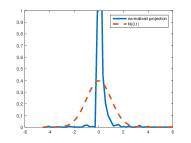
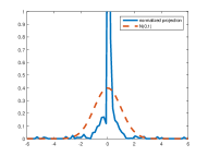
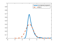
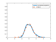
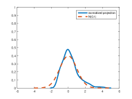
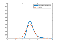
Figure 1: Plots of the kernel density estimates of the normalized estimates (blue) v.s. $N(0,1)$ (red) under the first projection direction ($n=100,200,400$ from top to bottom).

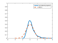
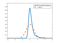
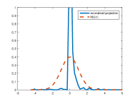
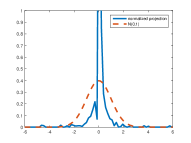
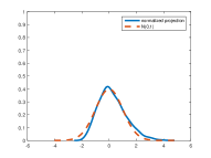
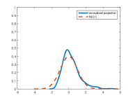
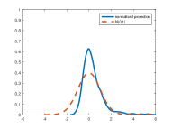
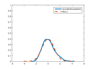
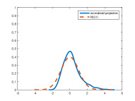
Figure 2: Plots of the kernel density estimates of the normalized estimates (blue) v.s. $N(0,1)$ (red) under the second projection direction ($n=100,200,400$ from top to bottom).

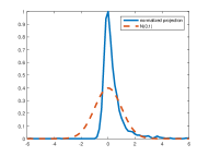
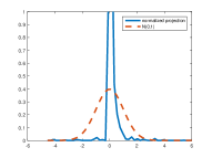
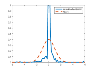
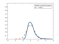
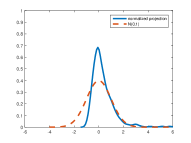
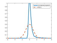
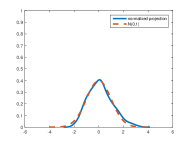
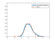
Figure 3: Plots of the kernel density estimates of the normalized estimates (blue) v.s. $N(0,1)$ (red) under the third projection direction ($n=100,200,400$ from top to bottom).

Based on 1,000 independent replications and using two-sided normal confidence interval, Tables 1-3 present the coverage probability as the nominal one varies from 0.5 to 0.95 for three projections of the same directions as $(1,1,\ldots,1)^{\top}$, $(1,0,\ldots,0)^{\top}$, and $(1,2,\ldots,p_{n})^{\top}$. For calculating the confidence intervals, we used the sample standard deviation of 1,000 replications. We further plot the kernel estimates of the density functions of the normalized three projected estimates against the density function of $N(0,1)$ in Figures 1-3. The normalization is based on the true mean and the previous simulation-based standard deviation. In computing the kernel density estimates, we used normal kernel function and the bandwidth based on Silverman’s rule-of-thumb.

Both the tables and figures reveal the same overall pattern that, for each fixed $n$, as $p_{n}$ increases, the coverage probability will deviate more from the nominal, and the kernel estimates of the density function of the normalized estimator itself will deviate more from the standard normal. As observed, the deviation from normal has become very severe even for very small $p_{n}$. For example, for $p_{n}=2$, we need $n$ to be approximately 400 for achieving satisfactory coverage probability. This supports the theoretical observations in Theorem 2.4 and Corollary 3.1(iii). We further conduct different types of normality tests (Kolmogorov-Smirnov, Lilliefors, Jarque-Bera, Anderson-Darling, Henze-Zirkler) on the derived projected estimates as well as the original multi-dimensional estimates. They all reject the null hypothesis of normality except when $p_{n}=1,n=400$.

We then move on to study the estimation accuracy of the asymptotic covariance estimator discussed at the end of Section 2.2. For this, we focus on the same setup as previously conducted. Table 4 presents the MAE of the asymptotic covariance estimator for the projection direction $\{p_{n}^{-1/2},\ldots,p_{n}^{-1/2}\}^{\top}$. There, it could be observed that, for each fixed $n$, the tuning parameter that attains the smallest MAE will in general become larger as $p_{n}$ increases, supporting our observation in Theorem 2.6 and Corollary 3.1(iv).

Concluding Remarks

This paper provided a first study of asymptotic properties of a general class of estimators defined as minimizers of possibly discontinuous objective functions of U-process structure allowing for the dimension of the parameter vector of interest to increase to infinity as the sample size $n$ increases to infinity. Members of this class include important rank correlation estimators as detailed throughout this paper. Technically we have established a maximal inequality for degenerate U-processes in increasing dimensions which has played a critical role in deriving our theoretical results. We have also applied our general theory to the four motivating rank correlation estimators. Using Han’s MRC estimator of the form (1.3), we have provided numerical support to our theoretical findings that for a given sample size, the accuracy of the normal approximation deteriorates quickly as the number of parameters $p_{n}$ increases and that for the variance estimation, the step size needs to be adjusted with respect to $p_{n}$.

This paper is focused on the setting that the parameter of interest itself is of an increasing dimension and inference has to be drawn on it. On the contrary, a growing literature studies the case that the parameter to be inferred is of a fixed dimension, but allows for a dimension-increasing (but still less than $n$) nuisance in the model. Substantial developments have been made along this line. For example, Cattaneo et al., 2018a and Cattaneo et al., 2018b studied inferring the fixed-dimension linear component in a partially linear model, and Lei et al., (2018) established asymptotic normality of margins of linear and robust regression estimators in a simple linear model. Their set-up is fundamentally different from ours due to the difference of goals.

We end this section with a brief discussion on further extensions. An immediate extension is on studying “penalized” rank estimators in ultra high dimensional settings where the dimension could be even larger than the sample size. For this much more challenging setting, to the authors’ knowledge, most literature is still focused on simple structural statistical models (cf. Zhang and Zhang, (2014), Van de Geer et al., (2014), Lee et al., (2016), and Javanmard and Montanari, (2018) among many others). A notable exception is the post-selection inference framework proposed in Belloni et al., (2014) and Belloni et al., (2018), where a general set of regularization conditions has been posed for inference validity of Z-estimation. The authors believe that, combined with our local entropy analysis of the degenerate U-processes and the empirical process techniques developed by Talagrand and Spokoiny and specialized to rank estimators in this paper, the post-selection inference framework will prove useful in extending the current study to ultra high dimensional models. However, there are still many technical gaps, which we believe are fundamental and related to some key challenges in high dimensional probability in extending the scalar empirical processes to vector and matrix ones if no further smoothing (cf. Han et al., (2017)) is made. We will leave this for future research.

Appendix A Appendix

A.1 Additional Notation

For a vector $\bm{\alpha}\in{{\mathbb{R}}}^{l}$, we define $|\bm{\alpha}|=(|\alpha_{1}|,\ldots,|\alpha_{l}|)^{\top}$. For two sequences of real numbers $a_{n}$ and $b_{n}$, $a_{n}\lesssim b_{n}$ means that $a_{n}\leq b_{n}$ up to a multiplicative constant. We use the symbol $a_{n}\sim b_{n}$ to denote that $a_{n}\lesssim b_{n}$ and $b_{n}\lesssim a_{n}$. In this appendix we drop the subscript $n$ in $m_{n},\nu_{n},p_{n}$.

A.2 Notation and Assumptions in Section 3

Throughout this section, let $\bm{X}=(X_{1},\widetilde{\bm{X}}^{\top})^{\top}$, where $\widetilde{\bm{X}}$ denotes the last $p$ components in $\bm{X}$.

A.2.1 Notation and Assumptions in Section 3.2

The following definitions are similar to those in Section 1.2. We use $S^{\mathsf{C}}(\bm{\beta})$ to denote the expected value of $S_{n}^{\mathsf{C}}(\bm{\beta})$, and $S^{\mathsf{C}}(\bm{\beta})=\mathbb{E}\{M(Y_{1})\mathds{1}(\bm{X}_{1}^{\top}\bm{\beta}>\bm{X}_{2}^{\top}\bm{\beta})\}$. Let $\bm{z}=(y,\bm{x}^{\top})^{\top}$. We define

$$f^{\mathsf{C}}(\bm{z}_{1},\bm{z}_{2};\bm{\theta})=M(y_{1})\{\mathds{1}(\bm{x}_{1}^{\top}\bm{\beta}>\bm{x}_{2}^{\top}\bm{\beta})-\mathds{1}(\bm{x}_{1}^{\top}\bm{\beta}_{0}>\bm{x}_{2}^{\top}\bm{\beta}_{0})\},$$

$$\tau^{\mathsf{C}}(\bm{z};\bm{\theta})=\mathbb{E}f^{\mathsf{C}}(\bm{z},\cdot;\bm{\theta})+\mathbb{E}f^{\mathsf{C}}(\cdot,\bm{z};\bm{\theta}),~{}~{}\zeta^{\mathsf{C}}(\bm{z};\bm{\theta})=\tau^{\mathsf{C}}(\bm{z};\bm{\theta})-\mathbb{E}\tau^{\mathsf{C}}(\cdot;\bm{\theta}),$$

$$\bm{\Delta}^{\mathsf{C}}=\mathbb{E}\nabla_{1}\tau^{\mathsf{C}}(\cdot;\bm{\theta}_{0})\{\nabla_{1}\tau^{\mathsf{C}}(\cdot;\bm{\theta}_{0})\}^{\top},~{}\mathrm{and}~{}2\mathbf{V}^{\mathsf{C}}=\mathbb{E}\nabla_{2}\tau^{\mathsf{C}}(\cdot;\bm{\theta}_{0}).$$

Write $\Gamma^{\mathsf{C}}(\bm{\theta})$ for $S^{\mathsf{C}}(\bm{\beta})-S^{\mathsf{C}}(\bm{\beta}_{0})$ and $\Gamma^{\mathsf{C}}_{n}(\bm{\theta})$ for $S^{\mathsf{C}}_{n}(\bm{\beta})-S^{\mathsf{C}}_{n}(\bm{\beta}_{0})$. The estimator $\widehat{\bm{\theta}}^{\mathsf{C}}_{n}$ is defined as

$$\widehat{\bm{\theta}}^{\mathsf{C}}_{n}=\mathop{\mathrm{argmax}}_{\bm{\theta}\in\Theta^{\mathsf{C}}}\Gamma^{\mathsf{C}}_{n}(\bm{\theta}).$$

To conduct inference on $\bm{\theta}_{0}$ based on $\widehat{\bm{\theta}}_{n}^{\mathsf{C}}$, we further define

$$\tau_{n}^{\mathsf{C}}(\bm{z};\bm{\theta})=\mathbb{P}_{n}f^{\mathsf{C}}(\bm{z},\cdot;\bm{\theta})+\mathbb{P}_{n}f^{\mathsf{C}}(\cdot,\bm{z};\bm{\theta}),~{}~{}p_{ni}^{\mathsf{C}}(\bm{z};\bm{\theta})=\varepsilon_{n}^{-1}\{\tau_{n}^{\mathsf{C}}(\bm{z};\bm{\theta}+\varepsilon_{n}\bm{u}_{i})-\tau_{n}^{\mathsf{C}}(\bm{z};\bm{\theta})\},~{}~{}\mathrm{and}~{}~{}$$

$$p_{nij}^{\mathsf{C}}(\bm{z};\bm{\theta})=\varepsilon_{n}^{-2}\{\tau_{n}^{\mathsf{C}}(\bm{z};\bm{\theta}+\varepsilon_{n}(\bm{u}_{i}+\bm{u}_{j}))-\tau_{n}^{\mathsf{C}}(\bm{z};\bm{\theta}+\varepsilon_{n}\bm{u}_{i})-\tau_{n}^{\mathsf{C}}(\bm{z};\bm{\theta}+\varepsilon_{n}\bm{u}_{j})+\tau_{n}^{\mathsf{C}}(\bm{z};\bm{\theta})\}.$$

Then, we define the estimator of the matrix $\bm{\Delta}^{\mathsf{C}}$ as $\widehat{\bm{\Delta}}^{\mathsf{C}}=(\widehat{\delta}_{ij}^{\mathsf{C}})$ and the estimator of the matrix $\mathbf{V}^{\mathsf{C}}$ as $\widehat{\mathbf{V}}^{\mathsf{C}}=(\widehat{v}_{ij}^{\mathsf{C}})$, where

$$\widehat{\delta}_{ij}^{\mathsf{C}}=\mathbb{P}_{n}\{p_{ni}^{\mathsf{C}}(\cdot;\widehat{\bm{\theta}}_{n}^{\mathsf{C}})p_{nj}^{\mathsf{C}}(\cdot;\widehat{\bm{\theta}}_{n}^{\mathsf{C}})\},~{}~{}\mathrm{and}~{}~{}\widehat{v}_{ij}^{\mathsf{C}}=\frac{1}{2}\mathbb{P}_{n}p_{nij}^{\mathsf{C}}(\cdot;\widehat{\bm{\theta}}_{n}^{\mathsf{C}}).$$

We then make the following assumptions.

Assumption 7.

Assume

1. Assumption 1 holds for $\Theta^{\mathsf{C}}$ and $\Gamma^{\mathsf{C}}(\bm{\theta})$.

2. The random variables $\bm{X}$ and $\epsilon$ are independent, and $\mathbb{E}\{M(Y)\mid\bm{X}\}$ depends on $\bm{X}$ only through $\bm{X}^{\top}\bm{\beta}_{0}$.

3. $X_{1}$ has an everywhere positive Lebesgue density, conditional on $\widetilde{\bm{X}}$.

4. Assumption 3 holds for $\tau^{\mathsf{C}}(\bm{z};\bm{\theta})$ and $\zeta^{\mathsf{C}}(\bm{z};\bm{\theta})$.

A.2.2 Notation and Assumptions in Section 3.3

The following definitions are similar to those in Section 1.2. Let $S^{\mathsf{K}}(\bm{\beta})$ denote the expected value of $S^{\mathsf{K}}_{n}(\bm{\beta})$, and $S^{\mathsf{K}}(\bm{\beta})=\mathbb{E}\{R_{1}\mathds{1}(V_{1}<V_{2})\mathds{1}(\bm{X}_{1}^{\top}\bm{\beta}<\bm{X}_{2}^{\top}\bm{\beta})\}$. Let $\bm{z}=(r,v,\bm{x}^{\top})^{\top}$. We define

$$f^{\mathsf{K}}(\bm{z}_{1},\bm{z}_{2};\bm{\theta})=r_{1}\mathds{1}(v_{1}<v_{2})\{\mathds{1}(\bm{x}_{1}^{\top}\bm{\beta}<\bm{x}_{2}^{\top}\bm{\beta})-\mathds{1}(\bm{x}_{1}^{\top}\bm{\beta}_{0}<\bm{x}_{2}^{\top}\bm{\beta}_{0})\},$$

$$\tau^{\mathsf{K}}(\bm{z};\bm{\theta})=\mathbb{E}f^{\mathsf{K}}(\bm{z},\cdot;\bm{\theta})+\mathbb{E}f^{\mathsf{K}}(\cdot,\bm{z};\bm{\theta}),~{}~{}\zeta^{\mathsf{K}}(\bm{z};\bm{\theta})=\tau^{\mathsf{K}}(\bm{z};\bm{\theta})-\mathbb{E}\tau^{\mathsf{K}}(\cdot;\bm{\theta}),$$

$$\bm{\Delta}^{\mathsf{K}}=\mathbb{E}\nabla_{1}\tau^{\mathsf{K}}(\cdot;\bm{\theta}_{0})\{\nabla_{1}\tau^{\mathsf{K}}(\cdot;\bm{\theta}_{0})\}^{\top},~{}~{}\mathrm{and}~{}~{}2\mathbf{V}^{\mathsf{K}}=\mathbb{E}\nabla_{2}\tau^{\mathsf{K}}(\cdot;\bm{\theta}_{0}).$$

Write $\Gamma^{\mathsf{K}}(\bm{\theta})$ for $S^{\mathsf{K}}(\bm{\beta})-S^{\mathsf{K}}(\bm{\beta}_{0})$ and $\Gamma^{\mathsf{K}}_{n}(\bm{\theta})$ for $S^{\mathsf{K}}_{n}(\bm{\beta})-S^{\mathsf{K}}_{n}(\bm{\beta}_{0})$. The estimator $\widehat{\bm{\theta}}^{\mathsf{K}}_{n}$ is defined as

$$\widehat{\bm{\theta}}^{\mathsf{K}}_{n}=\mathop{\mathrm{argmax}}_{\bm{\theta}\in\Theta^{\mathsf{K}}}\Gamma^{\mathsf{K}}_{n}(\bm{\theta}).$$

To conduct inference on $\bm{\theta}_{0}$ based on $\widehat{\bm{\theta}}_{n}^{\mathsf{K}}$, we further define

$$\tau_{n}^{\mathsf{K}}(\bm{z};\bm{\theta})=\mathbb{P}_{n}f^{\mathsf{K}}(\bm{z},\cdot;\bm{\theta})+\mathbb{P}_{n}f^{\mathsf{K}}(\cdot,\bm{z};\bm{\theta}),~{}~{}p_{ni}^{\mathsf{K}}(\bm{z};\bm{\theta})=\varepsilon_{n}^{-1}\{\tau_{n}^{\mathsf{K}}(\bm{z};\bm{\theta}+\varepsilon_{n}\bm{u}_{i})-\tau_{n}^{\mathsf{K}}(\bm{z};\bm{\theta})\},~{}~{}\mathrm{and}~{}~{}$$

$$p_{nij}^{\mathsf{K}}(\bm{z};\bm{\theta})=\varepsilon_{n}^{-2}\{\tau_{n}^{\mathsf{K}}(\bm{z};\bm{\theta}+\varepsilon_{n}(\bm{u}_{i}+\bm{u}_{j}))-\tau_{n}^{\mathsf{K}}(\bm{z};\bm{\theta}+\varepsilon_{n}\bm{u}_{i})-\tau_{n}^{\mathsf{K}}(\bm{z};\bm{\theta}+\varepsilon_{n}\bm{u}_{j})+\tau_{n}^{\mathsf{K}}(\bm{z};\bm{\theta})\}.$$

Then, we define the estimator of the matrix $\bm{\Delta}^{\mathsf{K}}$ as $\widehat{\bm{\Delta}}^{\mathsf{K}}=(\widehat{\delta}_{ij}^{\mathsf{K}})$ and the estimator of the matrix $\mathbf{V}^{\mathsf{K}}$ as $\widehat{\mathbf{V}}^{\mathsf{K}}=(\widehat{v}_{ij}^{\mathsf{K}})$, where

$$\widehat{\delta}_{ij}^{\mathsf{K}}=\mathbb{P}_{n}\{p_{ni}^{\mathsf{K}}(\cdot;\widehat{\bm{\theta}}_{n}^{\mathsf{K}})p_{nj}^{\mathsf{K}}(\cdot;\widehat{\bm{\theta}}_{n}^{\mathsf{K}})\}~{}~{}\mathrm{and}~{}~{}\widehat{v}_{ij}^{\mathsf{K}}=\frac{1}{2}\mathbb{P}_{n}p_{nij}^{\mathsf{K}}(\cdot;\widehat{\bm{\theta}}_{n}^{\mathsf{K}}).$$

We then make the following assumptions.

Assumption 8.

Assume

1. Assumption 1 holds for $\Theta^{\mathsf{K}}$ and $\Gamma^{\mathsf{K}}(\bm{\theta})$.

2. The random variables $(\xi,\bm{X})$ and $\epsilon$ are independent, and $\mathbb{E}(\xi\mid\bm{X})$ depends on $\bm{X}$ only through $\bm{X}^{\top}\bm{\beta}_{0}$.

3. $X_{1}$ has an everywhere positive Lebesgue density, conditional on $\widetilde{\bm{X}}$.

4. Assumption 3 holds for $\tau^{\mathsf{K}}(\bm{z};\bm{\theta})$ and $\zeta^{\mathsf{K}}(\bm{z};\bm{\theta})$.

A.2.3 Notation and Assumptions in Section 3.4

Let $\phi(\cdot)$ denote the density of $W$. Let $\bm{z}=(y,\bm{x}^{\top},w)^{\top}$. We define

$$f^{\mathsf{A}}(\bm{z}_{1},\bm{z}_{2};\bm{\theta})=\mathds{1}(y_{1}>y_{2})\{\mathds{1}(\bm{x}_{1}^{\top}\bm{\beta}>\bm{x}_{2}^{\top}\bm{\beta})-\mathds{1}(\bm{x}_{1}^{\top}\bm{\beta}_{0}>\bm{x}_{2}^{\top}\bm{\beta}_{0})\}K\{(w_{1}-w_{2})/b\},$$

$$m(\bm{z}_{1},\bm{z}_{2};\bm{\theta})=\mathds{1}(y_{1}>y_{2})\mathds{1}(\bm{x}_{1}^{\top}\bm{\beta}>\bm{x}_{2}^{\top}\bm{\beta}),$$

$$\psi(w_{1},w_{2};\bm{\theta})=\mathbb{E}\{m(\bm{Z}_{1},\bm{Z}_{2};\bm{\theta})-m(\bm{Z}_{1},\bm{Z}_{2};\bm{\theta}_{0})\mid W_{1}=w_{1},W_{2}=w_{2}\},$$

$$\Gamma^{\mathsf{A}}(\bm{\theta})=\mathbb{E}_{W}\{\psi(W,W;\bm{\theta})\phi(W)\},$$

$$\tau^{\mathsf{A}}(\bm{z};\theta)=\mathbb{E}\{m(\bm{z},\bm{Z}_{2};\bm{\theta})\mid W_{2}=w\}\phi(w)+\mathbb{E}\{m(\bm{Z}_{1},\bm{z};\bm{\theta})\mid W_{1}=w\}\phi(w),$$

$$\zeta^{\mathsf{A}}(\bm{z};\bm{\theta})=\tau^{\mathsf{A}}(\bm{z};\bm{\theta})-\mathbb{E}\tau^{\mathsf{A}}(\cdot;\bm{\theta}),~{}~{}\bm{\Delta}^{\mathsf{A}}=\mathbb{E}\nabla_{1}\tau^{\mathsf{A}}(\cdot;\bm{\theta}_{0})\{\nabla_{1}\tau^{\mathsf{A}}(\cdot;\bm{\theta}_{0})\}^{\top},~{}~{}\mathrm{and}~{}~{}2\mathbf{V}^{\mathsf{A}}=\mathbb{E}\nabla_{2}\tau^{\mathsf{A}}(\cdot;\bm{\theta}_{0}).$$

Write $\Gamma_{n}^{\mathsf{A}}(\bm{\theta})$ for $S_{n}^{\mathsf{A}}(\bm{\beta})-S_{n}^{\mathsf{A}}(\bm{\beta}_{0})$. The estimator $\widehat{\bm{\theta}}^{\mathsf{A}}_{n}$ is defined as

$$\widehat{\bm{\theta}}^{\mathsf{A}}_{n}=\mathop{\mathrm{argmax}}_{\bm{\theta}\in\Theta^{\mathsf{A}}}\Gamma^{\mathsf{A}}_{n}(\bm{\theta}).$$

Note that $\mathbb{E}\Gamma_{n}^{\mathsf{A}}(\bm{\theta})\neq\Gamma^{\mathsf{A}}(\bm{\theta})$. This is different from the general set-up in Section 2.2. However, by Taylor expansion, we show that $\sup_{\bm{\theta}\in\Theta^{\mathsf{A}}}\big{|}\mathbb{E}\Gamma_{n}^{\mathsf{A}}(\bm{\theta})-\Gamma^{\mathsf{A}}(\bm{\theta})\big{|}$ is negligible under the assumptions adopted in this section. Then, following the proof of the general method, we can similarly establish the consistency and asymptotic normality of $\widehat{\bm{\theta}}_{n}^{\mathsf{A}}$.

To conduct inference on $\bm{\theta}_{0}$ based on $\widehat{\bm{\theta}}_{n}^{\mathsf{A}}$, we further define

$$\tau_{n}^{\mathsf{A}}(\bm{z};\bm{\theta})=\mathbb{P}_{n}f^{\mathsf{A}}(\bm{z},\cdot;\bm{\theta})+\mathbb{P}_{n}f^{\mathsf{A}}(\cdot,\bm{z};\bm{\theta}),~{}~{}p_{ni}^{\mathsf{A}}(\bm{z};\bm{\theta})=\varepsilon_{n}^{-1}\{\tau_{n}^{\mathsf{A}}(\bm{z};\bm{\theta}+\varepsilon_{n}\bm{u}_{i})-\tau_{n}^{\mathsf{A}}(\bm{z};\bm{\theta})\},~{}~{}\mathrm{and}~{}~{}$$

$$p_{nij}^{\mathsf{A}}(\bm{z};\bm{\theta})=\varepsilon_{n}^{-2}\{\tau_{n}^{\mathsf{A}}(\bm{z};\bm{\theta}+\varepsilon_{n}(\bm{u}_{i}+\bm{u}_{j}))-\tau_{n}^{\mathsf{A}}(\bm{z};\bm{\theta}+\varepsilon_{n}\bm{u}_{i})-\tau_{n}^{\mathsf{A}}(\bm{z};\bm{\theta}+\varepsilon_{n}\bm{u}_{j})+\tau_{n}^{\mathsf{A}}(\bm{z};\bm{\theta})\}.$$

Then, we define the estimator of the matrix $\bm{\Delta}^{\mathsf{A}}$ as $\widehat{\bm{\Delta}}^{\mathsf{A}}=(\widehat{\delta}_{ij}^{\mathsf{A}})$ and the estimator of the matrix $\mathbf{V}^{\mathsf{A}}$ as $\widehat{\mathbf{V}}^{\mathsf{A}}=(\widehat{v}_{ij}^{\mathsf{A}})$, where

$$\widehat{\delta}_{ij}^{\mathsf{A}}=\mathbb{P}_{n}\{p_{ni}^{\mathsf{A}}(\cdot;\widehat{\bm{\theta}}_{n}^{\mathsf{A}})p_{nj}^{\mathsf{A}}(\cdot;\widehat{\bm{\theta}}_{n}^{\mathsf{A}})\},~{}~{}\mathrm{and}~{}~{}\widehat{v}_{ij}^{\mathsf{A}}=\frac{1}{2}\mathbb{P}_{n}p_{nij}^{\mathsf{A}}(\cdot;\widehat{\bm{\theta}}_{n}^{\mathsf{A}}).$$

We make the following assumptions.

Assumption 9.

Assume

1. Assumption 1 holds for $\Theta^{\mathsf{A}}$ and $\Gamma^{\mathsf{A}}(\bm{\theta})$;

2. The random variables $(\bm{X},W)$ and $\epsilon$ are independent.

3. $X_{1}$ has an everywhere positive Lebesgue density, conditional on $\widetilde{\bm{X}}$ and $W$.

4. $W$ is continuously distributed on a compact subset $\mathcal{W}$ of ${{\mathbb{R}}}$.

5. The kernel function $K(\cdot)$ satisfies: (1) $K(\cdot)$ is twice continuously differential with compact interval $[-C,C]\supseteq\mathcal{W}$; (2) $K(\cdot)$ is symmetric about 0 and integrates to 1; (3) for some integer $J\geq 6$, $\int u^{j}K(u)\mathop{}\!\mathrm{d}u=0$ with $j=1,\ldots,J-1$ and $\int u^{J}K(u)\mathop{}\!\mathrm{d}u$ is bounded.

6. The bandwidth $b$ is defined as $b=cn^{-\delta}$ for constants $c>0$ and $\frac{1}{J}<\delta<\frac{1}{5}$.

7. For any $w_{2}$, the $J$th derivative of $\psi(w_{1},w_{2};\bm{\theta})\cdot\phi(w_{1})$ with respect to $w_{1}$ is continuous and bounded for all $\bm{\theta}\in\Theta^{\mathsf{A}}$.

8. Assumption 3 holds for $\tau^{\mathsf{A}}(\bm{z};\bm{\theta})$ and $\zeta^{\mathsf{A}}(\bm{z};\bm{\theta})$.

Assumption 10.

Let $f_{0}(\cdot\mid\widetilde{\bm{x}},w)$ denote the conditional density function of $\bm{X}^{\top}\bm{\beta}_{0}$ given $(\widetilde{\bm{X}},W)=(\widetilde{\bm{x}},w)$. Assume $f_{0}(\cdot\mid\widetilde{\bm{x}},w)\leq C_{1}$ for any $\widetilde{\bm{x}}$ and $w$ in the support of $\widetilde{\bm{X}}$ and $W$, respectively, where $C_{1}$ is an absolute positive constant.

A.3 Proofs in Section 2

For each $\bm{\theta}\in\Theta$, define measures

$$\mathbb{S}_{n}f(\cdot,\cdot;\bm{\theta})=n(n-1)\mathbb{U}_{n}f(\cdot,\cdot;\bm{\theta})$$

and

$$\mathbb{T}_{n}f(\cdot,\cdot;\bm{\theta})=\sum_{i\neq j}\{f(\bm{Z}_{2i},\bm{Z}_{2j};\newline \bm{\theta})+f(\bm{Z}_{2i},\bm{Z}_{2j-1};\bm{\theta})+f(\bm{Z}_{2i-1},\bm{Z}_{2j};\bm{\theta})+f(\bm{Z}_{2i-1},\bm{Z}_{2j-1};\bm{\theta})\}.$$

To prove Theorems 2.1–2.4 in Section 2, we need several lemmas. For simplicity, we omit the parameter $\bm{\theta}$ in each function $f(\cdot,\cdot;\bm{\theta})\in\mathcal{F}$ in the lemmas. Let $F$ denote the envelope function of $\mathcal{F}$ for which $0<\mathbb{E}F^{r}<\infty$, for any $r\geq 1$. The covering number $N_{r}(\varepsilon,\mathbb{P}\otimes\mathbb{P},\mathcal{F},F)$ is defined as the smallest cardinality for a subclass $\mathcal{F}^{*}$ of $\mathcal{F}$ such that $\min_{f^{*}\in\mathcal{F}^{*}}\mathbb{E}|f-f^{*}|^{r}\leq\varepsilon^{r}\mathbb{E}F^{r}$, for each $f\in\mathcal{F}$.

A.3.1 Some Auxiliary Lemmas

Lemma A.1.

Suppose that $\mathcal{F}$ is $b$-uniformly bounded, then the class $\mathcal{F}^{2}=\{f^{2}:f\in\mathcal{F}\}$ with envelope $b^{2}$ satisfies $N_{r}(2\varepsilon,\mathbb{P}\otimes\mathbb{P},\mathcal{F}^{2},b^{2})\leq N_{r}(\varepsilon,\mathbb{P}\otimes\mathbb{P},\mathcal{F},b)$.

Proof.

Find functions $f_{1},\ldots,f_{m}$ such that

$$\min_{i}\mathbb{E}|f-f_{i}|^{r}\leq\varepsilon^{r}b^{r},\quad\text{for each $f\in\mathcal{F}$.}$$

Then, with the appropriate $i$,

$$\mathbb{E}|f^{2}-f^{2}_{i}|^{r}\leq(2b)^{r}\mathbb{E}|f-f_{i}|^{r}\leq(2b)^{r}\varepsilon^{r}b^{r}=(2\epsilon)^{r}(b^{2})^{r}.$$

This implies that $N_{r}(2\varepsilon,\mathbb{P}\otimes\mathbb{P},\mathcal{F}^{2},b^{2})\leq N_{r}(\varepsilon,\mathbb{P}\otimes\mathbb{P},\mathcal{F},b)$. ∎

Lemma A.2.

Suppose that $\mathcal{F}$ is $b$-uniformly bounded. Then $\mathbb{E}\sup_{g\in\mathbb{P}\mathcal{F}}|\mathbb{P}_{n}g-\mathbb{E}g|\lesssim\sqrt{\nu/n}$, where $\mathbb{P}\mathcal{F}:=\{\mathbb{E}_{\mathbb{P}}f(\bm{z},\cdot):f\in\mathcal{F}\}$.

Proof.

With a little abuse of notation, let $\epsilon_{1},\epsilon_{2},\cdots$ be the Rademacher sequence, where $\epsilon_{i}\in\{-1,1\}$ is symmetric around 0. By the classic symmetrization theorem (cf. Theorem 8.8 in Kosorok,, 2007), we have

$$\mathbb{E}\sup_{g\in\mathbb{P}\mathcal{F}}|\mathbb{P}_{n}g-\mathbb{E}g|\leq\mathbb{E}_{\bm{Z}}\mathbb{E}_{\epsilon}\sup_{g\in\mathbb{P}\mathcal{F}}\Big{|}\frac{1}{n}\sum_{i=1}^{n}\epsilon_{i}g(\bm{Z}_{i})\Big{|}.$$ (A.1)

Next, we try to bound $\mathbb{E}_{\epsilon}\sup_{g\in\mathbb{P}\mathcal{F}}|\sum_{i=1}^{n}\epsilon_{i}g(\bm{z}_{i})/n|$ for fixed $\bm{z}_{i}$. To that end, consider the stochastic process $\{\sum_{i=1}^{n}\epsilon_{i}g(\bm{z}_{i})/\sqrt{n}:g\in\mathbb{P}\mathcal{F}\}$. It is easy to verify that $\sum_{i=1}^{n}\epsilon_{i}\{g_{1}(\bm{z}_{i})-g_{2}(\bm{z}_{i})\}/\sqrt{n}$ is sub-gaussian with parameter $\|g_{1}-g_{2}\|^{2}_{L_{2}(\mathbb{P}_{n})}:=\sum_{i=1}^{n}\{g_{1}(\bm{z}_{i})-g_{2}(\bm{z}_{i})\}^{2}/n$, where $g_{1},g_{2}\in\mathbb{P}\mathcal{F}$. Consequently, Dudley’s entropy integral, combined with the fact that $\sup_{g_{1},g_{2}\in\mathbb{P}\mathcal{F}}\|g_{1}-g_{2}\|_{L_{2}(\mathbb{P}_{n})}\leq 2b$, implies that

$$\mathbb{E}_{\epsilon}\sup_{g\in\mathbb{P}\mathcal{F}}\Big{|}\frac{1}{n}\sum_{i=1}^{n}\epsilon_{i}g(\bm{z}_{i})\Big{|}\leq\frac{24}{\sqrt{n}}\int_{0}^{2b}\sqrt{\log N_{2}(t/b,\mathbb{P}_{n},\mathbb{P}\mathcal{F},b)}\mathop{}\!\mathrm{d}t.$$ (A.2)

By Theorem 9.3 in Kosorok, (2007) and Lemma 20 in Nolan and Pollard, (1987), there exists a universal constant $K$ such that $N_{2}(t/b,\mathbb{P}_{n},\mathbb{P}\mathcal{F},b)\leq K\nu(16e)^{\nu}(b/t)^{2(\nu-1)}$. Substituting this bound into (A.2), we find that there exist constants $c_{0},c_{1}$, only depending on $K,b$ but not on $(\nu,n)$, such that

$$\mathbb{E}_{\epsilon}\sup_{g\in\mathbb{P}\mathcal{F}}\Big{|}\frac{1}{n}\sum_{i=1}^{n}\epsilon_{i}g(\bm{z}_{i})\Big{|}\leq c_{0}\sqrt{\frac{\nu}{n}}\left\{1+\int_{0}^{2b}\sqrt{\log(b/t)}\mathop{}\!\mathrm{d}t\right\}\leq c_{1}\sqrt{\frac{\nu}{n}}.$$

Combining this with (A.1) implies that $\mathbb{E}\sup_{g\in\mathbb{P}\mathcal{F}}|\mathbb{P}_{n}g-\mathbb{E}g|\leq c_{1}\sqrt{\nu/n}$. This completes the proof. ∎

Lemma A.3.

Suppose that $\mathcal{F}$ is $\mathbb{P}$-degenerate and $b$-uniformly bounded. Then $\mathbb{E}\sup_{f\in\mathcal{F}}|\mathbb{U}_{n}f|\lesssim\nu/n$.

Proof.

First, by the relationship between $\mathbb{S}_{n}$ and $\mathbb{U}_{n}$: $\mathbb{S}_{n}=n(n-1)\mathbb{U}_{n}$, we just need to show that $\mathbb{E}\sup_{f\in\mathcal{F}}|\mathbb{S}_{n}f/(n\nu)|$ is bounded. Apply Theorem 6 in Nolan and Pollard, (1987) to get

$$\mathbb{E}\sup_{f\in\mathcal{F}}|\mathbb{S}_{n}f|\leq C\mathbb{E}\bigg{\{}\sigma_{n}+\tau_{n}J_{n}\Big{(}\frac{\sigma_{n}}{\tau_{n}}\Big{)}\bigg{\}},$$ (A.3)

where $C$ is a universal constant, $\sigma_{n}=\sup_{f\in\mathcal{F}}(\mathbb{T}_{n}f^{2})^{1/2}/4$, $\tau_{n}=(\mathbb{T}_{n}b^{2})^{1/2}$, and $J_{n}(x)=\int_{0}^{x}\log N_{2}(t,\\ \mathbb{T}_{n},\mathcal{F},b)\mathop{}\!\mathrm{d}t$. By Theorem 9.3 in Kosorok, (2007), we have $N_{2}(t,\mathbb{T}_{n},\mathcal{F},1)\leq K\nu(4e)^{\nu}(2/t)^{2(\nu-1)}$, and thus $J_{n}(x)\leq cH(x)\nu$ for some constant $c$ depending on $K$, where $H(x)=x\{1+\log(1/x)\}$.

Since $\mathcal{F}$ is $b$-uniformly bounded, it holds that $\sigma_{n}/\tau_{n}\in[0,1/4]$. Note also that $H(x)$ is bounded when $x\in[0,1]$. We immediately have $H(\sigma_{n}/\tau_{n})$ is bounded. Additionally, by the definition of $\mathbb{T}_{n}$, we see that $\tau_{n}=\{4n(n-1)\}^{1/2}\lesssim n$. Combining all these points with (A.3) implies that there exists some constant $c^{\prime}$ depending on $C,c$ such that

$$\frac{\mathbb{E}\sup_{f\in\mathcal{F}}|\mathbb{S}_{n}f|}{nv}\leq c^{\prime}\mathbb{E}H\Big{(}\frac{\sigma_{n}}{\tau_{n}}\Big{)}\frac{\tau_{n}}{n}<C^{\prime}$$

for some large enough absolute constant $C^{\prime}$. This completes the proof. ∎

Lemma A.4.

If for each $\varepsilon>0$, (i) $\log N_{1}(\varepsilon,\mathbb{T}_{n},\mathcal{F},F)=O_{\mathbb{P}}(n)$, (ii) $\log N_{1}(\varepsilon,\mathbb{P}_{n}\otimes\mathbb{P},\mathcal{F},F)=o_{\mathbb{P}}(n)$, (iii) $\log N_{1}(\varepsilon,\mathbb{P}\otimes\mathbb{P},\mathcal{F},F)=o(n)$, then $\sup_{f\in\mathcal{F}}|\mathbb{U}_{n}f-\mathbb{E}f|\rightarrow 0$ almost surely.

The proof of this lemma follows along the same lines as the proof of Theorem 7 in Nolan and Pollard, (1987), though the condition (iii) in this lemma is different from there.

A.3.2 Proof of Theorem 2.1

Proof.

(i) It is equivalent to showing that there exists a sequence of nonnegative real numbers $\delta_{n}$ converging to zero such that

$$\mathbb{P}\bigg{\{}\sup_{\bm{\theta}\in\overline{\mathcal{B}}(\bm{\theta}_{0},r_{n})}|\mathbb{U}_{n}h(\cdot,\cdot;\bm{\theta})|\geq\delta_{n}\nu/n\bigg{\}}=o(1),$$

or

$$\mathbb{P}\bigg{\{}\sup_{\bm{\theta}\in\overline{\mathcal{B}}(\bm{\theta}_{0},r_{n})}|\mathbb{S}_{n}h(\cdot,\cdot;\bm{\theta})/(n\nu)|\geq\delta_{n}\bigg{\}}=o(1).$$

By Chebyshev’s inequality, it suffices to show that

$$\mathbb{E}\Big{\{}\sup_{\bm{\theta}\in\overline{\mathcal{B}}(\bm{\theta}_{0},r_{n})}|\mathbb{S}_{n}h(\cdot,\cdot;\bm{\theta})/(n\nu)|\Big{\}}/\delta_{n}=o(1).$$

We try to bound $\mathbb{E}\{\sup_{\bm{\theta}\in\overline{\mathcal{B}}(\bm{\theta}_{0},r_{n})}|\mathbb{S}_{n}h(\cdot,\cdot;\bm{\theta})/(n\nu)|\}$. Without loss of generality, assume $\mathcal{F}$ is uniformly bounded by $b=1/4$. Thus, for any $\bm{\theta}\in\Theta$, $h(\cdot,\cdot;\bm{\theta})\leq 1$, i.e., the class of functions $\mathscr{H}:=\{h^{2}(\cdot,\cdot;\bm{\theta}):\bm{\theta}\in\overline{\mathcal{B}}(\bm{\theta}_{0},r_{n})\}$ is 1-uniformly bounded. Similar to the proof of Lemma A.3, we apply Theorem 6 in Nolan and Pollard, (1987) here to get

$$\mathbb{E}\Big{\{}\sup_{\bm{\theta}\in\overline{\mathcal{B}}(\bm{\theta}_{0},r_{n})}|\mathbb{S}_{n}h(\cdot,\cdot;\bm{\theta})/(n\nu)|\Big{\}} \leq C_{1}\mathbb{E}H\Big{(}\sup_{\bm{\theta}\in\overline{\mathcal{B}}(\bm{\theta}_{0},r_{n})}\{\mathbb{T}_{n}h^{2}(\cdot,\cdot;\bm{\theta})\}^{1/2}/(2n)\Big{)}$$ (A.4)

$$\leq C_{1}H\Big{(}\mathbb{E}\Big{[}\sup_{\bm{\theta}\in\overline{\mathcal{B}}(\bm{\theta}_{0},r_{n})}\{\mathbb{T}_{n}h^{2}(\cdot,\cdot;\bm{\theta})\}^{1/2}/(2n)\Big{]}\Big{)}$$

$$=C_{1}H\Big{(}\mathbb{E}\Big{\{}\sup_{\bm{\theta}\in\overline{\mathcal{B}}(\bm{\theta}_{0},r_{n})}\mathbb{T}_{n}h^{2}(\cdot,\cdot;\bm{\theta})/(2n)^{2}\Big{\}}^{1/2}\Big{)},$$

where $C_{1}$ is some constant. The second inequality holds because $H(x)$ is concave in $x$.

Note that $\mathbb{T}_{n}h^{2}(\cdot,\cdot;\bm{\theta})/(2n)^{2}=\mathbb{T}_{n}h^{2}(\cdot,\cdot;\bm{\theta})/\{2n(2n-1)\}\cdot\{2n(2n-1)\}/(2n)^{2}\leq\mathbb{U}_{2n}h^{2}(\cdot,\cdot;\bm{\theta})\leq 1$ and that $H(x)$ is increasing in $(0,1]$. Thus, from (A.4), we additionally have

$$\mathbb{E}\Big{\{}\sup_{\bm{\theta}\in\overline{\mathcal{B}}(\bm{\theta}_{0},r_{n})}|\mathbb{S}_{n}h(\cdot,\cdot;\bm{\theta})/(n\nu)|\Big{\}} \leq C_{1}H\Big{(}\mathbb{E}\Big{\{}\sup_{\bm{\theta}\in\overline{\mathcal{B}}(\bm{\theta}_{0},r_{n})}\mathbb{U}_{2n}h^{2}(\cdot,\cdot;\bm{\theta})\Big{\}}^{1/2}\Big{)}$$ (A.5)

$$\leq C_{1}H\Big{(}\Big{[}\mathbb{E}\Big{\{}\sup_{\bm{\theta}\in\overline{\mathcal{B}}(\bm{\theta}_{0},r_{n})}\mathbb{U}_{2n}h^{2}(\cdot,\cdot;\bm{\theta})\Big{\}}\Big{]}^{1/2}\Big{)},$$

where the last inequality holds because $x^{1/2}$ is concave in $x$. Now, we need only to consider $\mathbb{E}\{\sup_{\bm{\theta}\in\overline{\mathcal{B}}(\bm{\theta}_{0},r_{n})}\mathbb{U}_{2n}h^{2}(\cdot,\cdot;\bm{\theta})\}$.

By a decomposition of $\mathbb{U}_{2n}h^{2}(\cdot,\cdot,\bm{\theta})$ into a sum of its expected value, plus a smoothly parameterized, zero-mean empirical process, plus a degenerate $U$-process of order two, we have

$$\mathbb{E}\Big{\{}\sup_{\bm{\theta}\in\overline{\mathcal{B}}(\bm{\theta}_{0},r_{n})}\mathbb{U}_{2n}h^{2}(\cdot,\cdot;\bm{\theta})\Big{\}}\leq \sup_{\bm{\theta}\in\overline{\mathcal{B}}(\bm{\theta}_{0},r_{n})}\mathbb{E}h^{2}(\cdot,\cdot;\bm{\theta})+\mathbb{E}\Big{\{}\sup_{\bm{\theta}\in\overline{\mathcal{B}}(\bm{\theta}_{0},r_{n})}|\mathbb{P}_{2n}h_{1}(\cdot;\bm{\theta})|\Big{\}}$$ (A.6)

$$\hskip 10.00002pt+\mathbb{E}\Big{\{}\sup_{\bm{\theta}\in\overline{\mathcal{B}}(\bm{\theta}_{0},r_{n})}|\mathbb{P}_{2n}h_{2}(\cdot,\cdot;\bm{\theta})|\Big{\}},$$

where $h_{1}(\bm{z},\bm{\theta})=\mathbb{E}h^{2}(\bm{z},\cdot;\bm{\theta})+\mathbb{E}h^{2}(\cdot,\bm{z};\bm{\theta})-2\mathbb{E}h^{2}(\cdot,\cdot;\bm{\theta})$ and $h_{2}(\bm{z}_{1},\bm{z}_{2};\bm{\theta})=h^{2}(\bm{z}_{1},\bm{z}_{2};\bm{\theta})-\mathbb{E}h^{2}(\bm{z}_{1},\cdot;\bm{\theta})-\mathbb{E}h^{2}(\cdot,\bm{z}_{2};\bm{\theta})+\mathbb{E}h^{2}(\cdot,\cdot;\bm{\theta})$.

By the condition in (i), it holds that $\sup_{\bm{\theta}\in\overline{\mathcal{B}}(\bm{\theta}_{0},r_{n})}\mathbb{E}h^{2}(\cdot,\cdot;\bm{\theta})\leq\epsilon_{n}$. By Lemmas 16 and 20 in Nolan and Pollard, (1987), and Lemma A.1, we have $N_{r}(\varepsilon,\mathbb{Q},\mathscr{H},1)\leq N_{r}(\varepsilon/16,\mathbb{Q},\mathcal{F},1/4)^{4}$. Then, following the proof of Lemma A.2, we have $\mathbb{E}\{\sup_{\bm{\theta}\in\overline{\mathcal{B}}(\bm{\theta}_{0},r_{n})}|\mathbb{P}_{2n}h_{1}(\cdot;\bm{\theta})|\}\leq C_{2}\sqrt{\nu/n}$ for some constant $C_{2}$. Additionally, following the proof of Lemma A.3, we have $\mathbb{E}\{\sup_{\bm{\theta}\in\overline{\mathcal{B}}(\bm{\theta}_{0},r_{n})}|\mathbb{P}_{2n}h_{2}(\cdot,\cdot;\bm{\theta})|\}\leq C_{3}\nu/n$ for some constant $C_{3}$.

Take $\delta_{n}=H^{1/2}((\epsilon_{n}+C_{2}\sqrt{\nu/n}+C_{3}\nu/n)^{1/2})$. If $\epsilon_{n}\rightarrow 0$ and $\nu/n\rightarrow 0$, then

$$\mathbb{E}\Big{\{}\sup_{\bm{\theta}\in\overline{\mathcal{B}}(\bm{\theta}_{0},r_{n})}|\mathbb{S}_{n}h(\cdot,\cdot;\bm{\theta})/(n\nu)|\Big{\}}/\delta_{n}\leq C_{1}H^{1/2}((\epsilon_{n}+C_{2}\sqrt{\nu/n}+C_{3}\nu/n)^{1/2})=o(1),$$

because $H(x)\rightarrow 0$ as $x\rightarrow 0$. This completes proof of (i).

(ii) The proof is based on (A.4)–(A.6) in the proof of (i). First, by the condition in (ii), it holds that $\sup_{\bm{\theta}\in\overline{\mathcal{B}}(\bm{\theta}_{0},r_{n})}\mathbb{E}h^{2}(\cdot,\cdot;\bm{\theta})\leq\widetilde{\epsilon}_{n}$. Then, similar to the proof of (i), $\mathbb{E}\{\sup_{\bm{\theta}\in\overline{\mathcal{B}}(\bm{\theta}_{0},r_{n})}|\mathbb{P}_{2n}h_{1}(\cdot;\bm{\theta})|\}\leq c^{\prime}\sqrt{\nu/n}$ for some constant $c^{\prime}$, and $\mathbb{E}\{\sup_{\bm{\theta}\in\overline{\mathcal{B}}(\bm{\theta}_{0},r_{n})}|\mathbb{P}_{2n}h_{2}(\cdot,\cdot;\bm{\theta})|\}\leq C^{\prime}\nu/n$ for some constant $C^{\prime}$. Since $\widetilde{\eta}_{n}=\sqrt{\nu/n}\vee\widetilde{\epsilon}_{n}$ and $\nu/n\rightarrow 0$, there exists a constant $c^{\prime\prime}$ depending on $c^{\prime},C^{\prime}$ such that

$$\mathbb{E}\Big{\{}\sup_{\bm{\theta}\in\overline{\mathcal{B}}(\bm{\theta}_{0},r_{n})}\mathbb{U}_{2n}h^{2}(\cdot,\cdot;\bm{\theta})\Big{\}}\leq c^{\prime\prime}\widetilde{\eta}_{n}$$

holds for sufficiently large $n$. Combining this with (A.5) implies that

$$\mathbb{E}\Big{\{}\sup_{\bm{\theta}\in\overline{\mathcal{B}}(\bm{\theta}_{0},r_{n})}|\mathbb{S}_{n}h(\cdot,\cdot;\bm{\theta})/(n\nu)|\Big{\}}\leq C^{\prime\prime}\log(1/\widetilde{\eta}_{n})\widetilde{\eta}_{n}^{1/2}$$

for some constant $C^{\prime\prime}$. Finally, by the relationship between $\mathbb{U}_{n}$ and $\mathbb{S}_{n}$, we conclude that

$$\mathbb{E}\sup_{\bm{\theta}\in\overline{\mathcal{B}}(\bm{\theta}_{0},r_{n})}|\mathbb{U}_{n}h(\cdot,\cdot;\bm{\theta})|\leq C^{\prime\prime}\log(1/\widetilde{\eta}_{n})\widetilde{\eta}_{n}^{1/2}\nu/n$$

holds for sufficiently large $n$. ∎

A.3.3 Proof of Theorem 2.2

Proof.

The proof is twofold. We first show the uniform convergence of $\Gamma_{n}(\bm{\theta})$, and then establish the consistency of $\widehat{\bm{\theta}}_{n}$.

Step 1. By Theorem 9.3 in Kosorok, (2007), we have $\log N_{1}(\varepsilon,\mu,\mathcal{F},F)\lesssim\nu$ for any $\varepsilon>0$ and any finite measure $\mu$. If $\nu/n\rightarrow 0$, then all the three conditions in Lemma A.4 hold. Apply this lemma here to get that $\Gamma_{n}(\bm{\theta})$ converges almost surely to $\Gamma(\bm{\theta})$ uniformly in $\bm{\theta}\in\Theta$.

Step 2. Let $\Theta_{0}(r)=\mathcal{B}(\bm{\theta}_{0},r)$, where $r\leq r_{0}$. By Assumption 1, we see that $\Theta_{1}:=\Theta-\Theta_{0}(r)$ is compact. By Assumption 2, $\Gamma(\bm{\theta})$ is continuous. Combining these two pieces yields that $\max_{\bm{\theta}\in\Theta_{1}}\Gamma(\bm{\theta})$ exists. Again, by Assumption 1, we know that $\Gamma(\bm{\theta}_{0})-\max_{\bm{\theta}\in\Theta_{1}}\Gamma(\bm{\theta})\geq\xi_{0}$.

By Step 1, we can find a sufficiently large $N$ such that for all $n>N$,

$$\sup_{\bm{\theta}\in\Theta}|\Gamma_{n}(\bm{\theta})-\Gamma(\bm{\theta})|<\xi_{0}/2$$

holds almost surely. Combining this with the definition of $\widehat{\bm{\theta}}_{n}$ yields that

$$\Gamma(\bm{\theta}_{0})<\Gamma_{n}(\bm{\theta}_{0})+\xi_{0}/2\leq\Gamma_{n}(\widehat{\bm{\theta}}_{n})+\xi_{0}/2<\Gamma(\widehat{\bm{\theta}}_{n})+\xi_{0}.$$

This implies that $\widehat{\bm{\theta}}_{n}\not\in\Theta_{1}$, i.e., $\widehat{\bm{\theta}}_{n}\in\Theta_{0}(r)$ for all $n>N$. Since this is true for any $r<r_{0}$, we have

$$\|\widehat{\bm{\theta}}_{n}-\bm{\theta}_{0}\|\rightarrow 0\quad\text{almost surely,}$$

and hence also in probability. This completes the proof. ∎

A.3.4 Proof of Theorem 2.3

Proof.

The proof is conducted in four steps. Based on the Hoeffding decomposition of $\Gamma_{n}(\bm{\theta})$, we consider $\Gamma(\bm{\theta})$, $\mathbb{P}_{n}g(\cdot;\bm{\theta})$ and $\mathbb{U}_{n}h(\cdot,\cdot;\bm{\theta})$ separately in the first three steps. We finally obtain the convergence rate of $\widehat{\bm{\theta}}_{n}$ in the last step.

Step 1. Fixing $\bm{\theta}\in\overline{\mathcal{B}}(\bm{\theta}_{0},r)$, define

$$\omega(\bm{\theta})=\mathbb{E}\tau(\cdot;\bm{\theta})-\mathbb{E}\tau(\cdot,\bm{\theta}_{0})-(\bm{\theta}-\bm{\theta}_{0})^{\top}\mathbf{V}(\bm{\theta}-\bm{\theta}_{0})=2\Gamma(\bm{\theta})-(\bm{\theta}-\bm{\theta}_{0})^{\top}\mathbf{V}(\bm{\theta}-\bm{\theta}_{0}).$$ (A.7)

Additionally, expand $\omega(\bm{\theta})$ about $\bm{\theta}_{0}$ to get

$$\omega(\bm{\theta})=(\bm{\theta}-\bm{\theta}_{0})^{\top}\nabla_{1}\omega(\bm{\theta}^{\prime}),$$ (A.8)

where $\bm{\theta}^{\prime}$ is a point on the line connecting $\bm{\theta}_{0}$ and $\bm{\theta}$, and $\nabla_{1}\omega(\bm{\theta}^{\prime})=\nabla_{1}\mathbb{E}\tau(\cdot;\bm{\theta}^{\prime})-2\mathbf{V}(\bm{\theta}^{\prime}-\bm{\theta}_{0})$. Expand $\nabla_{1}\mathbb{E}\tau(\cdot;\bm{\theta}^{\prime})$ in $\nabla_{1}\omega(\bm{\theta}^{\prime})$ about $\bm{\theta}_{0}$ to get

$$\nabla_{1}\omega(\bm{\theta}^{\prime})=2\mathbf{V}(\bm{\theta}^{\prime\prime})(\bm{\theta}^{\prime}-\bm{\theta}_{0})-2\mathbf{V}(\bm{\theta}^{\prime}-\bm{\theta}_{0})=2\{\mathbf{V}(\bm{\theta}^{\prime\prime})-\mathbf{V}\}(\bm{\theta}^{\prime}-\bm{\theta}_{0})$$

for $\bm{\theta}^{\prime\prime}$ between $\bm{\theta}_{0}$ and $\bm{\theta}^{\prime}$. By Assumption 3(ii) and (iii), we have

$$\sup_{\bm{\theta}^{\prime}\in\overline{\mathcal{B}}(\bm{\theta}_{0},r)}\|\nabla_{1}\omega(\bm{\theta}^{\prime})\| \leq 2\sup_{\bm{\theta}^{\prime}\in\overline{\mathcal{B}}(\bm{\theta}_{0},r)}\|\mathbf{V}^{1/2}\{\mathbf{I}_{p}-\mathbf{V}^{-1/2}\mathbf{V}(\bm{\theta}^{\prime\prime})\mathbf{V}^{-1/2}\}\mathbf{V}^{1/2}\|\|\bm{\theta}^{\prime}-\bm{\theta}_{0}\|$$ (A.9)

$$\leq 2c_{\max}\rho(r)\|\bm{\theta}-\bm{\theta}_{0}\|.$$

Combining this with (A.7) and (A.8) yields

$$\sup_{\bm{\theta}\in\overline{\mathcal{B}}(\bm{\theta}_{0},r)}\big{|}\Gamma(\bm{\theta})-\frac{1}{2}(\bm{\theta}-\bm{\theta}_{0})^{\top}\mathbf{V}(\bm{\theta}-\bm{\theta}_{0})\big{|}\leq c_{\max}\rho(r)\|\bm{\theta}-\bm{\theta}_{0}\|^{2}.$$ (A.10)

Step 2. Fixing $\bm{z}$ in ${{\mathbb{R}}}^{m}$ and $\bm{\theta}$ in $\overline{\mathcal{B}}(\bm{\theta}_{0},r)$, define

$$\psi(\bm{z};\bm{\theta})=\tau(\bm{z};\bm{\theta})-\tau(\bm{z};\theta_{0})-(\bm{\theta}-\bm{\theta}_{0})^{\top}\nabla_{1}\tau(\bm{z};\bm{\theta}_{0})-(\bm{\theta}-\bm{\theta}_{0})^{\top}\mathbf{V}(\bm{\theta}-\bm{\theta}_{0}).$$

With a little abuse of notation, we still use $\bm{\theta}^{\prime}$ to denote some point between $\bm{\theta}_{0}$ and $\bm{\theta}$ below. Expand $\psi(\bm{z};\bm{\theta})$ about $\bm{\theta}_{0}$ to get

$$\psi(\bm{z};\bm{\theta})=(\bm{\theta}-\bm{\theta}_{0})^{\top}\nabla_{1}\psi(\bm{z};\bm{\theta}^{\prime})=(\bm{\theta}-\bm{\theta}_{0})^{\top}\{\nabla_{1}\tau(\bm{z};\bm{\theta}^{\prime})-\nabla_{1}\tau(\bm{z};\bm{\theta}_{0})-2\mathbf{V}(\bm{\theta}^{\prime}-\bm{\theta}_{0})\}.$$

Note that $\tau(\bm{z};\bm{\theta}^{\prime})=\zeta(\bm{z};\bm{\theta}^{\prime})+\mathbb{E}\tau(\cdot;\bm{\theta}^{\prime})$. It then follows from the above equation and $\nabla_{1}\mathbb{E}\tau(\cdot;\bm{\theta}_{0})=0$ that

$$\mathbb{P}_{n}\psi(\cdot;\bm{\theta}) =(\bm{\theta}-\bm{\theta}_{0})^{\top}\{\mathbb{P}_{n}\nabla_{1}\zeta(\cdot;\bm{\theta}^{\prime})-\mathbb{P}_{n}\nabla_{1}\zeta(\cdot;\bm{\theta}_{0})+\nabla_{1}\mathbb{E}\tau(\cdot;\bm{\theta}^{\prime})-2\mathbf{V}(\bm{\theta}^{\prime}-\bm{\theta}_{0})\}$$

$$=(\bm{\theta}-\bm{\theta}_{0})^{\top}\mathbb{P}_{n}\{\nabla_{1}\zeta(\cdot;\bm{\theta}^{\prime})-\nabla_{1}\zeta(\cdot;\bm{\theta}_{0})\}+(\bm{\theta}-\bm{\theta}_{0})^{\top}\{\nabla_{1}\mathbb{E}\tau(\cdot;\bm{\theta}^{\prime})-2\mathbf{V}(\bm{\theta}^{\prime}-\bm{\theta}_{0})\}.$$

By Step 1, we have that

$$\sup_{\bm{\theta}\in\overline{\mathcal{B}}(\bm{\theta}_{0},r)}\|(\bm{\theta}-\bm{\theta}_{0})^{\top}\{\nabla_{1}\mathbb{E}\tau(\cdot;\bm{\theta}^{\prime})-2\mathbf{V}(\bm{\theta}^{\prime}-\bm{\theta}_{0})\}\|\leq 2c_{\max}\rho(r)\|\bm{\theta}-\bm{\theta}_{0}\|^{2}.$$ (A.11)

Next, we try to bound $\sup_{\bm{\theta}\in\overline{\mathcal{B}}(\bm{\theta}_{0},r)}\|(\bm{\theta}-\bm{\theta}_{0})^{\top}\mathbb{P}_{n}\{\nabla_{1}\zeta(\cdot;\bm{\theta}^{\prime})-\nabla_{1}\zeta(\cdot;\bm{\theta}_{0})\}\|$. Consider the vector process

$$\Lambda(\bm{\theta})=\sqrt{n}\mathbb{P}_{n}\{\nabla_{1}\zeta(\cdot;\bm{\theta})-\nabla_{1}\zeta(\cdot;\bm{\theta}_{0})\}.$$

According to Assumption 3(v), it holds, for any $\bm{\gamma}_{1}$, $\bm{\gamma}_{2}\in\mathbb{S}^{p-1}$, that

$$\log\mathbb{E}\exp\left\{\lambda\bm{\gamma}_{1}^{\top}\nabla_{1}\Lambda(\bm{\theta})\bm{\gamma}_{2}\right\}=n\log\mathbb{E}\exp\left\{\frac{\lambda}{\sqrt{n}}\bm{\gamma}_{1}^{\top}\nabla_{2}\zeta(\cdot;\bm{\theta})\bm{\gamma}_{2}\right\}\leq\frac{\nu_{0}^{2}\lambda^{2}}{2}$$

for any $|\lambda|\leq g_{n}$ with $g_{n}=\sqrt{n}\ell_{0}$. It then follows from Theorem A.3 in Spokoiny, (2013) that for any $0<\varepsilon<1$,

$$\mathbb{P}\bigg{\{}\sup_{\bm{\theta}\in\overline{\mathcal{B}}(\bm{\theta}_{0},r)}\|\Lambda(\bm{\theta})\|>6\nu_{0}rd_{p}(\varepsilon)\bigg{\}}\leq\varepsilon,$$

where

$$d_{p}(\varepsilon)=\left\{\begin{array}[]{ll}\sqrt{4p-2\log\varepsilon}&\text{if $4p-2\log\varepsilon\leq g_{n}^{2}$,}\\ g_{n}^{-1}\log\varepsilon+\frac{1}{2}(4pg_{n}^{-1}+g_{n})&\text{if $4p-2\log\varepsilon>g_{n}^{2}$.}\end{array}\right.$$

Thus,

$$\mathbb{P}\bigg{\{}\sup_{\bm{\theta}\in\overline{\mathcal{B}}(\bm{\theta}_{0},r)}\big{|}(\bm{\theta}-\bm{\theta}_{0})^{\top}\mathbb{P}_{n}\{\nabla_{1}\zeta(\cdot;\bm{\theta}^{\prime})-\nabla_{1}\zeta(\cdot;\bm{\theta}_{0})\}\big{|}>\frac{6\nu_{0}r}{\sqrt{n}}d_{p}(\varepsilon)\|\bm{\theta}-\bm{\theta}_{0}\|\bigg{\}}\leq\varepsilon.$$ (A.12)

This, combined with (A.11), implies that

$$\mathbb{P}\bigg{\{}\sup_{\bm{\theta}\in\overline{\mathcal{B}}(\bm{\theta}_{0},r)}\|\mathbb{P}_{n}\psi(\cdot;\bm{\theta})\|>2c_{\max}\rho(r)\|\bm{\theta}-\bm{\theta}_{0}\|^{2}+\frac{6\nu_{0}r}{\sqrt{n}}d_{p}(\varepsilon)\|\bm{\theta}-\bm{\theta}_{0}\|\bigg{\}}\leq\varepsilon.$$ (A.13)

Note that $\tau(\bm{z};\bm{\theta}_{0})=0$ and

$$g(\bm{z};\bm{\theta}) =\tau(\bm{z};\theta)-\tau(\bm{z};\bm{\theta}_{0})-2\Gamma(\bm{\theta})$$

$$=(\bm{\theta}-\bm{\theta}_{0})^{\top}\nabla_{1}\tau(\bm{z};\bm{\theta}_{0})+\psi(\bm{z};\bm{\theta})-\{2\Gamma(\bm{\theta})-(\bm{\theta}-\bm{\theta}_{0})^{\top}\mathbf{V}(\bm{\theta}-\bm{\theta}_{0})\}\,.$$

Apply (A.10) and (A.13) to see that

$$\mathbb{P}\bigg{\{}\sup_{\bm{\theta}\in\overline{\mathcal{B}}(\bm{\theta}_{0},r)}\big{|}\mathbb{P}_{n}g(\cdot;\bm{\theta})-\frac{1}{\sqrt{n}}(\bm{\theta}-\bm{\theta}_{0})^{\top}\bm{W}_{n}\big{|}>4c_{\max}\rho(r)\|\bm{\theta}-\bm{\theta}_{0}\|^{2}+\frac{6\nu_{0}r}{\sqrt{n}}d_{p}(\varepsilon)\|\bm{\theta}-\bm{\theta}_{0}\|\bigg{\}}\leq\varepsilon,$$ (A.14)

where $\bm{W}_{n}=\sqrt{n}\mathbb{P}_{n}\nabla_{1}\tau(\cdot;\bm{\theta}_{0})$.

Step 3. By Assumption 2, $f(\bm{z}_{1},\bm{z}_{2};\bm{\theta})$ is continuous at $\bm{\theta}_{0}$ almost surely. Since $\mathcal{F}$ is uniformly bounded, a dominated convergence argument implies that the same holds true for $h(\bm{z}_{1},\bm{z}_{2};\bm{\theta})$. In view of $f(\bm{z}_{1},\bm{z}_{2},\bm{\theta}_{0})=0$ for all $\bm{z}_{1},\bm{z}_{2}$, it holds that $h(\bm{z}_{1},\bm{z}_{2};\bm{\theta}_{0})=0$. Thus, the boundedness of $h$ and the dominated convergence theorem establish

$$\mathbb{E}h^{2}(\cdot,\cdot;\bm{\theta})\rightarrow 0\quad\text{as}\quad\|\bm{\theta}-\bm{\theta}_{0}\|_{2}\rightarrow 0.$$ (A.15)

Equivalently, there exists a constant $\alpha(r)>0$ such that $\sup_{\bm{\theta}\in\overline{\mathcal{B}}(\bm{\theta}_{0},r)}\mathbb{E}h^{2}(\cdot,\cdot;\bm{\theta})\leq\alpha(r)$ and $\alpha(r)\rightarrow 0$ as $r\rightarrow 0$. By Theorem 2.1, there exists a sequence of nonnegative real numbers $\delta_{n}$ (depending on $\alpha(r),\nu,n$) converging to zero as $r\rightarrow 0$ and $n\rightarrow\infty$, such that

$$\mathbb{P}\bigg{\{}\sup_{\bm{\theta}\in\overline{\mathcal{B}}(\bm{\theta}_{0},r)}|\mathbb{U}_{n}h(\cdot,\cdot;\bm{\theta})|>\delta_{n}\nu/n\bigg{\}}\leq\epsilon$$ (A.16)

holds for sufficiently large $n$.

Step 4. The Hoeffding decomposition, combined with (A.10), (A.14), and (A.16) in the above three steps, implies that

$$\mathbb{P}\bigg{\{}\sup_{\bm{\theta}\in\overline{\mathcal{B}}(\bm{\theta}_{0},r)}\big{|}\Gamma_{n}(\bm{\theta})-\frac{1}{2}(\bm{\theta}-\bm{\theta}_{0})^{\top}\mathbf{V}(\bm{\theta}-\bm{\theta}_{0})-\frac{1}{\sqrt{n}}(\bm{\theta}-\bm{\theta}_{0})^{\top}\bm{W}_{n}\big{|}>$$ (A.17)

$$\hskip 80.00012pt5c_{\max}\rho(r)\|\bm{\theta}-\bm{\theta}_{0}\|^{2}+\frac{6\nu_{0}r}{\sqrt{n}}d_{p}(\varepsilon)\|\bm{\theta}-\bm{\theta}_{0}\|+\delta_{n}\frac{\nu}{n}\vphantom{\int_{1}^{2}}\bigg{\}}\leq 2\varepsilon.$$

In view of $\bm{W}_{n}=\sqrt{n}\mathbb{P}_{n}\nabla_{1}\tau(\cdot;\bm{\theta}_{0})$, it holds that $(\bm{\theta}-\bm{\theta}_{0})^{\top}\bm{W}_{n}/\{(\bm{\theta}-\bm{\theta}_{0})^{\top}\mathbf{\Delta}(\bm{\theta}-\bm{\theta}_{0})\}^{1/2}\Rightarrow N(0,1)$. This, combined with Assumption 3(iv), implies that there exists a constant $b_{\varepsilon}$ depending on $d_{\max}$ such that

$$\mathbb{P}\big{\{}|(\bm{\theta}-\bm{\theta}_{0})^{\top}W_{n}|>b_{\varepsilon}\|\bm{\theta}-\bm{\theta}_{0}\|\big{\}}\leq\varepsilon$$

holds for sufficiently large $n$. Define the set

$$\mathcal{A}_{n,\varepsilon}= \bigg{\{}\bm{Z}:\sup_{\bm{\theta}\in\overline{\mathcal{B}}(\bm{\theta}_{0},r)}\big{|}\Gamma_{n}(\bm{\theta})-\frac{1}{2}(\bm{\theta}-\bm{\theta}_{0})^{\top}\mathbf{V}(\bm{\theta}-\bm{\theta}_{0})\big{|}\leq\frac{b_{\varepsilon}}{\sqrt{n}}\|\bm{\theta}-\bm{\theta}_{0}\|+$$

$$\hskip 80.00012pt5c_{\max}\rho(r)\|\bm{\theta}-\bm{\theta}_{0}\|^{2}+\frac{6\nu_{0}r}{\sqrt{n}}d_{p}(\varepsilon)\|\bm{\theta}-\bm{\theta}_{0}\|+\delta_{n}\frac{\nu}{n}\vphantom{\int_{1}^{2}}\bigg{\}},$$

then $\mathbb{P}(\mathcal{A}_{n,\varepsilon})\geq 1-3\varepsilon$ holds for sufficiently large $n$. The following analysis is on the set $\mathcal{A}_{n,\varepsilon}$.

By Theorem 2.2, $\|\widehat{\bm{\theta}}_{n}-\bm{\theta}_{0}\|\rightarrow 0$ almost surely. Thus, for sufficiently large $n$, $\widehat{\bm{\theta}}_{n}\in\overline{\mathcal{B}}(\bm{\theta}_{0},r)$. This implies that

$$\Gamma_{n}(\widehat{\bm{\theta}}_{n})\leq \frac{1}{2}(\widehat{\bm{\theta}}_{n}-\bm{\theta}_{0})^{\top}\mathbf{V}(\widehat{\bm{\theta}}_{n}-\bm{\theta}_{0})+\frac{b_{\varepsilon}}{\sqrt{n}}\|\widehat{\bm{\theta}}_{n}-\bm{\theta}_{0}\|+5c_{\max}\rho(r)\|\widehat{\bm{\theta}}_{n}-\bm{\theta}_{0}\|^{2}$$

$$~{}~{}~{}~{}~{}~{}~{}~{}~{}+\frac{6\nu_{0}r}{\sqrt{n}}d_{p}(\varepsilon)\|\widehat{\bm{\theta}}_{n}-\bm{\theta}_{0}\|+\delta_{n}\frac{\nu}{n}.$$

In view of $\Gamma_{n}(\widehat{\bm{\theta}}_{n})\geq\Gamma_{n}(\bm{\theta}_{0})=0$, it holds that

$$0\leq\frac{1}{2}(\widehat{\bm{\theta}}_{n}-\bm{\theta}_{0})^{\top}\mathbf{V}(\widehat{\bm{\theta}}_{n}-\bm{\theta}_{0})+\frac{b_{\varepsilon}}{\sqrt{n}}\|\widehat{\bm{\theta}}_{n}-\bm{\theta}_{0}\|+5c_{\max}\rho(r)\|\widehat{\bm{\theta}}_{n}-\bm{\theta}_{0}\|^{2}+\frac{6\nu_{0}r}{\sqrt{n}}d_{p}(\varepsilon)\|\widehat{\bm{\theta}}_{n}-\bm{\theta}_{0}\|+\delta_{n}\frac{\nu}{n}.$$

This, combined with Assumption 3(ii) and $\rho(r)<\frac{c_{\min}}{11c_{\max}}$, implies that

$$\frac{1}{2}\kappa\|\widehat{\bm{\theta}}_{n}-\bm{\theta}_{0}\|^{2}\leq\frac{b_{\varepsilon}}{\sqrt{n}}\|\widehat{\bm{\theta}}_{n}-\bm{\theta}_{0}\|+\frac{6\nu_{0}r}{\sqrt{n}}d_{p}(\varepsilon)\|\widehat{\bm{\theta}}_{n}-\bm{\theta}_{0}\|+\delta_{n}\frac{\nu}{n},$$ (A.18)

where $\kappa=c_{\min}-10c_{\max}\rho(r)>0$. By the definition of $d_{p}(\varepsilon)$ and $p/n\rightarrow 0$, there exists a constant $c_{\varepsilon}$ such that $d_{p}(\varepsilon)\leq c_{\varepsilon}\sqrt{p}$ for sufficiently large $n$. Combining this with (A.18) yields that

$$\frac{1}{2}\kappa\Big{(}\|\widehat{\bm{\theta}}_{n}-\bm{\theta}_{0}\|-\frac{b_{\varepsilon}+6\nu_{0}rc_{\varepsilon}\sqrt{p}}{\kappa\sqrt{n}}\Big{)}^{2}\leq\frac{(b_{\varepsilon}+6\nu_{0}rc_{\varepsilon}\sqrt{p})^{2}}{2\kappa n}+\delta_{n}\frac{\nu}{n}.$$

Solving the above equation establishes that

$$\|\widehat{\bm{\theta}}_{n}-\bm{\theta}_{0}\|\leq C_{\varepsilon}\sqrt{\frac{\nu\vee p}{n}}$$

holds for sufficiently large $n$, where $C_{\varepsilon}$ is some constant depending only on $c_{\min},c_{\max},\rho(r),d_{\max},\varepsilon$, but not depending on $\nu,p,n$. Thus,

$$\mathbb{P}\bigg{\{}\|\widehat{\bm{\theta}}_{n}-\bm{\theta}_{0}\|\leq C_{\varepsilon}\sqrt{\frac{\nu\vee p}{n}}\bigg{\}}\geq 1-3\varepsilon$$

holds for sufficiently large $n$. This completes the proof. ∎

A.3.5 Proof of Theorem 2.4

Proof.

The proof is based on the proof of Theorem 2.3. We first define $\widehat{\bm{t}}_{n}=\sqrt{n}(\widehat{\bm{\theta}}_{n}-\bm{\theta}_{0})$ and $\bm{t}^{*}_{n}=-\mathbf{V}^{-1}\bm{W}_{n}$. By Theorem 2.3, for any $\varepsilon>0$, there exists a constant $C^{\prime}_{\varepsilon}>0$ such that

$$\mathbb{P}\bigg{\{}\|\widehat{\bm{\theta}}_{n}-\bm{\theta}_{0}\|>C^{\prime}_{\varepsilon}\sqrt{\frac{\nu\vee p}{n}}\bigg{\}}\leq\varepsilon$$ (A.19)

holds for sufficiently large $n$. By the definition of $\bm{W}_{n}$, $\bm{W}_{n}=\sqrt{n}\mathbb{P}_{n}\nabla_{1}\tau(\cdot;\bm{\theta}_{0})$, it holds that for any $\bm{\gamma}\in{{\mathbb{R}}}^{p}$, $\bm{\gamma}^{\top}\bm{t}^{*}_{n}/(\bm{\gamma}^{\top}\mathbf{V}^{-1}\mathbf{\Delta}\mathbf{V}^{-1}\bm{\gamma})^{1/2}\Rightarrow N(0,1)$. This, combined with Assumption 3(ii) and (iv), implies that there exists a constant $C^{\prime\prime}_{\varepsilon}$ such that

$$\mathbb{P}\big{\{}\|\bm{t}^{*}_{n}\|\geq C^{\prime\prime}_{\varepsilon}\big{\}}\leq\varepsilon$$ (A.20)

holds for sufficiently large $n$. Thus, by (A.19) and (A.20), there exists a constant $c^{\prime}_{\varepsilon}$ depending on $C^{\prime}_{\varepsilon},C^{\prime\prime}_{\varepsilon}$ such that

$$\mathbb{P}\big{(}\mathcal{A}^{\prime}_{n,\varepsilon}\big{)}\geq 1-2\varepsilon$$ (A.21)

holds for sufficiently large $n$, where $\mathcal{A}^{\prime}_{n,\varepsilon}:=\{\bm{Z}:\widehat{\bm{\theta}}_{n}\in\overline{\mathcal{B}}(\bm{\theta}_{0},r_{n}),\bm{t}^{*}_{n}/\sqrt{n}+\bm{\theta}_{0}\in\overline{\mathcal{B}}(\bm{\theta}_{0},r_{n})\}$ and $r_{n}:=c^{\prime}_{\varepsilon}\sqrt{(\nu\vee p)/n}$.

Fix $\bm{\theta}\in\overline{\mathcal{B}}(\bm{\theta}_{0},r_{n})$. Then following the proofs of Steps 1–2 in Theorem 2.3, we have

$$\sup_{\bm{\theta}\in\overline{\mathcal{B}}(\bm{\theta}_{0},r_{n})}\big{|}\Gamma(\bm{\theta})-\frac{1}{2}(\bm{\theta}-\bm{\theta}_{0})^{\top}\mathbf{V}(\bm{\theta}-\bm{\theta}_{0})\big{|}\leq c_{\max}\rho(r_{n})\|\bm{\theta}-\bm{\theta}_{0}\|^{2},$$ (A.22)

and

$$\mathbb{P}\bigg{\{}\sup_{\bm{\theta}\in\overline{\mathcal{B}}(\bm{\theta}_{0},r_{n})}\big{|}\mathbb{P}_{n}g(\cdot;\bm{\theta})-\frac{1}{\sqrt{n}}(\bm{\theta}-\bm{\theta}_{0})^{\top}\bm{W}_{n}\big{|}>4c_{\max}\rho(r_{n})\|\bm{\theta}-\bm{\theta}_{0}\|^{2}+$$ (A.23)

$$\hskip 230.00035pt\frac{6\nu_{0}r_{n}}{\sqrt{n}}d_{p}(\varepsilon)\|\bm{\theta}-\bm{\theta}_{0}\|\bigg{\}}\leq\varepsilon.$$

Since $\mathcal{F}$ is uniformly bounded and $\sup_{\overline{\mathcal{B}}(\bm{\theta}_{0},r_{n})}\mathbb{E}h^{2}(\cdot,\cdot;\bm{\theta})\leq\widetilde{C}\epsilon_{n}$, Theorem 2.1(ii) implies that there exists a constant $C_{\varepsilon}$ such that

$$\mathbb{P}\bigg{\{}\sup_{\bm{\theta}\in\overline{\mathcal{B}}(\bm{\theta}_{0},r_{n})}\big{|}\mathbb{U}_{n}h(\cdot,\cdot;\bm{\theta})\big{|}>C_{\varepsilon}\log(1/\eta_{n})\eta_{n}^{1/2}\frac{\nu}{n}\bigg{\}}\leq\varepsilon$$ (A.24)

holds for sufficiently large $n$. This, together with (A.22) and (A.23), implies that

$$\mathbb{P}\bigg{\{}\sup_{\bm{\theta}\in\overline{\mathcal{B}}(\bm{\theta}_{0},r_{n})}\big{|}\Gamma_{n}(\bm{\theta})-\frac{1}{2}(\bm{\theta}-\bm{\theta}_{0})^{\top}\mathbf{V}(\bm{\theta}-\bm{\theta}_{0})-\frac{1}{\sqrt{n}}(\bm{\theta}-\bm{\theta}_{0})^{\top}\bm{W}_{n}\big{|}>5c_{\max}\rho(r_{n})\|\bm{\theta}-\bm{\theta}_{0}\|^{2}+$$ (A.25)

$$\hskip 90.00014pt\frac{6\nu_{0}r_{n}}{\sqrt{n}}d_{p}(\varepsilon)\|\bm{\theta}-\bm{\theta}_{0}\|+C_{\varepsilon}\log(1/\eta_{n})\eta_{n}^{1/2}\frac{\nu}{n}\vphantom{\int_{1}^{2}}\bigg{\}}\leq 2\varepsilon.$$

In view of $\|\bm{\theta}-\bm{\theta}_{0}\|\leq r_{n}$, $\rho(r_{n})\leq pr_{n}$ and $d_{p}(\varepsilon)\leq c_{\varepsilon}\sqrt{p}$, it holds that

$$\mathbb{P}\bigg{\{}\sup_{\bm{\theta}\in\overline{\mathcal{B}}(\bm{\theta}_{0},r_{n})}\big{|}\Gamma_{n}(\bm{\theta})-\frac{1}{2}(\bm{\theta}-\bm{\theta}_{0})^{\top}\mathbf{V}(\bm{\theta}-\bm{\theta}_{0})-\frac{1}{\sqrt{n}}(\bm{\theta}-\bm{\theta}_{0})^{\top}\bm{W}_{n}\big{|}>5c_{\max}pr_{n}^{3}+$$ (A.26)

$$\hskip 140.00021pt\frac{6\nu_{0}c_{\varepsilon}r_{n}^{2}\sqrt{p}}{\sqrt{n}}+C_{\varepsilon}\log(1/\eta_{n})\eta_{n}^{1/2}\frac{\nu}{n}\vphantom{\int_{1}^{2}}\bigg{\}}\leq 2\varepsilon$$

for sufficiently large $n$. Define the set

$$\mathcal{A}^{\prime\prime}_{n,\varepsilon}=\bigg{\{}\bm{Z}:\sup_{\bm{\theta}\in\overline{\mathcal{B}}(\bm{\theta}_{0},r_{n})}\big{|}\Gamma_{n}(\bm{\theta})-\frac{1}{2}(\bm{\theta}-\bm{\theta}_{0})^{\top}\mathbf{V}(\bm{\theta}-\bm{\theta}_{0})-\frac{1}{\sqrt{n}}(\bm{\theta}-\bm{\theta}_{0})^{\top}\bm{W}_{n}\big{|}\leq\phi_{\varepsilon}(\nu,p,n)\bigg{\}},$$ (A.27)

where

$$\phi_{\varepsilon}(\nu,p,n):=5c_{\max}pr_{n}^{3}+\frac{6\nu_{0}c_{\varepsilon}r_{n}^{2}\sqrt{p}}{\sqrt{n}}+C_{\varepsilon}\log(1/\eta_{n})\eta_{n}^{1/2}\frac{\nu}{n}.$$

Then, $\mathbb{P}(\mathcal{A}^{\prime\prime}_{n,\varepsilon})\geq 1-2\varepsilon$. Additionally, $\mathbb{P}(\mathcal{A}^{\prime}_{n,\varepsilon}\cap\mathcal{A}^{\prime\prime}_{n,\varepsilon})\geq 1-4\varepsilon$. The following analysis is on the set $\mathcal{A}^{\prime}_{n,\varepsilon}\cap\mathcal{A}^{\prime\prime}_{n,\varepsilon}$.

By definition, $\Gamma_{n}(\widehat{\bm{\theta}}_{n})=\Gamma_{n}(\widehat{\bm{t}}_{n}/\sqrt{n}+\bm{\theta}_{0})\geq\Gamma_{n}(\bm{t}^{*}_{n}/\sqrt{n}+\bm{\theta}_{0})$. Apply the inequality in (A.27) twice, then multiply through by $n$, consolidate terms, and use the fact that $\mathbf{V}$ is negative definite to get that

$$0\leq-\frac{1}{2}(\widehat{\bm{t}}_{n}-\bm{t}^{*}_{n})^{\top}\mathbf{V}(\widehat{\bm{t}}_{n}-\bm{t}^{*}_{n})\leq 2n\phi_{\varepsilon}(\nu,p,n).$$ (A.28)

Note that $\phi_{\varepsilon}(\nu,p,n)\lesssim(\nu\vee p)^{5/2}/n^{3/2}+\log(1/\eta_{n})\eta_{n}^{1/2}\nu/n$. This, combined with (A.28) and Assumption 3(ii), implies that

$$\|\widehat{\bm{t}}_{n}-\bm{t}^{*}_{n}\|\lesssim\bigg{\{}\frac{(\nu\vee p)^{5/2}}{n^{1/2}}\vee\log(1/\eta_{n})\eta_{n}^{1/2}\nu\bigg{\}}^{1/2}.$$

Recall the definition of $\widehat{\bm{t}}_{n}$ and $\bm{t}^{*}_{n}$, we immediately have

$$\big{\|}\widehat{\bm{\theta}}_{n}-\bm{\theta}_{0}+\mathbf{V}^{-1}\mathbb{P}_{n}\nabla_{1}\tau(\cdot;\bm{\theta}_{0})\big{\|}^{2}=O_{\mathbb{P}}\Big{\{}\frac{(\nu\vee p)^{5/2}}{n^{3/2}}+\frac{\log(1/\eta_{n})\eta_{n}^{1/2}\nu}{n}\Big{\}}.$$

Furthermore, if $\{(\nu\vee p)^{5/2}/n^{1/2}\}\vee\{\log(1/\eta_{n})\eta_{n}^{1/2}\nu\}\rightarrow 0$, then by Assumption 3(iv) and Slutsky’s Theorem, it hold that for any $\bm{\gamma}\in{{\mathbb{R}}}^{p}$, $\bm{\gamma}^{\top}\widehat{\bm{t}}_{n}/\{\bm{\gamma}^{\top}\mathbf{V}^{-1}\mathbf{\Delta}\mathbf{V}^{-1}\bm{\gamma}\}^{1/2}\Rightarrow N(0,1)$. This completes the proof. ∎

A.3.6 Proof of Theorem 2.6

Proof.

Note that the function class $\mathcal{F}$ is uniformly bounded by an absolute constant. We immediately have that $\widetilde{\mathcal{F}}$ is also uniformly bounded by an absolute constant. In addition, $\mathbb{E}\tau_{n}(\bm{z};\bm{\theta})=\tau(\bm{z};\bm{\theta})$. It then follows from Lemma A.2 that

$$\sup_{{{\mathbb{R}}}^{m}\otimes\Theta}|\tau_{n}(\bm{z};\bm{\theta})-\tau(\bm{z};\bm{\theta})|=O_{\mathbb{P}}\big{(}\sqrt{\widetilde{\nu}/n}\big{)}.$$ (A.29)

Since $\varepsilon_{n}^{-1}\sqrt{\widetilde{\nu}/n}\rightarrow 0$, we just need to consider

$$\widetilde{\delta}_{ij}:=\mathbb{P}_{n}\{\widetilde{p}_{ni}(\cdot;\widehat{\bm{\theta}}_{n})\widetilde{p}_{nj}(\cdot;\widehat{\bm{\theta}}_{n})\},$$

where

$$\widetilde{p}_{ni}(\bm{z};\bm{\theta}):=\varepsilon_{n}^{-1}\{\tau(\bm{z};\bm{\theta}+\varepsilon_{n}\bm{u}_{i})-\tau(\bm{z};\bm{\theta})\}.$$

Expand $\widetilde{p}_{ni}(\bm{z};\widehat{\bm{\theta}}_{n})$ about $\bm{\theta}_{0}$ to get

$$\widetilde{p}_{ni}(\bm{z};\widehat{\bm{\theta}}_{n})=\widetilde{p}_{ni}(\bm{z};\bm{\theta}_{0})+\varepsilon_{n}^{-1}(\widehat{\bm{\theta}}_{n}-\bm{\theta}_{0})^{\top}\underbrace{\{\nabla_{1}\tau(\bm{z};\bm{\theta}^{*}+\varepsilon_{n}\bm{u}_{i})-\nabla_{1}\tau(\bm{z};\bm{\theta}^{*})\}}_{R_{n}},$$ (A.30)

where $\bm{\theta}^{*}$ denotes some point between $\widehat{\bm{\theta}}_{n}$ and $\bm{\theta}_{0}$. Note that $\tau(\bm{z};\bm{\theta})=\zeta(\bm{z};\bm{\theta})+\mathbb{E}\tau(\cdot;\bm{\theta})$. We can rewrite $R_{n}$ in the above equation as follows:

$$R_{n}=\underbrace{\{\nabla_{1}\zeta(\bm{z};\bm{\theta}^{*}+\varepsilon_{n}\bm{u}_{i})-\nabla_{1}\zeta(\bm{z};\bm{\theta}^{*})\}}_{R_{n1}}+\underbrace{\{\nabla_{1}\mathbb{E}\tau(\cdot;\bm{\theta}^{*}+\varepsilon_{n}\bm{u}_{i})-\nabla_{1}\mathbb{E}\tau(\cdot;\bm{\theta}^{*})\}}_{R_{n2}}.$$

We discuss $R_{n1}$ and $R_{n2}$ separately. First, following the calculations in Step 2 of the proof of Theorem 2.3, we have

$$\sup_{\bm{\theta}^{*}\in\overline{\mathcal{B}}(\bm{\theta}_{0},r_{n})}\|\mathbb{P}_{n}\{\nabla_{1}\zeta(\cdot;\bm{\theta}^{*}+\varepsilon_{n}\bm{u}_{i})-\nabla_{1}\zeta(\cdot;\bm{\theta}^{*})\}\|=O_{\mathbb{P}}\big{(}r_{n}\sqrt{p/n}\big{)},$$

where $r_{n}:=\sqrt{(\nu\vee p)/n}$. In view of $R_{n1}=\mathbb{P}_{n}\{\nabla_{1}\zeta(\cdot;\bm{\theta}^{*}+\varepsilon_{n}\bm{u}_{i})-\nabla_{1}\zeta(\cdot;\bm{\theta}^{*})\}$, it then holds that

$$\sup_{\bm{\theta}^{*}\in\overline{\mathcal{B}}(\bm{\theta}_{0},r_{n})}\|R_{n1}\|=O_{\mathbb{P}}\big{(}r_{n}\sqrt{p/n}\big{)}.$$ (A.31)

We now turn to consider $R_{n2}$. Following similar arguments as in Step 1 of the proof of Theorem 2.3, we have

$$\sup_{\bm{\theta}^{*}\in\overline{\mathcal{B}}(\bm{\theta}_{0},r_{n})}\|R_{n2}\|=O\big{(}r_{n}\rho(r_{n})+\varepsilon_{n}\big{)}=O\big{(}pr_{n}^{3}+\varepsilon_{n}\big{)}.$$

Combining this with (A.31) and (A.30) implies that

$$\widetilde{p}_{ni}(\bm{z};\widehat{\bm{\theta}}_{n})=\widetilde{p}_{ni}(\bm{z};\bm{\theta}_{0})+O_{\mathbb{P}}\big{(}\varepsilon_{n}^{-1}r_{n}\big{)}O_{\mathbb{P}}\big{(}r_{n}\sqrt{p/n}+pr_{n}^{3}+\varepsilon_{n}\big{)}.$$ (A.32)

Next, we consider $\widetilde{p}_{ni}(\cdot;\bm{\theta}_{0})=\varepsilon_{n}^{-1}\{\tau(\bm{z};\bm{\theta}_{0}+\varepsilon_{n}\bm{u}_{i})-\tau(\bm{z};\bm{\theta}_{0})\}$. Expand $\tau(\bm{z};\bm{\theta}_{0}+\varepsilon_{n}\bm{u}_{i})-\tau(\bm{z};\bm{\theta}_{0})$ about $\varepsilon_{n}=0$ to get

$$\tau(\bm{z};\bm{\theta}_{0}+\varepsilon_{n}\bm{u}_{i})-\tau(\bm{z};\bm{\theta}_{0})=\varepsilon_{n}\bm{u}_{i}^{\top}\nabla_{1}\tau(\bm{z};\bm{\theta}_{0})+\varepsilon_{n}^{2}\bm{u}_{i}^{\top}\nabla_{2}\tau(\bm{z};\bm{\theta}_{0}+\alpha\varepsilon_{n}\bm{u}_{i})\bm{u}_{i},$$ (A.33)

where $\alpha\in(0,1)$. Again using the equality $\tau(\bm{z};\bm{\theta})=\zeta(\bm{z};\bm{\theta})+\mathbb{E}\tau(\cdot;\bm{\theta})$, we have

$$\bm{u}_{i}^{\top}\nabla_{2}\tau(\bm{z};\bm{\theta}_{0}+\alpha\varepsilon_{n}\bm{u}_{i})\bm{u}_{i}=\underbrace{\bm{u}_{i}^{\top}\mathbf{V}(\bm{\theta}_{0}+\alpha\varepsilon_{n}\bm{u}_{i})\bm{u}_{i}}_{T_{n1}}+\underbrace{\bm{u}_{i}^{\top}\nabla_{2}\zeta(\bm{z};\bm{\theta}_{0}+\alpha\varepsilon_{n}\bm{u}_{i})\bm{u}_{i}}_{T_{n2}}.$$ (A.34)

By Assumption 3(ii) and (iii), we have

$$\sup_{\alpha\in(0,1)}|T_{n1}|=\bm{u}_{i}^{\top}\{\mathbf{V}(\bm{\theta}_{0}+\alpha\varepsilon_{n}\bm{u}_{i})-\mathbf{V}\}\bm{u}_{i}+\bm{u}_{i}^{\top}\mathbf{V}\bm{u}_{i}=O(1).$$ (A.35)

By Assumption 3(v), we know that $T_{n2}$ is zero-mean subexponential. Thus, by the equivalent definitions of zero-mean subexponential variables, it holds that

$$\sup_{\alpha\in(0,1)}\mathbb{E}|T_{n2}|\leq\sup_{\alpha\in(0,1)}(\mathbb{E}T_{n2}^{2})^{1/2}$$ (A.36)

is bounded. That is, $\sup_{\alpha\in(0,1)}|T_{n2}|=O_{\mathbb{P}}(1)$. Put (A.33)–(A.36) together. We then have

$$\widetilde{p}_{ni}(\bm{z};\bm{\theta}_{0})=\bm{u}_{i}^{\top}\nabla_{1}\tau(\bm{z};\bm{\theta}_{0})+O_{\mathbb{P}}(\varepsilon_{n}).$$

This, combined with (A.32), implies that

$$\widetilde{p}_{ni}(\bm{z};\widehat{\bm{\theta}}_{n})=\bm{u}_{i}^{\top}\nabla_{1}\tau(\bm{z};\bm{\theta}_{0})+O_{\mathbb{P}}\big{\{}\varepsilon_{n}^{-1}\sqrt{\widetilde{v}/n}+\varepsilon_{n}^{-1}r_{n}(r_{n}\sqrt{p/n}+pr_{n}^{3}+\varepsilon_{n})+\varepsilon_{n}\big{\}}.$$

Additionally, combining this with (A.29) implies that

$$\widehat{\delta}_{ij} =\mathbb{P}_{n}\{\bm{u}_{i}^{\top}\nabla_{1}\tau(\cdot;\bm{\theta}_{0})\bm{u}_{j}^{\top}\nabla_{1}\tau(\cdot;\bm{\theta}_{0})\}+O_{\mathbb{P}}\big{[}\{\varepsilon_{n}^{-1}\sqrt{\widetilde{v}/n}+\varepsilon_{n}^{-1}r_{n}(r_{n}\sqrt{p/n}+pr_{n}^{3}+\varepsilon_{n})+\varepsilon_{n}\}^{2}\big{]}$$

$$=\delta_{ij}+O_{\mathbb{P}}\big{(}1/\sqrt{n}\big{)}+O_{\mathbb{P}}\big{[}\{\varepsilon_{n}+\varepsilon_{n}^{-1}(r_{n}^{2}\sqrt{p/n}+pr_{n}^{4}+\sqrt{\widetilde{v}/n})+r_{n}\}^{2}\big{]}.$$

Thus,

$$\|\widehat{\mathbf{\Delta}}-\mathbf{\Delta}\|=O_{\mathbb{P}}\big{(}p/\sqrt{n}\big{)}+O_{\mathbb{P}}\big{[}p\{\varepsilon_{n}+\varepsilon_{n}^{-1}(r_{n}^{2}\sqrt{p/n}+pr_{n}^{4}+\sqrt{\widetilde{v}/n})+r_{n}\}^{2}\big{]}.$$

Similarly,

$$\|\widehat{\mathbf{V}}-\mathbf{V}\|=O_{\mathbb{P}}\big{(}p/\sqrt{n}\big{)}+O_{\mathbb{P}}\big{[}p\{\varepsilon_{n}+\varepsilon_{n}^{-2}(r_{n}^{2}\sqrt{p/n}+pr_{n}^{4}+\sqrt{\widetilde{v}/n})+\varepsilon_{n}^{-1}r_{n}\}^{2}\big{]}.$$

By assumption, $(\widetilde{\nu}\vee\nu\vee p)^{5/2}/n^{1/2}=o(1)$, $\varepsilon_{n}\sqrt{p}=o(1)$, and $\varepsilon_{n}^{-2}(\widetilde{\nu}\vee\nu\vee p)/\sqrt{n}=o(1)$. It can then be easy to verify that

$$\|\widehat{\mathbf{\Delta}}-\mathbf{\Delta}\|=o_{\mathbb{P}}(1)~{}~{}\text{and}~{}~{}\|\widehat{\mathbf{V}}-\mathbf{V}\|=o_{\mathbb{P}}(1).$$

This, combined with Assumption 3(ii) and (iv), implies that $\|\widehat{\mathbf{\Delta}}\|=O_{\mathbb{P}}(1)$, $\|\widehat{\mathbf{V}}\|=O_{\mathbb{P}}(1)$, and $\|\widehat{\mathbf{V}}^{-1}\|=O_{\mathbb{P}}(1)$. Note that $\widehat{\mathbf{V}}^{-1}-\mathbf{V}^{-1}=\widehat{\mathbf{V}}^{-1}(\mathbf{V}-\widehat{\mathbf{V}})\mathbf{V}^{-1}$. Then, we have

$$\|\widehat{\mathbf{V}}^{-1}-\mathbf{V}^{-1}\|\leq\|\widehat{\mathbf{V}}^{-1}\|\cdot\|\mathbf{V}-\widehat{\mathbf{V}}\|\cdot\|\mathbf{V}^{-1}\|=o_{\mathbb{P}}(1).$$

Note also that

$$\widehat{\mathbf{V}}^{-1}\widehat{\mathbf{\Delta}}\widehat{\mathbf{V}}^{-1}-\mathbf{V}^{-1}\mathbf{\Delta}\mathbf{V}^{-1}$$

$$= (\widehat{\mathbf{V}}^{-1}-\mathbf{V}^{-1})(\widehat{\mathbf{\Delta}}-\mathbf{\Delta})(\widehat{\mathbf{V}}^{-1}-\mathbf{V}^{-1})-\mathbf{V}^{-1}(\mathbf{\Delta}-\widehat{\mathbf{\Delta}})\widehat{\mathbf{V}}^{-1}-\widehat{\mathbf{V}}^{-1}\mathbf{\Delta}(\mathbf{V}^{-1}-\widehat{\mathbf{V}}^{-1})$$

$$-(\mathbf{V}^{-1}-\widehat{\mathbf{V}}^{-1})\widehat{\mathbf{\Delta}}\mathbf{V}^{-1}.$$

Apply the triangle inequality to the above equation to get that

$$\|\widehat{\mathbf{V}}^{-1}\widehat{\mathbf{\Delta}}\widehat{\mathbf{V}}^{-1}-\mathbf{V}^{-1}\mathbf{\Delta}\mathbf{V}^{-1}\|=o_{\mathbb{P}}(1).$$

This completes the proof. ∎

A.4 Proofs in Section 3

For the example in Section 1.2, we define $\mathcal{F}^{\mathsf{H}}=\{f^{\mathsf{H}}(\bm{z}_{1},\bm{z}_{2};\bm{\theta}):\bm{\theta}\in\Theta^{\mathsf{H}}\}$, where $f^{\mathsf{H}}(\bm{z}_{1},\bm{z}_{2};\bm{\theta})$ is defined in the main text, and define $h^{\mathsf{H}}(\bm{z}_{1},\bm{z}_{2};\bm{\theta})=f^{\mathsf{H}}(\bm{z}_{1},\bm{z}_{2};\bm{\theta})-\mathbb{E}f^{\mathsf{H}}(\bm{z}_{1},\cdot;\bm{\theta})-\mathbb{E}f^{\mathsf{H}}(\cdot,\bm{z}_{2};\bm{\theta})+\Gamma^{\mathsf{H}}(\bm{\theta})$. For the example in Section 3.2, we define $\mathcal{F}^{\mathsf{C}}=\{f^{\mathsf{C}}(\bm{z}_{1},\bm{z}_{2};\bm{\theta}):\bm{\theta}\in\Theta^{\mathsf{C}}\}$ and $h^{\mathsf{C}}(\bm{z}_{1},\bm{z}_{2};\bm{\theta})=f^{\mathsf{C}}(\bm{z}_{1},\bm{z}_{2};\bm{\theta})-\mathbb{E}f^{\mathsf{C}}(\bm{z}_{1},\cdot;\bm{\theta})-\mathbb{E}f^{\mathsf{C}}(\cdot,\bm{z}_{2};\bm{\theta})+\Gamma^{\mathsf{C}}(\bm{\theta})$. For the example in Section 3.3, we define $\mathcal{F}^{\mathsf{K}}=\{f^{\mathsf{K}}(\bm{z}_{1},\bm{z}_{2};\bm{\theta}):\bm{\theta}\in\Theta^{\mathsf{K}}\}$ and $h^{\mathsf{K}}(\bm{z}_{1},\bm{z}_{2};\bm{\theta})=f^{\mathsf{K}}(\bm{z}_{1},\bm{z}_{2};\bm{\theta})-\mathbb{E}f^{\mathsf{K}}(\bm{z}_{1},\cdot;\bm{\theta})-\mathbb{E}f^{\mathsf{K}}(\cdot,\bm{z}_{2};\bm{\theta})+\Gamma^{\mathsf{K}}(\bm{\theta})$. For the example in Section 3.4, we define $\mathcal{F}^{\mathsf{A}}=\{f^{\mathsf{A}}(\bm{z}_{1},\bm{z}_{2};\bm{\theta}):\bm{\theta}\in\Theta^{\mathsf{A}}\big{\}}$ and $h^{\mathsf{A}}(\bm{z}_{1},\bm{z}_{2};\bm{\theta})=f^{\mathsf{A}}(\bm{z}_{1},\bm{z}_{2};\bm{\theta})-\mathbb{E}f^{\mathsf{A}}(\bm{z}_{1},\cdot;\bm{\theta})-\mathbb{E}f^{\mathsf{A}}(\cdot,\bm{z}_{2};\bm{\theta})+\mathbb{E}f^{\mathsf{A}}(\cdot,\cdot;\bm{\theta})$.

A.4.1 Some Additional Lemmas

Lemma A.5.

Suppose that Condition 1 in the main text holds. Then $\widetilde{\bm{X}}-\mathbb{E}(\widetilde{\bm{X}}\mid\bm{X}^{\top}\bm{\beta}_{0})$ is multivariate subgaussion.

Proof.

Fix $\bm{u}\in\mathbb{S}^{p-1}$. Applying the triangle inequality yields that

$$\|\bm{u}^{\top}\{\widetilde{\bm{X}}-\mathbb{E}(\widetilde{\bm{X}}\mid\bm{X}^{\top}\bm{\beta}_{0})\}\|_{r}\leq\underbrace{\|\bm{u}^{\top}\widetilde{\bm{X}}\|_{r}}_{B_{1}}+\underbrace{\|\bm{u}^{\top}\mathbb{E}(\widetilde{\bm{X}}\mid\bm{X}^{\top}\bm{\beta}_{0})\|_{r}}_{B_{2}}.$$

In what follows, we discuss $B_{1}$ and $B_{2}$ separately. We first consider $B_{1}$:

$$B_{1}=\|(0,\bm{u}^{\top})\bm{X}\|_{r}\leq\sup_{\bm{v}\in\mathbb{S}^{p}}\|\bm{v}^{\top}\bm{X}\|_{r}.$$ (A.37)

We then consider $B_{2}$:

$$B_{2}=\{\mathbb{E}|\mathbb{E}(\bm{u}^{\top}\widetilde{\bm{X}}\big{|}\bm{X}^{\top}\bm{\beta}_{0})|^{r}\}^{\frac{1}{r}} \leq[\mathbb{E}\{\mathbb{E}(|\bm{u}^{\top}\widetilde{\bm{X}}|\big{|}\bm{X}^{\top}\bm{\beta}_{0})\}^{r}]^{\frac{1}{r}}$$

$$\leq\{\mathbb{E}\mathbb{E}(|\bm{u}^{\top}\widetilde{\bm{X}}|^{r}\big{|}\bm{X}^{\top}\bm{\beta}_{0})\}^{\frac{1}{r}}=\|\bm{u}^{\top}\widetilde{\bm{X}}\|_{r}\leq\sup_{\bm{v}\in\mathbb{S}^{p}}\|\bm{v}^{\top}\bm{X}\|_{r},$$

where the second and third inequalities hold because of the convexity of $|\cdot|^{r}$ for $r\geq 1$. This, combined with (A.37) and Condition 1, implies that

$$\|\bm{u}^{\top}(\widetilde{\bm{X}}-\mathbb{E}(\widetilde{\bm{X}}\mid\bm{X}^{\top}\bm{\beta}_{0}))\|_{\psi_{2}}= \sup_{r\geq 1}r^{-1/2}\mathbb{E}\|\bm{u}^{\top}\{\widetilde{\bm{X}}-\mathbb{E}(\widetilde{\bm{X}}\mid\bm{X}^{\top}\bm{\beta}_{0})\}\|_{r}$$

$$\leq 2\sup_{\bm{v}\in\mathbb{S}^{p}}\sup_{r\geq 1}r^{-1/2}\mathbb{E}\|\bm{v}^{\top}\bm{X}\|_{r}=2\sup_{\bm{v}\in\mathbb{S}^{p}}\|\bm{v}^{\top}\bm{X}\|_{\psi_{2}}\leq 2c^{\prime\prime},$$

which completes the proof. ∎

Next, we give the following lemma which establishes the upper bound for $\sup_{\bm{\theta}\in\overline{\mathcal{B}}(\bm{\theta}_{0},r)}\mathbb{E}\{h^{\mathsf{H}}(\cdot,\cdot;\bm{\theta})\}^{2}$.

Lemma A.6.

Under Assumptions 5 and 6 in the main text, then for any small $r>0$ with $\overline{\mathcal{B}}(\bm{\theta}_{0},r)\subset\Theta^{\mathsf{H}}$, $\sup_{\bm{\theta}\in\overline{\mathcal{B}}(\bm{\theta}_{0},r)}\mathbb{E}\{h^{\mathsf{H}}(\cdot,\cdot;\bm{\theta})\}^{2}\lesssim\sqrt{p}\|\bm{\theta}-\bm{\theta}_{0}\|_{2}$.

Proof.

Write $H(\bm{\theta})=\mathbb{E}\{h^{\mathsf{H}}(\cdot,\cdot;\bm{\theta})\}^{2}$. Substitute the equation for $h^{\mathsf{H}}(\bm{z}_{1},\bm{z}_{2};\bm{\theta})$ into $H(\bm{\theta})$ and consolidate terms to get that

$$H(\bm{\theta})= \underbrace{\mathbb{E}\{f^{\mathsf{H}}(\cdot,\cdot;\bm{\theta})\}^{2}}_{H_{1}(\bm{\theta})}-\underbrace{\mathbb{E}\{\mathbb{E}_{\mathbb{P}}f^{\mathsf{H}}(\bm{Z}_{1},\cdot;\bm{\theta})\}^{2}}_{H_{2}(\bm{\theta})}-\underbrace{\mathbb{E}\{\mathbb{E}_{\mathbb{P}}f^{\mathsf{H}}(\cdot,\bm{Z}_{2};\theta)\}^{2}}_{H_{3}(\bm{\theta})}+2\underbrace{\mathbb{E}\{\mathbb{E}_{\mathbb{P}}f^{\mathsf{H}}(\bm{Z}_{1},\cdot;\bm{\theta})\mathbb{E}_{\mathbb{P}}f^{\mathsf{H}}(\cdot,\bm{Z}_{2};\bm{\theta})\}}_{H_{4}(\bm{\theta})}$$

$$\quad-\{\Gamma^{\mathsf{H}}(\bm{\theta})\}^{2}.$$

Fix $\bm{\theta}\in\overline{\mathcal{B}}(\bm{\theta}_{0},r)$. Expand $H(\bm{\theta})$ about $\bm{\theta}_{0}$ to get

$$H(\bm{\theta})=(\bm{\theta}-\bm{\theta}_{0})^{\top}\nabla_{1}H(\bm{\theta}^{\prime}),$$

where $\bm{\theta}^{\prime}$ is between $\bm{\theta}_{0}$ and $\bm{\theta}$. We wish to bound $\|\nabla_{1}H(\bm{\theta}^{\prime})\|_{\infty}$. To that end, we discuss $H_{j}(\bm{\theta})$ separately for $j=1,\cdots,4$. With a little abuse of notation, we still use $\bm{\theta}$ instead of $\bm{\theta}^{\prime}$ below.

We first consider $\nabla_{1}H_{1}(\bm{\theta})$. By the property of exchangeability between integration and derivation with $\nabla_{1}H_{1}(\bm{\theta})$, we have

$$\nabla_{1}H_{1}(\bm{\theta})=\nabla_{1}\mathbb{E}\{f^{\mathsf{H}}(\cdot,\cdot;\bm{\theta})\}^{2}=\mathbb{E}[\nabla_{1}\mathbb{E}_{\mathbb{P}}\{f^{\mathsf{H}}(\bm{Z}_{1},\cdot;\bm{\theta})\}^{2}]=\mathbb{E}\{\nabla_{1}h_{1}(\bm{Z}_{1};\bm{\theta})\},$$

where

$$h_{1}(\bm{z};\bm{\theta})=\mathbb{E}_{\mathbb{P}}\{f^{\mathsf{H}}(\bm{z},\bm{Z};\bm{\theta})\}^{2} =\mathbb{E}\{\mathds{1}(y>Y)\mathds{1}(\bm{x}^{\top}\bm{\beta}>\bm{X}^{\top}\bm{\beta})\}+\mathbb{E}\{\mathds{1}(y>Y)\mathds{1}(\bm{x}^{\top}\bm{\beta}_{0}>\bm{X}^{\top}\bm{\beta}_{0})\}$$

$$\quad-2\mathbb{E}\{\mathds{1}(y>Y)\mathds{1}(\bm{x}^{\top}\bm{\beta}>\bm{X}^{\top}\bm{\beta})\mathds{1}(\bm{x}^{\top}\bm{\beta}_{0}>\bm{X}^{\top}\bm{\beta}_{0})\}.$$

Similarly, we can write $\nabla_{1}H_{2}(\bm{\theta})$, $\nabla_{1}H_{3}(\bm{\theta})$ and $\nabla_{1}H_{4}(\bm{\theta})$ respectively as

$$\nabla_{1}H_{2}(\bm{\theta})=\mathbb{E}\{\nabla_{1}h_{2}(\cdot;\bm{\theta})\},\ \nabla_{1}H_{3}(\bm{\theta})=\mathbb{E}\{\nabla_{1}h_{3}(\cdot;\bm{\theta})\},\ \nabla_{1}H_{4}(\bm{\theta})=\mathbb{E}\{\nabla_{1}h_{4}(\cdot,\cdot;\bm{\theta})\},$$

where

$$h_{2}(\bm{z};\bm{\theta})= [\mathbb{E}\{\mathds{1}(y>Y)\mathds{1}(\bm{x}^{\top}\bm{\beta}>\bm{X}^{\top}\bm{\beta})\}]^{2}+[\mathbb{E}\{\mathds{1}(y>Y)\mathds{1}(\bm{x}^{\top}\bm{\beta}_{0}>\bm{X}^{\top}\bm{\beta}_{0})\}]^{2}$$

$$\ -2\mathbb{E}\{\mathds{1}(y>Y)\mathds{1}(\bm{x}^{\top}\bm{\beta}>\bm{X}^{\top}\bm{\beta})\}\cdot\mathbb{E}\{\mathds{1}(y>Y)\mathds{1}(\bm{x}^{\top}\bm{\beta}_{0}>\bm{X}^{\top}\bm{\beta}_{0})\},$$

$$h_{3}(\bm{z};\bm{\theta})= [\mathbb{E}\{\mathds{1}(Y>y)\mathds{1}(\bm{X}^{\top}\bm{\beta}>\bm{x}^{\top}\bm{\beta})\}]^{2}+[\mathbb{E}\{\mathds{1}(Y>y)\mathds{1}(\bm{X}^{\top}\bm{\beta}_{0}>\bm{x}^{\top}\bm{\beta}_{0})\}]^{2}$$

$$\ -2\mathbb{E}\{\mathds{1}(Y>y)\mathds{1}(\bm{X}^{\top}\bm{\beta}>\bm{x}^{\top}\bm{\beta})\}\cdot\mathbb{E}\{\mathds{1}(Y>y)\mathds{1}(\bm{X}^{\top}\bm{\beta}_{0}>\bm{x}^{\top}\bm{\beta}_{0})\},$$

and

$$h_{4}(\bm{z}_{1},\bm{z}_{2};\bm{\theta})= \mathbb{E}\{\mathds{1}(y_{1}>Y)I(\bm{x}_{1}^{\top}\bm{\beta}>\bm{X}^{\top}\bm{\beta})\}\cdot\mathbb{E}\{\mathds{1}(Y>y_{2})\mathds{1}(\bm{X}^{\top}\bm{\beta}>\bm{x}_{2}^{\top}\bm{\beta})\}$$

$$\ -\mathbb{E}\{\mathds{1}(y_{1}>Y)\mathds{1}(\bm{x}_{1}^{\top}\bm{\beta}>\bm{X}^{\top}\bm{\beta})\}\cdot\mathbb{E}\{\mathds{1}(Y>y_{2})\mathds{1}(\bm{X}^{\top}\bm{\beta}_{0}>\bm{x}_{2}^{\top}\bm{\beta}_{0})\}$$

$$\ -\mathbb{E}\{\mathds{1}(y_{1}>Y)\mathds{1}(\bm{x}_{1}^{\top}\bm{\beta}_{0}>\bm{X}^{\top}\bm{\beta}_{0})\}\cdot\mathbb{E}\{\mathds{1}(Y>y_{2})\mathds{1}(\bm{X}^{\top}\bm{\beta}>\bm{x}_{2}^{\top}\bm{\beta})\}$$

$$\ +\mathbb{E}\{\mathds{1}(y_{1}>Y)\mathds{1}(\bm{x}_{1}^{\top}\bm{\beta}_{0}>\bm{X}^{\top}\bm{\beta}_{0})\}\cdot\mathbb{E}\{\mathds{1}(Y>y_{2})\mathds{1}(\bm{X}^{\top}\bm{\beta}_{0}>\bm{x}_{2}^{\top}\bm{\beta}_{0})\}.$$

Thus, we can rewrite $\nabla_{1}H(\bm{\theta})$ as

$$\nabla_{1}H(\theta)=\mathbb{E}\{\nabla_{1}h_{1}(\cdot;\bm{\theta})\}-\mathbb{E}\{\nabla_{1}h_{2}(\cdot;\bm{\theta})\}-\mathbb{E}\{\nabla_{1}h_{3}(\cdot;\bm{\theta})\}+2\mathbb{E}\{\nabla_{1}h_{4}(\cdot,\cdot;\bm{\theta})\}-\nabla_{1}\{\Gamma^{\mathsf{H}}(\bm{\theta})\}^{2}.$$

To simplify the expression forms of the functions $h_{j}$ with $j=1,\cdots,4$, we introduce the following notations:

$$\varphi_{1}(\bm{z};\bm{\theta}) :=\mathbb{E}\{\mathds{1}(y>Y)\mathds{1}(\bm{x}^{\top}\bm{\beta}>\bm{X}^{\top}\bm{\beta})\},$$

$$\varphi_{2}(\bm{z},\bm{\theta}) :=\mathbb{E}\{\mathds{1}(y>Y)\mathds{1}(\bm{x}^{\top}\bm{\beta}>\bm{X}^{\top}\bm{\beta})\mathds{1}(\bm{x}^{\top}\bm{\beta}_{0}>\bm{X}^{\top}\bm{\beta}_{0})\},$$

$$\varphi_{3}(\bm{z}) :=\mathbb{E}\{\mathds{1}(y>Y)\mathds{1}(\bm{x}^{\top}\bm{\beta}_{0}>\bm{X}^{\top}\bm{\beta}_{0})\},$$

and

$$\omega_{1}(\bm{z};\bm{\theta}) :=\mathbb{E}\{\mathds{1}(Y>y)\mathds{1}(\bm{X}^{\top}\bm{\beta}>\bm{x}^{\top}\bm{\beta})\},$$

$$\omega_{2}(\bm{z};\bm{\theta}) :=\mathbb{E}\{\mathds{1}(Y>y)\mathds{1}(\bm{X}^{\top}\bm{\beta}>\bm{x}^{\top}\bm{\beta})\mathds{1}(\bm{X}^{\top}\bm{\beta}_{0}>\bm{x}^{\top}\bm{\beta}_{0})\},$$

$$\omega_{3}(\bm{z}) :=\mathbb{E}\{\mathds{1}(Y>y)\mathds{1}(\bm{X}^{\top}\bm{\beta}_{0}>\bm{x}^{\top}\bm{\beta}_{0})\}.$$

This, combined with that $\Gamma^{\mathsf{H}}(\bm{\theta})=\mathbb{E}\{\varphi_{1}(\cdot;\bm{\theta})-\varphi_{3}(\cdot)\}$, allows us to rewrite $\nabla_{1}H(\bm{\theta})$ as

$$\nabla_{1}H(\bm{\theta})= \mathbb{E}\nabla_{1}\{\varphi_{1}(\cdot;\bm{\theta})-2\varphi_{2}(\cdot;\bm{\theta})+\varphi_{3}(\cdot)-\varphi_{1}^{2}(\cdot;\bm{\theta})+2\varphi_{1}(\cdot;\bm{\theta})\varphi_{3}(\cdot)-\varphi_{3}^{2}(\cdot)$$

$$\ -\omega_{1}^{2}(\cdot;\bm{\theta})+2\omega_{2}(\cdot;\bm{\theta})\omega_{3}(\cdot)-\omega_{3}^{2}(\cdot)+2\varphi_{1}(\cdot;\bm{\theta})\omega_{1}(\cdot;\bm{\theta})-2\varphi_{1}(\cdot;\bm{\theta})\omega_{3}(\cdot)$$

$$\ -2\varphi_{3}(\cdot)\omega_{1}(\cdot;\bm{\theta})+2\varphi_{3}(\cdot)\omega_{3}(\cdot)\}-2\Gamma^{\mathsf{H}}(\bm{\theta})\mathbb{E}\nabla_{1}\{\varphi_{1}(\cdot;\bm{\theta})-\varphi_{3}(\cdot)\}.$$

Since the functions $\varphi_{j}$, $\omega_{j}$ are all bounded, we just need to bound $\|\mathbb{E}|\nabla_{1}\varphi_{j}|\|_{\infty}$ and $\|\mathbb{E}|\nabla_{1}\omega_{j}|\|_{\infty}$ for $j=1,2,3$.

We first consider $\mathbb{E}|\nabla_{1}\varphi_{1}(\cdot;\bm{\theta})|$ and rewrite $\varphi_{1}(\bm{Z};\bm{\theta})$ as follows:

$$\varphi_{1}(\bm{Z};\bm{\theta})=\int_{\bm{x}^{\top}\bm{\beta}<\bm{X}^{\top}\bm{\beta}}\rho_{1}(Y,\bm{x}^{\top}\bm{\beta}_{0})G(\mathop{}\!\mathrm{d}\bm{x}),$$

where $\rho_{1}(y,t)=\mathbb{E}\{\mathds{1}(y>Y)\mid\bm{X}^{\top}\bm{\beta}_{0}=t\}$, and $G(\cdot)$ denotes the probability distribution of $\bm{X}$.

Let $\bm{u}_{i}$ denote the unit vector in ${{\mathbb{R}}}^{p+1}$ with the $i$th component equal to one and let $\nabla_{1}^{i}$ denote the $i$th component of $\nabla_{1}$, where $i=2,\cdots,p+1$. By definition,

$$\nabla_{1}^{i}\varphi_{1}(\bm{Z};\bm{\beta})=\lim_{\varepsilon\rightarrow 0}\varepsilon^{-1}\{\varphi_{1}(\bm{Z};\bm{\beta}+\varepsilon\bm{u}_{i})-\varphi_{1}(\bm{Z};\bm{\beta})\}.$$

The term in brackets equals

$$\int_{\bm{x}^{\top}\bm{\beta}<\bm{X}^{\top}\bm{\beta}+\varepsilon(X_{i}-x_{i})}\rho_{1}(Y,\bm{x}^{\top}\bm{\beta}_{0})G(\mathop{}\!\mathrm{d}\bm{x})-\int_{\bm{x}^{\top}\bm{\beta}<\bm{X}^{\top}\bm{\beta}}\rho_{1}(Y,\bm{x}^{\top}\bm{\beta}_{0})G(\mathop{}\!\mathrm{d}\bm{x}).$$

Change variables from $\bm{x}=(x_{1},\widetilde{\bm{x}})$ to $(\bm{x}^{\top}\bm{\beta}_{0},\widetilde{\bm{x}})$, rearrange the terms in the fields of integration to get that

$$\int_{\bm{x}^{\top}\bm{\beta}_{0}<\bm{X}^{\top}\bm{\beta}-\widetilde{\bm{x}}^{\top}(\bm{\theta}-\bm{\theta}_{0})+\varepsilon(X_{i}-x_{i})}\rho_{1}(Y,\bm{x}^{\top}\bm{\beta}_{0})G(\mathop{}\!\mathrm{d}\bm{x})-\int_{\bm{x}^{\top}\bm{\beta}_{0}<\bm{X}^{\top}\bm{\beta}-\widetilde{\bm{x}}^{\top}(\bm{\theta}-\bm{\theta}_{0})}\rho_{1}(Y,\bm{x}^{\top}\bm{\beta}_{0})G(\mathop{}\!\mathrm{d}\bm{x})$$

$$= \int\left\{\int_{\bm{X}^{\top}\bm{\beta}-\widetilde{\bm{x}}^{\top}(\bm{\theta}-\bm{\theta}_{0})}^{\bm{X}^{\top}\bm{\beta}-\widetilde{\bm{x}}^{\top}(\bm{\theta}-\bm{\theta}_{0})+\varepsilon(X_{i}-x_{i})}\rho_{1}(Y,t)g_{0}(t\mid\widetilde{\bm{x}})\mathop{}\!\mathrm{d}t\right\}G_{\widetilde{\bm{X}}}(\mathop{}\!\mathrm{d}\widetilde{\bm{x}}),$$

where $G_{\widetilde{\bm{X}}}(\cdot)$ denotes the distribution of $\widetilde{\bm{X}}$. The inner integral equals

$$\varepsilon(X_{i}-x_{i})\rho_{1}\{Y,\bm{X}^{\top}\bm{\beta}-\widetilde{\bm{x}}^{\top}(\bm{\theta}-\bm{\theta}_{0})\}g_{0}\{\bm{X}^{\top}\bm{\beta}-\widetilde{\bm{x}}^{\top}(\bm{\theta}-\bm{\theta}_{0})\mid\widetilde{\bm{x}}\}+|X_{i}-x_{i}|o(|\varepsilon|)\quad\text{as $\varepsilon\rightarrow 0$.}$$

Integrate, then apply the moment condition $\sup_{i=2,\cdots,p+1}\mathbb{E}|X_{i}|\leq\sqrt{C}$ in Assumption 5 to see that

$$\nabla_{1}^{i}\varphi_{1}(\bm{Z};\bm{\beta})=\int(X_{i}-x_{i})\rho_{1}\{Y,\bm{X}^{\top}\bm{\beta}-\widetilde{\bm{x}}^{\top}(\bm{\theta}-\bm{\theta}_{0})\}g_{0}\{\bm{X}^{\top}\bm{\beta}-\widetilde{\bm{x}}^{\top}(\bm{\theta}-\bm{\theta}_{0})\mid\widetilde{\bm{x}}\}G_{\widetilde{\bm{X}}}(\mathop{}\!\mathrm{d}\widetilde{\bm{x}}).$$

Since $|\rho_{1}(y,t)|\leq 1$ and $g_{0}(\cdot\mid\widetilde{\bm{x}})\leq C_{0}$ by Assumption 6, it then holds that

$$|\nabla_{1}^{i}\varphi_{1}(\bm{Z};\bm{\beta})|\leq C_{0}\int|X_{i}-x_{i}|G_{\widetilde{\bm{X}}}(\mathop{}\!\mathrm{d}\widetilde{\bm{x}})\leq C_{0}(|X_{i}|+\mathbb{E}|X_{i}|).$$

Thus,

$$\sup_{i=2,\cdots,p+1}\mathbb{E}|\nabla_{1}^{i}\varphi_{1}(\bm{Z};\bm{\beta})|\leq 2C_{0}\sup_{i=2,\cdots,p+1}\mathbb{E}|X_{i}|\leq 2C_{0}\sqrt{C}.$$

Similarly,

$$\sup_{i=2,\cdots,p+1}\mathbb{E}|\nabla_{1}^{i}\varphi_{2}(\bm{Z};\bm{\beta})| \leq 2C_{0}\sup_{i=2,\cdots,p+1}\mathbb{E}|X_{i}|\leq 2C_{0}\sqrt{C},$$

$$\sup_{i=2,\cdots,p+1}\mathbb{E}|\nabla_{1}^{i}\omega_{1}(\bm{Z};\bm{\beta})| \leq 2C_{0}\sup_{i=2,\cdots,p+1}\mathbb{E}|X_{i}|\leq 2C_{0}\sqrt{C},$$

$$\sup_{i=2,\cdots,p+1}\mathbb{E}|\nabla_{1}^{i}\omega_{2}(\bm{Z};\bm{\beta})| \leq 2C_{0}\sup_{i=2,\cdots,p+1}\mathbb{E}|X_{i}|\leq 2C_{0}\sqrt{C}.$$

Put all results together, and we have that

$$\|\nabla_{1}H(\bm{\theta})\|_{\infty}\leq C_{1}\sup_{i=2,\cdots,p+1}\mathbb{E}|X_{i}|\leq C_{1}\sqrt{C}$$

for some constant $C_{1}$ depending only on $C_{0}$. Then

$$H(\bm{\theta})=(\bm{\theta}-\bm{\theta}_{0})^{\top}H(\bm{\theta}^{\prime})\leq\|\bm{\theta}-\bm{\theta}_{0}\|_{1}\|\nabla H(\bm{\theta}^{\prime})\|_{\infty}\leq C_{2}\|\bm{\theta}-\bm{\theta}_{0}\|_{1}\leq C_{2}\sqrt{p}\|\bm{\theta}-\bm{\theta}_{0}\|_{2}.$$

That is, $\sup_{\bm{\theta}\in\overline{\mathcal{B}}(\bm{\theta}_{0},r)}\mathbb{E}\{h^{\mathsf{H}}(\cdot,\cdot;\bm{\theta})\}^{2}\lesssim\sqrt{p}\|\bm{\theta}-\bm{\theta}_{0}\|_{2}$. This completes the proof. ∎

The next three lemmas give the upper bound for $\sup_{\bm{\theta}\in\overline{\mathcal{B}}(\bm{\theta}_{0},r)}\mathbb{E}\{h^{\mathsf{C}}(\cdot,\cdot;\bm{\theta})\}^{2}$, $\sup_{\bm{\theta}\in\overline{\mathcal{B}}(\bm{\theta}_{0},r)}\mathbb{E}\{h^{\mathsf{K}}(\cdot,\cdot;\bm{\theta})\}^{2}$, and $\sup_{\bm{\theta}\in\overline{\mathcal{B}}(\bm{\theta}_{0},r)}\mathbb{E}\{h^{\mathsf{A}}(\cdot,\cdot;\bm{\theta})\}^{2}$, respectively. Since the proofs of these lemmas are similar to the proof of Lemma A.6, we omit the proofs for simplicity.

Lemma A.7.

Suppose that Assumptions 5–6 in the main text hold. Then for any small $r>0$ with $\overline{\mathcal{B}}(\bm{\theta}_{0},r)\subset\Theta^{\mathsf{C}}$, $\sup_{\bm{\theta}\in\overline{\mathcal{B}}(\bm{\theta}_{0},r)}\mathbb{E}\{h^{\mathsf{C}}(\cdot,\cdot;\bm{\theta})\}^{2}\lesssim\sqrt{p}\|\bm{\theta}-\bm{\theta}_{0}\|_{2}$.

Lemma A.8.

Suppose that Assumptions 5–6 in the main text hold. Then for any small $r>0$ with $\overline{\mathcal{B}}(\bm{\theta}_{0},r)\subset\Theta^{\mathsf{K}}$, $\sup_{\bm{\theta}\in\overline{\mathcal{B}}(\bm{\theta}_{0},r)}\mathbb{E}\{h^{\mathsf{K}}(\cdot,\cdot;\bm{\theta})\}^{2}\lesssim\sqrt{p}\|\bm{\theta}-\bm{\theta}_{0}\|_{2}$.

Lemma A.9.

Suppose that Assumptions 5 and 10 in the main text hold. Then for any small $r>0$ with $\overline{\mathcal{B}}(\bm{\theta}_{0},r)\subset\Theta^{\mathsf{A}}$, $\sup_{\bm{\theta}\in\overline{\mathcal{B}}(\bm{\theta}_{0},r)}\mathbb{E}\{h^{\mathsf{A}}(\cdot,\cdot;\bm{\theta})\}^{2}\lesssim\sqrt{p}\|\bm{\theta}-\bm{\theta}_{0}\|_{2}$.

A.4.2 Proof of Corollary 3.1

Proof.

Note that $\mathcal{F}^{\mathsf{H}}$ is uniformly bounded. To prove Corollary 3.1(i) and (ii), it suffices to show that the VC-dimension of $\mathcal{F}^{\mathsf{H}}$ is $\sim p$ by Theorems 2.2 and 2.3.

To see this, define the following function:

$$g(\bm{z}_{1},\bm{z}_{2},t;\gamma,\gamma_{1},\gamma_{2},\bm{\delta}_{1},\bm{\delta}_{2})=\gamma t+\gamma_{1}y_{1}+\gamma_{2}y_{2}+\bm{\delta}_{1}^{\top}\bm{x}+\bm{\delta}_{2}^{\top}\bm{x},$$

and the following function class:

$$\mathscr{G}=\{g(\bm{z}_{1},\bm{z}_{2},t;\gamma,\gamma_{1},\gamma_{2},\bm{\delta}_{1},\bm{\delta}_{2}):\gamma,\gamma_{1},\gamma_{2}\in{{\mathbb{R}}},\bm{\delta}_{1},\bm{\delta}_{2}\in{{\mathbb{R}}}^{p+1}\}.$$

Note that $\mathscr{G}$ is a $(2p+5)$-dimensional vector space of real-valued functions. By Lemma 18 in Pollard, (1984) and Lemma 2.4 in Pakes and Pollard, (1989), $\{\mathscr{G}\geq s\}$ and $\{\mathscr{G}>s\}$ are VC-classes of VC-dimensions $2p+5$ for any $s\in{{\mathbb{R}}}$. We further have, for any $\bm{\theta}\in\Theta^{\mathsf{H}}$, $\bm{\beta}=(1,\bm{\theta}^{\top})^{\top}$, and $\bm{\beta}_{0}=(1,\bm{\theta}_{0}^{\top})^{\top}$,

$$\textnormal{subgraph}\{f^{\mathsf{H}}(\cdot,\cdot;\bm{\theta})\}= \{(\bm{z}_{1},\bm{z}_{2},t)\in\mathcal{S}\otimes\mathcal{S}\otimes{{\mathbb{R}}}:t<f^{\mathsf{H}}(\bm{z}_{1},\bm{z}_{2};\bm{\theta})\}$$

$$= \Big{\{}\{y_{1}-y_{2}>0\}\cap\{\bm{x}_{1}^{\top}\bm{\beta}-\bm{x}_{2}^{\top}\bm{\beta}>0\}\cap\{\bm{x}_{1}^{\top}\bm{\beta}_{0}-\bm{x}_{2}^{\top}\bm{\beta}_{0}>0\}^{\mathsf{c}}\cap\{t\geq 1\}^{\mathsf{c}}\Big{\}}$$

$$~{}~{}\cup\Big{\{}\{y_{1}-y_{2}>0\}^{\mathsf{c}}\cap\{t\geq 0\}^{\mathsf{c}}\Big{\}}\cup\Big{\{}\{y_{1}-y_{2}>0\}\cap\{\bm{x}_{1}^{\top}\bm{\beta}-\bm{x}_{2}^{\top}\bm{\beta}>0\}^{\mathsf{c}}\cap$$

$$~{}~{}\{\bm{x}_{1}^{\top}\bm{\beta}_{0}-\bm{x}_{2}^{\top}\bm{\beta}_{0}>0\}\cap\{t\geq-1\}^{\mathsf{c}}\Big{\}}$$

$$= \Big{\{}\{g_{1}>0\}\cap\{g_{2}>0\}\cap\{g_{3}>0\}^{\mathsf{c}}\cap\{g_{4}\geq 1\}^{\mathsf{c}}\Big{\}}\cup\Big{\{}\{g_{1}>0\}^{\mathsf{c}}\cap\{g_{4}\geq 0\}^{\mathsf{c}}\Big{\}}$$

$$~{}~{}\cup\Big{\{}\{g_{1}>0\}\cap\{g_{2}>0\}^{\mathsf{c}}\cap\{g_{3}>0\}\cap\{g_{4}\geq-1\}^{\mathsf{c}}\Big{\}}$$

for $g_{1},\ldots,g_{4}\in\mathscr{G}$. This, combined with Lemma 9.7 in Kosorok, (2007), implies that $\mathcal{F}^{\mathsf{H}}$ is a VC-class of VC-dimension $\sim p$. Then, apply Theorems 2.2 and 2.3 to complete the proof of Corollary 3.1(i) and (ii).

Next, we prove Corollary 3.1(iii). By Lemma A.6, we see that for any $c>0$, $\sup_{\bm{\theta}\in\overline{\mathcal{B}}(\bm{\theta}_{0},c\sqrt{p/n})}\mathbb{E}\\ \{h^{\mathsf{H}}(\cdot,\cdot;\bm{\theta})\}^{2}\lesssim p/\sqrt{n}$ if $p/n\rightarrow 0$. Connecting this with Theorem 2.4 implies that $\epsilon_{n}\sim p/\sqrt{n}$ and $\eta_{n}\sim p/\sqrt{n}$. Thus, by Theorem 2.4, we conclude that if $\log(n/p^{2})p^{3/2}/n^{5/4}\rightarrow 0$, we have

$$\|\widehat{\bm{\theta}}_{n}^{\mathsf{H}}-\bm{\theta}_{0}+(\mathbf{V}^{\mathsf{H}})^{-1}\mathbb{P}_{n}\nabla_{1}\tau^{\mathsf{H}}(\cdot;\bm{\theta}_{0})\|^{2}=O_{\mathbb{P}}\big{\{}\log(n/p^{2})p^{3/2}/n^{5/4}\big{\}}.$$ (A.38)

In particular, if $\log(n/p^{2})p^{3/2}/n^{1/4}\rightarrow 0$, then for any $\bm{\gamma}\in{{\mathbb{R}}}^{p}$,

$$\sqrt{n}\bm{\gamma}^{\top}(\widehat{\bm{\theta}}^{\mathsf{H}}_{n}-\bm{\theta}_{0})/\{\bm{\gamma}^{\top}(\mathbf{V}^{\mathsf{H}})^{-1}\mathbf{\Delta}^{\mathsf{H}}(\mathbf{V}^{\mathsf{H}})^{-1}\bm{\gamma}\}^{1/2}\Rightarrow N(0,1).$$

This completes the proof.

To prove Corollary 3.1(iv), we only need to evaluate the order of $\widetilde{\nu}^{\mathsf{H}}$, the VC-dimension of $\widetilde{\mathcal{F}}^{\mathsf{H}}:=\{f^{\mathsf{H}}(\bm{z},\cdot;\bm{\theta})+f^{\mathsf{H}}(\cdot,\bm{z};\bm{\theta}):\bm{z}\in{{\mathbb{R}}}^{p+1},\bm{\theta}\in\Theta^{\mathsf{H}}\}$. Following similar arguments above, we can know that $\widetilde{\nu}^{\mathsf{H}}$ is also of order $p$. Then, the claim in Corollary 3.1(iv) follows from Theorem 2.6. ∎

A.4.3 Proof of Corollary 3.2

Proof.

Similar to the proof of Corollary 3.1, it can be easy to show that the VC-dimensions of $\mathcal{F}^{\mathsf{C}}$ and $\widetilde{\mathcal{F}}^{\mathsf{C}}:=\{f^{\mathsf{C}}(\bm{z},\cdot;\bm{\theta})+f^{\mathsf{C}}(\cdot,\bm{z};\bm{\theta}):\bm{z}\in{{\mathbb{R}}}^{p+1},\bm{\theta}\in\Theta^{\mathsf{C}}\}$ are both of order $p$. This, combined with that $\mathcal{F}^{\mathsf{C}}$ is uniformly bounded, proves Corollary 3.1(i) and (ii) by Theorems 2.2 and 2.3. Corollary 3.1(iii) follows from Lemma A.7 and Theorem 2.4. Corollary 3.1(iv) follows from Theorem 2.6. ∎

A.4.4 Proof of Corollary 3.3

Proof.

Similar to the proof of Corollary 3.1, one could show that the VC-dimension of $\mathcal{F}^{\mathsf{K}}$ and $\widetilde{\mathcal{F}}^{\mathsf{K}}:=\{f^{\mathsf{K}}(\bm{z},\cdot;\bm{\theta})+f^{\mathsf{K}}(\cdot,\bm{z};\bm{\theta}):\bm{z}\in{{\mathbb{R}}}^{p+1},\bm{\theta}\in\Theta^{\mathsf{K}}\}$ are both of order $p$. Then, the proofs of Corollary 3.3 (i) and (ii) follow directly from the proof of Corollary 3.1. Finally, Lemma A.8, together with Theorem 2.4 imply Corollary 3.3(iii). Corollary 3.3(iv) follows from Theorem 2.6. ∎

A.4.5 Proof of Corollary 3.4

Proof.

(i) Similar to the proof of Theorem 2.2, the proof is twofold. We first show that $\Gamma_{n}^{\mathsf{A}}(\bm{\theta})$ converges in probability to $\Gamma^{\mathsf{A}}(\bm{\theta})$ uniformly in $\bm{\theta}\in\Theta^{\mathsf{A}}$, and then establish the consistency of $\widehat{\bm{\theta}}_{n}^{\mathsf{A}}$.

Step 1. Since $K(\cdot)$ is continuously differential with compact support by Assumption 9(vi), $K(\cdot)$ is bounded and is also a function of bounded variation. Thus, $K(\cdot)$ can be written as $K(\cdot)=K_{1}(\cdot)-K_{2}(\cdot)$ with appropriate bounded and monotone functions $K_{1}(\cdot)$ and $K_{2}(\cdot)$. Let $C_{1}$ and $C_{2}$ denote the upper bounds of $|K_{1}(\cdot)|$ and $|K_{2}(\cdot)|$ respectively.

Let $\mathcal{F}_{1}^{\mathsf{A}}=\big{\{}\mathds{1}(Y_{1}>Y_{2})\mathds{1}(\bm{X}_{1}^{\top}\bm{\beta}>\bm{X}_{2}^{\top}\bm{\beta})K_{1}\{(W_{1}-W_{2})/b\}:\bm{\theta}\in\Theta^{\mathsf{A}}\big{\}}$ and $\mathcal{F}_{2}^{\mathsf{A}}=\big{\{}\mathds{1}(Y_{1}>Y_{2})\mathds{1}(\bm{X}_{1}^{\top}\bm{\beta}>\bm{X}_{2}^{\top}\bm{\beta})K_{2}\{(W_{1}-W_{2})/b\}:\bm{\theta}\in\Theta^{\mathsf{A}}\big{\}}$. Then, $\mathcal{F}^{\mathsf{A}}=\mathcal{F}_{1}^{\mathsf{A}}-\mathcal{F}_{2}^{\mathsf{A}}$. Similar to the proof of Corollary 3.1, it can be easy to verify that the VC-dimensions of $\mathcal{F}_{1}^{\mathsf{A}}$ and $\mathcal{F}_{2}^{\mathsf{A}}$ are both $\sim p$ by considering the class of subgraphs of all functions in $\mathcal{F}_{1}^{\mathsf{A}}$ and $\mathcal{F}_{2}^{\mathsf{A}}$ separately. By Lemma 16 in Nolan and Pollard, (1987), the covering number of $\mathcal{F}^{\mathsf{A}}$ is bounded through $N_{r}(\varepsilon,\mathbb{P}\otimes\mathbb{P},\mathcal{F}^{\mathsf{A}},C_{1}+C_{2})\leq N_{r}(\varepsilon/4,\mathbb{P}\otimes\mathbb{P},\mathcal{F}_{1}^{\mathsf{A}},C_{1})N_{r}(\varepsilon/4,\mathbb{P}\otimes\mathbb{P},\mathcal{F}_{2}^{\mathsf{A}},C_{2})$. This, combined with Theorem 9.3 in Kosorok, (2007), Lemma A.2, A.4, and Hoeffding decomposition implies that

$$\sup_{\bm{\theta}\in\Theta^{\mathsf{A}}}\big{|}\Gamma_{n}^{\mathsf{A}}(\bm{\theta})-\mathbb{E}\Gamma_{n}^{\mathsf{A}}(\bm{\theta})\big{|}=O_{\mathbb{P}}\Big{(}\frac{\sqrt{p}}{b\sqrt{n}}\Big{)}=O_{\mathbb{P}}\Big{(}\sqrt{\frac{p}{n^{1-2\delta}}}\Big{)}=o_{\mathbb{P}}(1).$$ (A.39)

Next, we try to bound $\sup_{\bm{\theta}\in\Theta^{\mathsf{A}}}\big{|}\mathbb{E}\{\Gamma_{n}^{\mathsf{A}}(\bm{\theta})\}-\Gamma^{\mathsf{A}}(\bm{\theta})\big{|}$. Note that

$$\mathbb{E}\Gamma_{n}^{\mathsf{A}}(\bm{\theta}) =\mathbb{E}[\{m(\bm{Z}_{1},\bm{Z}_{2};\bm{\theta})-m(\bm{Z}_{1},\bm{Z}_{2};\bm{\theta}_{0})\}K_{b}(W_{1}-W_{2})]$$ (A.40)

$$=\mathbb{E}[\mathbb{E}\{m(\bm{Z}_{1},\bm{Z}_{2};\bm{\theta})-m(\bm{Z}_{1},\bm{Z}_{2};\bm{\theta}_{0})\mid W_{1},W_{2}\}K_{b}(W_{1}-W_{2})]$$

$$=\frac{1}{b}\int\int\psi(w_{1},w_{2};\bm{\theta})K\Big{(}\frac{w_{1}-w_{2}}{b}\Big{)}\phi(w_{1})\phi(w_{2})\mathop{}\!\mathrm{d}w_{1}\mathop{}\!\mathrm{d}w_{2}$$

$$=\int\int\psi(bu+w_{2},w_{2};\bm{\theta})\phi(bu+w_{2})K(u)\phi(w_{2})\mathop{}\!\mathrm{d}u\mathop{}\!\mathrm{d}w_{2}.$$

A $J$th-order Tylor expansion of $\mathbb{E}\{\Gamma_{n}^{\mathsf{A}}(\bm{\theta})\}$ with respect to $b$ at 0 and Assumptions 9(vi)–(viii) imply that

$$\sup_{\bm{\theta}\in\Theta^{\mathsf{A}}}\big{|}\mathbb{E}\Gamma_{n}^{\mathsf{A}}(\bm{\theta})-\Gamma^{\mathsf{A}}(\bm{\theta})\big{|}\lesssim b^{J}=o(1).$$ (A.41)

This, combined with (A.39) and the triangular inequality, implies that

$$\sup_{\bm{\theta}\in\Theta^{\mathsf{A}}}\big{|}\Gamma_{n}^{\mathsf{A}}(\bm{\theta})-\Gamma^{\mathsf{A}}(\bm{\theta})\big{|}=o_{\mathbb{P}}(1).$$

Thus, the uniform convergence of $\Gamma_{n}^{\mathsf{A}}(\bm{\theta})$ is shown.

Step 2. Following Step 2 in the proof of Theorem 2.2, it can be easy to show that $\|\widehat{\bm{\theta}}_{n}^{\mathsf{A}}-\bm{\theta}_{0}\|\xrightarrow{\mathbb{P}}0$. This completes proof of Corollary 3.4(i).

(ii) Similar to the proof of Theorem 2.3, the proof is conducted in four steps. We first define $f_{n}^{\mathsf{A}}(\bm{z}_{1},\bm{z}_{2};\bm{\theta})=f^{\mathsf{A}}(\bm{z}_{1},\bm{z}_{2};\bm{\theta})/b$. Thus, $\mathbb{E}\Gamma_{n}^{\mathsf{A}}(\bm{\theta})=\mathbb{E}f_{n}^{\mathsf{A}}(\cdot,\cdot;\bm{\theta})$. By a Hoeffding decomposition of $\Gamma_{n}^{\mathsf{A}}(\bm{\theta})$, we have

$$\Gamma_{n}^{\mathsf{A}}(\bm{\theta})=\mathbb{E}\Gamma_{n}^{\mathsf{A}}(\bm{\theta})+\mathbb{P}_{n}g_{n}^{\mathsf{A}}(\cdot;\bm{\theta})+\mathbb{U}_{n}h_{n}^{\mathsf{A}}(\cdot,\cdot;\bm{\theta}),$$

where

$$g_{n}^{\mathsf{A}}(\bm{z};\bm{\theta})=\mathbb{E}f_{n}^{\mathsf{A}}(\bm{z},\cdot;\bm{\theta})+\mathbb{E}f_{n}^{\mathsf{A}}(\cdot,\bm{z};\bm{\theta})-2\mathbb{E}\Gamma_{n}^{\mathsf{A}}(\bm{\theta}),$$

and

$$h_{n}^{\mathsf{A}}(\bm{z}_{1},\bm{z}_{2};\bm{\theta})=f_{n}^{\mathsf{A}}(\bm{z}_{1},\bm{z}_{2};\bm{\theta})-\mathbb{E}f_{n}^{\mathsf{A}}(\bm{z}_{1},\cdot;\bm{\theta})-\mathbb{E}f_{n}^{\mathsf{A}}(\cdot,\bm{z}_{2};\bm{\theta})+\mathbb{E}\Gamma_{n}^{\mathsf{A}}(\bm{\theta}).$$

The first three steps aim to establish bounds that are similar to (A.10), (A.14) and (A.16), respectively. The last step establishes the rate of convergence of $\widehat{\bm{\theta}}_{n}^{\mathsf{A}}$.

Step 1. We first consider $\mathbb{E}\Gamma_{n}^{\mathsf{A}}(\bm{\theta})$. By (A.39), there exists a constant $C>0$ such that

$$\sup_{\bm{\theta}\in\Theta^{\mathsf{A}}}\big{|}\mathbb{E}\Gamma_{n}^{\mathsf{A}}(\bm{\theta})-\Gamma^{\mathsf{A}}(\bm{\theta})\big{|}\leq Cb^{J}.$$ (A.42)

Fix $\bm{\theta}\in\overline{\mathcal{B}}(\bm{\theta}_{0},r)\subset\Theta^{\mathsf{A}}$. Similar to Step 1 in the proof of Theorem 2.3, we have

$$\sup_{\bm{\theta}\in\overline{\mathcal{B}}(\bm{\theta}_{0},r)}\big{|}\Gamma(\bm{\theta})-\frac{1}{2}(\bm{\theta}-\bm{\theta}_{0})^{\top}\mathbf{V}^{\mathsf{A}}(\bm{\theta}-\bm{\theta}_{0})\big{|}\leq c_{\max}\rho(r)\|\bm{\theta}-\bm{\theta}_{0}\|^{2}.$$ (A.43)

This, combined with (A.42), implies that

$$\sup_{\bm{\theta}\in\overline{\mathcal{B}}(\bm{\theta}_{0},r)}\big{|}\mathbb{E}\Gamma_{n}^{\mathsf{A}}(\bm{\theta})-\frac{1}{2}(\bm{\theta}-\bm{\theta}_{0})^{\top}\mathbf{V}^{\mathsf{A}}(\bm{\theta}-\bm{\theta}_{0})\big{|}\leq c_{\max}\rho(r)\|\bm{\theta}-\bm{\theta}_{0}\|^{2}+Cb^{J}.$$ (A.44)

Step 2. Similar to (A.40), a change of variables and a $J$th-order Tylor expansion imply that

$$|\mathbb{P}_{n}g_{n}^{\mathsf{A}}(\cdot;\bm{\theta})-\mathbb{P}_{n}\{\tau^{\mathsf{A}}(\cdot;\bm{\theta})-\tau^{\mathsf{A}}(\cdot;\bm{\theta}_{0})-2\mathbb{E}\Gamma_{n}^{\mathsf{A}}(\bm{\theta})\}|\leq C^{\prime}b^{J}$$

for some constant $C^{\prime}>0$. This, combined with (A.42), implies that

$$|\mathbb{P}_{n}g_{n}^{\mathsf{A}}(\cdot;\bm{\theta})-\mathbb{P}_{n}\{\tau^{\mathsf{A}}(\cdot;\bm{\theta})-\tau^{\mathsf{A}}(\cdot;\bm{\theta}_{0})-2\Gamma^{\mathsf{A}}(\bm{\theta})\}|\leq(C+C^{\prime})b^{J}.$$ (A.45)

Following the proof of Theorem 2.3 in Step 2, we additionally have

$$\mathbb{P}\bigg{\{}\sup_{\bm{\theta}\in\overline{\mathcal{B}}(\bm{\theta}_{0},r)}\big{|}\mathbb{P}_{n}\{\tau^{\mathsf{A}}(\cdot;\bm{\theta})-\tau^{\mathsf{A}}(\cdot;\bm{\theta}_{0})-2\Gamma^{\mathsf{A}}(\bm{\theta})\}-\frac{1}{\sqrt{n}}(\bm{\theta}-\bm{\theta}_{0})^{\top}\bm{W}_{n}^{\mathsf{A}}\big{|}>4c_{\max}\rho(r)\|\bm{\theta}-\bm{\theta}_{0}\|^{2}+$$

$$\frac{6\nu_{0}r}{\sqrt{n}}d_{p}(\varepsilon)\|\bm{\theta}-\bm{\theta}_{0}\|\bigg{\}}\leq\varepsilon,$$

where $\bm{W}_{n}^{\mathsf{A}}=\sqrt{n}\mathbb{P}_{n}\nabla_{1}\tau^{\mathsf{A}}(\cdot;\bm{\theta}_{0})$. Combining this with (A.45) implies that

$$\mathbb{P}\bigg{\{}\sup_{\bm{\theta}\in\overline{\mathcal{B}}(\bm{\theta}_{0},r)}\big{|}\mathbb{P}_{n}g_{n}^{\mathsf{A}}(\cdot;\bm{\theta})-\frac{1}{\sqrt{n}}(\bm{\theta}-\bm{\theta}_{0})^{\top}\bm{W}_{n}^{\mathsf{A}}\big{|}>(C+C^{\prime})b^{J}+2c_{\max}\rho(r)\|\bm{\theta}-\bm{\theta}_{0}\|^{2}+$$ (A.46)

$$\frac{6\nu_{0}r}{\sqrt{n}}d_{p}(\varepsilon)\|\bm{\theta}-\bm{\theta}_{0}\|\bigg{\}}\leq\varepsilon,$$

Step 3. Following the proof of Theorem 2.1(i), one can get

$$\mathbb{P}\bigg{\{}\sup_{\bm{\theta}\in\overline{\mathcal{B}}(\bm{\theta}_{0},r)}|\mathbb{U}_{n}h^{\mathsf{A}}(\cdot,\cdot;\bm{\theta})|>\delta_{n}p/n\bigg{\}}\leq\epsilon,$$

where $\delta_{n}$ is a sequence of nonnegative real numbers converging to zero. Thus,

$$\mathbb{P}\bigg{\{}\sup_{\bm{\theta}\in\overline{\mathcal{B}}(\bm{\theta}_{0},r)}|\mathbb{U}_{n}h_{n}^{\mathsf{A}}(\cdot,\cdot;\bm{\theta})|>\delta_{n}p/(bn)\bigg{\}}\leq\epsilon.$$ (A.47)

Step 4. By the Hoeffding decomposition of $\Gamma_{n}^{\mathsf{A}}(\bm{\theta})$ and the results in (A.44), (A.46) and (A.47), we have

$$\mathbb{P}\bigg{\{}\sup_{\bm{\theta}\in\overline{\mathcal{B}}(\bm{\theta}_{0},r)}\big{|}\Gamma_{n}^{\mathsf{A}}(\bm{\theta})-\frac{1}{2}(\bm{\theta}-\bm{\theta}_{0})^{\top}\mathbf{V}^{\mathsf{A}}(\bm{\theta}-\bm{\theta}_{0})-\frac{1}{\sqrt{n}}(\bm{\theta}-\bm{\theta}_{0})^{\top}\bm{W}_{n}^{\mathsf{A}}\big{|}>(2C+C^{\prime})b^{J}+$$ (A.48)

$$\hskip 140.00021pt5c_{\max}\rho(r)\|\bm{\theta}-\bm{\theta}_{0}\|^{2}+\frac{6\nu_{0}r}{\sqrt{n}}d_{p}(\varepsilon)\|\bm{\theta}-\bm{\theta}_{0}\|+\delta_{n}\frac{p}{bn}\vphantom{\int_{1}^{2}}\bigg{\}}\leq 2\varepsilon.$$

Then, following the proof of Theorem 2.3 in Step 4, we conclude that there exists a sufficiently large constant $C^{\prime}_{\varepsilon}>0$ such that

$$\mathbb{P}\bigg{\{}\|\widehat{\bm{\theta}}_{n}^{\mathsf{A}}-\bm{\theta}_{0}\|\leq C^{\prime}_{\varepsilon}\sqrt{\frac{p}{n^{1-\delta}}}\bigg{\}}\geq 1-3\varepsilon$$ (A.49)

holds for sufficiently large $n$.

Since $\mathcal{F}^{\mathsf{A}}$ is uniformly bounded and $\sup_{\overline{\mathcal{B}}(\bm{\theta}_{0},C^{\prime}_{\varepsilon}\sqrt{p/n^{1-\delta}})}\mathbb{E}\{h^{\mathsf{A}}(\cdot,\cdot;\bm{\theta})\}^{2}\lesssim p/\sqrt{n^{1-\delta}}$ by Lemma A.9, Theorem 2.1(ii) implies that there exists a constant $C^{\prime\prime}_{\varepsilon}$ such that

$$\mathbb{P}\bigg{\{}\sup_{\bm{\theta}\in\overline{\mathcal{B}}(\bm{\theta}_{0},C^{\prime}_{\varepsilon}\sqrt{p/n^{1-\delta}})}\big{|}\mathbb{U}_{n}h^{\mathsf{A}}(\cdot,\cdot;\bm{\theta})\big{|}>C^{\prime\prime}_{\varepsilon}\log(n^{1-\delta}/p^{2})p^{\frac{3}{2}}/n^{\frac{5-\delta}{4}}\bigg{\}}\leq\varepsilon$$

holds for sufficiently large $n$. Thus,

$$\mathbb{P}\bigg{\{}\sup_{\bm{\theta}\in\overline{\mathcal{B}}(\bm{\theta}_{0},C^{\prime}_{\varepsilon}\sqrt{p/n^{1-\delta}})}\big{|}\mathbb{U}_{n}h_{n}^{\mathsf{A}}(\cdot,\cdot;\bm{\theta})\big{|}>C^{\prime\prime}_{\varepsilon}\log(n^{1-\delta}/p^{2})p^{\frac{3}{2}}/n^{\frac{5(1-\delta)}{4}}\bigg{\}}\leq\varepsilon.$$ (A.50)

In view of $\delta<\frac{1}{5}$, it holds that $\{\log(n^{1-\delta}/p^{2})/n^{\frac{5(1-\delta)}{4}}\}/(1/n)\rightarrow 0$ as $n\rightarrow\infty$. This, combined with (A.51), implies that

$$\mathbb{P}\bigg{\{}\sup_{\bm{\theta}\in\overline{\mathcal{B}}(\bm{\theta}_{0},C^{\prime}_{\varepsilon}\sqrt{p/n^{1-\delta}})}\big{|}\mathbb{U}_{n}h_{n}^{\mathsf{A}}(\cdot,\cdot;\bm{\theta})\big{|}>C^{\prime\prime}_{\varepsilon}p^{\frac{3}{2}}/n\bigg{\}}\leq\varepsilon.$$ (A.51)

Based on similar analyses at the beginning of this step, we conclude that, there exists a sufficiently large constant $c^{\prime}_{\varepsilon}>0$ such that

$$\mathbb{P}\bigg{\{}\|\widehat{\bm{\theta}}_{n}^{\mathsf{A}}-\bm{\theta}_{0}\|\leq c^{\prime}_{\varepsilon}\sqrt{\frac{p^{3/2}}{n}}\bigg{\}}\geq 1-6\varepsilon$$

holds for sufficiently large $n$. This, combined with (A.49), implies that there exists a sufficiently large constant $C_{\varepsilon}>0$ such that

$$\mathbb{P}\bigg{\{}\|\widehat{\bm{\theta}}_{n}^{\mathsf{A}}-\bm{\theta}_{0}\|\leq C_{\varepsilon}\sqrt{\frac{p}{n^{1-\delta}}\wedge\frac{p^{3/2}}{n}}\bigg{\}}\geq 1-9\varepsilon.$$

This completes proof of (ii).

(iii) Similar to the proof of Theorem 2.4, we first define ${\bm{t}^{*}_{n}}^{\mathsf{A}}=-(\mathbf{V}^{\mathsf{A}})^{-1}\bm{W}_{n}^{\mathsf{A}}$. Similarly, there exists a constant $c^{\prime}_{\varepsilon}$ such that

$$\mathbb{P}\big{(}\mathcal{A}^{\prime}_{n,\varepsilon}\big{)}\geq 1-2\varepsilon$$ (A.52)

holds for sufficiently large $n$, where $\mathcal{A}^{\prime}_{n,\varepsilon}:=\{\bm{Z}:\widehat{\bm{\theta}}^{\mathsf{A}}_{n}\in\overline{\mathcal{B}}(\bm{\theta}_{0},r_{n}),{\bm{t}^{*}_{n}}^{\mathsf{A}}/\sqrt{n}+\bm{\theta}_{0}\in\overline{\mathcal{B}}(\bm{\theta}_{0},r_{n})\}$ and $r_{n}:=c^{\prime}_{\varepsilon}\sqrt{p/n^{1-\delta}}$.

Fix $\bm{\theta}\in\overline{\mathcal{B}}(\bm{\theta}_{0},r_{n})$. Then following the proofs of Corollary 3.4(ii) in Step 1–2, we have

$$\sup_{\bm{\theta}\in\overline{\mathcal{B}}(\bm{\theta}_{0},r_{n})}\big{|}\mathbb{E}\Gamma_{n}^{\mathsf{A}}(\bm{\theta})-\frac{1}{2}(\bm{\theta}-\bm{\theta}_{0})^{\top}\mathbf{V}^{\mathsf{A}}(\bm{\theta}-\bm{\theta}_{0})\big{|}\leq c_{\max}\rho(r_{n})\|\bm{\theta}-\bm{\theta}_{0}\|^{2}+Cb^{J},$$ (A.53)

and

$$\mathbb{P}\bigg{\{}\sup_{\bm{\theta}\in\overline{\mathcal{B}}(\bm{\theta}_{0},r_{n})}\big{|}\mathbb{P}_{n}g_{n}^{\mathsf{A}}(\cdot;\bm{\theta})-\frac{1}{\sqrt{n}}(\bm{\theta}-\bm{\theta}_{0})^{\top}\bm{W}_{n}^{\mathsf{A}}\big{|}>(C+C^{\prime})b^{J}+4c_{\max}\rho(r_{n})\|\bm{\theta}-\bm{\theta}_{0}\|^{2}+$$ (A.54)

$$\hskip 250.00038pt\frac{6\nu_{0}r_{n}}{\sqrt{n}}d_{p}(\varepsilon)\|\bm{\theta}-\bm{\theta}_{0}\|\bigg{\}}\leq\varepsilon.$$

Similar to (A.51), we have

$$\mathbb{P}\bigg{\{}\sup_{\bm{\theta}\in\overline{\mathcal{B}}(\bm{\theta}_{0},r_{n})}\big{|}\mathbb{U}_{n}h_{n}^{\mathsf{A}}(\cdot,\cdot;\bm{\theta})\big{|}>C^{\prime}_{\varepsilon}\log(n^{1-\delta}/p^{2})p^{\frac{3}{2}}/n^{\frac{5(1-\delta)}{4}}\bigg{\}}\leq\varepsilon.$$ (A.55)

This, together with (A.53) and (A.54), implies that

$$\mathbb{P}\bigg{\{}\sup_{\bm{\theta}\in\overline{\mathcal{B}}(\bm{\theta}_{0},r_{n})}\big{|}\Gamma^{\mathsf{A}}_{n}(\bm{\theta})-\frac{1}{2}(\bm{\theta}-\bm{\theta}_{0})^{\top}\mathbf{V}^{\mathsf{A}}(\bm{\theta}-\bm{\theta}_{0})-\frac{1}{\sqrt{n}}(\bm{\theta}-\bm{\theta}_{0})^{\top}\bm{W}_{n}^{\mathsf{A}}\big{|}>(2C+C^{\prime})b^{J}+$$ (A.56)

$$\hskip 40.00006pt5c_{\max}\rho(r_{n})\|\bm{\theta}-\bm{\theta}_{0}\|^{2}+\frac{6\nu_{0}r_{n}}{\sqrt{n}}d_{p}(\varepsilon)\|\bm{\theta}-\bm{\theta}_{0}\|+C^{\prime}_{\varepsilon}\log(n^{1-\delta}/p^{2})p^{\frac{3}{2}}/n^{\frac{5(1-\delta)}{4}}\bigg{\}}\leq 2\varepsilon.$$

The remaining proofs are straightforward and follow the proof of Theorem 2.4. In conclusion, if $\log(n^{1-\delta}/p^{2})p^{3/2}/n^{(5-5\delta)/4}\to 0$, we have

$$\|\widehat{\bm{\theta}}_{n}^{\mathsf{A}}-\bm{\theta}_{0}+(\mathbf{V}^{\mathsf{A}})^{-1}\mathbb{P}_{n}\nabla_{1}\tau^{\mathsf{A}}(\cdot;\bm{\theta}_{0})\|^{2}=O_{\mathbb{P}}\big{\{}n^{-\delta J}\vee\log(n^{1-\delta}/p^{2})p^{3/2}/n^{(5-5\delta)/4}\big{\}}.$$

In addition, if $\log(n^{1-\delta}/p^{2})p^{3/2}/n^{(1-5\delta)/4}\rightarrow 0$, then for any $\bm{\gamma}\in{{\mathbb{R}}}^{p}$,

$$\sqrt{n}\bm{\gamma}^{\top}(\widehat{\bm{\theta}}^{\mathsf{A}}_{n}-\bm{\theta}_{0})/\{\bm{\gamma}^{\top}(\mathbf{V}^{\mathsf{A}})^{-1}\mathbf{\Delta}^{\mathsf{A}}(\mathbf{V}^{\mathsf{A}})^{-1}\bm{\gamma}\}^{1/2}\Rightarrow N(0,1).$$

This completes the proof of (iii).

(iv) Note that $\mathbb{E}\tau_{n}^{\mathsf{A}}(\bm{z};\bm{\theta})\neq\tau^{\mathsf{A}}(\bm{z};\bm{\theta})$. The proof is a little different from that in proving Theorem 2.6. To see this, define $\widetilde{\mathcal{F}}^{\mathsf{A}}=\{f^{\mathsf{A}}(\bm{z},\cdot;\bm{\theta})+f^{\mathsf{A}}(\cdot,\bm{z};\bm{\theta}):\bm{z}\in{{\mathbb{R}}}^{p+1},\bm{\theta}\in\Theta^{\mathsf{A}}\}$. Following the similar arguments in proof of (i), one can show that the VC-dimension of $\mathcal{F}^{\mathsf{A}}$ is of order $p$. It then follows from Lemma A.2 that

$$\sup_{{{\mathbb{R}}}^{m}\otimes\Theta^{\mathsf{A}}}|\tau_{n}^{\mathsf{A}}(\bm{z};\bm{\theta})-\mathbb{E}\tau_{n}^{\mathsf{A}}(\bm{z};\bm{\theta})|=O_{\mathbb{P}}\big{\{}\sqrt{p}/(b\sqrt{n})\big{\}}=O_{\mathbb{P}}\big{(}p/n^{1-2\delta}\big{)}.$$

Similar to the derivations in (A.40) and (A.41), we have

$$\sup_{{{\mathbb{R}}}^{m}\otimes\Theta^{\mathsf{A}}}|\mathbb{E}\tau_{n}^{\mathsf{A}}(\bm{z};\bm{\theta})-\tau^{\mathsf{A}}(\bm{z};\bm{\theta})|=O(b^{J})=O(n^{-\delta J}).$$

Then, following from the proof of Theorem 2.6, we get that

$$\|\widehat{\mathbf{\Delta}}^{\mathsf{A}}-\mathbf{\Delta}^{\mathsf{A}}\| =O_{\mathbb{P}}\big{(}p/\sqrt{n}\big{)}+O_{\mathbb{P}}\big{[}p\{\varepsilon_{n}+\varepsilon_{n}^{-1}(r_{n}^{2}\sqrt{p/n}+pr_{n}^{4}+\sqrt{p/n^{1-2\delta}}+n^{-\delta J})+r_{n}\}^{2}\big{]},$$

$$\|\widehat{\mathbf{V}}^{\mathsf{A}}-\mathbf{V}^{\mathsf{A}}\| =O_{\mathbb{P}}\big{(}p/\sqrt{n}\big{)}+O_{\mathbb{P}}\big{[}p\{\varepsilon_{n}+\varepsilon_{n}^{-2}(r_{n}^{2}\sqrt{p/n}+pr_{n}^{4}+\sqrt{p/n^{1-2\delta}}+n^{-\delta J})+\varepsilon_{n}^{-1}r_{n}\}^{2}\big{]},$$

where $r_{n}=\sqrt{p/n^{1-\delta}}\wedge\sqrt{p^{3/2}/n}$. By assumption, $\log(n^{1-\delta}/p^{2})p^{3/2}/n^{(1-5\delta)/4}=o(1)$, $\varepsilon_{n}\sqrt{p}=o(1)$, and $\varepsilon_{n}^{-2}p/\sqrt{n^{1-2\delta}}=o(1)$, one can show that

$$\|\widehat{\mathbf{\Delta}}^{\mathsf{A}}-\mathbf{\Delta}^{\mathsf{A}}\|=o_{\mathbb{P}}(1),~{}~{}\text{and}~{}~{}\|\widehat{\mathbf{V}}^{\mathsf{A}}-\mathbf{V}^{\mathsf{A}}\|=o_{\mathbb{P}}(1).$$

The remaining proof follows exactly from that in the proof of Theorem 2.6. ∎

A.5 Proof of Theorem 3.1

Proof.

We check Assumption 3(iii) and (v) separately under Conditions 1–3.

1. The proof proceeds in two steps. We first calculate the third order mixed partial derivatives of $\mathbb{E}\tau^{\mathsf{H}}(\cdot;\cdot)$. Then we establish the bound of $\|\mathbf{V}^{\mathsf{H}}(\bm{\theta})-\mathbf{V}^{\mathsf{H}}\|$ for any $\bm{\theta}\in\overline{\mathcal{B}}(\bm{\theta}_{0},r)$.

   Step 1. Fix $\bm{z}=(\bm{x},y)^{T}\in{{\mathbb{R}}}^{m}$ and $\bm{\theta}\in\overline{\mathcal{B}}(\bm{\theta}_{0},r)$. Note that

   $$\tau^{\mathsf{H}}(\bm{z};\bm{\theta})=\int_{-\infty}^{\bm{x}^{\top}\bm{\beta}}\int_{-\infty}^{y}g_{0}(t\mid s;\bm{\theta})G_{Y}(\mathop{}\!\mathrm{d}s)\mathop{}\!\mathrm{d}t+\int_{\bm{x}^{\top}\bm{\beta}}^{\infty}\int_{y}^{\infty}g_{0}(t\mid s;\bm{\theta})G_{Y}(\mathop{}\!\mathrm{d}s)\mathop{}\!\mathrm{d}t+C(\bm{\theta}_{0}),$$

   where $G_{Y}(\cdot)$ denotes the marginal distribution of $Y$ and $g_{0}(\cdot\mid s;\bm{\theta})$ denotes the conditional density function of $\bm{X}^{\top}\bm{\beta}$ given $Y=s$, $C(\bm{\theta}_{0})$ is a term that does not depend on $\bm{\theta}$, and

   $$g_{0}(t\mid s;\bm{\theta})=\int g_{0}(t\mid s,\widetilde{\bm{x}};\bm{\theta})G_{\widetilde{\bm{X}}\mid Y=s}(\mathop{}\!\mathrm{d}\widetilde{\bm{x}})=\int f_{0}(t-\widetilde{\bm{x}}^{\top}\bm{\theta}\mid s,\widetilde{\bm{x}};\bm{\theta})G_{\widetilde{\bm{X}}\mid Y=s}(\mathop{}\!\mathrm{d}\widetilde{\bm{x}}).$$

   For simplicity, we consider only the first part of $\tau^{\mathsf{H}}(\bm{z};\bm{\theta})$ and denote

   $$\tau_{1}^{\mathsf{H}}(\bm{z};\bm{\theta})=\int_{-\infty}^{\bm{x}^{\top}\bm{\beta}}\int_{-\infty}^{y}g_{0}(t\mid s;\bm{\theta})G_{Y}(\mathop{}\!\mathrm{d}s)\mathop{}\!\mathrm{d}t.$$

   After some simple calculations, we have

   $$\frac{\partial\tau_{1}^{\mathsf{H}}(\bm{z};\bm{\theta})}{\partial\theta_{i}}=\widetilde{x}_{i}\bigg{\{}\int^{y}_{-\infty}g_{0}(\bm{x}^{\top}\bm{\beta}\mid s;\bm{\theta})G_{Y}(\mathop{}\!\mathrm{d}s)-\int_{-\infty}^{\bm{x}^{\top}\bm{\beta}}\int_{-\infty}^{y}g_{0,1}(t\mid s;\bm{\theta})G_{Y}(\mathop{}\!\mathrm{d}s)\mathop{}\!\mathrm{d}t\bigg{\}},$$

   where

   $$g_{0,1}(t\mid s;\bm{\theta})=\int f_{0}^{(1)}(t-\widetilde{\bm{x}}^{\top}\bm{\theta}\mid s,\widetilde{\bm{x}})G_{\widetilde{\bm{X}}\mid Y=s}(\mathop{}\!\mathrm{d}\widetilde{\bm{x}}).$$

   Additionally, we have

   $$\frac{\partial^{3}\tau_{1}^{\mathsf{H}}(\bm{z};\bm{\theta})}{\partial\theta_{i}\partial\theta_{j}\partial\theta_{k}}=\widetilde{x}_{i}\widetilde{x}_{j}\widetilde{x}_{k}\bigg{\{}\underbrace{\int_{-\infty}^{y}g_{0,2}(\bm{x}^{\top}\bm{\beta}\mid s;\bm{\theta})G_{Y}(\mathop{}\!\mathrm{d}s)-\int_{-\infty}^{\bm{x}^{\top}\bm{\beta}}\int_{-\infty}^{y}g_{0,3}(t\mid s;\bm{\theta})G_{Y}(\mathop{}\!\mathrm{d}s)\mathop{}\!\mathrm{d}t}_{A_{1}(\bm{x},y;\bm{\theta})}\bigg{\}},$$

   where

   $$g_{0,m}(t\mid s;\bm{\theta})=\int f_{0}^{(m)}(t-\widetilde{\bm{x}}^{\top}\bm{\theta}\mid s,\widetilde{\bm{x}})G_{\widetilde{\bm{X}}\mid Y=s}(\mathop{}\!\mathrm{d}\widetilde{\bm{x}}),\quad m=2,3.$$

   According to Condition 2, we know that $A_{1}(\bm{x},y;\bm{\theta})$ is uniformly upper bounded: $|A_{1}(\bm{x},y;\bm{\theta})|\leq K$ for some absolute constant $K>0$. We could then similarly define $A_{2}(\bm{x},y;\bm{\theta})$ for the second part and write $A(\bm{x},y;\bm{\theta})=A_{1}(\bm{x},y;\bm{\theta})+A_{2}(\bm{x},y;\bm{\theta})$.

   Step 2. For any $\bm{\gamma}\in\mathbb{S}^{p-1}$, we consider $\bm{\gamma}^{\top}\{\mathbf{V}^{\mathsf{H}}(\bm{\theta})-\mathbf{V}^{\mathsf{H}}\}\bm{\gamma}$. Expand $\bm{\gamma}^{\top}\{\mathbf{V}^{\mathsf{H}}(\bm{\theta})-\mathbf{V}^{\mathsf{H}}\}\bm{\gamma}$ about $\bm{\theta}_{0}$ to get

   $$\bm{\gamma}^{\top}\{\mathbf{V}^{\mathsf{H}}(\bm{\theta})-\mathbf{V}^{\mathsf{H}}\}\bm{\gamma}=\sum_{i,j,k}\gamma_{i}\gamma_{j}(\theta_{k}-\theta_{0,k})\frac{\partial^{3}\mathbb{E}\tau^{\mathsf{H}}(\cdot;\bm{\theta}^{*})}{\partial\theta_{i}\partial\theta_{j}\partial\theta_{k}}=\bm{\gamma}^{\top}\mathbb{E}\big{\{}A(\bm{X},Y;\bm{\theta})\widetilde{\bm{X}}^{\top}(\bm{\theta}-\bm{\theta}_{0})\widetilde{\bm{X}}^{\top}\widetilde{\bm{X}}\big{\}}\bm{\gamma}.$$

   Then,

   $$\sup_{\bm{\gamma}\in\mathbb{S}^{p-1}}|\bm{\gamma}^{\top}\{\mathbf{V}^{\mathsf{H}}(\bm{\theta})-\mathbf{V}^{\mathsf{H}}\}\bm{\gamma}|\leq 2K\big{[}\mathbb{E}\{\widetilde{\bm{X}}^{\top}(\bm{\theta}-\bm{\theta}_{0})\}^{2}\big{]}^{1/2}\big{\{}\mathbb{E}(\bm{\gamma}^{\top}\widetilde{\bm{X}})^{4}\big{\}}^{1/2}.$$

   By Condition 1, we know that there exists an absolute constant $C$ such that

   $$\sup_{\bm{\gamma}\in\mathbb{S}^{p-1}}|\bm{\gamma}^{\top}\{\mathbf{V}^{\mathsf{H}}(\bm{\theta})-\mathbf{V}^{\mathsf{H}}\}\bm{\gamma}|\leq KC\|\bm{\theta}-\bm{\theta}_{0}\|\leq KCr_{0}.$$

   Then, we can choose $r_{0}$ small enough such that $KCr_{0}\leq c_{\min}/(11c_{\max})$. The first part of Assumption 3(iii) has been verified.

   Next, we try to verify the second part of Assumption 3(iii). According to the results in Step 1, we expand $\mathbf{V}^{\mathsf{H}}_{ij}(\bm{\theta})-\mathbf{V}^{\mathsf{H}}_{ij}$ about $\bm{\theta}_{0}$ to get that

   $$\sup_{i,j}|\mathbf{V}_{ij}^{\mathsf{H}}(\bm{\theta})-\mathbf{V}^{\mathsf{H}}_{ij}|\leq cr,$$

   where $c$ depends only on the absolute constants $K$ and $C^{\prime}$. Then, by the relationship between different matrix norms, we have that

   $$\|\mathbf{V}^{\mathsf{H}}(\bm{\theta})-\mathbf{V}^{\mathsf{H}}\|\leq\|\mathbf{V}^{\mathsf{H}}(\bm{\theta})-\mathbf{V}^{\mathsf{H}}\|_{1}\leq p\sup_{i,j}|\mathbf{V}^{\mathsf{H}}_{ij}(\bm{\theta})-\mathbf{V}^{\mathsf{H}}_{ij}(\bm{\theta})|\leq cpr.$$

   Finally,

   $$\|{\mathbf{I}}_{p}-(\mathbf{V}^{\mathsf{H}})^{-1/2}\mathbf{V}^{\mathsf{H}}(\bm{\theta})(\mathbf{V}^{\mathsf{H}})^{-1/2}\|\leq\|(\mathbf{V}^{\mathsf{H}})^{-1/2}\|\|\mathbf{V}^{\mathsf{H}}(\bm{\theta})-\mathbf{V}^{\mathsf{H}}\|\|(\mathbf{V}^{\mathsf{H}})^{-1/2}\|\leq\frac{cpr}{c_{\min}}.$$

   This completes the verification of Assumption 3(iii).

2. We first consider $\bm{\theta}=\bm{\theta}_{0}$. Since $\bm{X}$ is multivariate subgaussian by Condition 1, it holds that $\sup_{i=1,\ldots,p+1}\mathbb{E}|X_{i}|^{2}\leq c_{0}$. According to calculations in the proof of Theorem 4 in Sherman, (1993), we have

   $$\nabla_{2}\tau^{\mathsf{H}}(\bm{Z},\bm{\theta}_{0})=\{\widetilde{\bm{X}}-\mathbb{E}(\widetilde{\bm{X}}\mid\bm{X}^{\top}\bm{\beta}_{0})\}\{\widetilde{\bm{X}}-\mathbb{E}(\widetilde{\bm{X}}\mid\bm{X}^{\top}\bm{\beta}_{0})\}^{\top}\lambda_{2}^{\mathsf{H}}(Y,\bm{X}^{\top}\bm{\beta}_{0}).$$

   For any $\bm{\gamma}_{1},\bm{\gamma}_{2}\in\mathbb{S}^{p-1}$, Lemma A.5 implies that under Conditions 3 and 1, $\bm{\gamma}_{1}^{\top}\{\widetilde{\bm{X}}-\mathbb{E}(\widetilde{\bm{X}}\mid\bm{X}^{\top}\bm{\beta}_{0})\}$ and $\bm{\gamma}_{2}^{\top}\{\widetilde{\bm{X}}-\mathbb{E}(\widetilde{\bm{X}}\mid\bm{X}^{\top}\bm{\beta}_{0})\}\lambda_{2}^{\mathsf{H}}(Y,\bm{X}^{\top}\bm{\beta}_{0})$ are both subgaussian with subgaussian norms $2c^{\prime}$ and $2c^{\prime}c^{\prime\prime}$, respectively. Because the product of two subgaussian random variables is subexponential, $\bm{\gamma}_{1}^{\top}\nabla_{2}\tau(\bm{Z},\bm{\theta}_{0})\bm{\gamma}_{2}$ is subexponential with a subexponential norm that depends only on $c^{\prime}$ and $c^{\prime\prime}$. By the definition of subexponential variables and $\zeta^{\mathsf{H}}(\bm{z};\bm{\theta}_{0})=\tau^{\mathsf{H}}(\bm{z};\bm{\theta}_{0})-\mathbb{E}\{\tau^{\mathsf{H}}(\cdot;\bm{\theta}_{0})\}=\tau^{\mathsf{H}}(\bm{z};\bm{\theta}_{0})-\mathbf{V}$, we have

   $$\mathbb{E}\exp\{\lambda\bm{\gamma}_{1}^{\top}\nabla_{2}\zeta^{\mathsf{H}}(\cdot,\bm{\theta}_{0})\bm{\gamma}_{2}\} =\mathbb{E}\exp[\lambda\bm{\gamma}_{1}^{\top}\{\nabla_{2}\tau^{\mathsf{H}}(\cdot,\bm{\theta}_{0})-\mathbf{V}\}\bm{\gamma}_{2}]$$ (A.57)

   $$\leq\exp[C_{0}\lambda^{2}\|\bm{\gamma}_{1}^{\top}\{\nabla_{2}\tau^{\mathsf{H}}(\bm{Z},\bm{\theta}_{0})-\mathbf{V}\}\bm{\gamma}_{2}\|_{\psi_{1}}^{2}]$$

   $$\leq\exp\{4C_{0}\lambda^{2}\|\bm{\gamma}_{1}^{\top}\nabla_{2}\tau^{\mathsf{H}}(\bm{Z},\bm{\theta}_{0})\bm{\gamma}_{2}\|_{\psi_{1}}^{2}\}$$

   $$\leq\exp(\nu_{0}^{2}\lambda^{2}/2),\quad\text{for $|\lambda|\leq\ell_{0}$,}$$

   where $\nu_{0}$ and $\ell_{0}$ are constants depend on constants $c_{0},c^{\prime},c^{\prime\prime}$. This shows that Assumption 3(v) holds at $\bm{\theta}=\bm{\theta}_{0}$.

   Note that there are several equivalent definitions for a generic zero-mean subexponential variable $U$. One of them is defined as follows: there is a constant $c_{1}>0$ such that $\mathbb{E}\exp(\lambda U)$ is bounded for all $|\lambda|\leq c_{1}$. This definition implies that, for the subexponential variable $\bm{\gamma}_{1}^{\top}\nabla_{2}\zeta^{\mathsf{H}}(\bm{Z},\bm{\theta}_{0})\gamma_{2}$, there is a constant $c_{2}>0$ such that $\mathbb{E}\exp\{\lambda\bm{\gamma}_{1}^{\top}\nabla_{2}\zeta^{\mathsf{H}}(\cdot,\bm{\theta}_{0})\bm{\gamma}_{2}\}$ is bounded for all $|\lambda|\leq c_{2}$. Because $\mathbb{E}\exp\{\lambda\bm{\gamma}_{1}^{\top}\nabla_{2}\zeta^{\mathsf{H}}(\cdot,\bm{\theta})\bm{\gamma}_{2}\}$ is a continuous function in $(\lambda,\bm{\theta}^{\top})\in[-c_{2},c_{2}]\otimes\overline{\mathcal{B}}(\bm{\theta}_{0},r)$, and in addition that the domain of this function is a compact set, it then holds

   $$\sup_{|\lambda|\leq c_{2}}\sup_{\bm{\theta}\in\overline{\mathcal{B}}(\bm{\theta}_{0},r)}\mathbb{E}\exp\{\lambda\bm{\gamma}_{1}^{\top}\nabla_{2}\zeta^{\mathsf{H}}(\cdot,\bm{\theta})\bm{\gamma}_{2}\}<C.$$

   Thus, $\bm{\gamma}_{1}^{\top}\nabla_{2}\zeta^{\mathsf{H}}(\cdot,\bm{\theta})\bm{\gamma}_{2}$ is subexponential for any $\bm{\theta}\in\overline{\mathcal{B}}(\bm{\theta}_{0},r)$. Similar to (A.57), we can establish the bound in Assumption 3(v).

This completes the proof. ∎

Table 1: Coverage probability under the first projection direction.

$n$	$p$	nominal coverage probability
		0.5	0.55	0.6	0.65	0.7	0.75	0.8	0.85	0.9	0.95
100	1	0.606	0.644	0.692	0.731	0.781	0.822	0.860	0.890	0.914	0.932
	2	0.806	0.829	0.844	0.862	0.881	0.895	0.907	0.920	0.930	0.948
	3	0.923	0.930	0.938	0.947	0.953	0.957	0.963	0.964	0.970	0.973
	4	0.877	0.892	0.905	0.920	0.926	0.939	0.945	0.948	0.956	0.964
200	1	0.518	0.561	0.619	0.672	0.719	0.763	0.809	0.861	0.903	0.939
	2	0.598	0.655	0.704	0.754	0.801	0.826	0.863	0.890	0.912	0.938
	3	0.702	0.746	0.788	0.820	0.846	0.874	0.893	0.911	0.930	0.953
	4	0.852	0.871	0.887	0.902	0.920	0.923	0.934	0.940	0.952	0.960
400	1	0.502	0.552	0.588	0.648	0.699	0.749	0.797	0.857	0.900	0.946
	2	0.500	0.555	0.604	0.663	0.724	0.766	0.819	0.858	0.905	0.945
	3	0.576	0.627	0.672	0.715	0.765	0.809	0.844	0.882	0.900	0.929
	4	0.613	0.672	0.711	0.737	0.782	0.833	0.870	0.890	0.920	0.944

Table 2: Coverage probability under the second projection direction.

$n$	$p$	nominal coverage probability
		0.5	0.55	0.6	0.65	0.7	0.75	0.8	0.85	0.9	0.95
100	1	0.606	0.644	0.692	0.731	0.781	0.822	0.860	0.890	0.914	0.932
	2	0.790	0.820	0.839	0.858	0.875	0.890	0.905	0.914	0.929	0.945
	3	0.920	0.928	0.938	0.947	0.952	0.956	0.963	0.965	0.970	0.973
	4	0.876	0.890	0.903	0.918	0.926	0.939	0.944	0.949	0.956	0.965
200	1	0.518	0.561	0.619	0.672	0.719	0.763	0.809	0.861	0.903	0.939
	2	0.578	0.638	0.691	0.732	0.773	0.810	0.857	0.883	0.909	0.934
	3	0.699	0.735	0.770	0.801	0.831	0.869	0.889	0.912	0.929	0.947
	4	0.841	0.865	0.883	0.900	0.911	0.919	0.932	0.943	0.952	0.958
400	1	0.502	0.552	0.588	0.648	0.699	0.749	0.797	0.857	0.900	0.946
	2	0.519	0.573	0.623	0.661	0.701	0.754	0.810	0.861	0.901	0.947
	3	0.568	0.615	0.673	0.717	0.760	0.800	0.837	0.868	0.903	0.929
	4	0.592	0.637	0.675	0.732	0.774	0.817	0.856	0.881	0.911	0.937

Table 3: Coverage probability under the third projection direction.

$n$	$p$	nominal coverage probability
		0.5	0.55	0.6	0.65	0.7	0.75	0.8	0.85	0.9	0.95
100	1	0.606	0.644	0.692	0.731	0.781	0.822	0.860	0.890	0.914	0.932
	2	0.804	0.828	0.846	0.861	0.880	0.897	0.907	0.921	0.931	0.948
	3	0.923	0.929	0.938	0.947	0.953	0.957	0.963	0.964	0.970	0.974
	4	0.877	0.892	0.904	0.920	0.926	0.939	0.945	0.948	0.956	0.964
200	1	0.518	0.561	0.619	0.672	0.719	0.763	0.809	0.861	0.903	0.939
	2	0.601	0.658	0.710	0.754	0.799	0.828	0.864	0.895	0.913	0.940
	3	0.712	0.749	0.787	0.820	0.843	0.874	0.893	0.913	0.930	0.954
	4	0.852	0.870	0.886	0.902	0.919	0.924	0.933	0.940	0.952	0.960
400	1	0.502	0.552	0.588	0.648	0.699	0.749	0.797	0.857	0.900	0.946
	2	0.502	0.547	0.602	0.661	0.720	0.771	0.813	0.861	0.908	0.944
	3	0.566	0.618	0.672	0.720	0.765	0.808	0.844	0.881	0.902	0.931
	4	0.617	0.663	0.708	0.738	0.789	0.835	0.871	0.892	0.920	0.946

$p=1$	$p=2$	$p=3$	$p=4$

$p=1$	$p=2$	$p=3$	$p=4$

$p=1$	$p=2$	$p=3$	$p=4$

Table 4: MAE of the covariance estimator. The results are obtained using 1,000 replications.

$\epsilon_{n}$	$n=100$				$n=200$				$n=400$
	$p=1$	$p=2$	$p=3$	$p=4$	$p=1$	$p=2$	$p=3$	$p=4$	$p=1$	$p=2$	$p=3$	$p=4$
$1.1n^{-1/6}$	0.476	1.509	2.198	3.705	0.170	0.656	1.208	1.601	0.081	0.267	0.635	1.101
$0.9n^{-1/6}$	0.468	1.555	2.197	3.786	0.160	0.663	1.269	1.695	0.073	0.275	0.671	1.144
$0.7n^{-1/6}$	0.494	1.433	2.247	3.870	0.160	0.690	1.257	1.755	0.071	0.303	0.722	1.214
$0.5n^{-1/6}$	0.521	1.402	2.473	3.802	0.175	0.755	1.334	1.774	0.081	0.339	0.764	1.261
$0.3n^{-1/6}$	0.503	1.379	2.665	3.867	0.235	0.814	1.445	1.916	0.121	0.408	0.843	1.343
$0.1n^{-1/6}$	0.657	1.464	2.962	4.762	0.329	0.874	1.452	2.161	0.201	0.475	0.869	1.379

References

- Abrevaya and Shin, (2011) Abrevaya, J. and Shin, Y. (2011). Rank estimation of partially linear index models. The Econometrics Journal, 14(3):409–437.
- Bahadur, (1966) Bahadur, R. R. (1966). A note on quantiles in large samples. The Annals of Mathematical Statistics, 37(3):577–580.
- Belloni et al., (2018) Belloni, A., Chernozhukov, V., Chetverikov, D., and Wei, Y. (2018). Uniformly valid post-regularization confidence regions for many functional parameters in Z-estimation framework. The Annals of Statistics, 46(6B):3643–3675.
- Belloni et al., (2014) Belloni, A., Chernozhukov, V., and Kato, K. (2014). Uniform post-selection inference for least absolute deviation regression and other Z-estimation problems. Biometrika, 102(1):77–94.
- Caner, (2014) Caner, M. (2014). Near exogeneity and weak identification in generalized empirical likelihood estimators: Many moment asymptotics. Journal of Econometrics, 182(2):247–268.
- (6) Cattaneo, M. D., Jansson, M., and Newey, W. K. (2018a). Alternative asymptotics and the partially linear model with many regressors. Econometric Theory, 34:277–301.
- (7) Cattaneo, M. D., Jansson, M., and Newey, W. K. (2018b). Inference in linear regression models with many covariates and heteroskedasticity. Journal of the American Statistical Association, 113(523):1350–1361.
- Cavanagh and Sherman, (1998) Cavanagh, C. and Sherman, R. P. (1998). Rank estimators for monotonic index models. Journal of Econometrics, 84(2):351–381.
- Chernozhukov et al., (2017) Chernozhukov, V., Chetverikov, D., and Kato, K. (2017). Central limit theorems and bootstrap in high dimensions. The Annals of Probability, 45(4):2309–2352.
- Chernozhukov et al., (2015) Chernozhukov, V., Hansen, C., and Spindler, M. (2015). Valid post-selection and post-regularization inference: An elementary, general approach. Annual Review of Economics, 7:649–688.
- de la Pena and Giné, (2012) de la Pena, V. and Giné, E. (2012). Decoupling: From Dependence to Independence. New York: Springer.
- Dudley, (1999) Dudley, R. M. (1999). Uniform Central Limit Theorems. Cambridge University Press.
- Fan et al., (2015) Fan, J., Liao, Y., and Yao, J. (2015). Power enhancement in high-dimensional cross-sectional tests. Econometrica, 83(4):1497–1541.
- Han, (1987) Han, A. K. (1987). Non-parametric analysis of a generalized regression model: the maximum rank correlation estimator. Journal of Econometrics, 35(2-3):303–316.
- Han and Phillips, (2006) Han, C. and Phillips, P. C. (2006). GMM with many moment conditions. Econometrica, 74(1):147–192.
- Han et al., (2017) Han, F., Ji, H., Ji, Z., and Wang, H. (2017). A provable smoothing approach for high dimensional generalized regression with applications in genomics. Electronic Journal of Statistics, 11(2):4347–4403.
- He and Shao, (1996) He, X. and Shao, Q.-M. (1996). A general Bahadur representation of M-estimators and its application to linear regression with nonstochastic designs. The Annals of Statistics, 24(6):2608–2630.
- He and Shao, (2000) He, X. and Shao, Q.-M. (2000). On parameters of increasing dimensions. Journal of Multivariate Analysis, 73(1):120–135.
- Hoeffding, (1948) Hoeffding, W. (1948). A class of statistics with asymptotically normal distribution. The Annals of Mathematical Statistics, 19(3):293–325.
- Honoré and Powell, (2005) Honoré, B. E. and Powell, J. (2005). Pairwise difference estimators for nonlinear models. In Andrews, D.W.K., Stock, J.H. (Eds.) Identification and Inference in Econometric Models. Essays in Honor of Thomas Rothenberg, pages 520–553. Cambridge University Press.
- Huber, (1967) Huber, P. J. (1967). The behavior of maximum likelihood estimates under nonstandard conditions. In Proceedings of the Fifth Berkeley Symposium on Mathematical Statistics and Probability, pages 221–233. Berkeley, CA.
- Huber, (1973) Huber, P. J. (1973). Robust regression: Asymptotics, conjectures and Monte Carlo. The Annals of Statistics, 1(5):799–821.
- Javanmard and Montanari, (2018) Javanmard, A. and Montanari, A. (2018). De-biasing the lasso: Optimal sample size for Gaussian designs. The Annals of Statistics, 46(6A):2593–2622.
- Jurečková et al., (2012) Jurečková, J., Sen, P. K., and Picek, J. (2012). Methodology in Robust and Nonparametric Statistics. CRC Press.
- Khan and Tamer, (2007) Khan, S. and Tamer, E. (2007). Partial rank estimation of duration models with general forms of censoring. Journal of Econometrics, 136(1):251–280.
- Kiefer, (1967) Kiefer, J. (1967). On Bahadur’s representation of sample quantiles. The Annals of Mathematical Statistics, 38(5):1323–1342.
- Kosorok, (2007) Kosorok, M. R. (2007). Introduction to Empirical Processes and Semiparametric Inference. Springer.
- Lee et al., (2016) Lee, J. D., Sun, D. L., Sun, Y., and Taylor, J. E. (2016). Exact post-selection inference, with application to the lasso. The Annals of Statistics, 44(3):907–927.
- Lei et al., (2018) Lei, L., Bickel, P. J., and Karoui, N. E. (2018). Asymptotics for high dimensional regression m-estimates: Fixed design results. Probability Theory and Related Fields, 172(3-4):983—1079.
- Mammen, (1989) Mammen, E. (1989). Asymptotics with increasing dimension for robust regression with applications to the bootstrap. The Annals of Statistics, 17(1):382–400.
- Mammen, (1993) Mammen, E. (1993). Bootstrap and wild bootstrap for high dimensional linear models. The Annals of Statistics, 21(1):255–285.
- Negahban et al., (2012) Negahban, S. N., Ravikumar, P., Wainwright, M. J., and Yu, B. (2012). A unified framework for high-dimensional analysis of -estimators with decomposable regularizers. Statistical Science, 27(4):538–557.
- Newey and Windmeijer, (2009) Newey, W. K. and Windmeijer, F. (2009). Generalized method of moments with many weak moment conditions. Econometrica, 77(3):687–719.
- Nolan and Pollard, (1987) Nolan, D. and Pollard, D. (1987). U-processes: rates of convergence. The Annals of Statistics, 15(2):780–799.
- Pakes and Pollard, (1989) Pakes, A. and Pollard, D. (1989). Simulation and the asymptotics of optimization estimators. Econometrica, 57(5):1027–1057.
- Pollard, (1984) Pollard, D. (1984). Convergence of Stochastic Processes. Springer.
- Portnoy, (1984) Portnoy, S. (1984). Asymptotic behavior of M-estimators of regression parameters when is large. I. Consistency. The Annals of Statistics, 12(4):1298–1309.
- Portnoy, (1985) Portnoy, S. (1985). Asymptotic behavior of M estimators of regression parameters when is large; II. Normal approximation. The Annals of Statistics, 13(4):1403–1417.
- Portnoy, (1988) Portnoy, S. (1988). Asymptotic behavior of likelihood methods for exponential families when the number of parameters tends to infinity. The Annals of Statistics, 16(1):356–366.
- Sherman, (1993) Sherman, R. P. (1993). The limiting distribution of the maximum rank correlation estimator. Econometrica, 61(1):123–137.
- Sherman, (1994) Sherman, R. P. (1994). Maximal inequalities for degenerate U-processes with applications to optimization estimators. The Annals of Statistics, 22(1):439–459.
- (42) Spokoiny, V. (2012a). Parametric estimation. Finite sample theory. The Annals of Statistics, 40(6):2877–2909.
- (43) Spokoiny, V. (2012b). Supplement to “Parametric estimation. Finite sample theory”. The Annals of Statistics.
- Spokoiny, (2013) Spokoiny, V. (2013). Bernstein-von Mises Theorem for growing parameter dimension. arXiv preprint arXiv:1302.3430.
- Subbotin, (2008) Subbotin, V. Y. (2008). Essays on the Econometric Theory of Rank Regressions. PhD thesis, Northwestern University.
- Van de Geer et al., (2014) Van de Geer, S., Bühlmann, P., Ritov, Y., and Dezeure, R. (2014). On asymptotically optimal confidence regions and tests for high-dimensional models. The Annals of Statistics, 42(3):1166–1202.
- van der Vaart and Wellner, (1996) van der Vaart, A. and Wellner, J. (1996). Weak Convergence and Empirical Processes. Springer.
- Wang, (2007) Wang, H. (2007). A note on iterative marginal optimization: a simple algorithm for maximum rank correlation estimation. Computational Statistics and Data Analysis, 51(6):2803–2812.
- Yu, (1997) Yu, B. (1997). Assouad, Fano, and Le Cam. In Festschrift for Lucien Le Cam, 423–435. Springer, New York.
- Zhang and Zhang, (2014) Zhang, C.-H. and Zhang, S. S. (2014). Confidence intervals for low dimensional parameters in high dimensional linear models. Journal of the Royal Statistical Society: Series B, 76(1):217–242.