A new sample of X-ray selected Swift/SDSS faint blazars and blazar candidates

Abstract

Our present knowledge of the properties of blazars mostly comes from small samples of bright objects, especially regarding studies on their cosmological evolution. Statistically well defined and completely identified samples of faint blazars are very difficult to obtain. We present a new X-ray selected sample of 62 blazars and blazar candidates reaching deep X-ray fluxes. We relied on the availability of large catalogs of astronomical objects combined with on-line services offering simple access to finding charts and magnitude estimates. We built the sample cross-matching X-ray sources in the Swift Serendipitous Survey in deep XRT GRB Fields catalog with data from deep radio and optical surveys. Our sample can probe populations of sources 10 times weaker in the X-ray flux with respect previous studies, thus allowing for a more detailed comparison between data and simulated counts. We use the sample to calculate the radio and X-ray LogN-LogS of blazars down to fluxes at least one order of magnitude fainter than previous studies. We show that, considering that our sample may be somewhat contaminated by sources other than blazars, we are in agreement with previous observational and theoretical estimations.

1 Introduction

Surveys often played a crucial role in achieving significant progress in astronomical research. This is because they provide the observational data that hold the statistical information needed to characterize the underlying source populations. Besides real X-ray surveys such as RASS BSC and FSC (Voges et al., 1999, 2000) and the most recent 2RXS (Boller et al., 2016), a fundamental role is played by serendipitous surveys. In fact, serendipitous X-ray surveys exploit the relatively wide field of view of typical X-ray imaging instrumentation by searching for sources that happen to be located nearby the target of pointed observations. Such surveys are quite common and have been carried out with most X-ray satellites since the Einstein observatory was launched. The resulting serendipitous source catalogs - e.g. EMSS (Gioia et al., 1990), WGACAT (Singh et al., 1995) - served as the basis for numerous studies and gave a significant contribution to understand the nature of various Galactic and extragalactic source populations.

Mining survey data can be therefore crucial to advance our current knowledge of blazars, a powerful and rare class of Active Galactic Nuclei (AGN). Blazars are characterized by a strong and highly variable, non-thermal emission from radio wavelengths up to TeV energies, showing a typical double-peaked spectral energy distributions (SEDs). As initially suggested by Blandford & Rees (1978), the peculiarities of this emission (e.g. flat radio spectral index, superluminal motion, high brightness temperatures) can be explained by relativistic amplification, since we are observing a collimated jet of energetic particles pointing toward our direction.

There are different way to classify blazars. For example, on the basis of the appearance of their optical spectrum, they are conventionally divided into two main subclasses: Flat Spectrum Radio Quasars (FSRQs), and BL Lac Objects (BL Lacs). FSRQs show in fact prominent emission lines such as other quasars, whereas BL Lacs have no or really weak emission lines.

An alternative and complementary classification scheme uses the position of the first peak of the SED, attributed to synchrotron emission, to distinguish between: i) Low Synchrotron Peaked blazars (LSPs), when the synchrotron peak is in the IR/far-IR band ($\nu_{peak}$ $<10^{14}Hz$); ii) High Synchrotron Peaked blazars (HSPs) when this peak moves to UV or higher energies ($\nu_{peak}$ $>10^{15}Hz$); and iii) Intermediate Synchrotron Peaked blazars (ISPs) in the intermediate cases (Padovani & Giommi, 1995; Abdo et al., 2010).

Although blazars are a small fraction of the overall AGN population, they contribute significantly to the cosmic extragalactic backgrounds in those frequency bands where the accretion mechanism does not produce radiation (e.g. Giommi et al., 2006).

Our present knowledge of blazars comes from relatively small samples, especially regarding studies on their cosmological evolution. So far, many efforts have been made to define larger blazar samples in order to better constrain the peculiar nature of these sources, their multi-frequency properties, their statistics, evolution with cosmic time and their contribution to background radiations, specially in the microwave and $\gamma$-ray bands (e.g. Sedentary, Giommi et al. (1999); DXRBS, Perlman et al. (1998); ROXA, Turriziani et al. (2007); WIBRaLS, D’Abrusco et al. (2014); 1WHSP, Arsioli et al. (2015); Ackermann et al. (2017); Żywucka et al. (2018)). In order to enhance our knowledge of blazars, it is necessary to have complete samples down to very faint fluxes.

In this context, the Neil Gehrels Swift Observatory (hereafter, Swift; Gehrels et al., 2004) provides unique capabilities. Although it was designed to discover Gamma-Ray Bursts (GRBs), the findings made by its telescope are transcending the science of GRBs and have a broad impact in astronomical research, with many scientists using Swift data for their works (Madrid & Macchetto, 2009; Savaglio & Grothkopf, 2013). As of today, Swift discovered over 1,000 GRBs, a large fraction of which have been followed for several days. This makes the GRB fields of Swift a good dataset to look for serendipitous faint X-ray sources; moreover, any catalog built with these pointings would be unbiased, since GRBs are thought to explode randomly across the sky and blazars are totally unrelated to these sources (while the same may not be true for other types of extragalactic targets).

In order to compile a sample of blazar candidates, we cross-matched the position of all the Swift X-ray sources listed in the Swift Serendipitous Survey in deep XRT GRB Fields catalog (Puccetti et al., 2011) with a number of radio catalogs - the NRAO VLA Sky Survey (NVSS, Condon et al., 1998) and the Faint Images of the Radio Sky at Twenty-cm (FIRST, Becker et al., 1995). After that, we restricted ourselves to the fields covered by the Sloan Digital Sky Survey (SDSS) DR14 (Abolfathi et al., 2018). This sample was then used to identify new blazars and build their X-ray LogN-LogS, down to an X-ray flux density of a few 10^-15 erg cm^-2 s^-1, and their radio LogN-logS, with fluxes down to approximately 10 mJy, well below the flux limit of previous complete blazar surveys.

This paper is organized as follows: in Section 2 we describe the method used to obtain the possible sources and the cross matching with the SDSS DR14 database; in Section 3 we present the catalog and its properties; in Section 4 we present our radio LogN-LogS, whereas in Section 5 we build our X-ray LogN-LogS plot and compare it with other studies. In Section 6 we discuss our conclusions.

2 Finding blazar candidates

The Swift satellite is a multi-frequency rapid response GRB space observatory. It carries three instruments on board: the Burst Alert Telescope (BAT), sensible in the 15-150 keV band; the X-ray Telescope (XRT), sensible in the 0.2-10 keV band; and the UV and Optical Telescope (UVOT).

As of today, Swift discovered well over 1,000 GRBs, a good fraction of which were observed with XRT and UVOT to monitor the decay of GRB afterglows for several days. Puccetti et al. (2011) merged all the XRT images centered on GRBs observed from January 2005 to December 2008 to obtain long or very long exposures, from $\approx$ 10,000 to over one million seconds, with the sensitivity of the deepest images reaching $\approx 10^{-15}$ erg cm^-2 s^-1 in the soft X-ray band (0.5-2 keV). The catalog of point sources detected in these deep GRBs exposures includes more than 9,000 sources and can be accessed online at the SSDC website.

The earliest efforts to produce blazar samples involved searching large X-ray or radio surveys, following up with optical identification of the sources. However, with the increasing size of the catalogs, optical follow-up is demanding more and more telescope time, down to unmanageable levels. Since one of the key features of blazars is that their emission covers the entire electromagnetic spectrum, to reduce the number of candidates, we first search for radio counterparts of X-ray sources, as in this way only objects that emit in a broad range of wavelengths are selected.

We cross-matched the X-ray sources found in the Swift Serendipitous Survey in deep XRT GRB Fields with radio catalogs such as the NVSS and the FIRST. The radius for this initial matching was 12 arcsec, somewhat larger than the typical XRT error circle of approximately five arcsec (Moretti et al., 2006) and the radio catalogs uncertainties to take into account that many of our X-ray sources are very faint and discovered in deep images and to avoid missing slightly radio extended objects and very faint radio sources. We obtained 125 X-ray/radio associations, which were then searched for optical counterparts in the SDSS DR14 within 12 arcsec from the X-ray position. Due to this relatively large area, we found that the 125 X-ray radio associations match 298 optical sources, some of them with several multiple optical counterparts (MOCs). We obtained positions, positional errors, magnitudes (ugriz) and redshift (when available) for these sources.

2.1 Source association

In order to associate the best optical counterpart to all radio-X-ray candidates with MOCs, we implemented the likelihood ratio technique (LR) (Richter, 1975; Sutherland & Saunders, 1992) to estimate the probability that each optical object is the true counterpart to the X-ray source. Assuming that the XRT position errors are gaussian, the LR for each source is

$$LR=\frac{Q(\leq m)e^{-\frac{r^{2}}{2}}}{2\pi\sigma_{ox}^{2}n(\leq m)}$$ (1)

where $Q(\leq m)$ is the a priori probability that a “true” optical counterpart brighter than the magnitude limit exists in the association, $n(\leq m)$ is local surface density of objects brighter than the candidate, $\sigma_{ox}=\sqrt{\sigma_{x}^{2}+\sigma_{o}^{2}}$ is the total (X-ray+optical) positional uncertainty and $r$ is the “normalized distance”, $r^{2}=2(\frac{\Delta_{ox}}{\sigma_{ox}})^{2}$, and $\Delta_{ox}$ is the actual distance between the X-ray and optical positions.

For simplicity, we set $Q(\leq m)=1$ in this work, assuming that the true optical counterpart always exist and it is above the magnitude limit. To properly calculate $\sigma_{x}$, we consider the results of Moretti et al. (2006) and defined $r_{95}=2\sigma_{x}$ as

$$r_{95}=\sqrt{(5^{\prime\prime})^{2}+{r_{stat}}^{2}}$$ (2)

where, for each source,

$$r_{stat}=22.63^{\prime\prime}{N_{ph}}^{-0.48}$$ (3)

with $N_{ph}$ is the number of “effective counts” in the full band, i.e. the total number of counts between 0.2 and 10 keV after the subtraction of the average background value.

We can compute $n(\leq m)$ within a circle of radius $\sigma_{ox}$,

$$n(\leq m)=\frac{N(\leq m)}{4\pi\sigma_{ox}^{2}}$$ (4)

with $N(\leq m)$ is the total number of sources with magnitude less or equal to that of the candidate. Then, we can calculate the LR as

$$LR=\frac{2\exp(-(\frac{\Delta_{ox}}{\sigma_{ox}})^{2})}{N(\leq m)}$$ (5)

We computed the LR for each potential optical counterpart of each X-ray source in the sample and selected the ones with the highest values to build the best LR sample. We verified the reliability of the method by individually inspecting every source using the SSDC tools, and NED online services. We found that:

1. two were spurious associations with SDSS;

2. one was a wrong radio X-ray association;

3. four don’t have a clear optical counterpart (there are bright sources very near each other in the SDSS field);

4. two were probably spurious detections on Swift deep GRB fields (not detected in the full band);

5. some sources were not blazars (radio extended, spiral galaxies or radio galaxies), so we removed them from the final sample.

It is important to note that the source with a wrong radio X-ray association and the two objects with spurious SDSS associations have $LR\approx 0$, which also confirms the reliability of the method used to select the candidates.

We underline that the likelihood method was used to assess the probability of each optical counterpart be the true counterpart of the X-ray source. Since there were no multiple radio X-ray matches, there was no need to use the likelihood method to classify them. Furthermore, each radio X-ray association has been visually inspected and verified by the authors.

3 The Catalog

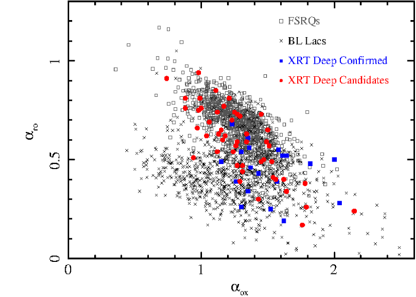
Figure 1: The $\alpha_{\rm ro}$ - $\alpha_{\rm ox}$ distribution for candidates blazar in our sample (large purple stars and blue crosses) superimposed to the one based on the blazars included in the BZCAT5 catalog (small circles).

After removing the sources that either were clearly not blazars or had bad counterparts, the sample includes 62 good X-ray radio associations with an optical counterpart. We present these sources in Table 1, where column 1: name from Swift Serendipitous Survey in deep XRT GRB Fields catalog; column 2: Right Ascension (J2000) from SDSS; column 3: Declination (J2000) from SDSS; column 4: Radio flux at 1.4GHz; column 5: X-ray flux in the 0.5-2 KeV band; column 6: SDSS redshift (when measured); column 7: logarithm in base 10 of the synchrotron peak $\nu_{peak}$ ; column 8: logarithm in base 10 of $\nu F_{\nu}$; column 9: the LR value; column 10: classification.

We used a third order polynomial fit to calculate the synchrotron peak $\nu_{peak}$ and we found 1 HSP blazars, although it has a high uncertainty in the determination of $\nu_{peak}$ due to lack of data. We used the SSDC SED tool to fit the data, which, unfortunately, at present does not estimate the $\nu_{peak}$ error.

Of the 62 sources, 19 were found to be blazars based on their available optical spectra, and, among these, 8 are BL Lacs and 11 FSRQs. For the classification in Table 1 we followed the one used in BZCAT5, that is BZB for BL Lac objects, BZQ for FSRQs in case of confirmed blazars, and BZG when the galaxy is clearly dominating the optical emission with respect to the nucleus. We classify the object as Candidate in the remaining cases.

If we consider the confirmed blazars only, the fraction of HSPs is $\sim 5\%$ $(i.e.1/19)$. The completion of the identification of the candidates is necessary to proper estimate the fraction of HPSs in the overall sample. However, we would like to note that the fraction of HSPs in an X-ray selected sample, which also has a radio cut such as ours, depends very much on the X-ray flux. In fact, most of HPSs are BL Lac objects; then, as shown in Fig. 5, simulations predict that at low X-ray fluxes the ratio between FSRQs and BL Lacs changes, with FSRQs becoming the main blazar subclass, therefore implying a possible change also in the percentage of HSPs in a given sample. Future studies will analyse this in more detail.

The distribution of the slopes between radio-optical and optical-X-ray for our sample superimposed to the one in the BZCAT5 catalog is shown in Figure 1, where $\alpha_{\nu_{1}\nu_{2}}$ is defined as:

$$\alpha_{\nu_{1}\nu_{2}}=-\frac{\log(f_{1}/f_{2})}{\log(\nu_{1}/\nu_{2})}.$$ (6)

We converted our radio flux from $1.4$ GHz to 5GHz using a power law with index $-0.25$; the X-ray frequency is chosen at 1 KeV. Our sample falls well on the region populated by the BZCAT5 blazars.

We noticed that in Fig. 1 the area defined by $\alpha_{\rm ox}$ $>1.3$ and $\alpha_{\rm ro}$ $<0.6$ is more crowded with candidates. Two reasons can account for the presence of this tail in the distribution of our sources at the right-lower bottom on the plane $\alpha_{\rm ox}$ -$\alpha_{\rm ro}$ , namely: i) the area is defined by the intersection of the two branches of LPSs and HSPs, therefore it is populated mainly by sources having $\nu_{peak}$ at intermediate frequencies, therefore the density of sources in this region of the plot simply reflects the statistical occurrence of ISPs; ii) possible contamination of thermal radiation for weak X-ray sources that would affect their $\alpha_{\rm ro}$ and $\alpha_{\rm ox}$ indices. More specifically, in the case of BL Lacs, the contribution from host galaxy light in the optical will cause the $\alpha_{\rm ro}$ to decrease to lower values, and in the meantime $\alpha_{\rm ox}$ to move to greater values, whereas in the case of FSRQs, the contribution of the Big Blue Bump in the optical will also make $\alpha_{\rm ro}$ to decrease, while we infer that at the same time $\alpha_{\rm ox}$ will probably remain almost constant, as the observed relation between the X-ray thermal radiation in the corona of quasars, and the optical/UV emission from the disk can be described by the a well-established anti-correlation between the $\alpha_{\rm ox}$ and the UV luminosity (see e.g. Vagnetti et al., 2010; Lusso & Risaliti, 2016; Chiaraluce et al., 2018). However, we underline that these heuristic arguments are just a starting point for a proper discussion, and they could be investigated properly only by dedicated simulations of X-ray selected samples at low X-ray fluxes, and confirmed later with future studies.

We calculated the LogN-LogS in the radio band at 5GHz and in the X-ray band using our final sample, reaching very deep fluxes. We will present these new LogN-LogS in the following sections, moving from the lowest (radio) to the highest energy (X-ray).

4 The radio LogN-LogS

The LogN-LogS of a population of sources in a given energy band can be used to estimate the emission in other parts of the electromagnetic spectrum, once the flux ratio in the two bands, or even better, the overall energy distribution, is known.

We used our new blazar sample to estimate the radio LogN-LogS of blazars with fluxes down to 10 mJy.

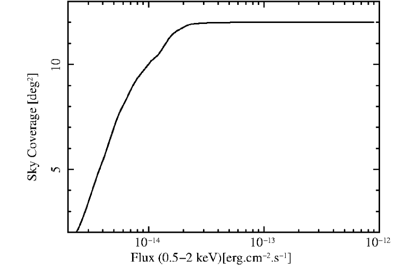
Figure 2: Sky coverage of the survey in terms of the X-ray flux for our sample of faint blazars.

We show in Fig. 3 our results together with calculations from previous surveys (see Appendix A for details). Since the radio surveys considered in this context have been carried out at different observing frequencies (1.4, 2.7 and 5 GHz), we converted all flux densities to a common band. We selected 5 GHz as the reference frequency and we apply flux conversions assuming as above a spectral slope $\alpha_{r}=0.25$ ($f_{\nu}\sim\nu^{-\alpha_{r}}$) which is approximately equal to the average value in all the considered samples.

The completeness limit of the NVSS is $\sim 2.5$mJy whereas the detection limit is $\sim 1$mJy over most of the FIRST survey. The sensitivity of SUMSS is similar to that of the NVSS. This implies a quite flat radio sky coverage over our GRB fields with a radio cut at $\sim 2.5$mJy. As consequence, we take into account the X-ray sky coverage to calculate the radio logN-logS, as we are not sampling the X-ray sky homogeneously over the different fields.

We used the Swift sky coverage (see Figure 2) for the GRB fields covered by SDSS photometry (S. Puccetti, private communication) in order to calculate the counts in the final sample, plotted in Fig 3 as red filled circles (color figure available online only). We considered that the sky coverage in Fig. 2 points out that faint objects with flux around 10^-14 erg cm^-2 s^-1 could be detected only in $\sim$ 8 square degrees, whereas objects one order of magnitude brighter (i.e. flux $\sim$ 10^-13 erg cm^-2 s^-1) could be detected in $\sim$ 10 square degrees. Taking this into account, we followed the method used for the One Jansky ASDC-RASS-NVSS blazar sample (Giommi et al., 2006) to calculate the radio counts for our final sample at 1.4 GHz. In particular, for each source we used the radio flux to count the object in the corresponding bin of radio flux density, and the X-ray flux to estimate the area covered by the survey from the X-ray sky coverage. Then, we converted the flux densities to 5 GHz to obtain the final logN-logS, assuming a spectral slope of 0.25 as we did for the other surveys. Given the small area of the Swift survey ($\approx 12$ square degrees), and the low space density of blazars, our sample can probe only the faint tail of the radio LogN-LogS.

Considering the overall derived counts N($>$S) from the different surveys, they are consistent with a broken powerlaw described as $S^{-1.66}$ for fluxes $S>10~{}mJy$, with a break at $S\approx 10~{}mJy$. We have to note that the slope below the break cannot be estimated accurately as the optical spectra available allows us to calculate only lower limits to the density of blazars: however, we underline that for fluxes $S<10~{}mJy$ a slope flattening is required also in order to avoid that the predicted blazar space density exceeds the observed total density of radio sources at a few mJy (e.g. NVSS, FIRST) which we plot in Fig. 3 as upper limits. We chose to model the slope below the break as $S^{-0.9}$, since $-0.9$ is the average slope of the logN-logS of radio quiet AGN in the two flux decades below the break (Rosati et al., 2002; Moretti et al., 2003) and we found that it is consistent with the available constraints. Our results are consistent with previous work on this topic (Giommi et al., 2006), that reported a good fit to previously known data as $S^{-1.62}$ for fluxes $S>15~{}mJy$ and pointed out for the presence of a break below 15 mJy.

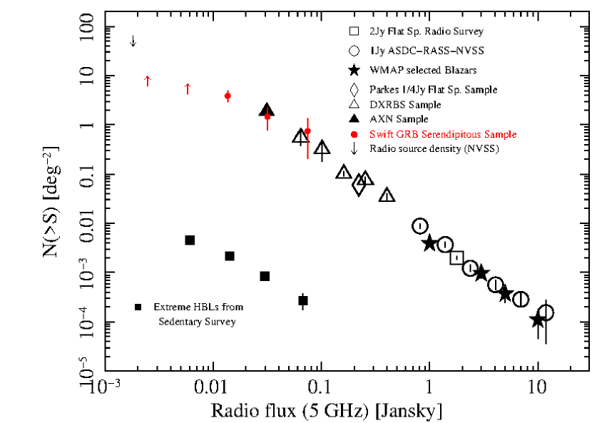
Figure 3: The radio (5 GHz) LogN-LogS of candidate blazars that extends to fluxes down to 10 mJy the blazar radio LogN-LogS built combining several radio and multi-frequency surveys. We show counts from each survey using different symbols (see text for details). The filled squares in the lower left part represent for comparison the radio LogN-LogS of extreme HBL BL Lacs from the Sedentary Survey.

However, we must consider the possibility that our sample is still contaminated within a certain amount by other non-thermal AGN characterized by steep radio spectrum, such as radio galaxies and steep spectrum quasars, with respect to blazars that show flat radio spectral slopes. Further multifrequency data, especially in the radio band and optical spectra, are needed to get conclusive classifications for our candidates.

Nonetheless, we would like to underline that at the lowest fluxes we could also start missing blazar identifications not only for the X-ray sky coverage but also given the radio cut and our request to have an optical counterpart in SDSS data. In fact, for example, it has been estimated that in case of SDSS-DR10, objects from the FIRST survey have $\sim 30\%$ of optical identifications at SDSS magnitude limit ($m_{V}\sim 23$). Therefore, we are using lower limits on the density of blazars for the logN-logS points at the lowest fluxes in Fig. 3, just in order to make more evident to the reader that the possibility of missing objects at these fluxes.

5 The X-ray LogN-LogS

The X-ray Log N-Log S for our sample of candidate blazars is shown in Figure 4. It reaches very faint fluxes (below $10^{-14}$ erg cm^-2s^-1 in the 0.5-2.0 keV band) and it is therefore by far the deepest to date. We calculated the upper limits in Fig. 4 assuming that all our candidates are blazars, whereas filled points represent actual number density for the confirmed blazars in the sample, i.e. confirmed on the basis of their optical spectra.

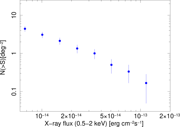
Figure 4: Total number density of the sources in our sample versus their X-ray fluxes.

It is useful to compare the LogN-LogS of our sample with previously published logN-logS of blazars. One of the more recent estimations was done by Giommi & Padovani (2015), who used a Monte Carlo simulated X-ray flux limited catalog to estimate the number counts of different types of faint blazars, showing that it agrees very well with previous estimates at bright fluxes. To compare our results with this one, it is necessary to rescale fluxes in our soft band (0.5-2 keV) to match the one used in the paper (0.3-3.5 keV) mentioned above. Assuming an energy distribution with a power law index of 0.9, the correction factor is 1.87.

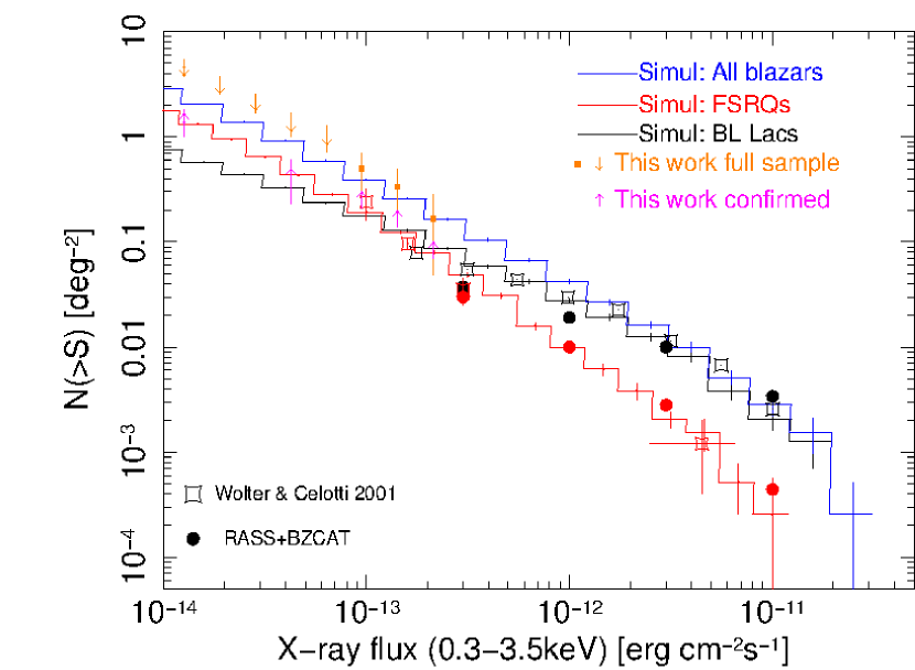
Figure 5: X-ray LogN-LogS of our final Swift sample compared to the one of Giommi & Padovani (2015). Orange arrows and filled squares correspond to the full sample (candidates and confirmed blazars), purple arrows are the spectroscopically confirmed blazars only. While our full sample overestimates the number of sources for faint fluxes ($\lesssim 10^{-13}$ erg cm^-2s^-1), the number of confirmed blazars is still below the simulated counts. See text for details.

As we can see from Figure 5, we are in good agreement at high fluxes, whereas our upper limits (orange downward arrows in the color figure available only online) estimated assuming that all our candidates are blazars overestimate the counts of Giommi & Padovani (2015) at the faint end. This is very likely due to the fact that not all of our sources will turn out to be confirmed as blazars. On the other hand, if we build the LogN-LogS using only for the confirmed blazars (19 out of the 62, shown as purple arrows in the color figure available only online), we see that we are below the number predicted by the simulations. Therefore, both our number counts and the simulations of Giommi & Padovani (2015) could be in agreement after the removal of the non-blazar sources of our sample.

With respect to Wolter & Celotti (2001), our sample can probe populations of sources 10 times weaker in the X-ray flux, thus allowing for a more detailed comparison between data and simulated counts. In particular, as shown in Figure 5, simulations of Giommi & Padovani (2015) predict the inversion of the population density of BL Lacs and FSRQs at lower fluxes. So far it was not possible to investigate this outcome from the simulations as the inversion was expected to happen at fluxes not reached by previous available samples. Therefore, we highlight that the complete classification of our candidates by means of optical spectra will be crucial to explore the properties of blazars at the really faint end of their Log N-Log S.

Given the small area covered by Swift, however, our sample can be used to study only populations below $10^{-13}$ erg cm^-2s^-1. On the contrary, data from the RASS-BZCAT sample (see for details Giommi & Padovani, 2015) cover a sufficiently large area of the sky to investigate the numbers of FSRQs at high fluxes ($>10^{-12}$ erg cm^-2s^-1), and it can be used to complement information from our sample.

Furthermore, future studies of X-ray selected samples of faint blazars with eROSITA (Merloni et al., 2012) will shed more light on the blazar population at low X-ray fluxes.

Table 1: Catalog of faint blazars and blazar candidates.

NAME	SDSS RA	SDSS DEC	Flux1.4GHz	Flux0.5-2keV	z	Log($\nu_{p})$	Log($\nu F_{\nu}$)	LR	Class
	(J2000, deg)	(J2000, deg)	(mJy)	(units of $10^{-14}$)
				(erg cm-2s-1)
SWIFTFTJ001252.7$+$3241.6	3.22250	32.69389	8.20	3.44	-	12.5∗	-12.5∗	0.012	Candidate
SWIFTFTJ005503.5$+$1408.0	13.76417	14.13500	99.9	4.10	1.666	13.1	-12.5	1.852	BZQ
SWIFTFTJ005514.7$+$1407.4	13.81083	14.12417	19.9	2.13	-	13.5	-12.7	1.872	Candidate
SWIFTFTJ012320.3$+$3812.9	20.83458	38.21583	6.70	0.345	-	12.1∗	-12.3∗	0.980	Candidate
SWIFTFTJ020726.5$+$0022.5	31.86042	0.37611	61.8	0.671	-	∗	∗	0.594	Candidate
SWIFTFTJ021305.6$-$0219.4	33.27333	-2.32333	32.2	1.94	1.670	12.4∗	-12.6∗	1.723	BZQ
SWIFTFTJ021307.9$-$0212.3	33.28416	-2.20528	11.4	0.935	-	∗	∗	0.198	Candidate
SWIFTFTJ024446.7$-$0210.0	41.19417	-2.16806	1.60	2.15	2.012	12.5∗	-12.6∗	1.373	BZQ
SWIFTFTJ033630.2$+$1723.2	54.12542	17.38778	19.9	2.66	-	13.3∗	-13.1∗	0.546	Candidate
SWIFTFTJ054613.3$+$6410.5	86.55625	64.17611	12.6	0.490	-	∗	∗	1.715	Candidate
SWIFTFTJ062257.9$-$0109.4	95.74084	-1.15611	241.0	3.45	-	12.9	-12.7	0.074	Candidate
SWIFTFTJ075144.8$+$3107.9	117.93667	31.13222	24.2	0.362	-	13.0∗	-12.8∗	1.768	Candidate
SWIFTFTJ084803.7$+$1338.8	132.01543	13.64750	1.90	0.367	-	12.8∗	-12.7∗	0.911	Candidate
SWIFTFTJ084842.8$+$1336.3	132.17917	13.60639	7.60	1.43	-	12.8∗	-12.5∗	0.355	Candidate
SWIFTFTJ085542.7$+$1103.2	133.92792	11.05389	14.8	9.19	0.300	15.1∗1	-12.5∗	1.727	BZG
SWIFTFTJ090602.1$+$3512.1	136.50792	35.20417	3.20	0.423	-	12.8∗	-12.3∗	0.000	Candidate
SWIFTFTJ090936.0$+$4547.5	137.39917	45.79306	24.7	0.547	0.321	13.8∗	-12.8	1.126	BZG
SWIFTFTJ090954.4$+$4544.3	137.47708	45.73667	57.8	4.12	-	12.9	-13.0	0.003	Candidate
SWIFTFTJ091036.3$+$4537.2	137.65042	45.62083	2.70	0.716	-	13.6∗	-13.0∗	0.442	Candidate
SWIFTFTJ093045.1$+$1659.4	142.68918	16.99139	72.5	0.280	0.177	13.5∗	-12.5∗	1.062	BZG
SWIFTFTJ093750.9$+$1536.5	144.46251	15.60972	4.60	0.649	-	∗	∗	1.846	Candidate
SWIFTFTJ101433.3$+$4306.0	153.63916	43.10194	4.90	1.52	1.684	∗	∗	0.592	BZQ
SWIFTFTJ101609.4$+$4336.2	154.03917	43.60278	3.70	11.7	0.587	13.4∗	-12.6∗	0.762	BZQ
SWIFTFTJ101700.5$+$4328.3	154.25249	43.47195	5.90	0.757	-	12.5∗	-12.7∗	1.458	Candidate
SWIFTFTJ101727.4$+$4329.0	154.36417	43.48444	197.1	5.12	1.175	12.7	-12.5	1.745	BZQ
SWIFTFTJ110035.7$+$5148.2	165.14958	51.80333	4.20	1.47	-	14.0∗	-13.0∗	0.483	Candidate
SWIFTFTJ114449.6$+$5953.3	176.20667	59.88861	6.00	0.913	-	∗	∗	1.660	Candidate
SWIFTFTJ115036.9$+$5707.6	177.65500	57.12806	17.2	0.733	0.117	14.3∗	-13.6∗	0.150	BZG
SWIFTFTJ120512.5$+$4007.0	181.30125	40.11583	6.00	0.431	2.434	13.6∗	-13.1∗	0.455	BZQ
SWIFTFTJ121012.4$+$3959.0	182.55292	39.98417	4.50	0.512	0.562	∗	∗	1.297	BZG
SWIFTFTJ123405.8$+$2102.4	188.52415	21.04028	1.20	1.29	-	13.1∗	-13.0∗	1.860	Candidate
SWIFTFTJ130358.6$+$4110.1	195.99542	41.16972	1.90	0.604	1.212	∗	∗	0.081	BZQ
SWIFTFTJ131215.9$+$6200.9	198.06792	62.01694	16.3	2.82	-	13.6∗	-13.0∗	0.137	Candidate
SWIFTFTJ132332.3$+$4043.5	200.88834	40.72722	28.6	3.00	-	13.3∗	-13.2∗	0.008	Candidate
SWIFTFTJ132928.6$+$4230.7	202.37000	42.51361	30.5	0.942	1.597	13.0∗	-12.9∗	0.940	BZQ
SWIFTFTJ133128.5$+$4209.7	202.86958	42.16195	1.30	1.17	0.939	12.8	-12.4	0.710	BZQ
SWIFTFTJ133201.5$+$3458.9	203.00667	34.98361	0.80	0.0997	-	13.6	-13.2	1.000	Candidate
SWIFTFTJ134931.4$+$0732.7	207.38167	7.54528	5.00	1.18	-	13.9∗	-12.6∗	0.871	Candidate
SWIFTFTJ141144.6$+$1655.2	212.93875	16.92194	1.60	2.07	0.615	∗	∗	0.00	BZB
SWIFTFTJ143133.6$+$3628.0	217.88792	36.46611	4.70	0.183	-	12.7∗	-13.0∗	0.035	Candidate
SWIFTFTJ143733.7$+$2743.3	219.39041	27.72278	15.7	0.208	0.310	14.0∗	-12.8∗	1.709	BZG
SWIFTFTJ144021.7$-$0004.6	220.09041	-0.07722	16.7	0.440	-	13.5∗	-13.4∗	0.999	Candidate
SWIFTFTJ144050.1$+$3333.8	220.20876	33.56389	7.00	4.20	1.777	12.6∗	-12.2∗	1.729	BZQ
SWIFTFTJ144615.4$+$5437.0	221.56459	54.61861	1.00	2.37	-	14.2∗	-13.4∗	1.055	Candidate
SWIFTFTJ151338.1$+$3048.2	228.40958	30.80333	3.40	4.61	-	14.0∗	-12.6∗	0.279	Candidate
SWIFTFTJ151526.3$+$4424.0	228.85918	44.40250	15.8	0.647	-	13.2∗	-12.9∗	0.109	Candidate
SWIFTFTJ153133.2$+$6327.8	232.88792	63.46305	64.0	0.515	-	∗	∗	1.453	Candidate
SWIFTFTJ153143.3$+$0020.3	232.93126	0.33639	37.3	0.911	-	13.1∗	-12.9∗	0.003	Candidate
SWIFTFTJ154059.3$+$6205.0	235.24791	62.08278	1.40	1.20	-	13.3	-12.1	1.139	Candidate
SWIFTFTJ155127.7$+$4447.4	237.86667	44.78944	6.30	0.663	-	12.0∗	-12.9∗	0.527	Candidate
SWIFTFTJ165845.5$+$1220.4	254.68916	12.34167	77.5	1.81	-	13.2	-12.9	1.765	Candidate
SWIFTFTJ183230.6$+$4230.2	278.12668	42.50389	25.0	14.0	-	13.5	-12.4	0.377	Candidate
SWIFTFTJ213156.7$+$0246.0	322.98584	2.76861	15.4	0.415	0.387	∗	∗	1.850	BZG
SWIFTFTJ215415.6$+$1652.6	328.56543	16.87611	17.1	5.57	-	12.8∗	-12.8∗	0.987	Candidate
SWIFTFTJ215436.0$+$1653.2	328.65082	16.88667	5.20	0.448	-	13.8∗	-13.1∗	0.230	Candidate
SWIFTFTJ220849.1$+$0652.3	332.20416	6.87278	229.4	7.73	-	14.5	-12.3	1.048	Candidate
SWIFTFTJ222507.4$-$0223.4	336.28168	-2.39111	39.1	2.00	-	∗	∗	1.079	Candidate
SWIFTFTJ224220.2$+$2346.8	340.58417	23.78167	25.2	0.356	-	12.7∗	-12.9∗	1.761	Candidate
SWIFTFTJ230410.9$+$0357.4	346.04459	3.95778	9.40	1.69	-	13.6∗	-12.∗	1.625	Candidate
SWIFTFTJ232236.8$+$0538.9	350.65335	5.64889	4.70	1.03	-	13.8∗	-12.9∗	1.997	Candidate
SWIFTFTJ232311.1$+$0543.1	350.79541	5.71917	9.10	0.471	-	12.4∗	-12.6∗	0.323	Candidate
SWIFTFTJ234732.3$+$0016.9	356.88541	0.28361	1.20	0.666	-	13.0	-12.9	0.057	Candidate
Notes: 1 HSP
∗ Uncertain value

6 Conclusions

By using faint sources serendipitously detected in Swift GRB fields and cross-matching them with radio surveys, we built a flux-limited catalog of blazar candidates down to very faint X-ray fluxes, a region that was lacking coverage in previous blazar research. Restricting ourselves to the area covered by the SDSS, we managed to obtain magnitudes and spectra (when available) for several of our sources. We used this sample of blazar candidates to calculate the radio LogN-LogS of Blazars with fluxes approximately down to 10 mJy. We were also able to estimate the soft X-ray LogN-LogS of blazars down to fluxes at least one order of magnitude fainter than previous works. A comparison with the expectations from Monte Carlo simulations of X-ray surveys indicates that our catalog is somewhat contaminated by sources other than blazars. However, the number counts of the spectroscopically confirmed sources still falls below the expected densities. Therefore, a complete optical follow-up is necessary to refine the sample. Moreover, high frequency radio observations are needed to measure the spectral slope for the candidates which have radio measurements at a single frequency. In fact, high frequency data can better evaluate the nuclear spectra, as the slopes at lower frequencies could be affected by the contribution from radio extended components in the jet. Useful data for this purpose could in principle be already present in the VLA archive as many radio observations are carried out at the VLA once a GRB explodes in order to catch its radio afterglow. Otherwise, the new JVLA (Chandler & Butler, 2014; Perley et al., 2009) and the upgraded ATCA (Wong & Melatos, 2002) are both promising to explore the spectral slope of the candidates as both these arrays have wider spectral radio bands. In particular, useful data will probably come from the on-going VLA Sky Survey (VLASS; Lacy et al. in preparation).

Completing the spectroscopical identification is crucial also because it will allow us to study the two main sub-populations of blazars, in particular regarding the inversion of their relative number density at low fluxes. We stress that to date the cosmological evolution properties of blazars have been studied on a few samples with a sufficiently large size. So far, it has been established that FSRQ evolve positively, both in radio and X-ray selected samples, as showed by Wolter & Celotti (2001), with the first X-ray selected sample for FSRQs. Results from literature indicate a higher evolution for X-ray selected quasars, although consistent at the $2\sigma$ level (Wolter & Celotti, 2001). Less clear is the trend among the BL Lac objects; however there seems to be a difference between the two classes: LSP BL Lacs show a slight positive evolution, consistent with no evolution at the $2\sigma$ level (Stickel et al., 1991), quite similar to radio selected FSRQs. HPS BL Lacs instead, show a negative evolution, more or less at the same $\sigma$ level, (Rector et al., 2000), indicating that the X-ray bright objects are less luminous or less numerous at high redshifts.

It has been shown that FSRQs evolve positively, whereas BL Lacs show no strong evolution also in the 15-55 KeV band, using an X-ray selected sample with data from the BAT instrument onboard Swift (Ajello et al., 2009). Instead, BL Lacs show positive evolution in case of $\gamma$-ray selected sample, with the relevant exception of low-luminosity HSP BL Lacs, which exhibit strong negative evolution (Ajello et al., 2014). Recently, Caccianiga et al. (2019) studied a sample of 26 high-redshift ($z>4$) radio-selected FSRQs, and found results in agreement with the predictions from the luminosity function derived on a radio-selected sample of FSRQs at lower redshifts (Mao et al., 2017), i.e. consistent with a peak in the space densities of FSRQs at $z\sim 2$, similar to what is found for radio-quiet QSOs. However, these findings on FSRQs are in tension with the results from the BAT X-ray selected sample, which on the contrary found a peak at $z\sim 4$ (Ajello et al., 2009). To date, there is no clear explanation of this difference, and further investigation is needed, especially to constrain the evolution of sources at lower luminosity.

Therefore, completing the optical identifications for our candidates will be important in this context as we will be able to investigate blazar cosmological properties down to really faint fluxes, 10 times weaker than probed by previous works.

We have to note however - as also stated in Mignani (2009) - that the currently available public optical surveys do not provide sufficient data and spectra to support a systematic X-ray source identification work. Our work was carried out using object lists matching SDSS optical sources. Unfortunately there is not an analogous of the SDSS photometric survey in the southern sky: in fact, the USNO-B1 (Monet et al., 2003) catalog is too shallow to search for optical counterparts for the Swift radio-X associations lying in the southern sky. USNO-B1 limiting magnitude is $R\approx 20$, whereas SDSS limiting magnitude is deeper, $r^{\prime}\sim 22$. This represents a severe limitation since the deepest flux limits reached by the Swift survey requires of course similarly deeper optical catalogs to homogeneously sample the $\alpha_{\rm ox}$ -$\alpha_{\rm ro}$ parameter space. Surely, on-going and next generation surveys in the southern emisphere, such as VISTA (Worswick et al., 2000), Pan-STARSS (Kaiser et al., 2010) and LSST (Tyson et al., 2012), will provide useful data for optical identifications of faint high energy sources.

Appendix A Previous Surveys for the radio LogN-LogS

We give in the following some details regarding the other blazar surveys shown in Fig. 3 in order of decreasing radio flux limit:

1. The 2Jy Flat Spectrum Radio Survey is a sample of 60 confirmed blazars (di Serego-Alighieri et al., 1994; Urry & Padovani, 1995) included in the 2Jy 2.7 GHz sample (Wall & Peacock, 1985), based on a complete radio flux limited survey of flat spectrum ($\alpha_{r}<0.5$) sources covering the entire sky with the exclusion of the Galactic plane ($|b|>10$). The corresponding blazar space density is $0.002~{}deg^{-2}$ and this value is plotted as open squares in Fig. 3.

2. The 1Jy ASDC-RASS-NVSS blazar sample (Giommi et al., 2002) is a radio flux limited ($f_{r}<1Jy$ at 1.4 GHz) sample built via a cross-correlation between the ROSAT All Sky Survey (RASS) catalog of X-ray sources (Voges et al., 1999) and the subsample of NVSS sources with flux densities larger than 1 Jy. The blazars within the sample are 160 over 226 total sources. This sample was used to estimate the blazar space density above 1 Jy taking into account the RASS sky coverage, the counts were converted to 5 GHz and are plotted as open circles in Fig 3.

3. The WMAP selected Blazars sample (see Giommi et al., 2009) comprises $\sim 87\%$ of WMAP foreground source detections. The counts are show in Fig. 3 as filled stars and are in good agreement with other radio survey at cm wavelength, except for the point at 1 Jy, which is most likely underestimated as the WMAP catalog is incompleted at this flux limit (Bennett et al., 2003).

4. The Parkers 1/4Jy Flat Spectrum Sample (Wall et al., 2005) is a 100% identified radio flux limited survey at 2.7 GHz. The blazar space density inferred by this survey is 0.06 objects per square degree and is show in Fig. 3 as open diamonds.

5. The DXRBS (Deep X-ray Radio Blazar Survey) Sample is a radio flux limited sample based on a double selection technique at radio and X-ray frequencies and uses optical data to refine the sample (see e.g. Perlman et al., 1998; Landt et al., 2001; Padovani et al., 2007). The blazar space density from Padovani et al. (2007) is plotted in Fig. 3 as open triangles.

6. The AXN (ASDC-XMM-Newton-NVSS) Sample (Giommi et al., 2006) pushes the DXRBS selection technique to fluxes down 50 mJy. The counts at 50 mJy are shown in Fig. 3 as a black filled circle, whereas the estimated lower limits at fainter fluxes are shown as black arrows.

7. The counts from the Extreme HBL from the Sedentary Survey (see e.g. Giommi et al., 1999; Giommi et al., 2005; Piranomonte et al., 2007) are shown in Fig. 3 as filled squares. This sample is a deep ($f_{r}\geq 3.5~{}mJy$ at 1.4 GHz), 100% identified radio flux limited sample of 150 extreme HBL objects characterized by $f_{\rm x}/f_{\rm r}$  ratio higher than $3\times 10^{-10}$ erg cm^-2s^-1Jy^-1 . This survey does not have a direct impact on the full blazar LogN-LogS shown in Fig. 3 as these sources represent only a tiny fraction of the overall blazar population. However, their very high $f_{\rm x}/f_{\rm r}$  makes them potentially significant contributors to the Cosmic background in the high energy bands, such as X-ray, $\gamma$-ray and TeV.

Appendix B Additional sources

Some objects were not included in the final Swift deep GRB pointings catalog as they were just above the probability threshold fixed for detection. Despite that, we found that seven of these sources have good radio and optical counterparts. We list them in Table 2. Also among them there is a HSP blazar, however also in this case there is a high uncertainty in the determination of $\nu_{peak}$ due to lack of data. However, we underline here that we did not use these objects in the calculation of the radio and X-ray LogN-LogS, presented in the Sections 4 and 5.

Table 2: Sources above the probability threshold of the Swift Serendipitous Survey in deep XRT GRB Fields catalog.

RA (J2000)	DEC (J2000)	Flux1.4GHz	Flux0.5-2keV	Log($\nu_{p})$	Log($\nu F_{\nu}$)	LR
(deg)	(deg)	(mJy)	($10^{-14}$erg cm-2s-1)
02 19 33.5	68 44 41.7	4.00	1.02	15.4∗1	-11.9	1.165
03 36 32.7	17 16 56.1	54.8	1.36	14.1∗	-12.6	1.717
09 30 06.7	16 54 31.4	2.10	0.175	12.6∗	-12.6	1.493
11 50 41.0	57 18 19.1	2.90	0.188	14.4	-12.5	0.923
14 36 45.9	27 42 31.2	7.50	0.173	14.8∗	-12.2	1.545
16 59 02.0	12 27 55.7	3.00	1.64	14.2	-13.0	0.872
21 55 11.3	16 50 58.3	6.40	1.24	14.8	-12.6	0.040
Notes: 1 HSP
∗ Uncertain value

References

- Abdo et al. (2010) Abdo A. A., et al., 2010, ApJ, 716, 30
- Abolfathi et al. (2018) Abolfathi B., et al., 2018, ApJS, 235, 42
- Ackermann et al. (2017) Ackermann M., et al., 2017, ApJ, 837, L5
- Ajello et al. (2009) Ajello M., et al., 2009, ApJ, 699, 603
- Ajello et al. (2014) Ajello M., et al., 2014, ApJ, 780, 73
- Arsioli et al. (2015) Arsioli B., Fraga B., Giommi P., Padovani P., Marrese P. M., 2015, A&A, 579, A34
- Becker et al. (1995) Becker R. H., White R. L., Helfand D. J., 1995, ApJ, 450, 559
- Bennett et al. (2003) Bennett C. L., et al., 2003, ApJS, 148, 97
- Blandford & Rees (1978) Blandford R. D., Rees M. J., 1978, Phys. Scr., 17, 265
- Boller et al. (2016) Boller T., Freyberg M. J., Trümper J., Haberl F., Voges W., Nandra K., 2016, A&A, 588, A103
- Caccianiga et al. (2019) Caccianiga A., et al., 2019, MNRAS, 484, 204
- Chandler & Butler (2014) Chandler C. J., Butler B. J., 2014, in Observatory Operations: Strategies, Processes, and Systems V. p. 914917, doi:10.1117/12.2057106
- Chiaraluce et al. (2018) Chiaraluce E., Vagnetti F., Tombesi F., Paolillo M., 2018, A&A, 619, A95
- Condon et al. (1998) Condon J. J., Cotton W. D., Greisen E. W., Yin Q. F., Perley R. A., Taylor G. B., Broderick J. J., 1998, AJ, 115, 1693
- D’Abrusco et al. (2014) D’Abrusco R., Massaro F., Paggi A., Smith H. A., Masetti N., Landoni M., Tosti G., 2014, ApJS, 215, 14
- Gehrels et al. (2004) Gehrels N., et al., 2004, ApJ, 611, 1005
- Gioia et al. (1990) Gioia I. M., Maccacaro T., Schild R. E., Wolter A., Stocke J. T., Morris S. L., Henry J. P., 1990, ApJS, 72, 567
- Giommi & Padovani (2015) Giommi P., Padovani P., 2015, MNRAS, 450, 2404
- Giommi et al. (1999) Giommi P., Menna M. T., Padovani P., 1999, MNRAS, 310, 465
- Giommi et al. (2002) Giommi P., Perri M., Piranomonte S., Padovani P., 2002, in Giommi P., Massaro E., Palumbo G., eds, Blazar Astrophysics with BeppoSAX and Other Observatories. p. 123
- Giommi et al. (2005) Giommi P., Piranomonte S., Perri M., Padovani P., 2005, A&A, 434, 385
- Giommi et al. (2006) Giommi P., Colafrancesco S., Cavazzuti E., Perri M., Pittori C., 2006, A&A, 445, 843
- Giommi et al. (2009) Giommi P., Colafrancesco S., Padovani P., Gasparrini D., Cavazzuti E., Cutini S., 2009, A&A, 508, 107
- Kaiser et al. (2010) Kaiser N., et al., 2010, in Society of Photo-Optical Instrumentation Engineers (SPIE) Conference Series. , doi:10.1117/12.859188
- Landt et al. (2001) Landt H., Padovani P., Perlman E. S., Giommi P., Bignall H., Tzioumis A., 2001, MNRAS, 323, 757
- Lusso & Risaliti (2016) Lusso E., Risaliti G., 2016, ApJ, 819, 154
- Madrid & Macchetto (2009) Madrid J. P., Macchetto D., 2009, in Bulletin of the American Astronomical Society. pp 913–914 (arXiv:0901.4552)
- Mao et al. (2017) Mao P., Urry C. M., Marchesini E., Landoni M., Massaro F., Ajello M., 2017, ApJ, 842, 87
- Merloni et al. (2012) Merloni A., et al., 2012, arXiv e-prints,
- Mignani (2009) Mignani R. P., 2009, preprint, (arXiv:0902.0634)
- Monet et al. (2003) Monet D. G., et al., 2003, AJ, 125, 984
- Moretti et al. (2003) Moretti A., Campana S., Lazzati D., Tagliaferri G., 2003, ApJ, 588, 696
- Moretti et al. (2006) Moretti A., et al., 2006, A&A, 448, L9
- Padovani & Giommi (1995) Padovani P., Giommi P., 1995, ApJ, 444, 567
- Padovani et al. (2007) Padovani P., Giommi P., Landt H., Perlman E. S., 2007, ApJ, 662, 182
- Perley et al. (2009) Perley R., et al., 2009, IEEE Proceedings, 97, 1448
- Perlman et al. (1998) Perlman E. S., Padovani P., Giommi P., Sambruna R., Jones L. R., Tzioumis A., Reynolds J., 1998, AJ, 115, 1253
- Piranomonte et al. (2007) Piranomonte S., Perri M., Giommi P., Landt H., Padovani P., 2007, A&A, 470, 787
- Puccetti et al. (2011) Puccetti S., et al., 2011, A&A, 528, A122
- Rector et al. (2000) Rector T. A., Stocke J. T., Perlman E. S., Morris S. L., Gioia I. M., 2000, AJ, 120, 1626
- Richter (1975) Richter G. A., 1975, Astronomische Nachrichten, 296, 65
- Rosati et al. (2002) Rosati P., et al., 2002, ApJ, 566, 667
- Savaglio & Grothkopf (2013) Savaglio S., Grothkopf U., 2013, PASP, 125, 287
- Singh et al. (1995) Singh K. P., Barrett P., White N. E., Giommi P., Angelini L., 1995, ApJ, 455, 456
- Stickel et al. (1991) Stickel M., Fried J. W., Kühr H., Padovani P., Urry C. M., 1991, ApJ, 374, 431
- Sutherland & Saunders (1992) Sutherland W., Saunders W., 1992, MNRAS, 259, 413
- Turriziani et al. (2007) Turriziani S., Cavazzuti E., Giommi P., 2007, A&A, 472, 699
- Tyson et al. (2012) Tyson J. A., Ivezic Z., Strauss M., LSST Science Collaborations 2012, in American Astronomical Society Meeting Abstracts 219. p. 156.05
- Urry & Padovani (1995) Urry C. M., Padovani P., 1995, PASP, 107, 803
- Vagnetti et al. (2010) Vagnetti F., Turriziani S., Trevese D., Antonucci M., 2010, A&A, 519, A17
- Voges et al. (1999) Voges W., et al., 1999, A&A, 349, 389
- Voges et al. (2000) Voges W., et al., 2000, IAU Circ., 7432, 3
- Wall & Peacock (1985) Wall J. V., Peacock J. A., 1985, MNRAS, 216, 173
- Wall et al. (2005) Wall J. V., Jackson C. A., Shaver P. A., Hook I. M., Kellermann K. I., 2005, A&A, 434, 133
- Wolter & Celotti (2001) Wolter A., Celotti A., 2001, A&A, 371, 527
- Wong & Melatos (2002) Wong T., Melatos A., 2002, Publ. Astron. Soc. Australia, 19, 475
- Worswick et al. (2000) Worswick S. P., Atad-Ettedgui E., Casali M. M., Henry D. M., 2000, in P. Dierickx ed., Society of Photo-Optical Instrumentation Engineers (SPIE) Conference Series Vol. 4003, Society of Photo-Optical Instrumentation Engineers (SPIE) Conference Series. pp 373–380
- Żywucka et al. (2018) Żywucka N., Goyal A., Jamrozy M., Stawarz Ł., Ostrowski M., Kozłowski S., Udalski A., 2018, ApJ, 867, 131
- di Serego-Alighieri et al. (1994) di Serego-Alighieri S., Danziger I. J., Morganti R., Tadhunter C. N., 1994, MNRAS, 269, 998