New physics and tau $g-2$ using LHC heavy ion collisions

Abstract

The anomalous magnetic moment of the tau lepton $a_{\tau}=(g_{\tau}-2)/2$ strikingly evades measurement, but is highly sensitive to new physics such as compositeness or supersymmetry. We propose using ultraperipheral heavy ion collisions at the LHC to probe modified magnetic $\delta a_{\tau}$ and electric dipole moments $\delta d_{\tau}$. We introduce a suite of one electron/muon plus track(s) analyses, leveraging the exceptionally clean photon fusion $\gamma\gamma\to\tau\tau$ events to reconstruct both leptonic and hadronic tau decays sensitive to $\delta a_{\tau},\delta d_{\tau}$. Assuming 10% systematic uncertainties, the current 2 nb^-1 lead–lead dataset could already provide constraints of $-0.0080<a_{\tau}<0.0046$ at 68% CL. This surpasses 15 year old lepton collider precision by a factor of three while opening novel avenues to new physics.

I Introduction

Precision measurements of electromagnetic couplings are foundational tests of quantum electrodynamics (QED) and powerful probes of beyond the Standard Model (BSM) physics. The electron anomalous magnetic moment $a_{e}=\frac{1}{2}(g_{e}-2)$ is among the most precisely known quantities in nature Odom et al. (2006); Hanneke et al. (2011); Bouchendira et al. (2011); Aoyama et al. (2012a); Parker et al. (2018). The muon counterpart $a_{\mu}$ is measured to $10^{-7}$ precision Bennett et al. (2006) and reports a $3-4\sigma$ tension from SM predictions Aoyama et al. (2012b); Keshavarzi et al. (2018). This may indicate new physics Martin and Wells (2001); Czarnecki and Marciano (2001); Hagiwara et al. (2011); Ajaib et al. (2015), to be clarified at Fermilab Grange et al. (2015) and J–PARC Abe et al. (2019). Measuring $a_{\ell}$ generically tests lepton compositeness Silverman and Shaw (1983), while supersymmetry at energy scales $M_{\text{S}}$ induces radiative corrections $\delta a_{\ell}\sim m_{\ell}^{2}/M_{\text{S}}^{2}$ for leptons with mass $m_{\ell}$ Martin and Wells (2001). Thus the tau $\tau$ can be $m_{\tau}^{2}/m_{\mu}^{2}\sim 280$ times more sensitive to BSM physics than $a_{\mu}$.

However, $a_{\tau}$ continues to evade measurement because the short tau proper lifetime $\sim 10^{-13}$ s precludes use of spin precession methods Bennett et al. (2006). The most precise single-experiment measurement $a_{\tau}^{\text{exp}}$ is from DELPHI Abdallah et al. (2004); Tanabashi et al. (2018) at the Large Electron Positron Collider (LEP), but is remarkably an order of magnitude away from the theoretical central value $a_{\tau,\,\text{SM}}^{\text{pred}}$ predicted to $10^{-5}$ precision Eidelman and Passera (2007)

$$a_{\tau}^{\text{exp}}=-0.018\,(17),\quad a_{\tau,\,\text{SM}}^{\text{pred}}=0.001\,177\,21\,(5).$$ (1)

The poor constraints on $a_{\tau}$ present striking room for BSM physics, especially given other lepton sector tensions Dutta and Mimura (2019); Davoudiasl and Marciano (2018); Bauer et al. (2019); LHCb Collaboration (2015); Belle Collaboration (2019); Allanach et al. (2016); Di Chiara et al. (2017); Biswas and Shaw (2019), and motivate new experimental strategies.

This Letter proposes a suite of analyses to probe $a_{\tau}$ using heavy ion beams at the LHC. We leverage ultraperipheral collisions (UPC) where only the electromagnetic fields surrounding lead (Pb) ions interact. Tau pairs are produced from photon fusion $\text{PbPb}\to\text{Pb}(\gamma\gamma\to\tau\tau)\text{Pb}$, illustrated in Fig. 1, whose sensitivity to $a_{\tau}$ was suggested in 1991 del Aguila et al. (1991). We introduce the strategy crucial for experimental realization and importantly show that the currently recorded dataset could already surpass LEP precision. The LHC cross-section enjoys a $Z^{4}$ enhancement ($Z=82$ for Pb), with over one million $\gamma\gamma\to\tau\tau$ events produced to date. Existing proposals using lepton beams require future datasets (Belle-II) or proposed facilities (CLIC, LHeC) Koksal et al. (2018); Howard et al. (2018); Koksal (2018); Gutiérrez-Rodríguez et al. (2019); Fael et al. (2014); Eidelman et al. (2016); Chen and Wu (2018), while LHC studies focus on high luminosity proton beams Samuel and Li (1994); Hayreter and Valencia (2013); Atag and Billur (2010); Hayreter and Valencia (2013); Galon et al. (2016); Fomin et al. (2019); Fu et al. (2019). No LHC analysis of $\gamma\gamma\to\tau\tau$ exists as the taus have insufficient momentum for ATLAS/CMS to record or reconstruct.

Our proposal overcomes these obstructions in the clean UPC events ATLAS Collaboration (2018a), enabling selection of individual tracks from tau decays with no other detector activity akin to LEP Abdallah et al. (2004). We exploit recent advances in low momentum electron/muon identification ATLAS Collaboration (2018b); CMS Collaboration (2018a); ATLAS Collaboration (2019a) to suppress hadronic backgrounds. We then present a shape analysis sensitive to interfering SM and BSM amplitudes to enhance $a_{\tau}$ constraints. Our strategy also probes tau electric dipole moments $d_{\tau}$ induced by charge–parity (CP) violating new physics. This opens key new directions in the heavy ion program amid reviving interest in photon collisions Piotrzkowski (2001); Albrow et al. (2009); de Favereau de Jeneret et al. (2009) for light-by-light scattering d’Enterria and da Silveira (2013); ATLAS Collaboration (2017a); CMS Collaboration (2018b); ATLAS Collaboration (2019b), standard candle processes ATLAS Collaboration (2018c, 2016a); CMS Collaboration (2012, 2016); ATLAS Collaboration (2016b), and BSM dynamics Chapon et al. (2010); Fichet et al. (2014); Ellis et al. (2017); Knapen et al. (2017); Baldenegro et al. (2018); Ohnemus et al. (1994); Schul and Piotrzkowski (2008); Harland-Lang et al. (2012); Beresford and Liu (2018); Harland-Lang et al. (2019a); Bruce et al. (2018).

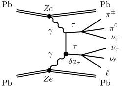
Figure 1: Pair production of tau leptons $\tau$ from ultraperipheral lead ion (Pb) collisions in two of the most common decay modes: $\pi^{\pm}\pi^{0}\nu_{\tau}$ and $\ell\nu_{\ell}\nu_{\tau}$. New physics can modify tau–photon couplings affecting the magnetic moment by $\delta a_{\tau}$.

II Effective theory & photon flux

The anomalous $\tau$ magnetic moment $a_{\tau}=(g_{\tau}-2)/2$ is defined by the spin–magnetic Hamiltonian $-\bm{\mu}_{\tau}\cdot\mathbf{B}=-(g_{\tau}e/2m_{\tau})\,\mathbf{S}\cdot\mathbf{B}$. In the Lagrangian formulation of QED, electromagnetic moments arise from the spinor tensor $\sigma^{\mu\nu}=\mathrm{i}[\gamma^{\mu},\gamma^{\nu}]/2$ structure of the fermion current interacting with the photon field strength $F_{\mu\nu}$

$$\mathcal{L}=\tfrac{1}{2}\bar{\tau}_{\text{L}}\sigma^{\mu\nu}\left(a_{\tau}\tfrac{e}{2m_{\tau}}-\mathrm{i}d_{\tau}\gamma_{5}\right)\tau_{\text{R}}F_{\mu\nu}.$$ (2)

Here, $\gamma^{5}$ satisfies the anticommutator $\{\gamma^{5},\gamma^{\mu}\}=0$, and $\tau_{\text{L,R}}$ are tau spinors with L,R denoting chirality.

To introduce BSM modifications of $a_{\tau}$ and $d_{\tau}$, we use SM effective field theory (SMEFT) Escribano and Masso (1993). This assumes the scale of BSM physics $\Lambda$ is much higher than the probe momentum transfers $q$ i.e., $q^{2}\ll\Lambda^{2}$. At scale $q$, two dimension-six operators in the Warsaw basis Grzadkowski et al. (2010) modify $a_{\tau}$ and $d_{\tau}$ at tree level, as discussed in Ref. Escribano and Masso (1993)

$$\mathcal{L}^{\prime}=\left(\bar{L}_{\tau}\sigma^{\mu\nu}\tau_{R}\right)H\left[\frac{C_{\tau B}}{\Lambda^{2}}B_{\mu\nu}+\frac{C_{\tau W}}{\Lambda^{2}}W_{\mu\nu}\right].$$ (3)

Here, $B_{\mu\nu}$ and $W_{\mu\nu}$ are the U(1)${}_{\text{Y}}$ and SU(2)${}_{\text{L}}$ field strengths, $H$ ($L_{\tau}$) is the Higgs (tau lepton) doublet, and $C_{i}$ are dimensionless, complex Wilson coefficients. We fix $C_{\tau W}=0$ to parameterize the two modified moments $(\delta a_{\tau},\delta d_{\tau})$ using two real parameters $(|C_{\tau B}|/\Lambda^{2},\varphi)$ Eidelman et al. (2016)

$$\delta a_{\tau} =\frac{2m_{\tau}}{e}\frac{|C_{\tau B}|}{M}\cos\varphi,\quad\delta d_{\tau}=\frac{|C_{\tau B}|}{M}\sin\varphi,$$ (4)

where $\varphi$ is the complex phase of $C_{\tau B}$, we define $M=\Lambda^{2}/(\sqrt{2}v\cos\theta_{W})$, $\theta_{W}$ is the electroweak Weinberg angle, and $v=246$ GeV.

In the SM, pair production of electrically charged particles $X$ from photon fusion $\gamma\gamma\to XX$ have analytic cross-sections $\sigma_{\gamma\gamma\to XX}$ Brodsky et al. (1971); Tupper and Samuel (1981); Harland-Lang et al. (2012). For BSM variations, we employ the flavour-general SMEFTsim package Brivio et al. (2017), which implements Eq. (3) in FeynRules Alloul et al. (2014). This allows a direct interface with MadGraph 2.6.5 Alwall et al. (2011, 2014) for cross-section calculation and Monte Carlo simulation. To model interference between SM and BSM diagrams, we generate $\gamma\gamma\to\tau\tau$ events with up to two BSM couplings $C_{\tau B}$ in the matrix element.

Turning to the source of photons, these are emitted coherently from electromagnetic fields surrounding the ultrarelativistic ions, which is known as the equivalent photon approximation Budnev et al. (1975). We follow the MadGraph implementation in Ref. d’Enterria and Lansberg (2010), which assumes the LHC exclusive cross-section $\sigma_{\gamma\gamma\to XX}^{(\text{PbPb})}$ is factorized into a convolution of $\sigma_{\gamma\gamma\to XX}$ with the ion photon fluxes $n(x)$

$$\sigma_{\gamma\gamma\to XX}^{(\text{PbPb})}=\int\mathrm{d}x_{1}\mathrm{d}x_{2}\,n(x_{1})n(x_{2})\,\sigma_{\gamma\gamma\to XX},$$ (5)

where $x_{i}=E_{i}/E_{\text{beam}}$ is the ratio of the emitted photon energy $E_{i}$ from ion $i$ with beam energy $E_{\text{beam}}$. In this factorized prescription, $n(x)$ assumes an analytic form from classical field theory Jackson (1999); d’Enterria and Lansberg (2010)

$$n(x)=\frac{2Z^{2}\alpha}{x\pi}\left\{\bar{x}K_{0}(\bar{x})K_{1}(\bar{x})-\frac{\bar{x}^{2}}{2}\left[K_{1}^{2}(\bar{x})-K_{0}^{2}(\bar{x})\right]\right\},$$ (6)

where $\bar{x}=xm_{N}b_{\text{min}}$, $m_{N}$ is the nucleon mass $m_{N}=0.9315$ GeV, and $Z=82$ for Pb. We set the minimum impact parameter $b_{\text{min}}$ to be the nuclear radius $b_{\text{min}}=R_{A}\simeq 1.2A^{1/3}~{}\text{fm}=6.09A^{1/3}$ GeV^-1, where $A=208$ is the mass number of Pb used at the LHC. We use Ref. Zhang and Jin (1996) to numerically evaluate the modified Bessel functions of the second kind of first $K_{0}$ and second $K_{1}$ order.

We modify MadGraph to use the photon flux Eq. (6) for evaluating $\sigma^{(\text{PbPb})}_{\gamma\gamma\to XX}$. This prescription neglects a nonfactorizable term in Eq. (5), which models the probability of hadronic interactions $P_{|\mathbf{b}_{1}-\mathbf{b}_{2}|}$, where $\mathbf{b}_{i}$ is the impact parameter of ion $i$. The Superchic 3.02 Harland-Lang et al. (2019b) program includes a complete treatment of $P_{|\mathbf{b}_{1}-\mathbf{b}_{2}|}$, along with nuclear overlap and thickness. Using this, we validate that these simplifications in MadGraph do not majorly impact distributions relevant for this work, namely tau $p_{\text{T}}$. We generate 3 million $\gamma\gamma\to\tau\tau$ events for each coupling variation at $\sqrt{s_{\text{NN}}}=5.02$ TeV. For the SM, we find $\sigma^{(\text{PbPb})}_{\gamma\gamma\to\tau\tau}=5.7\times 10^{5}$ nb. To improve generator statistics, we impose $p_{\text{T}}^{\tau}>3$ GeV in MadGraph, which has a 21% efficiency. Due to destructive interference, $\sigma^{(\text{PbPb})}_{\gamma\gamma\to\tau\tau}$ falls to a minimum of $4.7\times 10^{5}$ nb at $\delta a_{\tau}\simeq-0.04$ before returning to $5.7\times 10^{5}$ nb at $\delta a_{\tau}\simeq-0.09$. Further validation of these effects is in Appendix A. We employ Pythia 8.230 Sjostrand et al. (2008) for decay, shower and hadronization, then use Delphes 3.4.1 de Favereau et al. (2014) for detector emulation.

III Proposed analyses

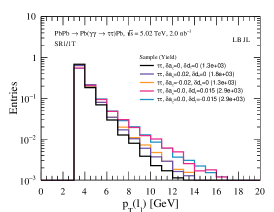
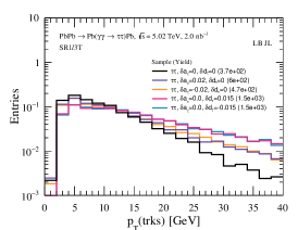
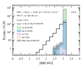
Figure 2: Distributions of lepton $p_{\text{T}}$ in SR$1\ell$1T (left) and the 3-track system $p_{\text{T}}$ in SR$1\ell$3T (center) for benchmark signals with various $\delta a_{\tau}$, $\delta d_{\tau}$ couplings. These are normalized to unit integral to illustrate shape changes with varying $\delta a_{\tau},\delta d_{\tau}$. The lepton–track azimuthal angle $|\Delta\phi(\ell,\text{trk})|$ in SR$1\ell$1T (right) is shown for backgrounds (filled) and signal $\delta a_{\tau}=\delta d_{\tau}=0$ (line), illustrating powerful discrimination against dilepton processes.

To record $\gamma\gamma\to\tau\tau$ events, dedicated UPC triggers are crucial for our proposal. With no other detector activity, the ditau system receives negligible transverse boost and each tau $p_{\text{T}}$ reaches a few to tens of GeV at most. Taus always decay to a neutrino $\nu_{\tau}$, which further dilutes the visible momenta, rendering usual hadronic tau triggers $p_{\text{T}}^{\text{$\tau$ jet}}\gtrsim 20$ GeV unfeasible Aaboud et al. (2017); ATLAS Collaboration (2017b). However, UPC events without pileup enable exceptionally low trigger thresholds by vetoing large sums over calorimeter transverse energy deposits $\sum E_{\text{T}}<50$ GeV ATLAS Collaboration (2019b). Other minimum bias triggers are also possible ATLAS Collaboration (2012, 2013). A recent UPC dimuon analysis additionally requires at least one track and no explicit $p_{\text{T}}$ requirement for the trigger muon ATLAS Collaboration (2016b). The light-by-light observation also considers ultralow $E_{\text{T}}>1$ GeV calorimeter cluster thresholds at trigger level ATLAS Collaboration (2019b), which can similarly benefit electrons.

We design our event selection around two objectives. First, we consider standard objects already deployed by ATLAS/CMS to efficiently reconstruct tau decays with the following branching fractions Tanabashi et al. (2018):

$$\mathcal{B}(\tau^{\pm}\to\ell^{\pm}\nu_{\ell}\nu_{\tau}) =35\%,$$ (7)

$$\mathcal{B}(\tau^{\pm}\to\pi^{\pm}\nu_{\tau}+\text{neutral pions}) =45.6\%,$$ (8)

$$\mathcal{B}(\tau^{\pm}\to\pi^{\pm}\pi^{\mp}\pi^{\pm}\nu_{\tau}+\text{neutral pions}) =19.4\%.$$ (9)

We develop signal regions (SR) targeting these decays based on expected signal rate and background mitigation strategies. We impose the lowest trigger and reconstruction thresholds $p_{\text{T}}^{e/\mu}>4.5/3$ GeV, $|\eta_{e/\mu}|<2.5/2.4$ supported by ATLAS/CMS ATLAS Collaboration (2018b); CMS Collaboration (2018a). Second, we optimize sensitivity to different couplings $\delta a_{\tau},\delta d_{\tau}$, where interfering SM and BSM amplitudes impact tau kinematics, which propagates to e.g. lepton $p_{\text{T}}$.

Dilepton analysis. Requiring two leptons is expected to give the highest signal-to-background $S/B$, with half being different flavor $e\mu$ free of $ee/\mu\mu$ backgrounds. But even using low $p_{\text{T}}^{e/\mu}$ thresholds, we find insufficient signal yields at 2 nb^-1 to pursue this further.

1 lepton + 1 track analysis (SR$1\ell$1T). This requires exactly 1 lepton and 1 other track that is not ‘matched’ to the lepton (the matched track is the highest $p_{\text{T}}$ track with $\Delta R(\ell,\text{track})<0.02$). Tracks must satisfy the standard requirements $p_{\text{T}}^{\text{track}}>500$ MeV and $|\eta^{\text{track}}|<$ 2.5. This topology targets the high branching ratio of the single charged pion decay mode and background suppression from lepton identification. The track also recovers events failing the dilepton analysis, in which a lepton is too soft to be reconstructed. We divide this SR into two bins $p_{\text{T}}^{e/\mu}\in[\leq 6],[>6]$ GeV to exploit shape differences shown in Fig. 2 (left). We require nonplanar lepton–track system $|\Delta\phi(\ell,\text{trk})|<3$ to suppress back-to-back $ee/\mu\mu$ processes, as demonstrated in Fig. 2 (right). We veto invariant masses $m_{\ell,\text{trk}}\not\in[3,3.2],[9,11]$ GeV to reject dilepton decays of $J/\psi$ and $\Upsilon$ resonances.

1 lepton + multitrack analysis (SR$1\ell$2/3T). We augment the previous analysis with 3 non-lepton-matched tracks. This targets the distinctive 3 charged pion decay. We also construct an orthogonal 2 tracks SR to recover misreconstructed 3-pion decays. The non-lepton-matched tracks are used to define the tau candidate as the vectorial sum of the tracks $p_{\tau}^{\text{tracks}}=\sum_{i}p^{\text{track}}_{i}$, whose $p_{\text{T}}$ distribution is shown in Fig. 2 (center) for SR$1\ell$3T. We find removing lepton identification significantly increases hadronic backgrounds.

Leptonic backgrounds are dominated by dielectron/dimuon production $\gamma\gamma\to\ell\ell,\ell\in[e,\mu]$. The single flavor cross-section is sizable $\sigma^{(\text{PbPb})}_{\gamma\gamma\to\ell\ell}=4.2\times 10^{5}$ nb, which includes a generator level $|\eta_{\ell}|<2.5$ requirement. The back-to-back leptons are suppressed by the $|\Delta\phi_{\ell\ell}|<3$ requirement, which we verify by generating 1 million events per flavor. Photon radiation from leptons $\ell\to\ell\gamma$ is only expected to modify the tails marginally. Track impact parameters exploiting displaced tau decays could further suppress this background.

Hadronic backgrounds arise from diquark production $\gamma\gamma\to q\bar{q}$ and we generate 1 million events for each of the 5 flavors. For $q\in[u,d,s]$ assuming massless quarks gives a cross-section $\sigma^{(\text{PbPb})}_{\gamma\gamma\to u\bar{u}\,(d\bar{d},s\bar{s})}=3.0\times 10^{5}$  ($1.9\times 10^{4}$) nb. Parton showering produces more tracks than tau decays, which we suppress using lepton isolation and requiring no more than 4 tracks at most. For $q\in[c,b]$, heavy flavor $B$ and $D$ mesons undergo semileptonic decays e.g. $D\to\pi^{0}\ell\nu$. The default MadGraph parameters assume massless charm quarks (which is conservative as a finite mass decreases cross-sections), yielding $\sigma^{(\text{PbPb})}_{\gamma\gamma\to c\bar{c}}=3.0\times 10^{5}$ nb. Bottom quarks assume finite mass resulting in a smaller cross-section $\sigma^{(\text{PbPb})}_{\gamma\gamma\to b\bar{b}}=1.5\times 10^{3}$ nb. The leptonic branching fraction $D\to\pi^{0}\ell\nu$ is of order a few percent so is under control, and is further suppressed by isolation.

Smaller potential backgrounds include $\gamma\gamma\to WW$ but the cross-section $\sigma^{(\text{PbPb})}_{\gamma\gamma\to WW}=14$ pb implies this is safely neglected. Exchange of digluon color singlets (Pomerons) also contributes to diquark backgrounds. These involve strong interactions and as the binding energy per nucleon is very small $\sim 8$ MeV d’Enterria and Lansberg (2010), the Pb ions emit more neutrons than QED processes, which can be vetoed by the Zero Degree Calorimeter ATLAS Collaboration (2007). Soft survival for Pomeron exchange is also lower d’Enterria and Lansberg (2010), which gives greater activity in the calorimeter and tracker, and are suppressed by our stringent exclusivity requirements.

Systematic uncertainties require LHC collaborations to reliably quantify, but we discuss expected sources and suggest control strategies. Experimental systematics from current UPC PbPb dimuon measurements have systematics of around 10%, dominated by luminosity and trigger ATLAS Collaboration (2016b). Systematics from lepton reconstruction are $p_{\text{T}}^{\ell}$-dependent and thus sensitive to $\delta a_{\tau}$. These are most significant at low $p_{\text{T}}$, but are currently determined in high luminosity proton collisions with challenging backgrounds from fakes ATLAS Collaboration (2019c, 2016c), and could be better controlled using clean $\gamma\gamma\to\ell\ell$ events.

Theoretical uncertainties are expected to be dominated by modeling of the photon flux, nuclear form factors and nucleon dissociation. Fortunately, these initial state effects are independent of QED process and final state. So, experimentalists could use a control sample of $\gamma\gamma\to\ell\ell$ events to constrain these universal nuclear systematics or eliminate them in a ratio analysis with dileptons $\sigma^{(\text{PbPb})}_{\gamma\gamma\to\tau\tau}/\sigma^{(\text{PbPb})}_{\gamma\gamma\to\ell\ell}$. Hadronic backgrounds are susceptible to uncertainties from modeling the parton shower, but are subdominant given $S/B\gg 1$ in our analyses.

IV Results & discussion

We now estimate the sensitivity of our analyses to modified tau moments $\delta a_{\tau},\delta d_{\tau}$. Assuming the observed data correspond to the SM expectation, we calculate

$$\chi^{2}=\frac{(S_{\text{SM+BSM}}-S_{\text{SM}})^{2}}{B+S_{\text{SM+BSM}}+(\zeta_{s}S_{\text{SM+BSM}})^{2}+(\zeta_{b}B)^{2}}.$$ (10)

Here, $B$ is the background rate, and $S_{\text{SM}}$ ($S_{\text{SM+BSM}}$) is the signal yield assuming SM couplings (nonzero $\delta a_{\tau},\delta d_{\tau}$). At $\mathcal{L}=2~{}$nb^-1, we find $S_{\text{SM}}=1280,B=7.6$ for SR$1\ell$1T before binning in $p_{\text{T}}^{\ell}$; $S_{\text{SM}}=520,B=15$ for SR$1\ell$2T; $S_{\text{SM}}=370,B=4$ for SR$1\ell$3T. We denote the relative signal (background) systematic uncertainties by $\zeta_{s}$ ($\zeta_{b}$) and study $\zeta_{s}=\zeta_{b}\in[5\%,10\%]$ as benchmarks. For simplicity, we assume identical $\zeta_{s}$ for all couplings, and combine the four SRs (SR$1\ell$1T has two $p_{\text{T}}^{\ell}$ bins) using $\chi^{2}=\sum\chi^{2}_{\text{SR}}$ assuming uncorrelated systematics. We define the 68% CL (95% CL) regions as couplings satisfying $\chi^{2}<1$ ($\chi^{2}<3.84$). Appendix B details cutflows for signals and backgrounds, and $\chi^{2}$ distributions.

Figure 3 summarizes our projected $a_{\tau}=a_{\tau,\,\mathrm{SM}}^{\text{pred}}+\delta a_{\tau}$ constraints (green) compared with existing measurements and predictions. Assuming the current dataset $\mathcal{L}=2$ nb^-1 with 10% systematics, we find $-0.0080<a_{\tau}<0.0046$ at 68% CL, surpassing DELPHI precision Abdallah et al. (2004) (blue) by a factor of three. Negative values of $\delta a_{\tau}$ are more difficult to constrain given destructive interference. We estimate prospects assuming halved systematics giving $-0.0022<a_{\tau}<0.0037$ (68% CL). A tenfold dataset increase for the High Luminosity LHC (HL-LHC) reduces this to $-0.00044<a_{\tau}<0.0032$ (68% CL), an order of magnitude improvement beyond DELPHI. Importantly, these advances start constraining the sign of $a_{\tau}$ and becomes comparable to the predicted SM central value for the first time.

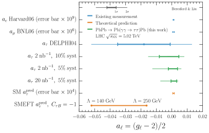
Figure 3: Summary of lepton anomalous magnetic moments $a_{\ell}=(g_{\ell}-2)/2$. Existing single-experiment measurements of $a_{e}$ Odom et al. (2006), $a_{\mu}$ Bennett et al. (2006), and $a_{\tau}$ Abdallah et al. (2004) are in blue. Our benchmark projections (green) assume 2 nb^-1 and 20 nb^-1 for 5% and 10% systematic uncertainties. For visual clarity, we inflate $1\sigma$ error bars on $a_{e}$ ($a_{\mu}$) measurements by $10^{9}$ ($10^{6}$), and $10^{4}$ for the SM prediction $a_{\tau}^{\text{pred}}$ (orange) Eidelman and Passera (2007). Collider constraints have thick (thin) lines denoting 68% CL, $1\sigma$ (95% CL, $\sim 2\sigma$). The SMEFT predictions Escribano and Masso (1993); Grzadkowski et al. (2010) from Eq. (4) with $C_{\tau B}=-1$ displays BSM scales $140<\Lambda<250$ GeV (thick orange).

Such precision indirectly probes BSM physics. In nature, compositeness can induce large and negative magnetic moments e.g. the neutron Tanabashi et al. (2018). As a benchmark, we fix $C_{\tau B}=-1,C_{\tau W}=0,\delta d_{\tau}=0$ in Eq. 3 to recast the DELPHI limit into a 95% CL exclusion of $\Lambda<140$ GeV. The orange line in Fig. 3 shows $140<\Lambda<250$ GeV, where our 2 nb^-1, 10% systematics proposal has $95\%$ CL sensitivity, surpassing DELPHI by 110 GeV. In suitable ultraviolet completions of SMEFT with composite leptons, one can interpret $\Lambda$ as the confinement scale of tau substructure Silverman and Shaw (1983). Nonetheless, our analyses are highly model-independent and we defer sensitivity to other BSM scenarios for future work. It would be interesting to correlate $a_{\tau}$ with models that simultaneously explain tensions in $a_{e}$ and $a_{\mu}$ Dutta and Mimura (2019); Davoudiasl and Marciano (2018); Bauer et al. (2019) or $B$-physics lepton universality tests LHCb Collaboration (2015); Belle Collaboration (2019); Allanach et al. (2016); Di Chiara et al. (2017); Biswas and Shaw (2019).

Lepton electric dipole moments are highly suppressed in the SM, arising only at four-loop $|d_{\tau}^{\text{pred}}|\sim(m_{\tau}/m_{e})|d_{e}^{\text{pred}}|\sim 10^{-33}~{}e$ cm Pospelov and Khriplovich (1991). Additional CP violation in the lepton sector can enhance this, such as neutrino mixing Ng and Ng (1996), or other BSM physics parameterized by $\varphi$ in Eq. 4. Our projected 95% CL sensitivity on $d_{\tau}=(e/m_{\tau})\delta d_{\tau}$ is $|d_{\tau}|<3.4\times 10^{-17}~{}e$ cm, assuming $\delta a_{\tau}=0$ with 2 nb^-1, 10% systematics. This is an order of magnitude better than DELPHI $|d_{\tau}|<3.7\times 10^{-16}~{}e$ cm Abdallah et al. (2004) and competitive with Belle Inami et al. (2003).

Our proposal opens numerous avenues for extension. Lowering lepton/track thresholds to increase statistics would enable more optimized differential or multivariate analyses. Recently, ATLAS considered tracks matched to lepton candidates failing quality requirements, allowing $p_{\text{T}}^{\text{track}}(e/\mu)>1/2$ GeV ATLAS Collaboration (2019a). Moreover the 500 MeV track threshold is conservative given $p_{\text{T}}^{\text{track}}>100$ MeV is successfully used in ATLAS ATLAS Collaboration (2019b). Reconstructing soft calorimeter clusters could enable hadron/electron identification, or using neutral pions to improve tau momentum resolution. Proposed timing detectors may offer more robust particle identification in ATLAS/CMS CMS Collaboration (2017) while ALICE already has such capabilities Yu (2013). Ultimate $a_{\tau}$ precision requires a coordinated worldwide program led by LHC efforts combined with proton–lead collisions at $\sqrt{s_{\text{NN}}}=8.76$ TeV, Relativistic Heavy Ion Collider (RHIC), and lepton colliders.

To summarize, we proposed a strategy of lepton plus track(s) analyses to surpass LEP constraints on tau electromagnetic moments using heavy ion data already recorded by the LHC. The clean photon collision events provide excellent opportunities to optimize low momentum reconstruction and control systematics further. We encourage LHC collaborations to open these cornerstone measurements and precision pathways to new physics.

Acknowledgements—We thank the hospitality of the LHC Forward and Diffractive Physics Workshop at CERN, where part of this work began. We are grateful to Luca Ambroz, Bill Balunas, Alan Barr, Mikkel Bjørn, Barak Gruberg, Lucian Harland-Lang, Simon Knapen, Santiago Paredes, Hannah Pullen, Hayden Smith, Beojan Stanislaus, Gabija Žemaitytė and Miha Zgubič for helpful discussions. LB is supported by a Junior Research Fellowship at St John’s College, Oxford. JL is supported by an STFC Postgraduate Studentship at Oxford, where this work started, and the Grainger Fellowship.

Appendix A Simulation validation

We present additional material to validate the technical implementation of our simulation setup models the intended physics effects within the scope of our work. This includes the photon flux we implemented in MadGraph 2.6.5 Alwall et al. (2011, 2014), and the interface with SMEFTsim Brivio et al. (2017) for BSM modifications and interference with the SM.

Figure 4 displays generator level differential distributions of $p_{\text{T}}(\tau)$ for $\gamma\gamma\to\tau\tau$ considering various photon fluxes from protons and lead (Pb) beams. The distribution generated in MadGraph with Pb uses our custom implementation of Pb ion photon flux. We validate this with the corresponding distribution generated in Superchic 3.02 Harland-Lang et al. (2019b). The latter includes a full treatment of nuclear effects that are neglected by the factorized prescription in MadGraph. These two distributions are in reasonable agreement for the scope of our work. Also shown are the corresponding distributions for proton beams. This illustrates that the impact of a nucleus with comparatively finite size is to soften the $p_{\text{T}}(\tau)$ spectrum compared to using proton beams.

Figure 5 shows the impact of the interference behavior on the inclusive cross-sections of $\sigma_{\gamma\gamma\to\tau\tau}^{(PbPb)}$ for coupling variations $\delta a_{\tau}$ using SMEFTsim. We account for the interference between SM and BSM $\gamma\gamma\to\tau\tau$ diagrams in the matrix element $\mathcal{M}$ squared

$$|\mathcal{M}|^{2} =\left|\mathcal{M}_{\text{SM}}+\mathcal{M}_{\text{BSM}}^{(1)}+\mathcal{M}_{\text{BSM}}^{(2)}\right|^{2}$$ (11)

$$=\begin{gathered}\includegraphics{figs/feynGraphs/amplitudeSq.pdf}\end{gathered}.$$ (13)

A BSM coupling is represented by $\bullet$ in the matrix element diagrams. Cross-sections featuring just the diagrams with only 1 BSM coupling (blue triangle) and only 2 BSM couplings (blue square) are shown in Fig. 5, which correspond to the amplitudes $\mathcal{M}_{\text{BSM}}^{(1)}$ and $\mathcal{M}_{\text{BSM}}^{(2)}$ respectively. As $\delta a_{\tau}$ deviates from zero in the negative direction, $\sigma_{\gamma\gamma\to\tau\tau}^{\text{(PbPb)}}$ falls to a minimum at $\delta a_{\tau}\simeq-0.04$ due to destructive interference from $\mathcal{M}_{\text{BSM}}^{(1)}$. Then, the constructively interfering $\mathcal{M}_{\text{BSM}}^{(2)}$ term begins to dominate for more negative $\delta a_{\tau}$ values and $\sigma_{\gamma\gamma\to\tau\tau}^{\text{(PbPb)}}$ rises again.

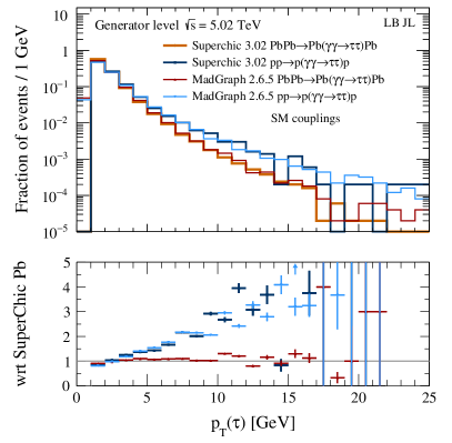
Figure 4: Unit normalized generator level tau $p_{\text{T}}$ distributions for $\gamma\gamma\to\tau\tau$ using SM couplings. These are generated in Superchic 3.02, which includes a full treatment of nuclear effects for lead (Pb) ions (orange). Also shown is the corresponding sample with protons (dark blue). The MadGraph 2.6.5 samples uses a factorized photon flux prescription for protons (light blue) and our implementation of Pb ion flux (red). The ratio panel is with respect to the Superchic Pb ions sample.

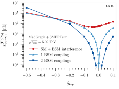
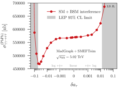
Figure 5: Generator level cross-sections for $\gamma\gamma\to\tau\tau$ sourced by our implementation of the Pb photon flux in MadGraph. This is interfaced with SMEFTsim for BSM coupling variations in $\delta a_{\tau}$ defined in Eq. 4 of the main text, fixing $\delta d_{\tau}=0$ at $\sqrt{s_{\text{NN}}}=5.02$ TeV. Left shows the contribution from only 1 BSM coupling (light blue triangles), 2 BSM couplings (dark blue squares), and their combined interference with the SM (red circles). The markers indicate the sampled points from $\delta a_{\tau}$. Right zooms in to the $\delta a_{\tau}$ values near zero with gray regions denoting the 95% CL exclusion by DELPHI, where the horizontal axis is linear scale for $\delta a_{\tau}\in[-0.001,0.001]$ and logarithmic elsewhere.

Appendix B Cutflows and $\chi^{2}$ distributions

We provide technical material supporting the results presented in the main text. These include signal and background counts after sequentially applying kinematic requirements (cutflow), and $\chi^{2}$ distributions as functions of $\delta a_{\tau}$ and $\delta d_{\tau}$ used to derive the final constraints.

Requirement	$\tau\tau$ $(0,0)$	$\tau\tau$ $(0.005,0)$	$\tau\tau$ $(-0.01,0)$	$\mu\mu$	$ee$	$bb$	$cc$	$ss$	$uu$	$dd$
1 lepton + 1 track analysis (SR$1\ell$1T)
$\sigma\times\mathcal{L}$	$1139800$	$1195060$	$1056400$	$844080$	$844080$	$2999$	$604080$	$37754$	$604080$	$37754$
$\sigma\times\mathcal{L}\times\epsilon_{\text{filter}}$	$241140$	$253920$	$226300$	$844080$	$844080$	$2999$	$604080$	$37754$	$604080$	$37754$
$1\ell$ plus 1 track	$20492.2$	$21619.3$	$19348.4$	$263443$	$3299.3$	$5.4$	$2905.0$	$0.3$	$5.4$	$0.2$
$p_{\text{T}}^{e/\mu}>4.5/3~{}\text{GeV}$, $|\eta^{e/\mu}|<2.5/2.4$	$3659.9$	$3882.7$	$3582.8$	$79043$	$3118.9$	$1.1$	$4.8$	$0.0$	$0.0$	$0.0$
2 tracks, $p_{\text{T}}^{\text{trk}}>0.5~{}\text{GeV}$, $|\eta^{\text{trk}}|<$ 2.5	$3324.5$	$3535.9$	$3256.9$	$78973$	$3117.8$	$1.0$	$3.0$	$0.0$	$0.0$	$0.0$
$|\Delta\phi(\ell,\text{trk})|<3$	$1519.7$	$1605.7$	$1468.3$	$0.9$	$5.3$	$0.7$	$1.8$	$0.0$	$0.0$	$0.0$
$m_{\ell,\text{trk}}\not\in\{[3,3.2],[9,11]\}$ GeV	$1275.1$	$1353.6$	$1242.3$	$0.9$	$5.3$	$0.2$	$1.2$	$0.0$	$0.0$	$0.0$
$p_{\text{T}}^{\ell}\leq 6.0~{}\rm{GeV}$	$1197.7$	$1262.3$	$1154.7$	$0.9$	$0.0$	$0.2$	$1.2$	$0.0$	$0.0$	$0.0$
$p_{\text{T}}^{\ell}>6.0~{}\rm{GeV}$	$77.3$	$91.3$	$87.6$	$0.0$	$5.3$	$0.0$	$0.0$	$0.0$	$0.0$	$0.0$
1 lepton + multitrack analysis (SR$1\ell$2/3T)
$\sigma\times\mathcal{L}$	$1139800$	$1195060$	$1056400$	$844080$	$844080$	$2999$	$604080$	$37754$	$604080$	$37754$
$\sigma\times\mathcal{L}\times\epsilon_{\text{filter}}$	$241140$	$253920$	$226300$	$844080$	$844080$	$2999$	$604080$	$37754$	$604080$	$37754$
$1\ell$ plus 2 or 3 tracks	$5945.1$	$6260.1$	$5572.2$	$33.8$	$23.2$	$43.8$	$8056.6$	$5.4$	$132.9$	$6.8$
$p_{\text{T}}^{e/\mu}>4.5/3~{}\text{GeV}$, $|\eta^{e/\mu}|<2.5/2.4$	$1010.0$	$1073.3$	$978.6$	$12.2$	$4.2$	$1.8$	$13.3$	$0.0$	$0.0$	$0.0$
3 tracks, $p_{\text{T}}^{\text{trk}}>0.5~{}\text{GeV}$, $|\eta|^{\text{trk}}<$ 2.5	$519.9$	$548.1$	$485.8$	$5.6$	$4.2$	$0.8$	$4.8$	$0.0$	$0.0$	$0.0$
4 tracks, $p_{\text{T}}^{\text{trk}}>0.5~{}\text{GeV}$, $|\eta|^{\text{trk}}<$ 2.5	$370.5$	$398.3$	$381.1$	$0.0$	$0.0$	$0.4$	$3.6$	$0.0$	$0.0$	$0.0$

Table 1: Cutflow of yields after each requirement applied sequentially, normalized to $\mathcal{L}=2$ nb^-1 for the different analyses. For the $\gamma\gamma\to\tau\tau$ signal processes, we show these for benchmark points with parameter values labeled by $(\delta a_{\tau},\delta d_{\tau})$ displayed in the column header. Backgrounds are shown for various dilepton $\mu\mu,ee$ and diquark where the letters denote the flavor. The initial value in each cutflow is the cross-section $\sigma$ times luminosity $\mathcal{L}$, followed by the efficiency $\epsilon_{\text{filter}}$ of the filter applied at generator level to the $\gamma\gamma\to\tau\tau$ samples.

Table 1 presents the set of cutflows for the different analyses, sequentially displaying the yields normalized to 2 nb^-1 after each signal region requirement. Three benchmark signals are shown for the $\gamma\gamma\to\tau\tau$ samples at the SM values $(\delta a_{\tau},\delta d_{\tau})=(0,0)$ and for values near the threshold of 68% CL sensitivity $(\delta a_{\tau},\delta d_{\tau})\in\{(0.005,0),(-0.01,0)\}$.

Figure 6 shows the $\chi^{2}$ distributions as a function of $\delta a_{\tau}$ and $\delta d_{\tau}$ assuming the other is zero for separate signal regions. These are shown assuming 10% systematics, 2 nb^-1 to allow comparison of constraining power between the different analyses presented in the main text.

Figure 7 displays the combined $\chi^{2}=\sum_{i}\chi_{i}^{2}$ distributions. The combined $\chi^{2}$ distributions are shown for 10% systematics at 2 nb^-1 together with prospects using 5% systematics and extrapolation to 20 nb^-1. The red lines show the results from combining the three track SRs. The final combined $\chi^{2}$ for the results in the main text take the green lines, which combine all four signal regions (SR$1\ell$1T is divided into two orthogonal $p_{\text{T}}^{\ell}$ bins). The final 68% CL and 95% CL intervals are defined by where the $\chi^{2}$ distributions intersect with $\chi^{2}=1$ and $\chi^{2}=3.84$ respectively.

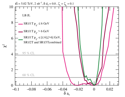
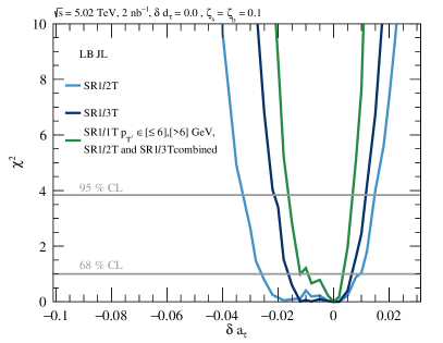
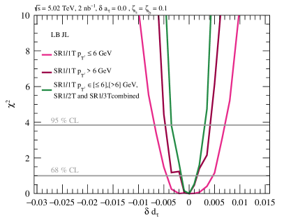
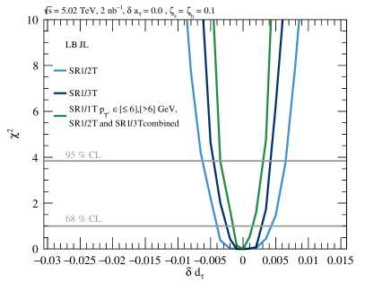
Figure 6: The $\chi^{2}$ distributions as a function of $\delta a_{\tau}$ assuming $\delta d_{\tau}=0$ (upper), and $\delta a_{\tau}$ assuming $\delta d_{\tau}=0$ (lower) are displayed for 10% systematics at $\mathcal{L}=2$ nb^-1. Left shows the results from the SR$1\ell$1T regions and the impact of binning in $p_{\text{T}}^{\ell}$. Right shows the results from the SR$1\ell$2/3T regions. The four signal region combined $\chi^{2}$ is shown by the green line for reference. The gray horizontal lines correspond to 68% CL ($\chi^{2}$=1) and 95% CL ($\chi^{2}$=3.84)

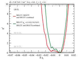
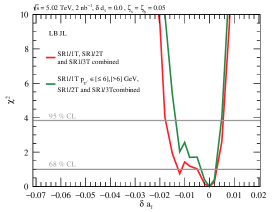
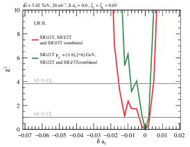
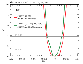
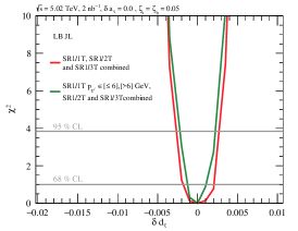
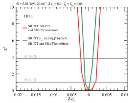
Figure 7: The $\chi^{2}$ distributions as a function of $\delta a_{\tau}$ assuming $\delta d_{\tau}=0$ (upper), and $\delta a_{\tau}$ assuming $\delta d_{\tau}=0$ (lower). These are displayed for 10% (left), 5% (centre) systematics at $\mathcal{L}=2$ nb^-1, and 5% systematics result extrapolated to $\mathcal{L}=20$ nb^-1 (right). The combined $\chi^{2}$ for all three track SRs is shown by the red line, while the impact of dividing SR$1\ell$1T into two orthogonal $p_{\text{T}}^{\ell}$ bins is shown by the green line. The gray horizontal lines correspond to 68% CL ($\chi^{2}$=1) and 95% CL ($\chi^{2}$=3.84)

References

- Odom et al. (2006) B. Odom, D. Hanneke, B. D’Urso, and G. Gabrielse, “New Measurement of the Electron Magnetic Moment Using a One-Electron Quantum Cyclotron,” Phys. Rev. Lett. 97, 030801 (2006).
- Hanneke et al. (2011) D. Hanneke, S. Fogwell Hoogerheide, and G. Gabrielse, “Cavity Control of a Single-Electron Quantum Cyclotron: Measuring the Electron Magnetic Moment,” Phys. Rev. A83, 052122 (2011), arXiv:1009.4831 [physics.atom-ph] .
- Bouchendira et al. (2011) R. Bouchendira, P. Cladé, S. Guellati-Khélifa, F. Nez, and F. Biraben, “New Determination of the Fine Structure Constant and Test of the Quantum Electrodynamics,” Phys. Rev. Lett. 106, 080801 (2011).
- Aoyama et al. (2012a) T. Aoyama, M. Hayakawa, T. Kinoshita, and M. Nio, “Tenth-Order QED Contribution to the Electron g-2 and an Improved Value of the Fine Structure Constant,” Phys. Rev. Lett. 109, 111807 (2012a), arXiv:1205.5368 [hep-ph] .
- Parker et al. (2018) R. H. Parker, C. Yu, W. Zhong, B. Estey, and H. Müller, “Measurement of the fine-structure constant as a test of the Standard Model,” Science 360, 191–195 (2018).
- Bennett et al. (2006) G. W. Bennett et al. (Muon g-2), “Final Report of the Muon E821 Anomalous Magnetic Moment Measurement at BNL,” Phys. Rev. D 73, 072003 (2006), arXiv:hep-ex/0602035 [hep-ex] .
- Aoyama et al. (2012b) T. Aoyama, M. Hayakawa, T. Kinoshita, and M. Nio, “Complete Tenth-Order QED Contribution to the Muon g-2,” Phys. Rev. Lett. 109, 111808 (2012b), arXiv:1205.5370 [hep-ph] .
- Keshavarzi et al. (2018) A. Keshavarzi, D. Nomura, and T. Teubner, “Muon and : a new data-based analysis,” Phys. Rev. D97, 114025 (2018), arXiv:1802.02995 [hep-ph] .
- Martin and Wells (2001) Stephen P. Martin and James D. Wells, “Muon Anomalous Magnetic Dipole Moment in Supersymmetric Theories,” Phys. Rev. D64, 035003 (2001), arXiv:hep-ph/0103067 [hep-ph] .
- Czarnecki and Marciano (2001) Andrzej Czarnecki and William J. Marciano, “The Muon anomalous magnetic moment: A Harbinger for ’new physics’,” Phys. Rev. D64, 013014 (2001), arXiv:hep-ph/0102122 [hep-ph] .
- Hagiwara et al. (2011) K. Hagiwara, R. Liao, A. D. Martin, D. Nomura, and T. Teubner, “ and re-evaluated using new precise data,” J. Phys. G 38, 085003 (2011), arXiv:1105.3149 [hep-ph] .
- Ajaib et al. (2015) M. Adeel Ajaib, B. Dutta, T. Ghosh, I. Gogoladze, and Q. Shafi, “Neutralinos and sleptons at the LHC in light of muon ,” Phys. Rev. D 92, 075033 (2015), arXiv:1505.05896 [hep-ph] .
- Grange et al. (2015) J. Grange et al. (Muon g-2), “Muon (g-2) Technical Design Report,” (2015), arXiv:1501.06858 [physics.ins-det] .
- Abe et al. (2019) M. Abe et al., “A New Approach for Measuring the Muon Anomalous Magnetic Moment and Electric Dipole Moment,” (2019), arXiv:1901.03047 [physics.ins-det] .
- Silverman and Shaw (1983) D. J. Silverman and G. L. Shaw, “Limits on the Composite Structure of the Tau Lepton and Quarks From Anomalous Magnetic Moment Measurements in Annihilation,” Phys. Rev. D27, 1196 (1983).
- Abdallah et al. (2004) J. Abdallah et al. (DELPHI), “Study of tau-pair production in photon-photon collisions at LEP and limits on the anomalous electromagnetic moments of the tau lepton,” Eur. Phys. J. C35, 159–170 (2004), arXiv:hep-ex/0406010 [hep-ex] .
- Tanabashi et al. (2018) M. Tanabashi et al. (Particle Data Group), “Review of Particle Physics,” Phys. Rev. D98, 030001 (2018).
- Eidelman and Passera (2007) S. Eidelman and M. Passera, “Theory of the tau lepton anomalous magnetic moment,” Mod. Phys. Lett. A22, 159–179 (2007), arXiv:hep-ph/0701260 [hep-ph] .
- Dutta and Mimura (2019) B. Dutta and Y. Mimura, “Electron with flavor violation in MSSM,” Phys. Lett. B790, 563–567 (2019), arXiv:1811.10209 [hep-ph] .
- Davoudiasl and Marciano (2018) H. Davoudiasl and W. J. Marciano, “Tale of two anomalies,” Phys. Rev. D98, 075011 (2018), arXiv:1806.10252 [hep-ph] .
- Bauer et al. (2019) M. Bauer, M. Neubert, S. Renner, M. Schnubel, and A. Thamm, “Axion-like particles, lepton-flavor violation and a new explanation of and ,” (2019), arXiv:1908.00008 [hep-ph] .
- LHCb Collaboration (2015) LHCb Collaboration, “Measurement of the ratio of branching fractions ,” Phys. Rev. Lett. 115, 111803 (2015), [Erratum: Phys. Rev. Lett.115, no.15, 159901(2015)], arXiv:1506.08614 [hep-ex] .
- Belle Collaboration (2019) Belle Collaboration, “Measurement of and with a semileptonic tagging method,” (2019), arXiv:1904.08794 [hep-ex] .
- Allanach et al. (2016) B. Allanach, F. S. Queiroz, A. Strumia, and S. Sun, “ models for the LHCb and muon anomalies,” Phys. Rev. D93, 055045 (2016), [Erratum: Phys. Rev.D95,no.11,119902(2017)], arXiv:1511.07447 [hep-ph] .
- Di Chiara et al. (2017) S. Di Chiara, A. Fowlie, S. Fraser, C. Marzo, L. Marzola, M. Raidal, and C. Spethmann, “Minimal flavor-changing models and muon after the measurement,” Nucl. Phys. B923, 245–257 (2017), arXiv:1704.06200 [hep-ph] .
- Biswas and Shaw (2019) A. Biswas and A. Shaw, “Reconciling dark matter, anomalies and in an scenario,” JHEP 05, 165 (2019), arXiv:1903.08745 [hep-ph] .
- del Aguila et al. (1991) F. del Aguila, F. Cornet, and J. I. Illana, “The possibility of using a large heavy-ion collider for measuring the electromagnetic properties of the tau lepton,” Physics Letters B 271, 256 – 260 (1991).
- Koksal et al. (2018) M. Koksal, A. A. Billur, A. Gutiérrez-Rodríguez, and M. A. Hernández-Ruíz, “Model-independent sensitivity estimates for the electromagnetic dipole moments of the -lepton at the CLIC,” Phys. Rev. D98, 015017 (2018), arXiv:1804.02373 [hep-ph] .
- Howard et al. (2018) J. N. Howard, A. Rajaraman, R. Riley, and T. M. P. Tait, “The Magnetic Dipole Moment at Future Lepton Colliders,” (2018), arXiv:1810.09570 [hep-ph] .
- Koksal (2018) M. Koksal, “Search for the electromagnetic moments of the lepton in photon-photon collisions at the LHeC and the FCC-he,” (2018), arXiv:1809.01963 [hep-ph] .
- Gutiérrez-Rodríguez et al. (2019) A. Gutiérrez-Rodríguez, M. Köksal, A. A. Billur, and M. A. Hernández-Ruíz, “Feasibility at the LHC, FCC-he and CLIC for sensitivity estimates on anomalous -lepton couplings,” (2019), arXiv:1903.04135 [hep-ph] .
- Fael et al. (2014) M. Fael, L. Mercolli, and M. Passera, “Towards a determination of the tau lepton dipole moments,” Nucl. Phys. Proc. Suppl. 253-255, 103–106 (2014), arXiv:1301.5302 [hep-ph] .
- Eidelman et al. (2016) S. Eidelman, D. Epifanov, M. Fael, L. Mercolli, and M. Passera, “ dipole moments via radiative leptonic decays,” JHEP 03, 140 (2016), arXiv:1601.07987 [hep-ph] .
- Chen and Wu (2018) X. Chen and Y. Wu, “Search for the Electric Dipole Moment and anomalous magnetic moment of the tau lepton at tau factories,” (2018), arXiv:1803.00501 [hep-ph] .
- Samuel and Li (1994) M. A. Samuel and G. Li, “How to measure the magnetic moment of the tau lepton,” International Journal of Theoretical Physics 33, 1471–1477 (1994).
- Hayreter and Valencia (2013) Alper Hayreter and German Valencia, “Constraining -lepton dipole moments and gluon couplings at the LHC,” Phys. Rev. D88, 013015 (2013), [Erratum: Phys. Rev.D91,no.9,099902(2015)], arXiv:1305.6833 [hep-ph] .
- Atag and Billur (2010) S. Atag and A. A. Billur, “Possibility of Determining Lepton Electromagnetic Moments in Process at the CERN-LHC,” JHEP 11, 060 (2010), arXiv:1005.2841 [hep-ph] .
- Galon et al. (2016) I. Galon, A. Rajaraman, and T. M. P. Tait, “ as a probe of the magnetic dipole moment,” JHEP 12, 111 (2016), arXiv:1610.01601 [hep-ph] .
- Fomin et al. (2019) A. S. Fomin, A. Yu Korchin, A. Stocchi, S. Barsuk, and P. Robbe, “Feasibility of -lepton electromagnetic dipole moments measurement using bent crystal at the LHC,” JHEP 03, 156 (2019), arXiv:1810.06699 [hep-ph] .
- Fu et al. (2019) J. Fu, M. A. Giorgi, L. Henry, D. Marangotto, F. Martínez Vidal, A. Merli, N. Neri, and J. Ruiz Vidal, “Novel Method for the Direct Measurement of the Lepton Dipole Moments,” Phys. Rev. Lett. 123, 011801 (2019), arXiv:1901.04003 [hep-ex] .
- ATLAS Collaboration (2018a) ATLAS Collaboration, Back-to-back electron-muon pair in an ultra-peripheral collision recorded with the ATLAS detector, Tech. Rep. (2018).
- ATLAS Collaboration (2018b) ATLAS Collaboration, “Search for electroweak production of supersymmetric states in scenarios with compressed mass spectra at TeV with the ATLAS detector,” Phys. Rev. D97, 052010 (2018b), arXiv:1712.08119 [hep-ex] .
- CMS Collaboration (2018a) CMS Collaboration, “Search for new physics in events with two soft oppositely charged leptons and missing transverse momentum in proton-proton collisions at 13 TeV,” Phys. Lett. B782, 440–467 (2018a), arXiv:1801.01846 [hep-ex] .
- ATLAS Collaboration (2019a) ATLAS Collaboration, Searches for electroweak production of supersymmetric particles with compressed mass spectra in TeV collisions with the ATLAS detector, Tech. Rep. ATLAS-CONF-2019-014 (2019).
- Piotrzkowski (2001) K. Piotrzkowski, “Tagging two photon production at the CERN LHC,” Phys. Rev. D63, 071502 (2001), arXiv:hep-ex/0009065 [hep-ex] .
- Albrow et al. (2009) M. G. Albrow et al. (FP420 R & D), “The FP420 R & D Project: Higgs and New Physics with forward protons at the LHC,” JINST 4, T10001 (2009), arXiv:0806.0302 [hep-ex] .
- de Favereau de Jeneret et al. (2009) J. de Favereau de Jeneret, V. Lemaitre, Y. Liu, S. Ovyn, T. Pierzchala, K. Piotrzkowski, X. Rouby, N. Schul, and M. Vander Donckt, “High energy photon interactions at the LHC,” (2009), arXiv:0908.2020 [hep-ph] .
- d’Enterria and da Silveira (2013) D. d’Enterria and G. G. da Silveira, “Observing light-by-light scattering at the Large Hadron Collider,” Phys. Rev. Lett. 111, 080405 (2013), [Erratum: Phys. Rev. Lett.116,no.12,129901(2016)], arXiv:1305.7142 [hep-ph] .
- ATLAS Collaboration (2017a) ATLAS Collaboration, “Evidence for light-by-light scattering in heavy-ion collisions with the ATLAS detector at the LHC,” Nature Phys. 13, 852–858 (2017a), arXiv:1702.01625 [hep-ex] .
- CMS Collaboration (2018b) CMS Collaboration, “Evidence for light-by-light scattering and searches for axion-like particles in ultraperipheral PbPb collisions at 5.02 TeV,” (2018b), arXiv:1810.04602 [hep-ex] .
- ATLAS Collaboration (2019b) ATLAS Collaboration, “Observation of light-by-light scattering in ultraperipheral Pb+Pb collisions with the ATLAS detector,” Phys. Rev. Lett. 123, 052001 (2019b), arXiv:1904.03536 [hep-ex] .
- ATLAS Collaboration (2018c) ATLAS Collaboration, “Measurement of the exclusive process in proton-proton collisions at TeV with the ATLAS detector,” Phys. Lett. B777, 303–323 (2018c), arXiv:1708.04053 [hep-ex] .
- ATLAS Collaboration (2016a) ATLAS Collaboration, “Measurement of exclusive production and search for exclusive Higgs boson production in collisions at TeV using the ATLAS detector,” Phys. Rev. D94, 032011 (2016a), arXiv:1607.03745 [hep-ex] .
- CMS Collaboration (2012) CMS Collaboration, “Search for exclusive or semi-exclusive photon pair production and observation of exclusive and semi-exclusive electron pair production in collisions at TeV,” JHEP 11, 080 (2012), arXiv:1209.1666 [hep-ex] .
- CMS Collaboration (2016) CMS Collaboration, “Evidence for exclusive production and constraints on anomalous quartic gauge couplings in collisions at and 8 TeV,” JHEP 08, 119 (2016), arXiv:1604.04464 [hep-ex] .
- ATLAS Collaboration (2016b) ATLAS Collaboration, Measurement of high-mass dimuon pairs from ultraperipheral lead-lead collisions at TeV with the ATLAS detector , Tech. Rep. ATLAS-CONF-2016-025 (2016).
- Chapon et al. (2010) E. Chapon, C. Royon, and O. Kepka, “Anomalous quartic , , and trilinear couplings in two-photon processes at high luminosity at the LHC,” Phys. Rev. D81, 074003 (2010), arXiv:0912.5161 [hep-ph] .
- Fichet et al. (2014) S. Fichet, G. von Gersdorff, O. Kepka, B. Lenzi, C. Royon, and M. Saimpert, “Probing new physics in diphoton production with proton tagging at the Large Hadron Collider,” Phys. Rev. D89, 114004 (2014), arXiv:1312.5153 [hep-ph] .
- Ellis et al. (2017) J. Ellis, N. E. Mavromatos, and T. You, “Light-by-Light Scattering Constraint on Born-Infeld Theory,” Phys. Rev. Lett. 118, 261802 (2017), arXiv:1703.08450 [hep-ph] .
- Knapen et al. (2017) S. Knapen, T. Lin, H. K. Lou, and T. Melia, “Searching for Axionlike Particles with Ultraperipheral Heavy-Ion Collisions,” Phys. Rev. Lett. 118, 171801 (2017), arXiv:1607.06083 [hep-ph] .
- Baldenegro et al. (2018) C. Baldenegro, S. Fichet, G. von Gersdorff, and C. Royon, “Searching for axion-like particles with proton tagging at the LHC,” JHEP 06, 131 (2018), arXiv:1803.10835 [hep-ph] .
- Ohnemus et al. (1994) J. Ohnemus, T. F. Walsh, and P. M. Zerwas, “gamma gamma production of nonstrongly interacting SUSY particles at hadron colliders,” Phys. Lett. B328, 369–373 (1994), arXiv:hep-ph/9402302 [hep-ph] .
- Schul and Piotrzkowski (2008) N. Schul and K. Piotrzkowski, “Detection of two-photon exclusive production of supersymmetric pairs at the LHC,” Nucl. Phys. Proc. Suppl. 179-180, 289–297 (2008), arXiv:0806.1097 [hep-ph] .
- Harland-Lang et al. (2012) L. A. Harland-Lang, C. H. Kom, K. Sakurai, and W. J. Stirling, “Measuring the masses of a pair of semi-invisibly decaying particles in central exclusive production with forward proton tagging,” Eur. Phys. J. C72, 1969 (2012), arXiv:1110.4320 [hep-ph] .
- Beresford and Liu (2018) L. Beresford and J. Liu, “Photon collider search strategy for sleptons and dark matter at the LHC,” (2018), arXiv:1811.06465 [hep-ph] .
- Harland-Lang et al. (2019a) L. A. Harland-Lang, V. A. Khoze, M. G. Ryskin, and M. Tasevsky, “LHC Searches for Dark Matter in Compressed Mass Scenarios: Challenges in the Forward Proton Mode,” JHEP 04, 010 (2019a), arXiv:1812.04886 [hep-ph] .
- Bruce et al. (2018) R. Bruce et al., “New physics searches with heavy-ion collisions at the LHC,” (2018), arXiv:1812.07688 [hep-ph] .
- Escribano and Masso (1993) R. Escribano and E. Masso, “New bounds on the magnetic and electric moments of the tau lepton,” Phys. Lett. B301, 419–422 (1993).
- Grzadkowski et al. (2010) B. Grzadkowski, M. Iskrzynski, M. Misiak, and J. Rosiek, “Dimension-Six Terms in the Standard Model Lagrangian,” JHEP 10, 085 (2010), arXiv:1008.4884 [hep-ph] .
- Brodsky et al. (1971) S. J. Brodsky, T. Kinoshita, and H. Terazawa, “Two Photon Mechanism of Particle Production by High-Energy Colliding Beams,” Phys. Rev. D4, 1532–1557 (1971).
- Tupper and Samuel (1981) G. Tupper and M. A. Samuel, “ pair production in two-photon collisions and the magnetic moment of the bosons,” Phys. Rev. D 23, 1933–1939 (1981).
- Brivio et al. (2017) I. Brivio, Y. Jiang, and M. Trott, “The SMEFTsim package, theory and tools,” JHEP 12, 070 (2017), arXiv:1709.06492 [hep-ph] .
- Alloul et al. (2014) A. Alloul, N. D. Christensen, C. Degrande, C. Duhr, and B. Fuks, “FeynRules 2.0 - A complete toolbox for tree-level phenomenology,” Comput. Phys. Commun. 185, 2250–2300 (2014), arXiv:1310.1921 [hep-ph] .
- Alwall et al. (2011) J. Alwall, M. Herquet, F. Maltoni, O. Mattelaer, and T. Stelzer, “MadGraph 5 : Going Beyond,” JHEP 06, 128 (2011), arXiv:1106.0522 [hep-ph] .
- Alwall et al. (2014) J. Alwall et al., “The automated computation of tree-level and next-to-leading order differential cross sections, and their matching to parton shower simulations,” JHEP 07, 079 (2014), arXiv:1405.0301 [hep-ph] .
- Budnev et al. (1975) V. M. Budnev, I. F. Ginzburg, G. V. Meledin, and V. G. Serbo, “The Two photon particle production mechanism. Physical problems. Applications. Equivalent photon approximation,” Phys. Rept. 15, 181–281 (1975).
- d’Enterria and Lansberg (2010) D. d’Enterria and J.-P. Lansberg, “Study of Higgs boson production and its b anti-b decay in gamma-gamma processes in proton-nucleus collisions at the LHC,” Phys. Rev. D81, 014004 (2010), arXiv:0909.3047 [hep-ph] .
- Jackson (1999) J. D. Jackson, Classical electrodynamics; 3rd ed. (Wiley, New York, NY, 1999).
- Zhang and Jin (1996) S. Zhang and J.M. Jin, Computation of Special Functions, A Wiley-Interscience publication (Wiley, 1996).
- Harland-Lang et al. (2019b) L. A. Harland-Lang, V. A. Khoze, and M. G. Ryskin, “Exclusive LHC physics with heavy ions: SuperChic 3,” Eur. Phys. J. C79, 39 (2019b), arXiv:1810.06567 [hep-ph] .
- Sjostrand et al. (2008) T. Sjostrand, S. Mrenna, and P. Z. Skands, “A Brief Introduction to PYTHIA 8.1,” Comput. Phys. Commun. 178, 852–867 (2008), arXiv:0710.3820 [hep-ph] .
- de Favereau et al. (2014) J. de Favereau, C. Delaere, P. Demin, A. Giammanco, V. Lemaître, A. Mertens, and M. Selvaggi (DELPHES 3), “DELPHES 3, A modular framework for fast simulation of a generic collider experiment,” JHEP 02, 057 (2014), arXiv:1307.6346 [hep-ex] .
- Aaboud et al. (2017) Morad Aaboud et al. (ATLAS), “Performance of the ATLAS Trigger System in 2015,” Eur. Phys. J. C77, 317 (2017), arXiv:1611.09661 [hep-ex] .
- ATLAS Collaboration (2017b) ATLAS Collaboration, The ATLAS Tau Trigger in Run 2, Tech. Rep. ATLAS-CONF-2017-061 (2017).
- ATLAS Collaboration (2012) ATLAS Collaboration, Performance of the ATLAS Minimum Bias and Forward Detector Triggers in 2011 Heavy Ion Run, Tech. Rep. ATLAS-CONF-2012-122 (2012).
- ATLAS Collaboration (2013) ATLAS Collaboration, Performance of the ATLAS Minimum Bias and Forward Detector Triggers in pPb collisions, Tech. Rep. ATLAS-CONF-2013-104 (2013).
- ATLAS Collaboration (2007) ATLAS Collaboration, Zero degree calorimeters for ATLAS, Tech. Rep. CERN-LHCC-2007-01 (2007).
- ATLAS Collaboration (2019c) ATLAS Collaboration, “Electron reconstruction and identification in the ATLAS experiment using the 2015 and 2016 LHC proton-proton collision data at = 13 TeV,” Submitted to: Eur. Phys. J. (2019c), arXiv:1902.04655 [physics.ins-det] .
- ATLAS Collaboration (2016c) ATLAS Collaboration, “Muon reconstruction performance of the ATLAS detector in proton–proton collision data at =13 TeV,” Eur. Phys. J. C76, 292 (2016c), arXiv:1603.05598 [hep-ex] .
- Pospelov and Khriplovich (1991) M. E. Pospelov and I. B. Khriplovich, “Electric dipole moment of the W boson and the electron in the Kobayashi-Maskawa model,” Sov. J. Nucl. Phys. 53, 638–640 (1991), [Yad. Fiz.53,1030(1991)].
- Ng and Ng (1996) D. Ng and J. N. Ng, “A Note on Majorana neutrinos, leptonic CKM and electron electric dipole moment,” Mod. Phys. Lett. A11, 211–216 (1996), arXiv:hep-ph/9510306 [hep-ph] .
- Inami et al. (2003) K. Inami et al. (Belle), “Search for the electric dipole moment of the tau lepton,” Phys. Lett. B551, 16–26 (2003), arXiv:hep-ex/0210066 [hep-ex] .
- CMS Collaboration (2017) CMS Collaboration, Technical Proposal for MIP timing detector in the CMS Experiment Phase 2 Upgrade, Tech. Rep. CERN-LHCC-2017-027 (2017).
- Yu (2013) W. Yu (ALICE), “Particle identification of the ALICE TPC via dE/dx,” Nucl. Instrum. Meth. A706, 55–58 (2013).