A Closed-Form Analytical Solution for Optimal Coordination of Connected and Automated Vehicles

Abstract

In earlier work, a decentralized optimal control framework was established for coordinating online connected and automated vehicles (CAVs) in merging roadways, urban intersections, speed reduction zones, and roundabouts. The dynamics of each vehicle were represented by a double integrator and the Hamiltonian analysis was applied to derive an analytical solution that minimizes the $L^{2}$-norm of the control input. However, the analytical solution did not consider the rear-end collision avoidance constraint. In this paper, we derive a complete, closed-form analytical solution that includes the rear-end safety constraint in addition to the state and control constraints. We augment the double integrator model that represents a vehicle with an additional state corresponding to the distance from its preceding vehicle. Thus, the rear-end collision avoidance constraint is included as a state constraint. The effectiveness of the solution is illustrated through simulation.

I Introduction

We are currently witnessing an increasing integration of our energy, transportation, and cyber networks, which, coupled with the human interactions, is giving rise to a new level of complexity in the transportation network. As we move to increasingly complex [1] emerging mobility systems, new control approaches are needed to optimize the impact on system behavior of the interplay between vehicles at different transportation scenarios, e.g., intersections, merging roadways, roundabouts, speed reduction zones. These scenarios along with the driver responses to various disturbances are the primary sources of bottlenecks that contribute to traffic congestion. More recently, a study [2] indicated that transitioning from intersections with traffic lights to autonomous intersections, where vehicles can coordinate and cross the intersection without the use of traffic lights, has the potential of doubling capacity and reducing delays.

Several research efforts have been reported in the literature proposing either centralized or decentralized approaches on coordinating CAVs at intersections. Dresner and Stone [3] proposed the use of the reservation scheme to control a single intersection of two roads with vehicles traveling with similar speed on a single direction on each road. Some approaches have focused on coordinating vehicles at intersections to improve the travel time. Kim and Kumar [4] proposed an approach based on model predictive control that allows each vehicle to optimize its movement locally in a distributed manner with respect to any objective of interest. Colombo and Del Vecchio [5] constructed the invariant set for the control inputs that ensure lateral collision avoidance. Previous work has also focused on multi-objective optimization problems for intersection coordination, mostly solved as a receding horizon control problem, in either centralized or decentralized approaches [6, 7, 8, 4, 9]. For instance, Campos et al. [10] applied a receding horizon framework for a decentralized solution for autonomous vehicles driving through traffic intersections. Qian et al. [9] proposed to solve the intersection coordination problem in two levels, where vehicles coordination was handled based on predefined priority scheme at the upper level, and each vehicle solved its own multi-objective optimization problem at the lower level. A detailed discussion of the research efforts in this area that have been reported in the literature to date can be found in [11].

Coordinating CAVs at an urban intersection generally involves a two-level joint optimization problem: (1) an upper level vehicle coordination problem which specifies the sequence that each CAV crosses the intersection [12] and (2) a lower level optimal control problem in which each CAV derives its optimal acceleration/deceleration, in terms of energy, to cross the intersection. In earlier work, a decentralized optimal control framework was established for coordinating online CAVs in different transportation scenarios, e.g., merging roadways, urban intersections, speed reduction zones, and roundabouts. The analytical solution using a double integrator model, without considering state and control constraints, was presented in [13], [14], and [15] for coordinating online CAVs at highway on-ramps, in [16] at two adjacent intersections, and in [17] at roundabouts. The solution of the unconstrained problem was also validated experimentally at the University of Delaware’s Scaled Smart City using 10 robotic cars [18] in a merging roadway scenario. The solution of the optimal control problem considering state and control constraints was presented in [19] at an urban intersection, without considering rear-end collision avoidance constraint though. The conditions under which the rear-end collision avoidance constraint never becomes active were discussed in [20].

In this paper, we consider that the sequence that each CAV crosses the intersection is given and we focus only on the lower level optimal control problem. We derive a complete, closed-form analytical solution that includes the rear-end safety constraint in addition to the state and control constraints of the lower level problem. We augment the double integrator model that represents a vehicle with an additional state corresponding to the distance from its preceding vehicle. Thus, the rear-end collision avoidance constraint is included as a state constraint. Furthermore, we allow the safe distance between two vehicles to be a function of the vehicle’s speed.

The structure of the paper is organized as follows. In Section II, we review the problem of vehicle coordination at an urban intersection and provide the modeling framework. In Section III, we derive the analytical, closed form solution. In Section IV, we validate the effectiveness of the analytical solution through simple driving scenarios. Finally, we offer concluding remarks in Section V.

II Problem Formulation

II-A Vehicle Model, Constraints, and Assumptions

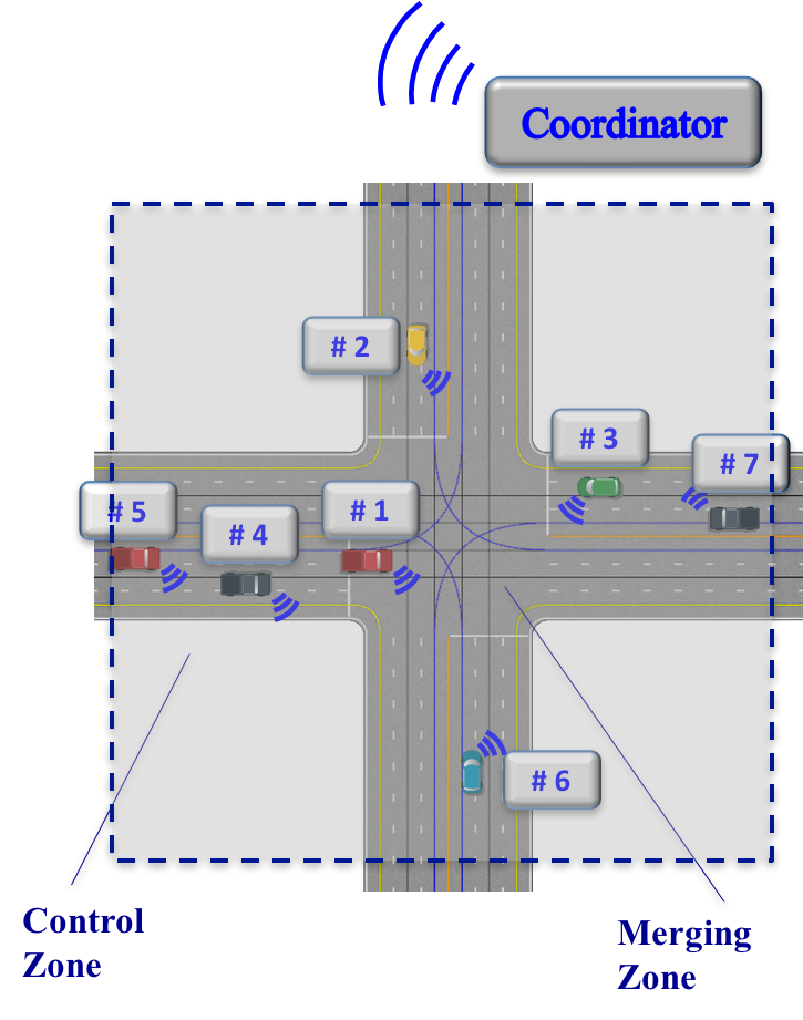
We consider a single urban intersection (Fig. 1). The region at the center of the intersection, called merging zone, is the area of potential lateral collision of the vehicles. The intersection has a control zone and a coordinator that can communicate with the vehicles traveling inside the control zone. Note that the coordinator is not involved in any decision on the vehicle. The distance from the entry of the control zone until the entry of the merging zone is $L$, and it is assumed to be the same for all entry points of the control zone. Note that the $L$ could be in the order of hundreds of $m$ depending on the coordinator’s communication range capability, while $S$ is the length of a typical intersection.

Let $N(t)\in\mathbb{N}$ be the number of CAVs inside the control zone at time $t\in\mathbb{R}^{+}$ and $\mathcal{N}(t)=\{1,\ldots,N(t)\}$ be a queue which designates the order in which these vehicles will be entering the merging zone. Let $t_{i}^{f}$ be the assigned time for vehicle $i$ to exits the control zone. There is a number of ways to assign $t_{i}^{f}$ for each CAV $i$. For example, we may impose a strict first-in-first-out queueing structure, where each vehicle must enter the merging zone in the same order it entered the control zone. The policy through which the “schedule”  is specified is the result of a higher level optimization problem. This policy, which determines the time $t_{i}^{f}$ that each CAV $i$ exits the control zone, can aim at maximizing the throughput at the intersection while ensuring that the lateral collision avoidance constraint never becomes active. Once the desired $t_{i}^{f}$ for each CAV $i$ is determined, it is stored in the coordinator and is not changed. On the other hand, for each CAV $i$, deriving the optimal control input (minimum acceleration/deceleration) to achieve the target $t_{i}^{f}$ can aim at minimizing its fuel consumption [21] while ensuring that the rear-end collision avoidance constraint never becomes active.

Figure 1: An urban intersection with connected and automated vehicles.

In what follows, we assume that a scheme for determining $t_{i}^{f}$ (upon arrival of CAV $i$) is given, and we will focus on a lower level control problem that will yield for each CAV the optimal control input (acceleration/deceleration) to achieve the assigned $t_{i}^{m}$ subject to the state, control, and rear-end collision avoidance constraints.

II-B Vehicle Model and Constraints

We consider a number of CAVs $N(t)\in\mathbb{N}$, where $t\in\mathbb{R}$ is the time, that enter the control zone. We represent the dynamics of each vehicle $i\in\mathcal{N}(t)$, with a state equation

$$\dot{x_{i}}=f(t,x_{i},u_{i}),\qquad x_{i}(t_{i}^{0})=x_{i}^{0},\\$$ (1)

where $t\in\mathbb{R}^{+}$ is the time, $x_{i}(t)$, $u_{i}(t)$ are the state of the vehicle and control input, $t_{i}^{0}$ is the time that vehicle $i$ enters the control zone, and $x_{i}^{0}$ is the value of the initial state. We assume that the dynamics of each vehicle are

$$\begin{split}\dot{p}_{i}&=v_{i}(t)\\ \dot{v}_{i}&=u_{i}(t)\\ \dot{s}_{i}&=\xi_{i}\cdot(v_{k}(t)-v_{i}(t))\end{split}$$ (2)

where $p_{i}(t)\in\mathcal{P}_{i}$, $v_{i}(t)\in\mathcal{V}_{i}$, and $u_{i}(t)\in\mathcal{U}_{i}$ denote the position, speed and acceleration/deceleration (control input) of each vehicle $i$ inside the control zone; $s_{i}(t)\in\mathcal{S}_{i},s_{i}(t)=p_{k}(t)-p_{i}(t)$ denotes the distance of vehicle $i$ from the vehicle $k$ which is physically immediately ahead of $i$, and $\xi_{i}$ is a reaction constant of the vehicle. The sets $\mathcal{P}_{i}$, $\mathcal{V}_{i}$, $\mathcal{U}_{i}$, and $\mathcal{S}_{i}$, $i\in\mathcal{N}(t),$ are complete and totally bounded subsets of $\mathbb{R}$.

Let $x_{i}(t)=\left[p_{i}(t)~{}v_{i}(t)~{}s_{i}(t)\right]^{T}$ denote the state of each vehicle $i$, with initial value $x_{i}^{0}=\left[p_{i}^{0}~{}v_{i}^{0}~{}s_{i}^{0}\right]^{T}$, where $p_{i}^{0}=p_{i}(t_{i}^{0})=0$ at the entry of the control zone, taking values in $\mathcal{X}_{i}=\mathcal{P}_{i}\times\mathcal{V}_{i}$. The state space $\mathcal{X}_{i}$ for each vehicle $i$ is closed with respect to the induced topology on $\mathcal{P}_{i}\times\mathcal{V}_{i}$ and thus, it is compact. We need to ensure that for any initial state $(t_{i}^{0},x_{i}^{0})$ and every admissible control $u(t)$, the system (1) has a unique solution $x(t)$ on some interval $[t_{i}^{0},t_{i}^{f}]$, where $t_{i}^{f}$ is the time that vehicle $i\in\mathcal{N}(t)$ exits the control zone. The following observations from (1) satisfy some regularity conditions required both on $f$ and admissible controls $u(t)$ to guarantee local existence and uniqueness of solutions for (1): a) The function $f$ is continuous in $u$ and continuously differentiable in the state $x$, b) The first derivative of $f$ in $x$, $f_{x}$, is continuous in $u$, and c) The admissible control $u(t)$ is continuous with respect to $t$.

To ensure that the control input and vehicle speed are within a given admissible range, the following constraints are imposed.

$$\begin{split}u_{i,min}&\leq u_{i}(t)\leq u_{i,max},\quad\text{and}\\ 0&\leq v_{min}\leq v_{i}(t)\leq v_{max},\quad\forall t\in[t_{i}^{0},t_{i}^{f}],\end{split}$$ (3)

where $u_{i,min}$, $u_{i,max}$ are the minimum deceleration and maximum acceleration for each vehicle $i\in\mathcal{N}(t)$, and $v_{min}$, $v_{max}$ are the minimum and maximum speed limits respectively.

To ensure the absence of rear-end collision of two consecutive vehicles traveling on the same lane, the position of the preceding vehicle should be greater than or equal to the position of the following vehicle plus a predefined safe distance $\delta_{i}(t)$. Thus we impose the rear-end safety constraint

$$\begin{split}s_{i}(t)=\xi_{i}\cdot(p_{k}(t)-p_{i}(t))\geq\delta_{i}(t),~{}\forall t\in[t_{i}^{0},t_{i}^{f}],\end{split}$$ (4)

where $k$ is some vehicle which is physically immediately ahead of $i$ in the same lane. We relate the minimum safe distance $\delta_{i}(t)$ as a function of speed $v_{i}(t)$,

$$\begin{split}\delta_{i}(t)=\gamma_{i}+\rho_{i}\cdot v_{i}(t),~{}\forall t\in[t_{i}^{0},t_{i}^{f}],\end{split}$$ (5)

where $\gamma_{i}$ is the standstill distance, and $\rho_{i}$ is minimum time gap that vehicle $i$ would maintain while following another vehicle.

Once the time $t_{i}^{f}$ that each vehicle $i\in\mathcal{N}(t)$ will be exiting the control zone is assigned, the problem for each vehicle is to minimize the cost functional $J_{i}(u(t))$, which is the $L^{2}$-norm of the control input in $[t_{i}^{0},t_{i}^{f}]$

$$\min_{u(t)\in U_{i}}J_{i}(u(t))=\frac{1}{2}\int_{t^{0}_{i}}^{t^{f}_{i}}u^{2}_{i}(t)~{}dt,$$ (6)

$$\text{subject to}:\eqref{eq:model2},\eqref{speed_accel constraints},\eqref{eq:rearend},$$

$$\text{and given }t_{i}^{0}\text{, }v_{i}^{0}\text{, }s_{i}(t_{i}^{0})=s_{i}^{0}\text{, }p_{i}(t_{i}^{0})=0\text{, }p_{i}(t_{i}^{f})=L+S,t_{i}^{f}.$$

III Analytical solution of the optimal control problem

Let $\mathbf{S}_{i}(t,x(t))$ be the vector of the constraints in (6) which do not explicitly depend on $u(t)$ [22],

$$\mathbf{S}_{i}\big{(}t,x(t)\big{)}=\begin{bmatrix}v_{i}(t)-v_{max}\\ v_{min}-v_{i}(t)\\ \delta_{i}(t)-s_{i}(t)\end{bmatrix}.$$

Since $\mathbf{S}_{i}(t)\leq\mathbf{0}$ is satisfied for all $t\in[t_{i}^{0},t_{i}^{f}]$, it follows that $\dot{\mathbf{S}}(t)=\leq\mathbf{0}$.

Thus, the Hamiltonian becomes

$$H_{i}\big{(}t,p_{i}(t),v_{i}(t),s_{i}(t),u_{i}(t)\big{)}$$

$$=\frac{1}{2}u(t)^{2}_{i}+\lambda^{p}_{i}\cdot v_{i}(t)+\lambda^{v}_{i}\cdot u_{i}(t)+\lambda^{s}_{i}\cdot\xi_{i}\cdot(v_{k}(t)-v_{i}(t))$$

$$+\mu^{a}_{i}\cdot(u_{i}(t)-u_{max})+\mu^{b}_{i}\cdot(u_{min}-u_{i}(t))$$

$$+\mu^{c}_{i}\cdot u_{i}(t)-\mu^{d}_{i}\cdot u_{i}(t)$$

$$+\mu^{s}_{i}\cdot(\rho_{i}\cdot u_{i}(t)-\xi_{i}\big{(}v_{k}(t)-v_{i}(t)\big{)}),$$ (7)

where $\lambda^{p}_{i}$, $\lambda^{v}_{i}$, and $\lambda^{s}_{i}$ are the influence functions [22], and $\mu^{T}$ is the vector of the Lagrange multipliers.

For each $i\in\mathcal{N}(t)$, the Euler-Lagrange equations are

$$\dot{\lambda}^{p}_{i}(t)=-\frac{\partial H_{i}}{\partial p_{i}}=0,$$ (8)

$$\dot{\lambda}^{v}_{i}(t)=-\frac{\partial H_{i}}{\partial v_{i}}=-(\lambda^{p}_{i}-\lambda^{s}_{i}\cdot\xi_{i}+\mu^{s}_{i}\cdot\xi_{i}),$$ (9)

$$\dot{\lambda}^{s}_{i}(t)=-\frac{\partial H_{i}}{\partial s_{i}}=0,$$ (10)

$$\frac{\partial H_{i}}{\partial u_{i}}=u_{i}(t)+\lambda^{v}_{i}+\mu^{a}_{i}-\mu^{b}_{i}+\mu^{c}_{i}-\mu^{d}_{i}+\mu^{s}_{i}\rho_{i}=0,$$ (11)

with boundary conditions

$$p_{i}(t_{i}^{0})=p_{i}^{0},~{}v_{i}(t_{i}^{0})=v_{i}^{0},~{}s_{i}(t_{i}^{0})=s_{i}^{0},$$

$$p_{i}(t_{i}^{f})=L+S,~{}\lambda^{v}_{i}(t_{i}^{f})=0,~{}\lambda^{s}_{i}(t_{i}^{f})=0,$$ (12)

where $\lambda^{v}_{i}(t_{i}^{f})=\lambda^{s}_{i}(t_{i}^{f})=0$ since the states $v_{i}(t_{i}^{f})$ and $s_{i}(t_{i}^{f})$ are not prescribed at $t_{i}^{f}$ [22].

To address this problem, the constrained and unconstrained arcs will be pieced together to satisfy the Euler-Lagrange equations and necessary condition of optimality. Based on our state and control constraints (3), (4) and boundary conditions, the optimal solution is the result of different combinations of the following possible arcs.

III-1 Inequality State and Control Constraints are not Active

In this case, we have $\mu^{a}_{i}=\mu^{b}_{i}=\mu^{c}_{i}=\mu^{d}_{i}=\mu^{e}_{i}=0.$ Applying the necessary condition (11), the optimal control can be given

$$u_{i}(t)+\lambda^{v}_{i}=0,\quad i\in\mathcal{N}(t).$$ (13)

From (8), (9), and (10) we have $\lambda^{p}_{i}(t)=a_{i}$, $\lambda^{s}_{i}(t)=b_{i}$, and $\lambda^{v}_{i}(t)=-\big{(}(a_{i}-b_{i}\cdot\xi_{i})\cdot t+c_{i}\big{)}$. The coefficients $a_{i}$, $b_{i}$, and $c_{i}$ are constants of integration corresponding to each vehicle $i$. From (13) the optimal control input (acceleration/deceleration) as a function of time is given by

$$u^{*}_{i}(t)=(a_{i}-b_{i}\cdot\xi_{i})\cdot t+c_{i},~{}\forall t\geq t^{0}_{i}.$$ (14)

Substituting the last equation into (2) we find the optimal speed and position for each vehicle, namely

$$v^{*}_{i}(t)=\frac{1}{2}(a_{i}-b_{i}\cdot\xi_{i})\cdot t^{2}+c_{i}\cdot t+d_{i},~{}\forall t\geq t^{0}_{i},$$ (15)

$$p^{*}_{i}(t)=\frac{1}{6}(a_{i}-b_{i}\cdot\xi_{i})\cdot t^{3}+\frac{1}{2}c_{i}\cdot t^{2}+d_{i}\cdot t+e_{i},~{}\forall t\geq t^{0}_{i},$$ (16)

where $d_{i}$ and $e_{i}$ are constants of integration. The constants of integration $a_{i}$, $c_{i}$, $d_{i}$, and $e_{i}$ are computed at each time $t,t^{0}_{i}\leq t\leq t^{f}_{i}$, using the values of the control input, speed, and position of each vehicle $i$ at $t$, the position $p_{i}(t^{f}_{i})$, and the values of the one of terminal transversality condition, i.e., $\lambda^{v}_{i}(t^{f}_{i})$. Since the terminal cost, i.e., the control input, at $t^{f}_{i}$ is zero, we can assign $\lambda^{v}_{i}(t^{f}_{i})=0$.

III-2 The State Constraint $s_{i}(t)=\delta(t)$ Becomes Active

Suppose vehicle $i\in\mathcal{N}(t)$ starts from a feasible state and control at $t=t_{i}^{0}$ and at some time $t=t_{1}\leq t_{i}^{f}$, $s_{i}(t_{1})=\delta(t_{1})$ while $v_{min}<v_{i}(t_{1})<v_{max}$ and $u_{i,min}<u_{i}(t_{1})<u_{i,max}$. In this case, $\mu_{i}^{s}\neq 0$.

Let $N_{i}(t,x(t))=\gamma_{i}+\rho_{i}v_{i}^{*}(t_{1})-\xi_{i}p_{k}^{*}(t_{1})+\xi_{i}p_{i}^{*}(t_{1}).$ Then, we have

$$N_{i}(t,x(t))=\gamma_{i}+\rho_{i}v_{i}^{*}(t_{1})-\xi_{i}(p_{k}^{*}(t_{1})+p_{i}^{*}(t_{1}))=0,$$ (17)

which represents a terminal constraint for the state $s_{i}(t)$ in $t\in[t_{i}^{0},t_{1}].$ Since $N_{i}(t_{1},x(t_{1}))=0$, its first derivative should vanish

$$\dot{N_{i}}(t_{1},x(t_{1}))=\rho_{i}u_{i}^{*}(t_{1})-\xi_{i}(v_{k}^{*}(t_{1})-v_{i}^{*}(t_{1}))=0,$$ (18)

from which we derive the value of the optimal control at $t=t_{1}^{+}$

$$u_{i}^{*}(t_{1}^{+})=\frac{\xi_{i}(v_{k}^{*}(t_{1}^{+})-v_{i}^{*}(t_{1}^{+}))}{\rho_{i}}.$$ (19)

From (14) and (19), we note that the optimal control input is not continuous at $t_{1}$, hence the junction point at $t_{1}$ is a corner. The boundary conditions at the corner for the influence fundtions are

$$\lambda_{i}^{T}(t_{1}^{-})=\lambda_{i}^{T}(t_{1}^{+})+\pi_{i}\frac{\partial{N_{i}(t,x(t))}}{\partial x(t)}.$$ (20)

The transversality condition is

$$\lambda_{i}^{T}(t_{1}^{-})\dot{x}(t_{1}^{-})=\lambda_{i}^{T}(t_{1}^{+})\dot{x}(t_{1}^{+})-\pi_{i}\frac{\partial{N_{i}(t,x(t))}}{\partial t_{1}},$$ (21)

where $\pi_{i}$ is a Lagrange multiplier constant. The influence functions, $\lambda_{i}^{T}(t_{1}^{+})$, at $t_{1}^{+}$, the entry time $t_{1}$, and the Lagrange multipllier $\pi_{i}$ constitute 3+1+1 quantities that are determined so as to satisfy (17), (20), and (21). Note, the values of the influence functions $\lambda_{i}^{T}(t_{1}^{-})$ at $t_{1}^{-}$ are known from the unconstrained arc in $[t_{i}^{0},t_{1}]$, i.e., $\lambda_{i}^{p}(t_{1}^{-})=\alpha_{i}$, $\lambda_{i}^{v}(t_{1}^{-})=-u_{i}^{*}(t_{1}^{-}),$ $\lambda_{i}^{s}(t_{1}^{-})=\beta_{i}$, and the state variables are continuous at the junction point, $t_{1}$, i.e., $p_{i}(t_{1}^{-})=p_{i}(t_{1}^{+}),$ $v_{i}(t_{1}^{-})=v_{i}(t_{1}^{+}),$ $s_{i}(t_{1}^{-})=s_{i}(t_{1}^{+}).$ The unconstrained and constrained arcs are pieced together to determine the 3+1+1 quantities above along with the constants of integration in (14)-(16) while the Hamiltonian at the corner is $H_{i}(t_{1}^{-})=H_{i}(t_{1}^{+})-\pi_{i}\frac{\partial{N_{i}(t,x(t))}}{\partial t_{1}}$.

For the optimal control of the constrained arc, $\delta_{i}(t)-s_{i}(t)\leq 0$, we have the following two cases to consider: (a) when the speed, $v_{k}(t),$ of the preceding vehicle $k$ is decreasing, and (b) when the speed, $v_{k}(t),$ of the preceding vehicle $k$ is either increasing or it is constant.

The speed, $v_{k}(t),$ of the preceding vehicle $k$ is decreasing

Case 1: The exit point $t_{2}$ leads to the arc $u_{i,\min}-u_{i}(t)\leq 0$. Next, we consider the case that the exit point $t_{2}$ of the constrained arc, $\delta_{i}(t)-s_{i}(t)\leq 0,$ leads to the arc $u_{i,\min}-u_{i}(t)\leq 0$. It follows that

$$u_{i}^{*}(t)=u_{i,\min},~{}t\in[t_{2},t_{3}],$$ (22)

where $t_{3}$ is the exit point of the arc $u_{i,\min}-u_{i}(t)\leq 0$. By integrating (22) we have

$$v_{i}^{*}(t) =u_{i,\min}\cdot t+h_{i},~{}t\in[t_{2},t_{3}],$$ (23)

$$p_{i}^{*}(t) =u_{i,\min}\cdot\frac{t^{2}}{2}+h_{i}t+q_{i},~{}t\in[t_{2},t_{3}],$$ (24)

where $h_{i}$ and $q_{i}$ are constants of integration. For the exit point $t_{3}$ of this arc, we have the following result.

If vehicle $i$ remains at the constrained arc, $u_{i,\min}-u_{i}\leq 0$, until $t_{i}^{f}$, then we use the interior constraints and boundary conditions from which we can compute $t_{2}$, and the constants of integrations $h_{i}$ and $q_{i}$. If, however, at some time $t=t_{3}$, vehicle $i$ exits the constrained arc, $u_{i,\min}-u_{i}(t)\leq 0$, and enters the arc $v_{\min}-v_{i}(t)\leq 0$, then it follows that $u_{i}^{*}(t)=0,$ for all $t\in[t_{3},t_{i}^{f}]$, and the optimal speed and position of $i$ are

$$v^{*}_{i}(t) =v_{min},~{}t\in[t_{3},t_{i}^{f}],$$ (25)

$$p^{*}_{i}(t) =v_{min}~{}t+r_{i},~{}t\in[t_{3},t_{i}^{f}],$$ (26)

where $r_{i}$ is a constant of integration. In this case, we piece together the unconstrained with the two constrained arcs, $u_{i,\min}-u_{i}(t)\leq 0$ and $v_{\min}-v_{i}(t)\leq 0$, to satisfy the interior constraints and boundary conditions from which we can compute $t_{2}$, $t_{3}$ and the constants of integration $h_{i},q_{i},$ and $r_{i}$.

Case 2: The exit point $t_{2}$ leads to the arc $v_{\min}-v_{i}(t)\leq 0$. Next, we consider the case that the exit point $t_{2}$ of the constrained arc, $\delta_{i}(t)-s_{i}(t)\leq 0,$ leads to the arc $v_{\min}-v_{i}(t)\leq 0$. It follows that $u_{i}^{*}(t)=0,$ for all $t\in[t_{2},t_{i}^{f}]$, and the optimal speed and position of the vehicle are given by (25) and (26). From the interior constraints and boundary conditions, we can compute $t_{2}$, and the constant of integration $r_{i}$.

The speed, $v_{k}(t),$ of the preceding vehicle $k$ is either increasing or it is constant

The unconstrained arc for all $t\in[t_{2},t_{i}^{f}],$ consists of a set of equations as in (14) - (16) for the optimal control, speed, and position of vehicle $i$, i.e., $u^{*}_{i}(t)=a_{i}^{\prime}\cdot t+c_{i}^{\prime},$ $v^{*}_{i}(t)=\frac{1}{2}a_{i}^{\prime}\cdot t^{2}+c_{i}^{\prime}\cdot t+d_{i}^{\prime},$ and $p^{*}_{i}(t)=\frac{1}{6}a_{i}^{\prime}\cdot t^{3}+\frac{1}{2}c_{i}^{\prime}\cdot t^{2}+d_{i}^{\prime}\cdot t+e_{i}^{\prime},$ where $a_{i}^{\prime},$ $c_{i}^{\prime},$ $d_{i}^{\prime},$ and $e_{i}^{\prime},$ are constants of integration that can be computed along with $t_{2}$ from the interior constraints and boundary conditions.

Similar results are obtained for the remaining cases. To derive the analytical solution of (6), we first start with the unconstrained arc and derive the solution using (14) - (16). If the solution violates any of the state or control constraints, then the unconstrained arc is pieced together with the arc corresponding to the violated constraint, and we re-solve the problem with the two arcs pieced together. The two arcs yield a set of algebraic equations which are solved simultaneously using the boundary conditions of (6) and interior conditions between the arcs. If the resulting solution, which includes the determination of the optimal switching time from one arc to the next one, violates another constraint, then the last two arcs are pieced together with the arc corresponding to the new violated constraint, and we re-solve the problem with the three arcs pieced together. The three arcs will yield a new set of algebraic equations that need to be solved simultaneously using the boundary conditions of (6) and interior conditions between the arcs. The resulting solution includes the optimal switching time from one arc to the next one. The process is repeated until the solution does not violate any other constraints.

IV Simulation Results

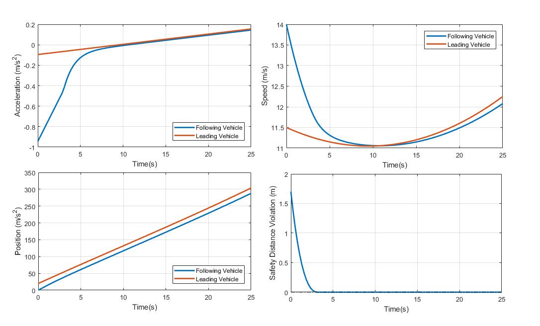
To validate the effectiveness of the analytical solution for real-end collision avoidance, we created a simple driving scenario in MATLAB. The length of the control zone is 300 $m$. The following vehicle $i$ is located at the entry of the control zone (Fig. 1) with the initial speed of 14 $m/s$. At the time that vehicle $i$ enters the control zone, the leading vehicle $k$ has a speed of 11.5 $m/s$ and is located at 20 $m$ (inside the control zone). In this analysis, we set -1 $m/s^{2}$ and 1 $m/s^{2}$ as the minimum and maximum acceleration. For simplification, we set the final time for vehicle $i$ is 26 $s$. We analyzed three cases with different leading vehicle acceleration profiles to test the effectiveness of our model. For comparison, we also include the scenario when the safety constraint is not considered in the optimization model.

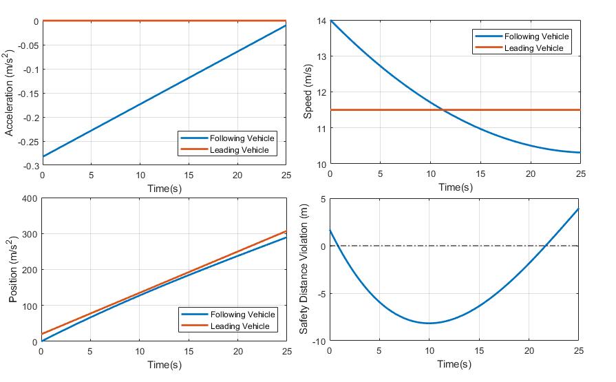
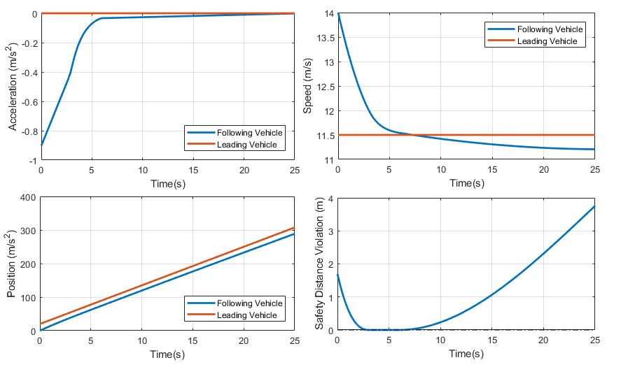
IV-A Case 1: constant acceleration of leading vehicle

In this case, we consider constant speed of leading vehicle $k$. We see that in Fig. 2(a), if the safety constraint is not incorporated in the optimization model, linear acceleration profile is yielded, however, the following distance of vehicle $i$ violates the minimum safety distance. Two vehicles get too close to each other, which creates an extremely unsafe driving situation. Considering the safety constraint, the optimal acceleration profile is presented in Fig. 2(b). We observe three arcs in the optimal acceleration profile, before $t_{1}=3.1$ $s$, the safety constraint is not violated, vehicle $i$ decelerates with a much lower acceleration than the recommended acceleration without safety constraint. At $t_{1}=3.1$ $s$, safety constraint is violated, vehicle $i$ enters the constrained arc at $t_{1}=3.1$ $s$ and leaves constrained arc at $t_{2}=6.5$ $s$.

(a) Results without safety constraint

(b) Results with safety constraint

Figure 2: Optimization results for case 1.

IV-B Case 2: linearly decreasing acceleration of leading vehicle

In this case, we consider a decreasing acceleration profile of vehicle $k$ with a positive initial acceleration. Similar to case 1, the safety constraint is activated. By piecing together the unconstrained and constrained arcs, the results corresponding to the closed form analytical solution are shown in Fig. 3. Before the entry time at $t_{1}=2.9$ $s$, vehicle $i$ travels with a linearly decreasing acceleration until the safety constraint is activated (i.e., $s_{i}(t)-\delta(t)=0$). Since vehicle $i$ keeps decelerating and vehicle $k$ keeps accelerating, vehicle $i$ exits the constraint arc at $t_{2}=5.3$ $s$, when the second unconstrained arc starts.

Figure 3: Optimization results for case 2.

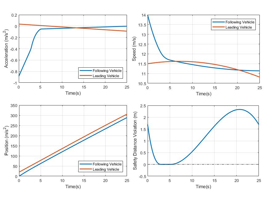
IV-C Case 3: linearly increasing acceleration of leading vehicle

In this case, we consider an increasing acceleration profile of the leading vehicle $k$ with a negative initial acceleration. With the same initial speed setup, vehicle $i$ hits the constrained arc around similar time at $t_{1}=3.0$ $s$. However, since the speed of vehicle $k$ keeps reducing until $t=10.0$ $s$, vehicle $i$ has to decelerate for a longer time to keep the minimum safe distance with vehicle $k$. After $t=10.0$ $s$, vehicle $i$ is not able to leave the constrained arc due to the following reason: vehicle $i$ needs higher acceleration to meet the pre-defined final time, however, the acceleration of vehicle $i$ is limited by the acceleration of vehicle $k$ due to safety constraint. In case 3, we see that vehicle $i$ keeps the minimum safe following distance with vehicle $k$ until the time vehicle $k$ exits the control zone. However, if everything remains unchanged while vehicle $k$ decelerates harder, it is foreseeable that the final time of 26 $s$ is not feasible under current scenario settings.

Figure 4: Optimization results for case 3.

V Concluding Remarks and Discussion

In this paper, we derived a closed-form analytical solution that includes the rear-end safety constraint in addition to the state and control constraints. We augmented the double integrator with an additional state corresponding to the distance of a vehicle from its preceding vehicle. Thus, we included the rear-end collision avoidance constraint as a state constraint while allowing the safe distance between the vehicles to be a function of the vehicle’s speed. The proposed framework is limited to the lower-level individual vehicle operation control, which did not consider the upper-level vehicle coordination problem that designates the sequence that each CAV crosses the merging zone. Ongoing work considers the upper-level problem that results in maximizing the throughput of the intersection and satisfies collision avoidance constraints inside the merging zone. While the potential benefits of full penetration of CAVs to alleviate traffic congestion and reduce fuel consumption have become apparent, different penetrations of CAVs can alter significantly the efficiency of the entire system. Therefore, future research should investigate the implications of different penetration of CAVs.

References

- [1] A. A. Malikopoulos, “A duality framework for stochastic optimal control of complex systems,” IEEE Transactions on Automatic Control, vol. 61, no. 10, pp. 2756–2765, 2016.
- [2] R. Tachet, P. Santi, S. Sobolevsky, L. I. Reyes-Castro, E. Frazzoli, D. Helbing, and C. Ratti, “Revisiting street intersections using slot-based systems,” PLOS ONE, vol. 11, no. 3, 2016.
- [3] K. Dresner and P. Stone, “Multiagent traffic management: a reservation-based intersection control mechanism,” in Proceedings of the Third International Joint Conference on Autonomous Agents and Multiagents Systems, 2004, pp. 530–537.
- [4] K.-D. Kim and P. Kumar, “An MPC-Based Approach to Provable System-Wide Safety and Liveness of Autonomous Ground Traffic,” IEEE Transactions on Automatic Control, vol. 59, no. 12, pp. 3341–3356, 2014.
- [5] A. Colombo and D. Del Vecchio, “Least Restrictive Supervisors for Intersection Collision Avoidance: A Scheduling Approach,” IEEE Transactions on Automatic Control, vol. 60, no. 6, pp. 1515–1527, 2015.
- [6] M. Kamal, M. Mukai, J. Murata, and T. Kawabe, “Model Predictive Control of Vehicles on Urban Roads for Improved Fuel Economy,” IEEE Transactions on Control Systems Technology, vol. 21, no. 3, pp. 831–841, 2013.
- [7] M. Kamal, J. Imura, T. Hayakawa, A. Ohata, and K. Aihara, “A Vehicle-Intersection Coordination Scheme for Smooth Flows of Traffic Without Using Traffic Lights,” IEEE Transactions on Intelligent Transportation Systems, no. 99, 2014.
- [8] G. R. D. Campos, P. Falcone, and J. Sjoberg, “Autonomous Cooperative Driving: a Velocity-Based Negotiation Approach for Intersection Crossing,” in 16th International IEEE Conference on Intelligent Transportation Systems, no. Itsc, 2013, pp. 1456–1461.
- [9] X. Qian, J. Gregoire, A. De La Fortelle, and F. Moutarde, “Decentralized model predictive control for smooth coordination of automated vehicles at intersection,” in 2015 European Control Conference (ECC). IEEE, 2015, pp. 3452–3458.
- [10] G. R. Campos, P. Falcone, H. Wymeersch, R. Hult, and J. Sjoberg, “Cooperative receding horizon conflict resolution at traffic intersections,” in 2014 IEEE 53rd Annual Conference on Decision and Control (CDC), 2014, pp. 2932–2937.
- [11] J. Rios-Torres and A. A. Malikopoulos, “A Survey on Coordination of Connected and Automated Vehicles at Intersections and Merging at Highway On-Ramps,” IEEE Transactions on Intelligent Transportation Systems, vol. 18, no. 5, pp. 1066–1077, 2017.
- [12] A. A. Malikopoulos and L. Zhao, “Decentralized optimal path planning and coordination for connected and automated vehicles at signalized-free intersections,” in 58th IEEE Conference on Decision and Control, 2019.
- [13] J. Rios-Torres, A. A. Malikopoulos, and P. Pisu, “Online Optimal Control of Connected Vehicles for Efficient Traffic Flow at Merging Roads,” in 2015 IEEE 18th International Conference on Intelligent Transportation Systems, 2015, pp. 2432–2437.
- [14] J. Rios-Torres and A. A. Malikopoulos, “Automated and Cooperative Vehicle Merging at Highway On-Ramps,” IEEE Transactions on Intelligent Transportation Systems, vol. 18, no. 4, pp. 780–789, 2017.
- [15] I. A. Ntousakis, I. K. Nikolos, and M. Papageorgiou, “Optimal vehicle trajectory planning in the context of cooperative merging on highways,” Transportation Research Part C: Emerging Technologies, vol. 71, pp. 464–488, 2016.
- [16] Y. Zhang, A. A. Malikopoulos, and C. G. Cassandras, “Optimal control and coordination of connected and automated vehicles at urban traffic intersections,” in Proceedings of the American Control Conference, 2016, pp. 6227–6232.
- [17] L. Zhao, A. A. Malikopoulos, and J. Rios-Torres, “Optimal control of connected and automated vehicles at roundabouts: An investigation in a mixed-traffic environment,” in 15th IFAC Symposium on Control in Transportation Systems, 2018, pp. 73–78.
- [18] A. Stager, L. Bhan, A. A. Malikopoulos, and L. Zhao, “A scaled smart city for experimental validation of connected and automated vehicles,” in 15th IFAC Symposium on Control in Transportation Systems, 2018, pp. 130–135.
- [19] A. A. Malikopoulos, C. G. Cassandras, and Y. Zhang, “A decentralized energy-optimal control framework for connected automated vehicles at signal-free intersections,” Automatica, vol. 93, pp. 244–256, 2018.
- [20] A. A. Malikopoulos, S. Hong, B. Park, J. Lee, and S. Ryu, “Optimal control for speed harmonization of automated vehicles,” IEEE Transactions on Intelligent Transportation Systems, vol. 20, no. 7, pp. 2405–2417, 2019.
- [21] A. A. Malikopoulos, P. Y. Papalambros, and D. N. Assanis, “Online identification and stochastic control for autonomous internal combustion engines,” Journal of Dynamic Systems, Measurement, and Control, vol. 132, no. 2, pp. 024 504–024 504, 2010.
- [22] A. E. Bryson and Y. C. Ho, Applied optimal control: optimization, estimation and control. CRC Press, 1975.