Hill’s equation, tire tracks and rolling cones

Abstract

Louis Poinsot has shown in 1854 that the motion of a rigid body, with one of its points fixed, can be described as the rolling without slipping of one cone, the ‘body cone’, along another, the ‘space cone’, with their common vertex at the fixed point. This description has been further refined by the second author in 1996, relating the geodesic curvatures of the spherical curves formed by intersecting the cones with the unit sphere in Euclidean $\mathbb{R}^{3}$, thus enabling a reconstruction of the motion of the body from knowledge of the space cone together with the (time dependent) magnitude of the angular velocity vector. In this article we show that a similar description exists for a time dependent family of unimodular $2\times 2$ matrices in terms of rolling cones in 3-dimensional Minkowski space $\mathbb{R}^{2,1}$ and the associated ‘pseudo spherical’ curves, in either the hyperbolic plane $H^{2}$ or its Lorentzian analog $H^{1,1}$. In particular, this yields an apparently new geometric interpretation of Schrödinger’s (or Hill’s) equation $\ddot{x}+q(t)x=0$ in terms of rolling without slipping of curves in the hyperbolic plane.

1 Introduction

The motion of a rigid body in $\mathbb{R}^{3}$, with one of its points fixed, consists at every moment of rotation about an instantaneous axis passing through the fixed point, also called the angular velocity axis. This is well known and easy to imagine (see for example the book [1, p. 125]). What is perhaps less well known is the following remarkable 19th century theorem of Louis Poinsot [5], describing the motion in terms of rolling without slipping of one cone along another:

When a body is continuously moving round one of its points, which is fixed, the locus of the instantaneous axis in the body is a cone, whose vertex is at the fixed point: the locus of the instantaneous axis in space is also a cone whose vertex is at the fixed point […] the actual motion of the body can be obtained by making the former of these cones (supposed to be rigidly connected with the body) roll on the latter cone (supposed to be fixed in space). (Quoted from [6, p. 2]). See Figure 1.

Figure 1: Poinsot’s Theorem: the body cone is rolling without slipping on the space cone, and is tangent to it along the instantaneous axis of rotation.

As the second author has shown [4], this rolling cones description can be made more precise: if we intersect each of the cones in Poinsot’s theorem with a sphere centered at the fixed point we obtain a pair of spherical curves whose geodesic curvatures are related by the magnitude of the angular velocity vector ${\bm{\omega}}$, enabling a reconstruction of the motion of the body from knowledge of the space cone together with the (time dependent) magnitude $|{\bm{\omega}}|$ (see Theorem 1 below for the precise statement).

Poinsot’s Theorem can be reformulated more abstractly as a statement about smooth curves in the orthogonal group $\mathrm{SO}_{3}$. It is natural to look for an analog for other groups. In this paper we do that for the Möbius group $\mathrm{PSL}_{2}(\mathbb{R})\simeq\mathrm{SO}_{2,1}$. Poinsot’s Theorem and its refinement of [4] then become a statement about the phase flow of the non-autonomous Hamiltonian linear system of ordinary differential equations

$$\dot{\mathbf{x}}(t)=a(t){\mathbf{x}}(t),$$ (1)

where ${\mathbf{x}}(t)\in\mathbb{R}^{2}$ and $a=a(t)\in\mathfrak{sl}_{2}(\mathbb{R})$, the space of $2\times 2$ traceless matrices. The salient features of this interpretation are:

• Solving equation (1) is equivalent to reconstructing a curve on a ‘pseudo-sphere’ in Minkowski’s space $\mathbb{R}^{2,1}$ from its geodesic curvature.

• The phase flow of (1) can be visualized as a rigid motion in $\mathbb{R}^{2,1}$, under which motion one cone rolls on another without slipping.

• The rigid motion, and thus the solutions to equation(1), is completely determined by two cones, the ‘body cone’ and the ‘space cone’, lying in $\mathbb{R}^{2,1}$ and given explicitly in terms of $a(t)$.

• Unless $a(t)$ is a commuting family of matrices, the system (1) cannot be solved explicitly by the naïve formula ${\mathbf{x}}(t)=\exp\left(\int_{0}^{t}a(\tau)\mathrm{d}\tau\right){\mathbf{x}}(0)$ (unlike in the scalar version of this equation). Nevertheless, the rolling cones interpretation allows for a correction of this formula in terms of parallel transport along curves in the pseudo-sphere in $\mathbb{R}^{2,1}.$ Interestingly, the cumulative angle of rotation appears in the solution despite the fact that the $a(t)$ do not commute.

Plan of the paper. In the next section, Section 2, we describe in more detail Poinsot’s Theorem and its refinement due to [4], see Theorem 1. In Section 3 we formulate our main result, Theorem 2, generalizing Theorem 1 to rigid motions in Minkowski’s space, thus giving a novel ‘rolling cones’ interpretation to the phase flow of system (1). Section 4 contains a proof of both Theorem 1 and 2 in a unified group theoretic language, so as to make the generalization from $\mathrm{SO}_{3}$ to ${\mathrm{SL}_{2}(\mathbb{R})}$ straightforward, see Theorem 3. In the last two sections, we illustrate our main result via two examples of equation (1): periodically perturbed harmonic oscillator (Mathieu’s equation) and the 2D bicycling equation.

2 Background

Consider the motion of a rigid body in Euclidean $\mathbb{R}^{3}$, with one of its points fixed at the origin. If we follow any of the points of the body, initially at ${\mathbf{x}}(0)$, then its position ${\mathbf{x}}(t)\in\mathbb{R}^{3}$ at time $t$ satisfies

$$\dot{\mathbf{x}}(t)={\bm{\omega}}(t)\times{\mathbf{x}}(t),$$

where ${\bm{\omega}}(t)\in\mathbb{R}^{3}$ is the associated angular velocity vector – a vector aligned with the axis of rotation, whose length $|{\bm{\omega}}(t)|$ is the angular velocity of the body about the axis of rotation and whose direction is given by the ‘right hand rule’.

Denote by $a_{\bm{\omega}}:\mathbb{R}^{3}\to\mathbb{R}^{3}$ the map ${\mathbf{x}}\mapsto{\bm{\omega}}\times{\mathbf{x}}$; then the last equation can be rewritten as the non-autonomous linear system

$$\dot{\mathbf{x}}(t)=a(t){\mathbf{x}}(t),\qquad\mbox{where }{\mathbf{x}}(t)\in\mathbb{R}^{3},\ a(t)=a_{{\bm{\omega}}(t)}\in{\mathfrak{so}_{3}},$$ (2)

and where ${\mathfrak{so}_{3}}$ denotes the space of $3\times 3$ antisymmetric real matrices. An equation equivalent to (2) is the equation for its fundamental solution matrix $g(t)\in\mathrm{SO}_{3}$ (the group of $3\times 3$ orthogonal matrices with determinant 1), satisfying

$$\dot{g}(t)=a(t)g(t),\ g(0)=\mathrm{I},\qquad\mbox{ where }\ g(t)\in\mathrm{SO}_{3},\ a(t)=a_{{\bm{\omega}}(t)}\in{\mathfrak{so}_{3}},$$ (3)

and $\mathrm{I}$ denotes the identity $3\times 3$ matrix. The relation between the solutions of equations (2) and (3) is ${\mathbf{x}}(t)=g(t){\mathbf{x}}(0).$

Figure 2 illustrates the above mentioned Poinsot theorem and the geometrical solution of equation (3). In the figure, $\mathscr{C}_{space}$ denotes the locus of rotation axes of the body, the ‘space cone’ (the cone, with vertex at the origin, generated by the space curve ${\bm{\omega}}(t)$). Viewed from a body-fixed frame, the rotation axes form another cone, the ‘body cone’ $\mathscr{C}_{body}$, rigidly attached to the body, with vertex at the origin as well. Then, as the body moves according to equation (3), the cone $\mathscr{C}_{body}$ (rigidly affixed to the body) rolls without slipping along $\mathscr{C}_{space}$: at each moment, $\mathscr{C}_{body}$ is tangent to $\mathscr{C}_{space}$ along the instantaneous axis of rotation, which is (momentarily) at rest.

As shown in [4], this rolling cones description can be made more precise, as follows. For a given non-vanishing ‘space angular velocity’ curve ${\bm{\omega}}(t)$ and a solution $g(t)$ to equation (3), let $\bm{\Omega}(t)=g(t)^{-1}{\bm{\omega}}(t)$ be the ‘body angular velocity’ curve, and $\mathbf{n}(t):={\bm{\omega}}(t)/|{\bm{\omega}}(t)|,\mathbf{N}(t):=\bm{\Omega}(t)/|\bm{\Omega}(t)|$ the (parametrized) intersections of $\mathscr{C}_{space},\mathscr{C}_{body}$ (respectively) with the unit sphere $S^{2}\subset\mathbb{R}^{3}$.

Theorem 1 ([4]).

1. $g(t)$ rolls $\mathbf{N}$ without slipping along $\mathbf{n}$; that is: $g(t)\mathbf{N}(t)=\mathbf{n}(t)$, $g(t)\dot{\mathbf{N}}(t)=\dot{\mathbf{n}}(t)$, for all $t$. See Figure 2.

2. For non vanishing $\dot{\mathbf{n}}$, the (spherical) geodesic curvatures $K,k$ of $\mathbf{N},\mathbf{n}$ (respectively) are related by

   $$K=k-{|{\bm{\omega}}|\over|\dot{\mathbf{n}}|}.$$ (4)

3. Let $R[\Phi(t)]$ be the rotation about ${\bm{\omega}}(0)$ by the angle $\Phi(t)=\int_{0}^{t}|{\bm{\omega}}(\tau)|\mathrm{d}\tau$. Then

   $$g(t)=P_{\mathbf{n}}(t)\circ R[\Phi(t)]\circ P_{\mathbf{N}}(t)^{-1},$$ (5)

   where $P_{\mathbf{N}}(t)$ is (spherical) parallel transport along $\mathbf{N}$ from $\mathbf{N}(0)$ to $\mathbf{N}(t)$, extended to $\mathbb{R}^{3}$ by $\mathbf{N}(0)\mapsto\mathbf{N}(t)$ and similarly for $P_{\mathbf{n}}(t).$

Statement (1) is just a reformulation of Poinsot Theorem. Statement (2), taken together with statement (1), can be thought of as a geometrical/mechanical ‘recipe’ for solving equation (3): given a ‘space angular velocity curve’ ${\bm{\omega}}(t)$, one uses equation (4) to construct $\mathbf{N}(t)$ from its geodesic curvature and the initial conditions $\mathbf{N}(0)=\mathbf{n}(0)$, $\dot{\mathbf{N}}(0)=\dot{\mathbf{n}}(0)$. Then $g(t)\in\mathrm{SO}_{3}$ is the (unique) rigid motion mapping $\mathbf{N}(t)\mapsto\mathbf{n}(t),$ $\dot{\mathbf{N}}(t)\mapsto\dot{\mathbf{n}}(t)$.

Statement (3) of Theorem 1 is a curious fact regarding ‘composition of a non-commuting family of matrices’. Namely, the difficulty of solving (3) explicitly lies in the fact that, in general, the matrices $a(t)$ do not commute for different values of $t$. If, on the other hand, the axis of rotation is fixed, i.e., ${\bm{\omega}}(t)=\omega(t){\mathbf{e}}$ for some fixed unit vector ${\mathbf{e}}$ and a scalar function $\omega(t)$, so that the $a(t)$ commute, then $g(t)$ is the rotation about ${\mathbf{e}}$ by the cumulative angle $\int_{0}^{t}\omega(\tau)\mathrm{d}\tau,$ i.e., $g(t)=\exp\left(\int_{0}^{t}a(\tau)\mathrm{d}\tau\right)$ is the solution to equation (3), just as in the scalar version of equation (3). In spite of the lack of commutativity in general, the cumulative angle still appears in the decomposition formula (5), with an appropriate correction by parallel translations.

Figure 2: A view of the cone $\mathscr{C}_{body}$ rolling along the cone $\mathscr{C}_{space}$ without slipping under the rigid motion $g(t)$. The curves ${\bf N}$, ${\bf n}$ are the intersections of these cones with the unit sphere.

Here is a heuristic explanation for the decomposition formula (5). As the body curve $\mathbf{N}$ rolls along $\mathbf{n}$ in some time range $0\leq t\leq t_{0}$, the vector $\dot{\bf N}(t_{0})$ in Figure 2 swings over and coincides with $\dot{\bf n}(t_{0})$ at $t=t_{0}$. The first key idea is that this hard-to-describe motion can be decomposed into two simpler ones, as shown in Figure 3: tangent transport $T^{-1}_{\bf N}$ of $\dot{\bf N}(t_{0})$ along ${\bf N}$ backwards to ${\bf N}(0)={\bf n}(0)$, followed by tangent transport $T_{\bf n}$ forward along ${\bf n}$ to ${\bf n}(t_{0})$:

$$\dot{\bf n}(t_{0})=(T_{\bf n}\circ T^{-1}_{\bf N})\,\dot{\bf N}(t_{0}).$$ (6)

But

$$T_{\bf n}=P_{\bf n}\circ R(\theta_{\bf n}),\ \ T_{\bf N}=P_{\bf N}\circ R(\theta_{\bf N}),$$

where $P_{\bf n}$ denotes parallel transport along ${\bf n}$, $\theta_{\bf n}$ is the integral of the geodesic curvature of ${\bf n}$ and $R(\theta)$ is the rotation around ${\bf n}(0)={\bf N}(0)$ through the angle $\theta$; thus (6) becomes

$$\dot{\bf n}(t_{0})=g(t_{0})\,\dot{\bf N}(t_{0})=(P_{\bf n}\circ R(\theta_{\bf n}-\theta_{\bf N})\circ P^{-1}_{\bf N})\,\dot{\bf N}(t_{0}).$$ (7)

The second key idea is the observation that the angle $\theta_{\bf n}-\theta_{\bf N}$ turns out to be the time integral of the angular velocity $|{\bm{\omega}}(t)|$ of the rigid motion $g(t)$ – this is made precise by equation (4), relating the geodesic curvatures of ${\bf N}$ and of ${\bf n}$.

Figure 3: The map $\dot{\bf N}(t_{0})\mapsto\dot{\bf n}(t_{0})$ is a composition of tangent transport backwards along ${\bf N}$ and forward along ${\bf n}$. This composition can be accomplished instead by parallel transport backwards along ${\bf N}$, followed by a rotation around the cusp point, followed by parallel transport forward along ${\bf n}$. The angle of the rotation around the cusp turns out to be the integral of the angular velocity of the rigid motions $g(t)\in\mathrm{SO}_{3}$.

3 The main result

We apply the above ideas to gain geometrical insight into the linear system of ordinary differential equations

$$\dot{\mathbf{x}}(t)=a(t){\mathbf{x}}(t),\qquad\mbox{ where }{\mathbf{x}}(t)\in\mathbb{R}^{2},\ a(t)\in\mathfrak{sl}_{2}(\mathbb{R}),$$ (8)

and where $\mathfrak{sl}_{2}(\mathbb{R})$ denotes the set of traceless $2\times 2$ matrices. This system includes, among numerous applications in mathematics, physics and engineering, the 1-dimensional Schrödinger’s, or Hill’s, equation

$$\ddot{x}+q(t)x=0,$$ (9)

where $x=x(t)$ and $q(t)$ are real functions. The last equation is obtained as a special case of (8) by setting

$${\mathbf{x}}(t)={x(t)\choose\dot{x}(t)},\quad a(t)=\left(\begin{matrix}0&1\\ -q(t)&0\end{matrix}\right).$$

Another special case of (8) is the ‘planar bicycle equation’ (see Section 7 below).

The fundamental solution matrix $g$ of (8), defined (as before) by

$$\dot{g}(t)=a(t)g(t),\quad g(0)=\mathrm{I},$$ (10)

lies in ${\mathrm{SL}_{2}(\mathbb{R})}$, the group of $2\times 2$ matrices with determinant 1. As before, the relation between the solutions of equations (8) and (10) is ${\mathbf{x}}(t)=g(t){\mathbf{x}}(0).$

The starting point of our approach is the observation that the linear area–preserving flow in $\mathbb{R}^{2}$ of equation (8) can equivalently be viewed as a rigid motion in the Lie algebra $\mathfrak{sl}_{2}(\mathbb{R})$. More precisely, instead of considering the motion of points in $\mathbb{R}^{2}$ under $g\in{\mathrm{SL}_{2}(\mathbb{R})}$, we consider the motion of points in $\mathfrak{sl}_{2}(\mathbb{R})$, the $3$–dimensional Lie algebra of ${\mathrm{SL}_{2}(\mathbb{R})}$, given by conjugation with $g$:

$${\rm Ad}_{g}:\mathfrak{sl}_{2}(\mathbb{R})\rightarrow\mathfrak{sl}_{2}(\mathbb{R}),\quad a\mapsto gag^{-1},\quad a\in\mathfrak{sl}_{2}(\mathbb{R}),\quad g\in{\mathrm{SL}_{2}(\mathbb{R})}.$$

Now ${\rm Ad}_{g}$, being a conjugation, preserves the spectrum of each $a\in\mathfrak{sl}_{2}(\mathbb{R})$, and in particular, $\det(a)$. Since $\mbox{tr}(a)=0$, $\det(a)$ turns out to be an indefinite quadratic form, which makes $\mathfrak{sl}_{2}(\mathbb{R})$ a Minkowski space (we provide the details later in Section 4.1). Thus, ${\rm Ad}_{g}$ is an orthogonal transformation of the Minkowski space $\mathfrak{sl}_{2}(\mathbb{R})\simeq\mathbb{R}^{2,1}$, a ‘rigid motion’. The map $g\mapsto{\rm Ad}_{g}$ is $2$ to $1$, so up to a minor ambiguity, all properties of $g$ can be recovered from those of ${\rm Ad}_{g}$. For instance, $g$ is elliptic, i.e., conjugate to a rotation of $\mathbb{R}^{2}$ through an angle $\theta$, if and only if ${\rm Ad}_{g}$ is a rigid rotation in $\mathfrak{sl}_{2}(\mathbb{R})$ (in the Minkowski metric) around a timelike axis, rotating the orthogonal (spacelike) plane through the angle $2\theta$; similar statements hold for parabolic and hyperbolic elements in ${\mathrm{SL}_{2}(\mathbb{R})}$.

One advantage of looking at ${\rm Ad}_{g}$ acting on $\mathfrak{sl}_{2}(\mathbb{R})$ (versus $g$ acting on $\mathbb{R}^{2}$) is that a geometry (hidden heretofore in $\mathbb{R}^{2}$) is revealed; the already mentioned orthogonality of ${\rm Ad}_{g}$ is one example. Furthermore, orthogonal transformations of Minkowski’s space, just like Euclidean ones, have axes of rotation: lightlike for the elliptic rotations and spacelike for the hyperbolic ones; in $\mathbb{R}^{2}$, none of this is visible.

By carrying through this analogy between Euclidean and Minkowski rigid motions, we then obtain, with some minor modifications due to sign and nullity details, the following almost-verbatim Minkowski version of Theorem 1.

Theorem 2.

Let $a(t)\in\mathfrak{sl}_{2}(\mathbb{R})$ be a given non-vanishing ‘space angular velocity’ curve with non vanishing $|a|:=2\sqrt{|\det(a)|}$ and let $g(t)\in{\mathrm{SL}_{2}(\mathbb{R})}$ be the solution to $\dot{g}=ag,$ $g(0)=\mathrm{I}$. Let $A=g^{-1}ag$ be the associated ‘body angular velocity’ curve and $\mathbf{n}:=a/|a|,\mathbf{N}:=A/|A|$ be the projections of $a,A$ (respectively) on the unit ‘pseudo-sphere’ $\Sigma\subset\mathfrak{sl}_{2}(\mathbb{R})$ (either the hyperbolic plane $H^{2}$ or its Lorentzian analog $H^{1,1}$, depending on the sign of $\det(a)$; see Section 4.1 below for details). Then

1. $g(t)$ rolls $\mathbf{N}$ without slipping along $\mathbf{n}$, i.e., ${\rm Ad}_{g(t)}\mathbf{N}(t)=\mathbf{n}(t)$, ${\rm Ad}_{g(t)}\dot{\mathbf{N}}(t)=\dot{\mathbf{n}}(t)$, for all $t$.

2. For non vanishing $|\dot{\mathbf{n}}|$, the (pseudo-spherical) geodesic curvatures $K,k$ of $\mathbf{N},\mathbf{n}$ (respectively) are related by

   $$K=k-{|{\bm{\omega}}|\over|\dot{\mathbf{n}}|}.$$

3. Let $R[\Phi(t)]$ be the (pseudo) rotation about $a(0)$ by the angle $\Phi(t)=\int_{0}^{t}|{\bm{\omega}}(\tau)|\mathrm{d}\tau$. Then

   $${\rm Ad}_{g(t)}=P_{\mathbf{n}}(t)\circ R[\Phi(t)]\circ P_{\mathbf{N}}(t)^{-1},$$

   where $P_{\mathbf{N}}(t)$ is parallel transport along $\mathbf{N}$ from $\mathbf{N}(0)$ to $\mathbf{N}(t)$, extended to $\mathfrak{sl}_{2}(\mathbb{R})$ by $\mathbf{N}(0)\mapsto\mathbf{N}(t)$ and similarly for $P_{\mathbf{n}}(t).$

Remark 3.1.

In the above theorem, the assumption that $|a(t)|$ is non-vanishing, i.e., the space angular velocity is nowhere null, is essential. For the special case of Hill’s equation (9), this amounts to assuming that the potential $q(t)$ does not vanish for all $t$. Studying this case of $a$ crossing the null cone remains an interesting question which we do not address in this paper.

4 Notation and setup

We start with a review of some notation and terminology, mostly standard.

4.1 Geometry and algebra of $\mathrm{SO}_{3}$ and ${\mathrm{SL}_{2}(\mathbb{R})}$

Denote in the following by $G$ either $\mathrm{SO}_{3}$ or ${\mathrm{SL}_{2}(\mathbb{R})}$ and by $\mathfrak{g}$ its Lie algebra, either $\mathfrak{so}_{3}$ or $\mathfrak{sl}_{2}(\mathbb{R})$, respectively. The conjugation action of $G$ on $\mathfrak{g}$, ${\rm Ad}:G\to\mathrm{GL}(\mathfrak{g}),$ is denoted by

$${\rm Ad}_{g}(a)=g\cdot a:=gag^{-1},\quad g\in G,\ a\in\mathfrak{g}.$$ (11)

Define an Ad-invariant inner product on $\mathfrak{g}$ by

$$\langle a,b\rangle:=\lambda\,\mbox{tr}(ab),\mbox{ where $\lambda=-{1\over 2}$ for $\mathfrak{g}=\mathfrak{so}_{3}$ and $\lambda=2$ for $\mathfrak{g}=\mathfrak{sl}_{2}(\mathbb{R}).$}$$ (12)

Our choice of the normalization factor for each $\mathfrak{g}$ will be explained in a moment. In either case, we set

$$|a|:=\sqrt{|\langle a,a\rangle|}.$$

The ${\rm Ad}$-invariance of $\langle\ ,\ \rangle$ implies that $b\mapsto[a,b]=ab-ba$ is an anti symmetric operator on $\mathfrak{g}$ with respect to $\langle\ ,\ \rangle$, i.e., $\langle[a,b],c\rangle=-\langle b,[a,c]\rangle$ for all $a,b,c\in\mathfrak{g}$, hence

$$\langle[a,b],a\rangle=0,\quad\forall a,b\in\mathfrak{g}.$$ (13)

Let us examine the resulting geometry of $\mathfrak{g}$ in each of the two cases.

Case 1: $\mathfrak{g}=\mathfrak{so}_{3}$. With the choice $\lambda=-{1\over 2}$ in (12), $\langle a,b\rangle:=-\mbox{tr}(ab)/2$ is a positive definite inner product on $\mathfrak{so}_{3}$, the image of the standard inner product on $\mathbb{R}^{3}$ under the isomorphism $\mathbb{R}^{3}\to{\mathfrak{so}_{3}}$, $\bm{\omega}\mapsto a_{{\bm{\omega}}}\in\mathfrak{so}_{3}$, where $a_{{\bm{\omega}}}{\mathbf{x}}:={\bm{\omega}}\times{\mathbf{x}}.$ Explicitly,

$${\bm{\omega}}=\left(\begin{array}[]{c}\omega_{1}\\ \omega_{2}\\ \omega_{3}\end{array}\right)\mapsto a_{{\bm{\omega}}}=\left(\begin{array}[]{ccc}0&-\omega_{3}&\omega_{2}\\ \omega_{3}&0&-\omega_{1}\\ -\omega_{2}&\omega_{1}&0\end{array}\right).$$ (14)

Furthermore, under this isomorphism, the cross product ${\bf u}\times\mathbf{v}$ corresponds to the Lie bracket $[a,b]=ab-ba$ and the standard action of $\mathrm{SO}_{3}$ on $\mathbb{R}^{3}$ corresponds to the conjugation action (11); that is,

$$\langle a_{\bf u},a_{\mathbf{v}}\rangle={\bf u}\cdot\mathbf{v},\ [a_{\bf u},a_{\mathbf{v}}]=a_{{\bf u}\times\mathbf{v}},\ g\cdot a_{\bf u}=a_{g{\bf u}},\quad\mbox{for }g\in\mathrm{SO}_{3},\ {\bf u},\mathbf{v}\in\mathbb{R}^{3}.$$

Case 2: $\mathfrak{g}=\mathfrak{sl}_{2}(\mathbb{R})$. The Lie algebra $\mathfrak{sl}_{2}(\mathbb{R})$ consists of traceless $2\times 2$ real matrices, which we choose to write in the form

$$a={1\over 2}\left(\begin{matrix}a_{1}&a_{2}+a_{3}\\ a_{2}-a_{3}&-a_{1}\end{matrix}\right),$$

so that $\langle a,b\rangle:=2\mbox{tr}(ab)=a_{1}b_{1}+a_{2}b_{2}-a_{3}b_{3}.$ Thus the inner product is indefinite, of signature $++-$ (the ‘spacelike sign convention’). A simpler formula for the associated quadratic form is

$$\langle a,a\rangle=(a_{1})^{2}+(a_{2})^{2}-(a_{3})^{2}=-4\det(a),\quad a\in\mathfrak{sl}_{2}(\mathbb{R}).$$

An element $a\in\mathfrak{sl}_{2}(\mathbb{R})$ is called timelike if $\langle a,a\rangle<0,$ lightlike (or null) if $\langle a,a\rangle=0$ and spacelike if $\langle a,a\rangle>0.$ These are the three causal types of elements in $\mathfrak{sl}_{2}(\mathbb{R})$, also referred to as elliptic, parabolic and hyperbolic, respectively.

The reason for our choice $\lambda=2$ in formula (12) for $\mathfrak{g}=\mathfrak{sl}_{2}(\mathbb{R})$ is the following analog of a familiar property of the vector product in $\mathbb{R}^{3}$.

Lemma 4.1.

If $a,b\in\mathfrak{sl}_{2}(\mathbb{R})$ is an orthonormal pair, i.e., $|a|=|b|=1$ and $\langle a,b\rangle=0$, then $(a,b,[a,b])$ is an orthonormal frame in $\mathfrak{sl}_{2}(\mathbb{R})$, positively oriented with respect to the standard volume form $a_{1}\wedge a_{2}\wedge a_{3}$ if $a,b$ are spacelike, and negatively oriented if one of them is timelike.

Proof.

It is easy to check that

$${\bf i}:=\frac{1}{2}\left(\begin{array}[]{cc}1&0\\ 0&-1\end{array}\right),\quad{\bf j}:=\frac{1}{2}\left(\begin{array}[]{cc}0&1\\ 1&0\end{array}\right),\quad{\bf k}:=\frac{1}{2}\left(\begin{array}[]{cc}0&1\\ -1&0\end{array}\right)$$ (15)

is an orthonormal basis of $\mathfrak{sl}_{2}(\mathbb{R})$, dual to $a_{1},a_{2},a_{3}$, hence it is positively oriented with respect to $a_{1}\wedge a_{2}\wedge a_{3}.$ Furthermore, $\mathbf{i},\mathbf{j}$ are spacelike and $\mathbf{k}$ is timelike, satisfying

$$[{\bf i},{\bf j}]={\bf k},\ \ [{\bf j},{\bf k}]=-{\bf i},\ \ [{\bf k},{\bf i}]=-{\bf j}.$$ (16)

Now let $a,b\in\mathfrak{sl}_{2}(\mathbb{R})$ be an orthonormal pair. Since $a,b$ are not null and orthogonal, both are spacelike or one is timelike and the other spacelike. In the first case, where $a,b$ are spacelike orthogonal unit vectors, by conjugating by an appropriate element of ${\mathrm{SL}_{2}(\mathbb{R})}$ and (possibly) permuting them (neither operation changes the orientation of $(a,b,[a,b])$), we can assume that $a=\mathbf{i}$, $b=\mathbf{j}$, thus $[a,b]=\mathbf{k}$, hence $(a,b,[a,b])$ is a positively oriented orthonormal frame.

In the second case, where one of $a,b$ is timelike and the other spacelike, by (possibly) permuting $a$ and $b$ and changing $a$ to $-a$ (these operations do not affect the orientation of $(a,b,[a,b])$), we can assume that $a$ is timelike future pointing ($a_{3}>0$) and $b$ is spacelike. Next, by conjugating by an appropriate element of ${\mathrm{SL}_{2}(\mathbb{R})}$, we can assume that $a=\mathbf{k}$ and $b=\mathbf{i}$, so that $[a,b]=-\mathbf{j}$, and hence $(a,b,[a,b])$ is a negatively oriented orthonormal frame, as claimed. ∎

Remark 4.2.

The commutation relations (16) differ from the analogous relations for the cross product in $\mathbb{R}^{3}$ by the “$-$” sign when the timelike vector ${\bf k}$ occurs in the commutator. Putting it differently, when taking the cross product in the Minkowski space $\mathfrak{sl}_{2}(\mathbb{R})$, one uses the ‘right-hand rule’ to determine the direction of the cross product of two spacelike vectors, and the ‘left-hand rule’ whenever a timelike vector participates in the cross product.

4.2 Rolling without slipping

Denote by $\Sigma\subset\mathfrak{g}$ the unit (pseudo) sphere, i.e., the set of elements $a\in\mathfrak{g}$ with $\langle a,a\rangle=\pm 1.$ Thus, for $\mathfrak{g}=\mathfrak{so}_{3}$, $\Sigma$ is the standard 2-sphere $S^{2}=\{a\in\mathfrak{so}_{3}\,|\,\langle a,a\rangle=1\}$, while for $\mathfrak{g}=\mathfrak{sl}_{2}(\mathbb{R})$, $\Sigma$ is either $H^{2}:=\{a\in\mathfrak{sl}_{2}(\mathbb{R})\,|\,\langle a,a\rangle=-1\}$ (hyperboloid of two sheets), or $H^{1,1}:=\{a\in\mathfrak{sl}_{2}(\mathbb{R})\,|\,\langle a,a\rangle=1\}$ (hyperboloid of one sheet), see Figure 4.

Figure 4: Level sets of $\langle a,a\rangle=(a_{1})^{2}+(a_{2})^{2}-(a_{3})^{2}$ in $\mathfrak{sl}_{2}(\mathbb{R})$.

Now let $g(t)$ be a smoothly parametrized curve in $G$ with $g(0)=\mathrm{I}$ (the identity element in $G$). Define

$$A(t):=g^{-1}(t)\,\dot{g}(t),\quad a(t):=\dot{g}(t)\,g^{-1}(t)\in\mathfrak{g},$$ (17)

the body and space angular velocities, respectively, and

$$\mathbf{N}(t):=A(t)/|A(t)|,\quad\mathbf{n}(t):=a(t)/|a(t)|,$$ (18)

the radial projections of $A(t),a(t)$ (respectively) onto $\Sigma\subset\mathfrak{g}$. Note that in order to define the (pseudo) spherical curves $\mathbf{N}(t),\mathbf{n}(t),$ we need to assume that $|a(t)|\neq 0$ for all $t$, which we assume henceforth. For $G=\mathrm{SO}_{3}$ this amounts to $a(t)\neq 0$; for $G={\mathrm{SL}_{2}(\mathbb{R})}$ it means that $a(t)$ is non null for all $t$, i.e., it is either spacelike or timelike.

From equations (11) and (17), we have

$$\dot{g}=ag=gA,\ a=g\cdot A,\ \mathbf{n}=g\cdot\mathbf{N},\ g(0)=\mathrm{I}.$$ (19)

Remark 4.3 (About notation).

Sometimes, as in (19), we suppress the explicit dependence on $t$, i.e., $g=g(t),$ $a=a(t)$, etc.

Definition 4.4 (Rolling without slipping).

Let $\Gamma(t),\gamma(t)$ be two parametrized curves in $\mathfrak{g}$. A rolling without slipping of $\Gamma$ along $\gamma$ is a parametrized curve $g(t)$ in $G$, satisfying for all $t$ the contact and no slip conditions:

$$g(t)\cdot\Gamma(t) =\gamma(t),$$ (20)

$$g(t)\cdot\dot{\Gamma}(t) =\dot{\gamma}(t).$$ (21)

See Figure 5.

Figure 5: Rolling of a curve $\Gamma$ along $\gamma$ via a family of isometries ${\rm Ad}_{g(t)}.$

Lemma 4.5.

The no-slip condition (21) is equivalent to

$$[a,\gamma]=0,$$ (22)

where $a=\dot{g}g^{-1}.$ This expresses the vanishing of the velocity of the ‘material point’ of the moving curve at the contact point $g(t)\cdot\Gamma(t)$ between the two curves.

Proof.

Taking the derivative with respect to $t$ of equation (20) and using equations (19),

$$[a,\gamma]+g\cdot\dot{\Gamma}=\dot{\gamma}.$$

Thus $g\cdot\dot{\Gamma}=\dot{\gamma}$ (equation (21)) is equivalent to $[a,\gamma]=0$. ∎

4.3 Geodesic curvature

Let $\gamma(t)$ be a smoothly parametrized (pseudo) spherical curve in $\Sigma\subset\mathfrak{g}$ with nowhere null tangent, i.e., $|\dot{\gamma}|$ does not vanish, and let $\gamma^{\prime}:=\dot{\gamma}/|\dot{\gamma}|$ be the unit tangent along $\gamma$. Then $(\gamma,\gamma^{\prime},[\gamma,\gamma^{\prime}])$ is a ‘moving’ orthonormal frame along $\gamma$.

Notation. We denote henceforth by dot derivative along a curve $\gamma$ with respect to an arbitrary parameter $t$, $\dot{\gamma}:=\mathrm{d}\gamma/\mathrm{d}t,$ and by prime derivative with respect to arc length parameter $s$, $\gamma^{\prime}:=\mathrm{d}\gamma/\mathrm{d}s=\dot{\gamma}/|\dot{\gamma}|$ (provided $|\dot{\gamma}|$ does not vanish).

Definition 4.6.

The geodesic curvature of an oriented (pseudo) spherical curve $\gamma$ in $\Sigma\subset\mathfrak{g}$ with nowhere null tangent is its normal acceleration, i.e., the coefficient of $[\gamma,\gamma^{\prime}]$ in the decomposition of $\gamma^{\prime\prime}$ as a linear combination of $\gamma,\gamma^{\prime},[\gamma,\gamma^{\prime}]$.

This definition can be also expressed conveniently as

$$\gamma^{\prime\prime}\equiv k[\gamma,\gamma^{\prime}]\ {\rm mod\;}\gamma,\gamma^{\prime}.$$ (23)

For an arbitrary parametrization $\gamma(t)$, $\gamma^{\prime\prime}\equiv\ddot{\gamma}/|\dot{\gamma}|^{2}\equiv k[\gamma,\gamma^{\prime}]\ {\rm mod\;}\gamma,\gamma^{\prime}$, from which follows

$$\ddot{\gamma}\equiv k|\dot{\gamma}|[\gamma,\dot{\gamma}]\ \ {\rm mod\;}\gamma,\dot{\gamma}.$$

Remark 4.7 (About the sign of the geodesic curvature).

Our Definition 4.6 of geodesic curvature may differ in sign from other common definitions in the literature, since this sign depends on the choice of a unit normal to the curve. Our choice of unit normal $[\gamma,\gamma^{\prime}]$ is mostly for simplicity in subsequent formulas. At any rate, all applications of this definition in this article are invariant under sign change of $k$. For example, equation (26) below.

4.4 Parallel transport

A vector field $v(t)$ tangent to $\Sigma$ along $\gamma(t)$ is parallel if $\dot{v}(t)\perp T_{\gamma(t)}\Sigma$ for all $t$. That is,

$$\dot{v}\equiv 0\quad{\rm mod\;}\gamma.$$

Any initial vector $v(0)\in T_{\gamma(0)}\Sigma$ can be extended uniquely to parallel vector field $v(t)$ along $\gamma$, by solving the last displayed equation (a linear system of ODEs). The resulting map $P_{\gamma}(t):T_{\gamma(0)}\Sigma\to T_{\gamma(t)}\Sigma$, $v(0)\mapsto v(t)$, is an isometry (with respect to the restriction of $\langle\ ,\ \rangle$ to $\Sigma$), called parallel transport along $\gamma$.

The two notions, geodesic curvature and parallel transport, are related as follows. Let $\gamma(t)$ be a (pseudo) spherical curve with non vanishing $|\dot{\gamma}|$ and $v(t)$ the parallel transport of $\gamma^{\prime}(0)$ along $\gamma$ (or any parallel vector field along $\gamma$ with the same causal type as $\gamma^{\prime}$). At each point $\gamma(t)$ along the curve, $\gamma^{\prime}$ is related to $v$ by a unique orientation preserving isometry $R(\theta)$ of $T_{\gamma(t)}\Sigma$, with ‘rotation angle’ $\theta$. That is, in the Riemannian case,

$$\gamma^{\prime}=R(\theta)v=(\cos\theta)v+(\sin\theta)[\gamma,v],\quad\Sigma=S^{2}\mbox{ or }H^{2},$$ (24)

and in the Lorentzian case

$$\gamma^{\prime}=R(\theta)v=(\cosh\theta)v+(\sinh\theta)[\gamma,v],\quad\Sigma=H^{1,1}.$$ (25)

Lemma 4.8.

For any oriented curve $\gamma$ in $\Sigma$ with non-null tangent, its geodesic curvature is the rate of change, with respect to arc length, of the ‘rotation angle’ of the unit tangent $\gamma^{\prime}$, relative to a parallel unit vector of the same causal type as $\gamma^{\prime}$, as defined in equations (24)-(25); that is,

$$k=\theta^{\prime}.$$

It follows that

$$\gamma^{\prime}(t)=R\left[\theta(t)\right]P_{\gamma}(t)\gamma^{\prime}(0)=P_{\gamma}(t)R\left[\theta(t)\right]\gamma^{\prime}(0),$$

where

$$\theta(t)=\int_{0}^{L_{t}}k\,\mathrm{d}s=\int_{0}^{t}k|\dot{\gamma}|\mathrm{d}\tau,$$

and where $s$ is an arc length parameter along $\gamma$, $L_{t}$ is the length of $\gamma$ between $\gamma(0)$ and $\gamma(t)$ and $\tau$ is the same parameter as $t$.

Proof.

From $\gamma^{\prime}=R(\theta)v$ follows, by a simple calculation, $\gamma^{\prime\prime}=\theta^{\prime}(\partial_{\theta}R(\theta))v+R(\theta)v^{\prime}\equiv\theta^{\prime}[\gamma,R(\theta)v]=\theta^{\prime}[\gamma,\gamma^{\prime}]\ {\rm mod\;}\gamma$, implying $k=\theta^{\prime}$. ∎

Remark 4.9.

In case $\Sigma=H^{1,1}$, $|\dot{\gamma}(t_{0})|$ may vanish even if $\dot{\gamma}(t_{0})\neq 0.$ Then one cannot reparametrize $\gamma$ by arc length and $k$ becomes infinite at $t=t_{0}$. It would be interesting to understand the significance of this phenomena for a linear system $\dot{g}=ag$.

5 The combined theorem and its proof

With the above background we now state and prove the following result, which combines Theorems 1 and 2.

Theorem 3.

Let $G$ be either ${\mathrm{SL}_{2}(\mathbb{R})}$ or $\mathrm{SO}_{3}$, $\mathfrak{g}$ its Lie algebra, $a(t)$ a smoothly parametrized curve in $\mathfrak{g}$ with non-vanishing $|\dot{a}|$, and $g(t)\in G$ the solution to $\dot{g}=ag$, $g(0)=\mathrm{I}$. Set $A(t)=g^{-1}(t)a(t),$ and $\mathbf{N}(t),\mathbf{n}(t)$ the corresponding normalized (pseudo) spherical curves in $\Sigma\subset\mathfrak{g}$, as defined in equations (17)–(18). Then

1. (Poinsot Theorem) $g(t)$ rolls without slipping the curve $A(t)$ along $a(t)$ and $\mathbf{N}(t)$ along $\mathbf{n}(t)$.

2. (The reconstruction formula) If $|\dot{\mathbf{n}}|$ is non-vanishing then the geodesic curvatures $K,k$ of the (pseudo) spherical curves $\mathbf{N},\mathbf{n}$ (respectively) are related by

   $$K=k-{|a|\over|\dot{\mathbf{n}}|}.$$ (26)

3. (The decomposition formula)

   $${\rm Ad}_{g(t)}=\tilde{P}_{\mathbf{n}}(t)\circ R\left[\Phi(t)\right]\circ(\tilde{P}_{\mathbf{N}}(t))^{-1},$$

   where $\tilde{P}_{\mathbf{n}}(t)$ is parallel transport $T_{\mathbf{n}(0)}\Sigma\to T_{\mathbf{n}(t)}\Sigma$ along $\mathbf{n}$, extended to $\mathfrak{g}$ by $\mathbf{n}(0)\mapsto\mathbf{n}(t)$, similarly for $\tilde{P}_{\mathbf{N}}(t)$, and $R\left[\Phi(t)\right]$ is the (pseudo) rotation around the axis $a(0)$ by the angle $\Phi(t)=\int_{0}^{t}|a(\tau)|\mathrm{d}\tau.$

Proof.

(1) If $\gamma=g\cdot\Gamma$ then $\dot{\gamma}=\dot{g}\cdot\Gamma+g\cdot\dot{\Gamma}=[a,\gamma]+g\cdot\dot{\Gamma}.$ For $\gamma=a,\Gamma=A$, since $a=g\cdot A$ and $[a,a]=0$, we get $\dot{a}=g\cdot\dot{A}.$ Next, $\mathbf{n}=g\cdot\mathbf{N}$ implies $\dot{\mathbf{n}}=[a,\mathbf{n}]+g\cdot\dot{\mathbf{N}}=|a|^{-1}[a,a]+g\cdot\dot{\mathbf{N}}=g\cdot\dot{\mathbf{N}}$.

(2) Applying $g$ to $\ddot{\mathbf{N}}\equiv K|\dot{\mathbf{N}}|[\mathbf{N},\dot{\mathbf{N}}]\ ({\rm mod\;}\mathbf{N},\dot{\mathbf{N}})$, we obtain $g\cdot\ddot{\mathbf{N}}\equiv K|\dot{\mathbf{n}}|[\mathbf{n},\dot{\mathbf{n}}]\ ({\rm mod\;}\mathbf{n},\dot{\mathbf{n}}).$ Taking derivative of $\dot{\mathbf{n}}=g\cdot\dot{\mathbf{N}}$, we get $\ddot{\mathbf{n}}=[a,\dot{\mathbf{n}}]+g\cdot\ddot{\mathbf{N}}=|a|[\mathbf{n},\dot{\mathbf{n}}]+g\cdot\ddot{\mathbf{N}}\equiv(|a|+K|\dot{\mathbf{n}}|)[\mathbf{n},\dot{\mathbf{n}}]\ ({\rm mod\;}\mathbf{n},\dot{\mathbf{n}}).$ On the other hand, $\ddot{\mathbf{n}}\equiv k|\dot{\mathbf{n}}|[\mathbf{n},\dot{\mathbf{n}}]\ ({\rm mod\;}\mathbf{n},\dot{\mathbf{n}}),$ hence $|a|+K|\dot{\mathbf{n}}|=k|\dot{\mathbf{n}}|,$ which gives formula (26).

(3) Both sides of the equation are orientation preserving isometries of $\mathfrak{g}$, mapping $\mathbf{N}(t)\mapsto\mathbf{n}(t)$, hence it is enough to show that they coincide on $\mathbf{N}^{\prime}(t)$. By Lemma 4.8 and equation (26),

$$\mathbf{n}^{\prime}(t)=P_{\mathbf{n}}(t)R\left[\theta(t)\right]\mathbf{n}^{\prime}(0),\qquad\mathbf{N}^{\prime}(t)=P_{\mathbf{N}}(t)R\left[\Theta(t)\right]\mathbf{N}^{\prime}(0),$$

where $\theta(t)=\int_{0}^{L_{t}}k\,\mathrm{d}s$ and

$$\Theta(t)=\int_{0}^{L_{t}}K\,\mathrm{d}s=\int_{0}^{L_{t}}\left(k-{|a|\over|\dot{\mathbf{n}}|}\right)\mathrm{d}s=\int_{0}^{L_{t}}k\,\mathrm{d}s-\int_{0}^{t}|a|\mathrm{d}\tau=\theta(t)-\Phi(t).$$

It follows that

$$P_{\mathbf{n}}(t)R\left[\Phi(t)\right](P_{\mathbf{N}}(t))^{-1}\mathbf{N}^{\prime}(t) =P_{\mathbf{n}}(t)R\left[\Phi(t)\right]R\left[\theta(t)\right]\mathbf{N}^{\prime}(0)=$$

$$=P_{\mathbf{n}}(t)R\left[\Phi(t)+\Theta(t)\right]\mathbf{N}^{\prime}(0)=$$

$$=P_{\mathbf{n}}(t)R\left[\theta(t)\right]\mathbf{n}^{\prime}(0)=\mathbf{n}^{\prime}(t),$$

as claimed. ∎

6 Example: the Mathieu equation (timelike angular velocity)

In this section we illustrate Theorem 3 for $G={\mathrm{SL}_{2}(\mathbb{R})}$ with a well-known example. The Mathieu equation

$$\ddot{x}+\omega^{2}(1+\epsilon\cos t)x=0$$ (27)

can be thought of as a model of small–amplitude oscillations of a pendulum whose pivot oscillates sinusoidally in the vertical direction. This system arises in numerous other settings which we will not list here. We can rewrite Mathieu equation as a system

$$\dot{\mathbf{x}}=a{\mathbf{x}},\hbox{ where }{\mathbf{x}}={x\choose\dot{x}},\quad a=\left(\begin{matrix}0&1\\ -\omega^{2}(1+\epsilon\cos t)&0\end{matrix}\right)\in\mathfrak{sl}_{2}(\mathbb{R}),$$

with the fundamental matrix $g(t)\in\mathrm{SL}_{2}(\mathbb{R})$ defined by $\dot{g}=ag,$ $g(0)=\mathrm{I}.$ From now on we assume that $|\epsilon|<1$, so that $\langle a,a\rangle=-4\det(a)=-4\omega^{2}(1+\epsilon\cos t)<0$, and thus $a(t)$ is timelike. Since the diagonal entries of $a$ vanish, $a$ is constrained to the plane $a_{1}=0$, and thus the space curve $\mathbf{n}$ follows a geodesic segment on $H^{2}$ (unless $\epsilon=0$, in which case $\mathbf{n}$ is a point); in particular, $k=0$ for the geodesic curvature of the space curve. From equation (26), we obtain the expression for the geodesic curvature of the body curve $\mathbf{N}$:

$$K=-{|a|\over|\dot{\mathbf{n}}|}=-\frac{4\omega(1+\epsilon\cos t)^{3/2}}{\epsilon|\sin t|}.$$

Thus $\mathbf{N}(t)$ has cusps at $t=n\pi,$ $n\in\mathbb{Z}$, see Figure 6.

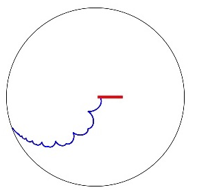
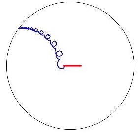
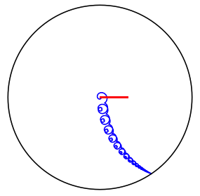
$\omega=1/2$	$\omega=1$	$\omega=3/2$
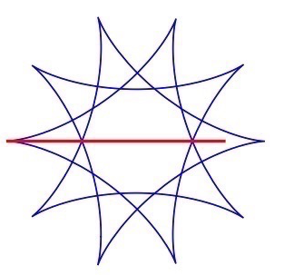
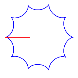
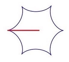
$\omega\approx 1/5$	$\omega\approx 2/5$	$\omega\approx 1/3$

Figure 6: The Mathieu equation: The space curve $\mathbf{n}$ (the horizontal segment) and the body curve $\mathbf{N}$ in the Poincaré disk model of $H^{2}$, for various choices of $\omega$ and $\epsilon$. Top row: unstable case (hyperbolic period map); bottom row: stable case (elliptic period map).

We recall briefly that the period map (the monodromy, or Floquet matrix) of equation (27) is defined by $M:=g(2\pi)\in{\mathrm{SL}_{2}(\mathbb{R})}$, where $g(t)$ is the fundamental solution of the associated linear system, and that it determines completely the stability properties of equation (27) in the sense that all solutions are bounded for all time if and only if $M$ is elliptic, or equivalently, if and only if the set of its matrix powers $\{M^{n}|n\in\mathbb{Z}\}$ is bounded. Note that for $|\epsilon|<1$, the infinitesimal generator $a(t)$ of the flow $g(t)$ of (27), for each $t$, is elliptic, and yet $M$, thought of as a composition of a non commuting family of infinitesimal elliptic rotations, may itself fail to be elliptic, leading to unbounded solutions of (27), a phenomenon known as parametric resonance [1, §25, p. 113]. Figure 8 shows the associated Arnold tongues: the shaded regions in the $(\omega,\epsilon)$–plane, corresponding to the parameter values for which the period map $M$ is hyperbolic.

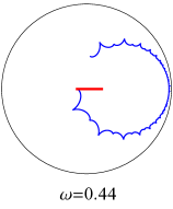
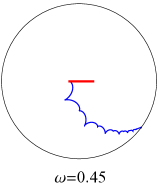
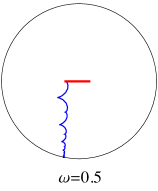
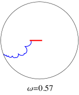
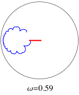
Figure 7: As $(\omega,\epsilon)$ crosses the first Arnold tongue of Figure 8 (with fixed $\epsilon=0.55)$, the curve ${\bf N}$ changes as shown, starting with the elliptic case on the left, through hyperbolic (the middle three figures) and ending an elliptic monodromy again (right) in the next stability region.

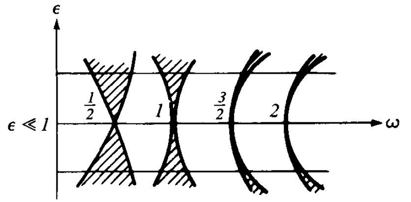
Figure 8: Arnold’s tongues for the Mathieu equation.

Returning to the hyperbolic plane $H^{2}$, Figure 7 illustrates how stability of the Mathieu equation is reflected in the body curve $\mathbf{N}(t)$: for $(\omega,\epsilon)$ in the stable (unshaded) region of Figure 8, the body curve $\mathbf{N}$ is quasi-periodic or periodic, as must be the case since the set $\{M^{n}|n\in\mathbb{Z}\}$ is bounded. On the other hand, for all resonant $(\omega,\epsilon)$ (the shaded regions of Figure 8) the body curve $\mathbf{N}$ extends to the absolute (the ‘circle at infinity’ in the Poincaré disk model of $H^{2}$ in Figure  7), reflecting the fact that the powers $M^{n}$ are unbounded as $|n|\rightarrow\infty$.

We also point out that if the period map $M$ is elliptic, conjugate to a rotation through an angle $2\pi/n$, the body curve ${\bf N}$ is closed, with $2n$ cusps, as shown in the lower row of images in Figure 6.

Figure 6 shows the ‘static’ picture, i.e., the initial position of ${\bf N}$ at $t=0$; Figures 9 and 10 illustrate the rolling of ${\bf N}$ on the space curve ${\bf n}$.

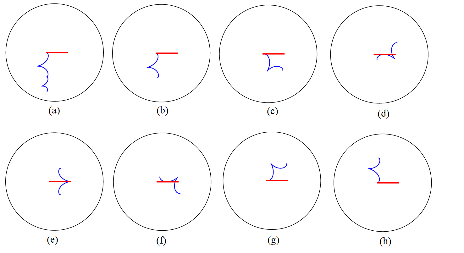
Figure 9: (a): a piece of the ‘body’ curve ${\bf N}$ and the space curve $\mathbf{n}$ (the horizontal segment) in the Poincaré disk; (b)-(h): some snapshots of a single ‘loop’ of the body curve ${\bf N}$ rolling on the space curve ${\bf n}$.

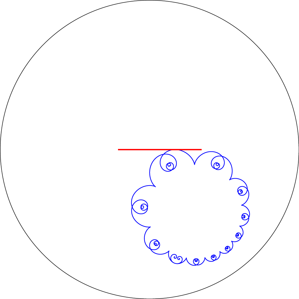
Figure 10: Another elliptic case: ${\bf N}$ rolls on ${\bf n}$.

7 Example: the bicycle equation (spacelike angular velocity)

In this section we illustrate Theorem 3 for $G={\mathrm{SL}_{2}(\mathbb{R})}$ with another example, where the motion of a ‘bicycle’ is represented by rolling of cones in Minkowski space; the bicycle is described in the caption of Figure 11.

Figure 11: The ‘bicycle’ is represented by a segment $RF$ of fixed length $\ell$ whose ‘front end’ $F$ undergoes a prescribed motion along the ‘front track’, and whose ‘rear end’ $R$ motion is constrained by the ‘no slip’ condition: its velocity is aligned with the segment $RF$ at all times.

We start by recalling the description the motion of a bicycle by a linear system of ODEs. The ‘no slip’ condition is easily seen to be equivalent to the angle $\theta$ of the bicycle satisfying

$$\ell\dot{\theta}=\dot{x}\sin\theta-\dot{y}\cos\theta,$$ (28)

where $F(t)=(x(t),y(t))$ is a parametrized ‘front track’. Equation (28) is equivalent to

$$\frac{d}{dt}\left(\begin{matrix}u\\ v\end{matrix}\right)=-{1\over 2\ell}\left(\begin{matrix}\dot{x}&\ \ \dot{y}\\ \dot{y}&-\dot{x}\end{matrix}\right)\left(\begin{matrix}u\\ v\end{matrix}\right);$$ (29)

namely, for any solution of the linear system (29), the angle

$$\theta=2\arg(u+iv)$$ (30)

evolves according to equation (28). The proof of this equivalence is a straightforward calculation (see [2, Theorem 1]).

The coefficients matrix $a(t)$ of the system (29) satisfies $\langle a,a\rangle=-4\det(a)=(\dot{x}^{2}+\dot{y}^{2})/\ell^{2}>0,$ so that $a$ is spacelike and $\mathbf{n}=a/|a|\in H^{1,1}$. From now on we assume that the front track $F(t)$ is a closed convex curve of perimeter $L$, parametrized by arc length, i.e., $|\dot{F}|^{2}=\dot{x}^{2}+\dot{y}^{2}=1$, so $\mathbf{n}=-\dot{x}\,\mathbf{i}-\dot{y}\,\mathbf{j}$ is a parametrization of the equator $x_{3}=0$ of $H^{1,1}$. In other words, the ‘space curve’ follows the equator; in particular, the geodesic curvature of $\mathbf{n}$ is $k=0$. To calculate the geodesic curvature of the body curve we use formula (26), obtaining $K=-|a|/|\dot{\mathbf{n}}|=-1/(\ell\kappa)$, where $\kappa=|\ddot{F}|=\sqrt{\ddot{x}^{2}+\ddot{y}^{2}}$ is the curvature of the front track. That is: the geodesic curvatures of the body curve $\mathbf{N}(t)\in H^{1,1}$ and the front wheel track $F(t)\in\mathbb{R}^{2}$ are reciprocal, up to a factor.

This surprising reciprocal connection between two curves living in different spaces – the bike’s front track in $\mathbb{R}^{2}$ and the body curve in $H^{1,1}$ – was proven here by computation. It turns out, however, that there is a geometrical explanation of this reciprocity; we will provide this explanation elsewhere.

We now make some observations on the body curve. Since $F(t)$ is assumed to be closed, the coefficient matrix of the bicycle system (29) is periodic; the Floquet matrix $M_{\ell}$ of this system is referred to as the $\ell$-bicycle monodromy of the front track. The monodromy $M_{\ell}$ may be elliptic, parabolic or hyperbolic; as a side remark, in the latter case $M_{\ell}$ has two real eigendirections, which correspond to two closed rear wheel tracks, as Figure 12 illustrates; one of these corresponds to the bike moving backwards.

Figure 12: Bicycle monodromy for an elliptical front track (blue): if the bicycle length $\ell$ is small enough the monodromy is hyperbolic; (a) and (b) show the two closed back tracks (red) corresponding to the two fixed point of $M_{\ell}$ in $\mathbb{R}P^{1}$. (c): for $\ell$ large enough, the monodromy is elliptic, conjugate to a rotation.

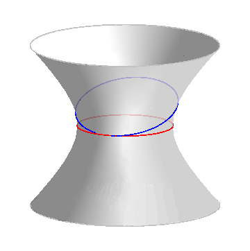
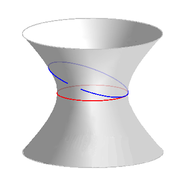
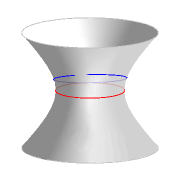
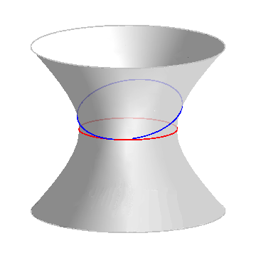
Figure 13: Some snapshots of rolling curves in $H^{1,1}$, representing bicycling along a circular front track with elliptic monodromy ($\ell>$ radius of the front track). The ‘body curve’ ${\mathbf{N}}$ (the tilted ellipse) has constant curvature $|K|>1$, and is rolling along the stationary ‘space curve’ ${\mathbf{n}}$ (the ‘equator’ of $H^{1,1}$, a geodesic).

An example. In the special case when the front track is the unit circle we have $\kappa=1$, $|K|=1/\ell$, so $\mathbf{N}$ is a spacelike constant geodesic curvature curve on $H^{1,1}$. Now all curves of constant geodesic curvature on $H^{1,1}$ are given simply by plane sections of this hyperboloid (just like in case of the ordinary sphere ${S}^{2}\subset\mathbb{R}^{3}$). In our case, the intersecting plane is tangent to the equator at $\mathbf{n}(0)$, Figure 13. For $\ell>1$ this plane section is an ellipse with geodesic curvature $|K|=1/\ell<1$, as shown in Figure 13, and the bicycle monodromy is elliptic. For $\ell=1$ the plane section is a parabola, with $|K|=1$ and $M_{\ell}$ parabolic. Similarly, for $\ell<1$ the plane section is a hyperbola, one branch of which is the body curve, with asymptotes a pair of ruling null lines of $H^{1,1}$, with $|K|=1/\ell>1$, and the bicycle monodromy is hyperbolic.

General closed front track. In the general case when $\kappa$ (the curvature of the bicycle front track $F$) is not constant and the bicycle length $\ell$ is small enough, the bicycle monodromy $M_{\ell}$ is hyperbolic and the resulting body curve $\mathbf{N}$ in $H^{1,1}$ is unbounded, asymptotic to one of the ruling null lines, as shown in Figure 14(b). For $\ell$ large enough the bicycle monodromy is elliptic and the corresponding body curve is bounded quasi-periodic, filling up a ‘ribbon’ wrapped around $H^{1,1}$, as illustrated in Figure 14(d).

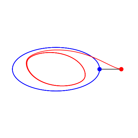
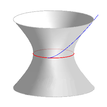
(a)		(b)
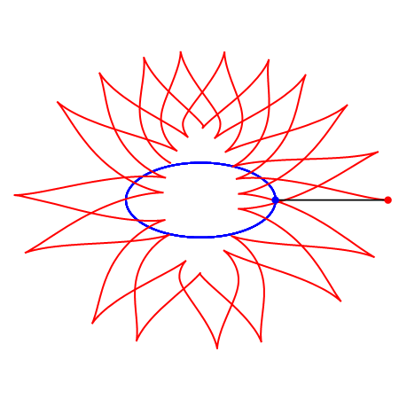
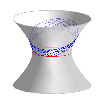
(c)		(d)

Figure 14: (a) Bicycling along an elliptical front track (blue), with hyperbolic monodromy (small $\ell$). The rear track (red) spiral towards a closed curve, corresponding to the stable fixed point of the monodromy. (b) The corresponding body curve (blue) is unbounded, asymptotic to one of the null lines on $H^{1,1}.$ (c) An elliptical front track with elliptic monodromy. The rear track is quasi-periodic. (d) The corresponding body curve is contained in a ‘ribbon’ wrapped around $H^{1,1}.$

Returning to the case of a general closed convex front track, the body curve ${\bf N}$ on $H^{1,1}$ is obtained by deforming the equator ${\bf n}$ by changing its geodesic curvature from $0$ to $1/(\ell\kappa)$; the resulting deformation “splits” what initially was the closed curve, with the endpoints and the tangents at the endpoints related by

$${\rm Ad}_{g(L)}{\bf N}(L)={\bf N}(0),\ \ {\rm Ad}_{g(L)}\dot{\bf N}(L)=\dot{\bf N}(0),$$

as Figure 13 illustrates. It turns out that the split is rather special for large $\ell$: the endpoints separate almost tangentially, as Figure 13 suggests, and the distance of separation is proportional to the area $A$ enclosed by the front track, to the leading order, as Figure 13 suggests. Indeed, this follows from the following observation.

Lemma 7.1.

Let $A$ be the area enclosed by the front track $F$. For large $\ell$, the adjoint action ${\rm Ad}_{g(L)}$ is an elliptic rotation through an angle

$$\ell^{-2}A+O(\ell^{-3}),$$ (31)

around a timelike axis which is $O(\ell^{-1})$ – close to the $a_{3}$ axis in $\mathbb{R}^{2,1}$.

In the special case when the front track is the unit circle, the picture is particularly simple, Figure 13: the body curve ${\bf N}$ is an arc of an ellipse lying in a plane tangent to the equator and of slope $\ell^{-1}$ (exactly); and the axis of the rotation ${\rm Ad}_{g(L)}$ is the line of slope $\ell$ (in the Lorenz plane the orthogonal lines have reciprocal slopes; in other words, the slope of the light line is the geometric mean of two orthogonal slopes).

Proof Lemma 7.1.

1. As stated before, we assume $F(t)$ to be a closed front track and $\ell$ to be large. According to Prytz’s formula (see [3] or [2, equation (1)]) the bicycle angle $\theta$ governed by (28) changes, after the front wheel traces out the front track, by

   $$\Delta\theta=\ell^{-2}A+O(\ell^{-3}).$$ (32)

   In particular, the rotation is near–rigid: the leading order term is independent on the initial condition $\theta(0)$.

2. According to (30), every solution $(u,v)$ of (29) rotates through half as much as $\theta$ does:

   $$\Delta\arg(u+iv)=\frac{1}{2}\Delta\theta\ \stackrel{{\scriptstyle\eqref{eq:prytz}}}{{=}}\ \frac{1}{2}\ell^{-2}A+O(\ell^{-3});$$

   and since these angles are independent of the initial condition modulo $\ell^{-3}$, we conclude that $g(L)$ is $O(\ell^{-3})$–close to the Euclidean rotation through $\frac{1}{2}\ell^{-2}A$. And this in turn implies that ${\rm Ad}_{g(L)}$ is $O(\ell^{-3})$–close to the Euclidean=Minkowski rotation $R$ around the ${\bf k}$–axis in the Minkowski space through twice the angle, namely through

   $$\ell^{-2}A+O(\ell^{-3}).$$

3. This proximity in turn implies via an implicit function argument that the the Minkowski rotation axis of ${\rm Ad}_{g(L)}$ (i.e. the eigendirection corresponding to the eigenvalue $1$) is $O(\ell^{-1})$–close to the ${\bf k}$–axis. Indeed, consider the maps induced by the linear maps ${\rm Ad}_{g(L)}$ and $R$ on the unit sphere, and examine what happens to the fixed point ${\bf k}$ of $R$ as we perturb $R$ to ${\rm Ad}_{g(L)}$. By an implicit function argument, the displacement of the fixed point is bounded by the size of the perturbation ($O(\ell^{-1})$) divided by the distance from $R$ to identity, which is at least $\frac{1}{2}\ell^{-2}A$; thus the fixed point is displaced by at most

   $$\frac{O(\ell^{-3})}{\frac{1}{2}A\ell^{-2}}=O(\ell^{-1}).$$

4. Finally, by the Minkowski orthogonality, the invariant plane of ${\rm Ad}_{g(L)}$ corresponding to the eigenvalues $\pm i\bigl{(}\ell^{-2}A+O(\ell^{-3})\bigr{)}$ has the reciprocal slope, i.e., this plane is $O(\ell^{-3})$–close to the equatorial plane. ∎

References

- [1] V.I. Arnol’d, Mathematical methods of classical mechanics. Vol. 60. Springer Science & Business Media, 2013.
- [2] G. Bor, M. Levi, R. Perline, S. Tabachnikov, Tire Tracks and Integrable Curve Evolution, Int. Math. Res. Not. IMRN (2018)
- [3] R. Foote, Geometry of the Prytz planimeter, Rep. Math. Phys. 42 (1998), 249–71.
- [4] M. Levi, Composition of rotations and parallel transport. Nonlinearity 9.2 (1996), 413.
- [5] L. Poinsot, Théorie nouvelle de la rotation des corps. Bachelier (1854).
- [6] E.T. Whittaker, A treatise on the analytical dynamics of particles and rigid bodies. Cambridge University Press, 2nd edition (1917).