Quantitative bounds for critically bounded solutions to the Navier-Stokes equations

Abstract.

We revisit the regularity theory of Escauriaza, Seregin, and Šverák for solutions to the three-dimensional Navier-Stokes equations which are uniformly bounded in the critical $L^{3}_{x}(\mathbb{R}^{3})$ norm. By replacing all invocations of compactness methods in these arguments with quantitative substitutes, and similarly replacing unique continuation and backwards uniqueness estimates by their corresponding Carleman inequalities, we obtain quantitative bounds for higher regularity norms of these solutions in terms of the critical $L^{3}_{x}$ bound (with a dependence that is triple exponential in nature). In particular, we show that as one approaches a finite blowup time $T_{*}$, the critical $L^{3}_{x}$ norm must blow up at a rate $(\log\log\log\frac{1}{T_{*}-t})^{c}$ or faster for an infinite sequence of times approaching $T_{*}$ and some absolute constant $c>0$.

1. Introduction

This paper is concerned with quantitative bounds for solutions $u:[0,T]\times\mathbb{R}^{3}\to\mathbb{R}^{3}$, $p:[0,T]\times\mathbb{R}^{3}\to\mathbb{R}$ to the Navier-Stokes equations

(1.1) $$\begin{split}\partial_{t}u+(u\cdot\nabla)u&=\Delta u-\nabla p\\ \nabla\cdot u&=0.\end{split}$$

Here we have normalised the viscosity to equal one for simplicity. To avoid technicalities, we shall restrict attention to classical solutions, by which we mean solutions that are smooth and such that all derivatives of $u,p$ lie in the space $L^{\infty}_{t}L^{2}_{x}([0,T]\times\mathbb{R}^{3})$. As our bounds are quantitative and do not depend on any smooth norms of the solution, it is possible to extend the results here to weaker notions of solution, such as mild solutions of Kato [K], the weak Leray-Hopf solutions studied in [ESS2], or the suitable weak solutions from [CKN], by using the regularity theory of such solutions; we leave the details to the interested reader. As is well known, such solutions have a maximal Cauchy development $u:[0,T_{*})\times\mathbb{R}^{3}\to\mathbb{R}^{3}$, $p:[0,T_{*})\times\mathbb{R}^{3}\to\mathbb{R}$ for some $0<T_{*}\leq\infty$, with the restriction to $[0,T]\times\mathbb{R}^{3}$ a classical solution for all $T<T_{*}$, but for which no smooth extension to time $T_{*}$ is possible if $T_{*}<\infty$. We refer to $T_{*}$ as the maximal time of existence of such a classical solution.

The Navier-Stokes system enjoys the scaling symmetry $(u,p,T)\mapsto(u^{\lambda},p^{\lambda},\lambda^{2}T)$ for any $\lambda>0$, where

$$u^{\lambda}(t,x)\coloneqq\lambda u(\lambda^{2}t,\lambda x)$$

and

$$p^{\lambda}(t,x)\coloneqq\lambda^{2}p(\lambda^{2}t,\lambda x),$$

Among other things, this means that the norm

$$\|u\|_{L^{\infty}_{t}L^{3}_{x}([0,T]\times\mathbb{R}^{3})}$$

is scale-invariant (or critical) for this equation. In [ESS2] it was shown that as long as this norm stays bounded, solutions to Navier-Stokes remain regular. In particular, they showed an endpoint of the classical Prodi-Serrin-Ladyshenskaya blowup criterion [Pr], [S2], [La] or the Leray blowup criterion [Le]:

Theorem 1.1 (Qualitative blowup criterion).

[ESS2] Suppose $(u,p)$ is a classical solution to Navier-Stokes whose maximal time of existence $T_{*}$ is finite. Then

$$\limsup_{t\to T_{*}^{+}}\|u(t)\|_{L^{3}_{x}(\mathbb{R}^{3})}=+\infty.$$

There are now many proofs, variants and generalisations [ESS2], [KK], [GKP], [GKP2], [S1], [Ph], [GIP] [DD], [A], [BS], [SS], [WZ] of this theorem, including extensions to higher dimensions or other domains than Euclidean spaces, replacing $L^{3}$ with another critical Besov or Lorenz space, or replacing the limit superior by a limit. However, in contrast to the more quantitative arguments of Leray, Prodi, Serrin and Ladyshenskaya, the proofs in the above references all rely at some point on a compactness argument to extract a limiting profile solution to which qualitative results such as unique continuation and backwards uniqueness for heat equations (as established in particular in [ESS]) can be applied. As such, the above proofs do not easily give any quantitative rate of blowup for the $L^{3}$ norm.

On the other hand, the proofs of unique continuation and backwards uniqueness rely on explicit Carleman inequalities which are fully quantitative in nature. Thus, one would expect it to be possible, at least in principle, to remove the reliance on compactness methods and obtain a quantitative version of Theorem 1.1. This is the purpose of the current paper. More precisely, in Section 6 we will establish the following two results:

Theorem 1.2 (Quantitative regularity for critically bounded solutions).

Let $u:[0,T]\times\mathbb{R}^{3}\to\mathbb{R}^{3}$, $p:[0,T]\times\mathbb{R}^{3}\to\mathbb{R}$ be a classical solution to the Navier-Stokes equations with

(1.2) $$\|u\|_{L^{\infty}_{t}L^{3}_{x}([0,T]\times\mathbb{R}^{3})}\leq A$$

for some $A\geq 2$. Then we have the derivative bounds

$$|\nabla^{j}_{x}u(t,x)|\leq\exp\exp\exp(A^{O(1)})t^{-\frac{j+1}{2}}$$

and

$$|\nabla^{j}_{x}\omega(t,x)|\leq\exp\exp\exp(A^{O(1)})t^{-\frac{j+2}{2}}$$

whenever $0<t\leq T$, $x\in\mathbb{R}^{3}$, and $j=0,1$, where $\omega\coloneqq\nabla\times u$ is the vorticity field. (See Section 2 for the asymptotic notation used in this paper.)

Remark 1.3.

It is not difficult to iterate using Schauder estimates in Hölder spaces and extend the above regularity bounds to higher values of $j$ than $j=0,1$ (allowing the implied constants in the $O()$ notation to depend on $j$), and also control time derivatives (conceding a factor of $t^{-1}$ for each time derivative); we leave this extension of Theorem 1.2 to the interested reader.

Theorem 1.4 (Quantitative blowup criterion).

Let $u:[0,T_{*})\times\mathbb{R}^{3}\to\mathbb{R}^{3}$, $p:[0,T_{*})\times\mathbb{R}^{3}\to\mathbb{R}$ be a classical solution to the Navier-Stokes equations which blows up at a finite time $0<T_{*}<\infty$. Then

$$\limsup_{t\to T_{*}^{-}}\frac{\|u(t)\|_{L^{3}_{x}(\mathbb{R}^{3})}}{(\log\log\log\frac{1}{T_{*}-t})^{c}}=+\infty$$

for an absolute constant $c>0$.

We now discuss the method of proof of these theorems, which uses many of the same key inputs as in previous arguments (most notably the Carleman estimates used to prove backwards uniqueness and unique continuation), but also introduces some other ingredients in order to avoid having to make some rather delicate results from the qualitative theory (such as profile decompositions) quantitative, as doing so would almost certainly lead to much poorer bounds than the ones given here.

The main estimate focuses on bounding the scale-invariant quantity

(1.3) $$N_{0}^{-1}|P_{N_{0}}u(t_{0},x_{0})|$$

for various points $(t_{0},x_{0})$ in spacetime, and various frequencies $N_{0}$, where $P_{N_{0}}$ is a Littlewood-Paley projection operator to frequencies $\sim N_{0}$ (see Section 2 for a precise definition). Using (1.2) and the Bernstein inequality, one can bound this quantity by $O(A)$. It is well known that if one could improve this bound somewhat for sufficiently large $N_{0}$, for instance to $O(A^{-C_{0}})$ for a large constant $C_{0}$, then (assuming $A$ is large enough) the $L^{3}$ norm becomes sufficiently “dispersed” in space and frequency that one could adapt the local well-posedness theory for the Navier-Stokes equation (or the local regularity theory from [CKN]) to obtain good bounds. Hence we will focus on establishing such a bound for (1.3) for $N_{0}$ large enough (see Theorem 5.1 for a precise statement).

The first step in doing so is to observe (basically from the Duhamel formula and some standard Littlewood-Paley theory) that if the quantity (1.3) is large for some $N_{0},t_{0},x_{0}$ with $t_{0}$ not too close to the initial time $0$, then the quantity

(1.4) $$N_{1}^{-1}|P_{N_{1}}u(t_{1},x_{1})|$$

is also large (with exactly the same lower bound) for some $(t_{1},x_{1})$ a little bit to the past of $(t_{0},x_{0})$ (but more or less within the “parabolic domain of dependence”, in the sense that $x_{1}=x_{0}+O((t_{0}-t_{1})^{1/2})$) and with $N_{1}$ comparable to $N_{0}$; see Proposition 3.1(iv) for a precise statement. If one takes care to have exactly the same lower bounds for both (1.3) and (1.4), then this claim can be iterated, creating a chain of “bubbles of concentration” at various points $(t_{n},x_{n})$ and frequencies $N_{n}$, propagating backwards in time, and for which

$$N_{n}^{-1}|P_{N_{n}}u(t_{n},x_{n})|$$

is bounded from below uniformly in $n$. Furthermore, by using a “bounded total speed” property first observed in [T], one can ensure that $(t_{n},x_{n})$ stays in the “parabolic domain of dependence” in the sense that $x_{n}=x_{0}+O((t_{0}-t_{n})^{1/2})$. Due to the well known fact (dating back to the classical work of Leray [Le]) that solutions to Navier-Stokes enjoy large “epochs of regularity” in which one has control of high regularity norms of the solution in large time intervals outside of a small dimensional singular set of times (see Proposition 3.1(iii) for a precise quantification of this statement), one can show that there are a large number of points $(t_{n},x_{n})$ for which the frequency $N_{n}$ is basically as small as possible, in the sense that

$$N_{n}\sim|t_{0}-t_{n}|^{-1/2}.$$

The (Littlewood-Paley component $P_{N_{n}}u$ of) the solution $u$ is large near $(t_{n},x_{n})$, and it is not difficult to then obtain analogous lower bounds on the vorticity

$$\omega\coloneqq\nabla\times u$$

near $(t_{n},x_{n})$. The importance of working with the vorticity comes from the fact that it obeys the vorticity equation

(1.5) $$\partial_{t}\omega=\Delta\omega-(u\cdot\nabla)\omega+(\omega\cdot\nabla)u$$

which can be viewed as a variable coefficient heat equation (in which the lower order coefficients $u,\nabla u$ depend on the velocity field) for which the non-local effects of the pressure $p$ do not explicitly appear. Using a quantitative version of unique continuation for backwards parabolic equations (see Proposition 4.3 for a precise statement) that can be established using Carleman inequalities, one can then obtain exponentially small, but still non-trivial, lower bounds for enstrophy-type quantities such as

$$\int_{I_{n}}\int_{R_{n}\leq|x-x_{n}|\leq R^{\prime}_{n}}|\omega(t,x)|^{2}\ dxdt$$

for various cylindrical annuli $I_{n}\times\{x:R_{n}\leq|x-x_{n}|\leq R^{\prime}_{n}\}$ surrounding $(t_{n},x_{n})$, with $R^{\prime}_{n}$ a large multiple of $R_{n}$. Crucially, one can set $R_{n}$ to be as large as one pleases (although the lower bound exhibits Gaussian decay in $R_{n}$). In order to apply the Carleman inequalities, it is important that the time interval $I$ lies within one of the “epochs of regularity” in which one has good $L^{\infty}$ estimates for $u,\nabla u,\omega,\nabla\omega$, but this can be accomplished without much difficulty (mainly thanks to the energy dissipation term in the energy inequality).

For many choices of scale $R_{n}$ (a bit larger than $|t_{0}-t_{n}|^{1/2}$), one can use an “energy pigeonholing argument” (as used for instance by Bourgain [B]) to make the energy (or more precisely, a certain component of the enstrophy) small in an annular region $\{x:R_{n}\leq|x-x_{n}|\leq R^{\prime}_{n}\}$ at some time $t^{\prime}_{n}$ a little bit to the past of $t_{n}$; by modifying the somewhat delicate analysis of local enstrophies from [T] that again takes advantage of the “bounded total speed” property, one can then propagate this smallness forward in time (at the cost of shrinking the annular region $\{R_{n}\leq|x-x_{n}|\leq R^{\prime}_{n}\}$ slightly), and in particular back up to time $t_{0}$, and parabolic regularity theory can then be used to obtain good $L^{\infty}$ estimates for $u,\nabla u,\omega,\nabla\omega$ in these regions. This allows us to again use Carleman inequalities. Specifically, by using the Carleman inequalities used to prove the backwards uniqueness result in [ESS2] (see Section 4 for precise statements), one can then propagate the lower bounds on $I_{n}\times\{x:R_{n}\leq|x-x_{n}|\leq R^{\prime}_{n}\}$ forward in time until one returns to the original time $t_{0}$ of interest, eventually obtaining a small but nontrivial lower bound for quantities such as

$$\int_{R_{n}\leq|x-x_{n}|\leq R^{\prime}_{n}}|\omega(t_{0},x)|^{2}\ dx$$

(ignoring for this discussion some slight adjustments to the scales $R_{n},R^{\prime}_{n}$ that occur during this argument), which after some routine manipulations (and using the fact that $(t_{n},x_{n})$ lies in the parabolic domain of dependence of $(t_{0},x_{0})$) also gives a lower bound on quantities like

$$\int_{R_{n}\leq|x-x_{0}|\leq R^{\prime}_{n}}|u(t_{0},x)|^{3}\ dx.$$

Crucially, this lower bound is uniform in $n$. If one now lets $n$ vary, the annuli $\{R_{n}\leq|x-x_{0}|\leq R^{\prime}_{n}\}$ end up becoming disjoint for widely separated $n$, and one can eventually contradict (1.2) at time $t=t_{0}$ if $N_{0}$ is large enough.

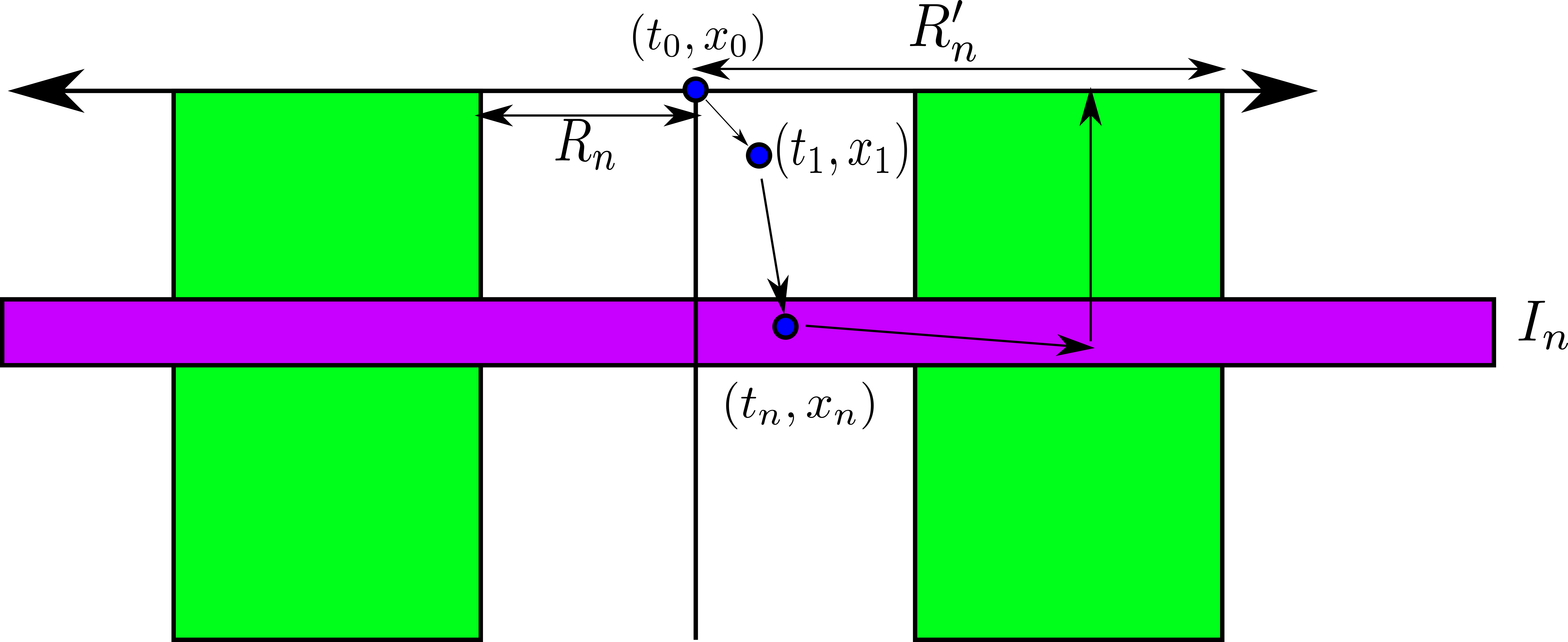
Figure 1. A schematic depiction of the main argument. Starting with a concentration of critical norm at a point $(t_{0},x_{0})$ in spacetime, one propagates this concentration backwards in time to generate concentrations at further points $(t_{n},x_{n})$ in spacetime. Restricting attention to an epoch of regularity $I_{n}\times\mathbb{R}^{3}$ (depicted here in purple), Carleman estimates are then used to establish lower bounds on the vorticity at other locations in space, and in particular where the epoch intersects an “annulus of regularity” (depicted in green) arising from an energy (or enstrophy) pigeonholing argument. A further application of Carleman estimates are then used to establish a lower bound on the vorticity (or velocity) in the annular region at time $t=t_{0}$, thus demonstrating a lack of compactness of the solution at this time which can be used to obtain a contradiction when $N_{0}$ (or more precisely the scale-invariant quantity $N_{0}^{2}T$, where $T$ is the lifespan of the solution) is large enough, by letting $n$ vary.

Remark 1.5.

The triply exponential nature of the bounds in Theorem 1.2 (which is of course closely tied to the triply logarithmic improvement to Theorem 1.1 in Theorem 1.4) can be explained as follows. One exponential factor comes from the Bourgain energy pigeonholing argument to locate a good spatial scale $R$. A second exponential factor arises from the Carleman inequalities. The third exponential arises from locating enough disjoint spatial scales $R_{n}$ to contradict (1.2). It seems that substantially new ideas would be needed in order to improve significantly upon this triple exponential bound.

Remark 1.6.

Of course, by Sobolev embedding, the $L^{3}_{x}(\mathbb{R}^{3})$ norm in the above theorems can be replaced by the critical homogeneous Sobolev norm $\dot{H}^{1/2}_{x}(\mathbb{R}^{3})$. It is likely that the arguments here can also be adapted to handle other critial Besov or Lorentz spaces (as long as the secondary exponent of such spaces is finite, so that the critical norm cannot simultaneously have a substantial presence at an unbounded number of scales), but we will not pursue this question here; based on Theorem 1.4, it is also reasonable to conjecture that the Orlicz norm $\|u(t)\|_{L^{3}(\log\log\log L)^{-c}(\mathbb{R}^{3})}$ of $u$ also must blow up as $t\to T_{*}^{-}$ for some absolute constant $c>0$. On the other hand, our argument relies heavily in many places on the fact that we are working in three dimensions. It may be possible to obtain a higher-dimensional analogue of our results by finding quantitative versions of the argument in [DD], but we do not pursue this question here. Similarly, our arguments do not directly allow us to replace the limit superior in Theorem 1.1 with a limit, as is done in [S1] (see also [A]); again, it may be possible to also find quantitative analogues of these results, but we do not pursue this matter here.

2. Notation

We use the notation $X=O(Y)$, $X\lesssim Y$, or $Y\gtrsim X$ to denote the bound $|X|\leq CY$ for some absolute constant $C>0$. If we need the implied constant $C$ to depend on parameters we shall indicate this by subscripts, for instance $X\lesssim_{j}Y$ denotes the bound $|X|\leq C_{j}Y$ where $C_{j}$ depends only on $j$.

Throughout this paper we will need a sufficiently large absolute constant $C_{0}$, which will remain fixed throughout the paper. For instance $C_{0}=10^{5}$ would suffice throughout our paper, if one worked out all the implied constants in the exponents carefully.

If $I\subset\mathbb{R}$ is a time interval, we use $|I|$ to denote its length. If $x_{0}\in\mathbb{R}^{3}$ and $R>0$, we use $B(x_{0},R)$ to denote the ball $\{x\in\mathbb{R}^{3}:|x-x_{0}|\leq R\}$, and if $B=B(x_{0},R)$ is such a ball, we use $kB=B(x_{0},kR)$ to denote its dilates for any $k>0$.

We use the mixed Lebesgue norms

$$\|u\|_{L^{q}_{t}L^{r}_{x}(I\times\mathbb{R}^{3})}\coloneqq\left(\int_{I}\|u(t)\|_{L^{r}_{x}(\mathbb{R}^{3})}^{q}\ dt\right)^{1/q}$$

where

$$\|u(t)\|_{L^{r}_{x}(\mathbb{R}^{3})}\coloneqq\left(\int_{\mathbb{R}^{3}}|u(t,x)|^{r}\ dx\right)^{1/r}$$

with the usual modifications when $q=\infty$ or $r=\infty$. For any measurable subset $\Omega\subset I\times\mathbb{R}^{3}$, we write $\|u\|_{L^{q}_{t}L^{r}_{x}(\Omega)}$ for $\|u1_{\Omega}\|_{L^{q}_{t}L^{r}_{x}(I\times\mathbb{R}^{3})}$, where $1_{\Omega}$ is the indicator function of $\Omega$.

Given a Schwartz function $f:\mathbb{R}^{3}\to\mathbb{R}$, we define the Fourier transform

$$\hat{f}(\xi)\coloneqq\int_{\mathbb{R}^{3}}f(x)e^{-2\pi i\xi\cdot x}\ dx$$

and then for any $N>0$ we define the Littlewood-Paley projection $P_{\leq N}$ by the formula

$$\widehat{P_{\leq N}f}(\xi)\coloneqq\varphi(\xi/N)\hat{f}(\xi)$$

where $\varphi:\mathbb{R}^{3}\to\mathbb{R}$ is a fixed bump function supported on $B(0,1)$ that equals $1$ on $B(0,1/2)$. We also define the companion Littlewood-Paley projections

$$P_{N} \coloneqq P_{N}-P_{N/2}$$

$$P_{>N} \coloneqq 1-P_{\leq N}$$

$$\tilde{P}_{N} \coloneqq P_{2N}-P_{N/4}$$

where $1$ denotes the identity operator; thus for instance $P_{\leq N}f=\sum_{k=0}^{\infty}P_{2^{-k}N}f$ and $P_{>N}f=\sum_{k=1}^{\infty}P_{2^{k}N}f$ for Schwartz $f$ (with the convergence in a locally uniform sense). Also we have $P_{N}=P_{N}\tilde{P}_{N}$. These operators can also be applied to vector-valued Schwartz functions by working component by component. These operators commute with other Fourier multipliers such as the Laplacian $\Delta$ and its inverse $\Delta^{-1}$, partial derivatives $\partial_{i}$, heat propagators $e^{t\Delta}$, and the Leray projection $\mathbb{P}\coloneqq-\nabla\times\Delta^{-1}\nabla\times$ to divergence-free vector fields. To estimate such multipliers, we use the following general estimate:

Lemma 2.1 (Multiplier theorem).

Let $N>0$, and let $m:\mathbb{R}^{3}\to\mathbb{C}$ be a smooth function supported on $B(0,N)$ that obeys the bounds

$$|\nabla^{j}m(\xi)|\leq MN^{-j}$$

for all $0\leq j\leq 100$ and some $M>0$. Let $T_{m}$ denote the associated Fourier multiplier, thus

$$\widehat{T_{m}f}(\xi)\coloneqq m(\xi)f(\xi).$$

Then one has

(2.1) $$\|T_{m}f\|_{L^{q}(\mathbb{R}^{3})}\lesssim MN^{\frac{3}{p}-\frac{3}{q}}\|f\|_{L^{p}(\mathbb{R}^{3})}$$

whenever $1\leq p\leq q\leq\infty$ and $f:\mathbb{R}^{3}\to\mathbb{R}$ is a Schwartz function. More generally, if $\Omega\subset\mathbb{R}^{3}$ is an open subset of $\mathbb{R}^{3}$, $A\geq 1$, and $\Omega_{A/N}\coloneqq\{x\in\mathbb{R}^{3}:\mathrm{dist}(x,\Omega)<A/N\}$ denotes the $A/N$-neighbourhood of $\Omega$, then we have a local version

(2.2) $$\|T_{m}f\|_{L^{q_{1}}(\Omega)}\lesssim MN^{\frac{3}{p_{1}}-\frac{3}{q_{1}}}\|f\|_{L^{p_{1}}(\Omega_{A/N})}+A^{-50}M|\Omega|^{\frac{1}{q_{1}}-\frac{1}{q_{2}}}N^{\frac{3}{p_{2}}-\frac{3}{q_{2}}}\|f\|_{L^{p_{2}}(\mathbb{R}^{3})}$$

of the above estimate, whenever $1\leq p_{1}\leq q_{1}\leq\infty$ and $1\leq p_{2}\leq q_{2}\leq\infty$ are such that $q_{2}\geq q_{1}$, and $|\Omega|$ denotes the volume of $\Omega$.

By the usual limiting arguments, one can replace the hypothesis that $f$ is Schwartz with the requirement that $f$ lie in $L^{p}$. Also one can extend this theorem to vector-valued $f:\mathbb{R}^{3}\to\mathbb{R}^{3}$ by working component by component. In practice, the $A^{-50}$ factor will ensure that the second term on the right-hand side of (2.2) is negligible compared to the first, and can be ignored on a first reading.

Proof.

By homogeneity we can normalise $M=1$; by scaling (or dimensional analysis) we may also normalise $N=1$. We can write $T_{m}f$ as a convolution $T_{m}f=f*K$ of $f$ with the kernel

$$K(x)\coloneqq\int_{\mathbb{R}^{3}}m(\xi)e^{2\pi i\xi\cdot x}\ d\xi.$$

By repeated integration by parts we obtain the bounds $K(x)\lesssim(1+|x|)^{-90}$ (say), so in particular $\|K\|_{L^{r}(\mathbb{R}^{3})}\lesssim 1$ for all $1\leq r\leq\infty$. From Young’s convolution inequality we then conclude that

$$\|T_{m}f\|_{L^{q}(\mathbb{R}^{3})}\lesssim\|f\|_{L^{p}(\mathbb{R}^{3})}$$

giving (2.1). To prove (2.2), we see that the claim already follows from (2.1) when $f$ is supported in $L^{p}(\Omega_{A})$, so by the triangle inequality we may assume that $f$ is supported on $\mathbb{R}^{3}\backslash\Omega_{A}$. In this case we may replace the convolution kernel $K$ by its restriction to the complement of $B(0,A)$, which allows us to improve the bound on the $L^{r}$ norm of the kernel to (say) $O(A^{-50})$. The claim follows from Young’s convolution inequality, after first using Hölder’s inequality to bound $\|T_{m}f\|_{L^{q_{1}}(\Omega)}\leq|\Omega|^{\frac{1}{q_{1}}-\frac{1}{q_{2}}}\|T_{m}f\|_{L^{q_{2}}(\Omega)}$. ∎

Thus for instance, we have the Bernstein inequalities

(2.3) $$\|\nabla^{j}f\|_{L^{q}(\mathbb{R}^{3})}\lesssim_{j}N^{j+\frac{3}{p}-\frac{3}{q}}\|f\|_{L^{p}(\mathbb{R}^{3})}$$

whenever $1\leq p\leq q\leq\infty$, $j\geq 0$, and $f$ is a Schwartz function whose Fourier transform is supported on $B(0,N)$, as can be seen by writing $f=P_{\leq 2N}f$ and applying Lemma 2.1. In a similar spirit, one has

(2.4) $$\|P_{N}e^{t\Delta}\nabla^{j}f\|_{L^{q}(\mathbb{R}^{3})}\lesssim_{j}\exp(-N^{2}t/20)N^{j+\frac{3}{p}-\frac{3}{q}}\|f\|_{L^{p}(\mathbb{R}^{3})}$$

for any $t>0$ and any Schwartz $f$. Summing this, we obtain the standard heat kernel bounds

(2.5) $$\|e^{t\Delta}\nabla^{j}f\|_{L^{q}(\mathbb{R}^{3})}\lesssim_{j}t^{-\frac{j}{2}-\frac{3}{2p}+\frac{3}{2q}}\|f\|_{L^{p}(\mathbb{R}^{3})}.$$

3. Basic estimates

The purpose of this section is to establish the following initial bounds for $L^{\infty}_{t}L^{3}_{x}$-bounded solutions to the Navier-Stokes equations.

Proposition 3.1 (Initial estimates).

Let $u:[t_{0}-T,t_{0}]\times\mathbb{R}^{3}\to\mathbb{R}^{3}$, $p:[t_{0}-T,t_{0}]\times\mathbb{R}^{3}\to\mathbb{R}$ be a classical solution to Navier-Stokes that obeys the bound

(3.1) $$\|u\|_{L^{\infty}_{t}L^{3}_{x}([t_{0}-T,t_{0}]\times\mathbb{R}^{3})}\leq A.$$

for some $A\geq C_{0}$. We adopt the notation

$$A_{j}\coloneqq A^{C_{0}^{j}}$$

for all $j$, thus $A_{0}=A$ and $A_{j+1}=A_{j}^{C_{0}}$.

• (Pointwise derivative estimates) For any $(t,x)\in[t_{0}-T/2,t_{0}]\times\mathbb{R}^{3}$ and $N>0$, we have

  (3.2) $$P_{N}u(t,x)=O(AN);\quad\nabla P_{N}u(t,x)=O(AN^{2});\quad\partial_{t}P_{N}u(t,x)=O(A^{2}N^{3});$$

  similarly, the vorticity $\omega\coloneqq\nabla\times u$ obeys the bounds

  (3.3) $$P_{N}\omega(t,x)=O(AN^{2});\quad\nabla P_{N}\omega(t,x)=O(AN^{3});\quad\partial_{t}P_{N}\omega(t,x)=O(A^{2}N^{4}).$$

• (Bounded total speed) For any interval $I$ in $[t_{0}-T/2,t_{0}]$, one has

  (3.4) $$\|u\|_{L^{1}_{t}L^{\infty}_{x}(I\times\mathbb{R}^{3})}\lesssim A^{4}|I|^{1/2}.$$

• (Epochs of regularity) For any interval $I$ in $[t_{0}-T/2,t_{0}]$, there is a subinterval $I^{\prime}\subset I$ with $|I^{\prime}|\gtrsim A^{-8}|I|$ such that

  $$\|\nabla^{j}u\|_{L^{\infty}_{t}L^{\infty}_{x}(I^{\prime}\times\mathbb{R}^{3})}\lesssim A^{O(1)}|I|^{-(j+1)/2}$$

  and

  $$\|\nabla^{j}\omega\|_{L^{\infty}_{t}L^{\infty}_{x}(I^{\prime}\times\mathbb{R}^{3})}\lesssim A^{O(1)}|I|^{-(j+2)/2}$$

  for $j=0,1$.

• (Back propagation) Let $(t_{1},x_{1})\in[t_{0}-T/2,t_{0}]\times\mathbb{R}^{3}$ and $N_{1}\geq A_{3}T^{-1/2}$ be such that

  (3.5) $$|P_{N_{1}}u(t_{1},x_{1})|\geq A_{1}^{-1}N_{1}.$$

  Then there exists $(t_{2},x_{2})\in[t_{0}-T,t_{1}]\times\mathbb{R}^{3}$ and $N_{2}\in[A_{2}^{-1}N_{1},A_{2}N_{1}]$ such that

  $$A_{3}^{-1}N_{1}^{-2}\leq t_{1}-t_{2}\leq A_{3}N_{1}^{-2}$$

  and

  $$|x_{2}-x_{1}|\leq A_{4}N_{1}^{-1}$$

  and

  (3.6) $$|P_{N_{2}}u(t_{2},x_{2})|\geq A_{1}^{-1}N_{2}.$$

• (Iterated back propagation) Let $x_{0}\in\mathbb{R}^{3}$ and $N_{0}>0$ be such that

  $$|P_{N_{0}}u(t_{0},x_{0})|\geq A_{1}^{-1}N_{0}.$$

  Then for every $A_{4}N_{0}^{-2}\leq T_{1}\leq A_{4}^{-1}T$, there exists

  $$(t_{1},x_{1})\in[t_{0}-T_{1},t_{0}-A_{3}^{-1}T_{1}]\times\mathbb{R}^{3}$$

  and

  $$N_{1}=A_{3}^{O(1)}T_{1}^{-1/2}$$

  such that

  $$x_{1}=x_{0}+O(A_{4}^{O(1)}T_{1}^{1/2})$$

  and

  $$|P_{N_{1}}u(t_{1},x_{1})|\geq A_{1}^{-1}N_{1}.$$

• (Annuli of regularity) If $0<T^{\prime}<T/2$, $x_{0}\in\mathbb{R}^{3}$, and $R_{0}\geq(T^{\prime})^{1/2}$, then there exists a scale

  $$R_{0}\leq R\leq\exp(A_{6}^{O(1)})R_{0}$$

  such that on the region

  $$\Omega:=\{(t,x)\in[t_{0}-T^{\prime},t_{0}]\times\mathbb{R}^{3}:R\leq|x-x_{0}|\leq A_{6}R\}$$

  we have

  $$\|\nabla^{j}u\|_{L^{\infty}_{t}L^{\infty}_{x}(\Omega)}\lesssim A_{6}^{-2}(T^{\prime})^{-(j+1)/2}$$

  and

  $$\|\nabla^{j}\omega\|_{L^{\infty}_{t}L^{\infty}_{x}(\Omega)}\lesssim A_{6}^{-2}(T^{\prime})^{-(j+2)/2}$$

  for $j=0,1$.

As $C_{0}$ is assumed large, any polynomial combination of $A=A_{0},A_{1},\dots,A_{j-1}$ will be dominated by $A_{j}$ for any $j\geq 1$; we take advantage of this fact without comment in the sequel to simplify the estimates. The various numerical powers of $A$ (or $A_{j}$) that appear in the above proposition are not of much significance, except that it is important for iterative purposes that the negative power $A_{1}^{-1}$ appearing in (3.5) is exactly the same as the one appearing in (3.6).

In the remainder of this section $t_{0},T,A,u,p$ are as in Proposition 3.1. Our objective is now to establish the claims (i)-(vi).

We begin with the proof of (i). It suffices to establish (3.2), as (3.3) then follows from the Bernstein inequalities (2.3). The first two claims of (3.2) are immediate from (3.1) and (2.3). For the final claim, we first apply the Leray projection $\mathbb{P}$ to (1.1) to obtain the familiar equation

(3.7) $$\partial_{t}u=\Delta u-\mathbb{P}\nabla\cdot(u\otimes u)$$

where the divergence $\nabla\cdot(u\otimes u)$ of the symmetric tensor $u\otimes u$ is expressed in coordinates as

$$(\nabla\cdot(u\otimes u))_{i}=\partial_{j}(u_{i}u_{j})$$

with the usual summation conventions. We apply $P_{N}$ to both sides of (3.7). From (3.1) and (2.3) we have

$$\|P_{N}\Delta u(t)\|_{L^{\infty}_{x}(\mathbb{R}^{3})}\lesssim N^{3}A.$$

From (3.1) and Hölder we have $\|u\otimes u(t)\|_{L^{3/2}_{x}(\mathbb{R}^{3})}\lesssim A^{2}$, hence by Lemma 2.1 we have

$$\|P_{N}\mathbb{P}\nabla\cdot(u\otimes u)(t)\|_{L^{\infty}_{x}(\mathbb{R}^{3})}\lesssim N^{3}A^{2},$$

and the final claim of (3.2) follows from the triangle inequality.

Now we prove (ii), (iii). It is not difficult to see that these estimates are invariant with respect to time translation (shifting $I,t_{0},u$ accordingly) and also rescaling (adjusting $T,t_{0},I,u$ accordingly). Hence we may assume without loss of generality that $I=[0,1]\subset[t_{0}-T/2,t_{0}]$, which implies that $[-1,1]\subset[t_{0}-T,t_{0}]$.

It will be convenient to remove a linear component from $u$, as it is not well controlled in $L^{2}_{x}$ type spaces. Namely, on $[-1,1]\times\mathbb{R}^{3}$ we split $u=u^{\operatorname{lin}}+u^{\operatorname{nlin}}$, where $u^{\operatorname{lin}}$ is the linear solution

(3.8) $$u^{\operatorname{lin}}(t)\coloneqq e^{(t+1)\Delta}u(-1)$$

and $u^{\operatorname{nlin}}\coloneqq u-u^{\operatorname{lin}}$ is the nonlinear component. From (3.1) we have

(3.9) $$\|u^{\operatorname{lin}}\|_{L^{\infty}_{t}L^{3}_{x}([-1,1]\times\mathbb{R}^{3})},\|u^{\operatorname{nlin}}\|_{L^{\infty}_{t}L^{3}_{x}([-1,1]\times\mathbb{R}^{3})}\lesssim A.$$

From (3.7) and Duhamel’s formula one has

$$u^{\operatorname{nlin}}(t)=-\int_{-1}^{t}e^{(t-t^{\prime})\Delta}\mathbb{P}\nabla\cdot(u\otimes u)(t^{\prime})\ dt^{\prime}.$$

From (3.1), $u\otimes u$ has an $L^{3/2}_{x}(\mathbb{R}^{3})$ norm of $O(A^{2})$. From (2.5), the operator $e^{(t-t^{\prime})\Delta}\mathbb{P}\nabla\cdot$ maps $L^{3/2}_{x}$ to $L^{2}_{x}$ with an operator norm of $(t-t^{\prime})^{-3/4}$. From Minkowski’s inequality we conclude an energy bound for the nonlinear component:

(3.10) $$\|u^{\operatorname{nlin}}\|_{L^{\infty}_{t}L^{2}_{x}([-1,1]\times\mathbb{R}^{3})}\lesssim A^{2}.$$

We now restrict attention to the slab $[-1/2,1]\times\mathbb{R}^{3}$. Here $t+1$ lies between $1/2$ and $2$, and we can use (3.1), (3.8), and (2.5) to obtain very good bounds on $u^{\operatorname{lin}}$ (but only in spaces with an integrability exponent greater than or equal to $3$). More precisely, we have

(3.11) $$\|\nabla^{j}u^{\operatorname{lin}}\|_{L^{\infty}_{t}L^{p}_{x}([-1/2,1]\times\mathbb{R}^{3})}\lesssim_{j}A$$

for any $3\leq p\leq\infty$ and $j\geq 0$.

To exploit the bound (3.10), we use the energy method. Since $u^{\operatorname{lin}}$ solves the heat equation $\partial_{t}u^{\operatorname{lin}}=\Delta u^{\operatorname{lin}}$, we can subtract this from (1.1) to conclude that

(3.12) $$\partial_{t}u^{\operatorname{nlin}}=\Delta u^{\operatorname{nlin}}-\nabla\cdot(u\otimes u)-\nabla p.$$

Taking inner products with $u^{\operatorname{nlin}}$, which is divergence-free, and integrating by parts, we conclude that

$$\frac{1}{2}\partial_{t}\int_{\mathbb{R}^{3}}|u^{\operatorname{nlin}}|^{2}\ dx=-\int_{\mathbb{R}^{3}}|\nabla u^{\operatorname{nlin}}|^{2}\ dx+\int_{\mathbb{R}^{3}}(\nabla u^{\operatorname{nlin}})\cdot(u\otimes u)\ dx$$

where the quantity $(\nabla u^{\operatorname{nlin}})\cdot(u\otimes u)$ is defined in coordinates as

$$(\nabla u^{\operatorname{nlin}})\cdot(u\otimes u)\coloneqq(\partial_{i}u^{\operatorname{nlin}}_{j})u_{i}u_{j}.$$

From the divergence-free nature of $u^{\operatorname{nlin}}$ and integration by parts we have

$$\int_{\mathbb{R}^{3}}(\nabla u^{\operatorname{nlin}})\cdot(u^{\operatorname{nlin}}\otimes u^{\operatorname{nlin}})\ dx=0$$

and hence

$$\frac{1}{2}\partial_{t}\int_{\mathbb{R}^{3}}|u^{\operatorname{nlin}}|^{2}\ dx=-\int_{\mathbb{R}^{3}}|\nabla u^{\operatorname{nlin}}|^{2}\ dx+\int_{\mathbb{R}^{3}}(\nabla u^{\operatorname{nlin}})\cdot(u\otimes u-u^{\operatorname{nlin}}\otimes u^{\operatorname{nlin}})\ dx.$$

Integrating this on $[-1/2,1]$ using (3.10) we conclude that

$$\int_{-1/2}^{1}\int_{\mathbb{R}^{3}}|\nabla u^{\operatorname{nlin}}|^{2}\ dxdt\lesssim A^{2}+\int_{-1/2}^{1}\int_{\mathbb{R}^{3}}|\nabla u^{\operatorname{nlin}}||u\otimes u-u^{\operatorname{nlin}}\otimes u^{\operatorname{nlin}}|\ dxdt,$$

and hence by Young’s inequality

$$\int_{-1/2}^{1}\int_{\mathbb{R}^{3}}|\nabla u^{\operatorname{nlin}}|^{2}\ dxdt\lesssim A^{2}+\int_{-1/2}^{1}\int_{\mathbb{R}^{3}}|u\otimes u-u^{\operatorname{nlin}}\otimes u^{\operatorname{nlin}}|^{2}\ dxdt.$$

Splitting $u\otimes u-u^{\operatorname{nlin}}\otimes u^{\operatorname{nlin}}=u_{l}\otimes u+u^{\operatorname{nlin}}\otimes u_{l}$ and using (3.1), (3.9), (3.11) (with $p=6$, $j=0$) and Hölder’s inequality, one has

$$\int_{-1/2}^{1}\int_{\mathbb{R}^{3}}|u\otimes u-u^{\operatorname{nlin}}\otimes u^{\operatorname{nlin}}|^{2}\ dxdt\lesssim A^{4}$$

and thus

(3.13) $$\int_{-1/2}^{1}\int_{\mathbb{R}^{3}}|\nabla u^{\operatorname{nlin}}|^{2}\ dxdt\lesssim A^{4}.$$

By Plancherel’s theorem this implies in particular that

(3.14) $$\sum_{N}N^{2}\|P_{N}u^{\operatorname{nlin}}\|_{L^{2}_{t}L^{2}_{x}([-1/2,1]\times\mathbb{R}^{3})}^{2}\lesssim A^{4}$$

where $N$ ranges over powers of two. Also, from Sobolev embedding one has

(3.15) $$\|u^{\operatorname{nlin}}\|_{L^{2}_{t}L^{6}_{x}([-1/2,1]\times\mathbb{R}^{3})}\lesssim A^{2}.$$

We are now ready to establish the bounded total speed property (ii), which is a variant of [T, Proposition 9.1]. If $t\in[0,1]$ and $N\geq 1$ is a power of two, we see from (3.7) and Duhamel’s formula that

$$P_{N}u^{\operatorname{nlin}}(t)=e^{(t+\frac{1}{2})\Delta}P_{N}u^{\operatorname{nlin}}\left(-\frac{1}{2}\right)-\int_{-1/2}^{t}P_{N}e^{(t-t^{\prime})\Delta}\mathbb{P}\nabla\cdot\tilde{P}_{N}(u\otimes u)(t^{\prime})\ dt^{\prime}.$$

From (2.4) the operator $P_{N}e^{(t-t^{\prime})\Delta}\mathbb{P}\nabla\cdot$ has an operator norm of $O(N\exp(-N^{2}(t-t^{\prime})/20))$ on $L^{\infty}_{x}$, while from (3.9), (2.4) we see that $e^{(t+\frac{1}{2})\Delta}P_{N}v(-\frac{1}{2})$ has an $L^{\infty}_{x}$ norm of $O(AN\exp(-N^{2}/20))$. Thus by Young’s inequality

$$\|P_{N}u^{\operatorname{nlin}}\|_{L^{1}_{t}L^{\infty}_{x}([0,1]\times\mathbb{R}^{3})}\lesssim AN\exp(-N^{2}/20)+N^{-1}\|\tilde{P}_{N}(u\otimes u)\|_{L^{1}_{t}L^{\infty}_{x}([-1/2,1]\times\mathbb{R}^{3})}.$$

We split $u\otimes u=u^{\operatorname{lin}}\otimes u^{\operatorname{lin}}+u^{\operatorname{lin}}\otimes u^{\operatorname{nlin}}+u^{\operatorname{nlin}}\otimes u^{\operatorname{lin}}+u^{\operatorname{nlin}}\otimes u^{\operatorname{nlin}}$. From (3.11) one has

$$\|\tilde{P}_{N}(u^{\operatorname{lin}}\otimes u^{\operatorname{lin}})\|_{L^{1}_{t}L^{\infty}_{x}([-1/2,1]\times\mathbb{R}^{3})}\lesssim A^{2}.$$

From (2.3), Hölder’s inequality, and (3.11), (3.15) one has

$$\|\tilde{P}_{N}(u^{\operatorname{lin}}\otimes u^{\operatorname{nlin}})\|_{L^{1}_{t}L^{\infty}_{x}([-1/2,1]\times\mathbb{R}^{3})} \lesssim N^{1/2}\|u^{\operatorname{lin}}\otimes u^{\operatorname{nlin}}\|_{L^{1}_{t}L^{6}_{x}([-1/2,1]\times\mathbb{R}^{3})}$$

$$\lesssim A^{3}N^{1/2}.$$

Similarly with $u^{\operatorname{lin}}\otimes u^{\operatorname{nlin}}$ replaced by $u^{\operatorname{nlin}}\otimes u^{\operatorname{lin}}$. We then split $u^{\operatorname{nlin}}\otimes u^{\operatorname{nlin}}=P_{\leq N}u^{\operatorname{nlin}}\otimes P_{\leq N}u^{\operatorname{nlin}}+P_{\leq N}u^{\operatorname{nlin}}\otimes P_{>N}u^{\operatorname{nlin}}+P_{>N}u^{\operatorname{nlin}}\otimes P_{\leq N}u^{\operatorname{nlin}}+P_{>N}u^{\operatorname{nlin}}\otimes P_{>N}u^{\operatorname{nlin}}$. We have from Hölder that

$$\|P_{\leq N}u^{\operatorname{nlin}}\otimes P_{\leq N}u^{\operatorname{nlin}}\|_{L^{1}_{t}L^{\infty}_{x}([-1/2,1]\times\mathbb{R}^{3})} \lesssim\|P_{\leq N}u^{\operatorname{nlin}}\|_{L^{2}_{t}L^{\infty}_{x}([-1/2,1]\times\mathbb{R}^{3})}^{2}$$

$$\|P_{\leq N}u^{\operatorname{nlin}}\otimes P_{>N}u^{\operatorname{nlin}}\|_{L^{1}_{t}L^{2}_{x}([-1/2,1]\times\mathbb{R}^{3})},\quad$$

$$\|P_{>N}u^{\operatorname{nlin}}\otimes P_{\leq N}u^{\operatorname{nlin}}\|_{L^{1}_{t}L^{2}_{x}([-1/2,1]\times\mathbb{R}^{3})} \lesssim\|P_{\leq N}u^{\operatorname{nlin}}\|_{L^{2}_{t}L^{\infty}_{x}([-1/2,1]\times\mathbb{R}^{3})}$$

$$\quad\times\|P_{>N}u^{\operatorname{nlin}}\|_{L^{2}_{t}L^{2}_{x}([-1/2,1]\times\mathbb{R}^{3})}$$

$$\|P_{>N}u^{\operatorname{nlin}}\otimes P_{>N}u^{\operatorname{nlin}}\|_{L^{1}_{t}L^{1}_{x}([-1/2,1]\times\mathbb{R}^{3})} \lesssim\|P_{>N}u^{\operatorname{nlin}}\|_{L^{2}_{t}L^{2}_{x}([-1/2,1]\times\mathbb{R}^{3})}^{2}$$

and hence by (2.3), the triangle inequality, and Young’s inequality

$$\|\tilde{P}_{N}(u\otimes u)\|_{L^{1}_{t}L^{\infty}_{x}([-1/2,1]\times\mathbb{R}^{3})}\lesssim\|P_{\leq N}u^{\operatorname{nlin}}\|_{L^{2}_{t}L^{\infty}_{x}([-1/2,1]\times\mathbb{R}^{3})}^{2}+N^{3}\|P_{>N}u^{\operatorname{nlin}}\|_{L^{2}_{t}L^{2}_{x}([-1/2,1]\times\mathbb{R}^{3})}^{2}.$$

Putting all this together, we conclude that

$$\|P_{N}u^{\operatorname{nlin}}\|_{L^{1}_{t}L^{\infty}_{x}([0,1]\times\mathbb{R}^{3})} \lesssim A^{3}N^{-1/2}$$

$$\quad+N^{-1}\|P_{\leq N}u^{\operatorname{nlin}}\|_{L^{2}_{t}L^{\infty}_{x}([-1/2,1]\times\mathbb{R}^{3})}^{2}$$

$$\quad+N^{2}\|P_{>N}u^{\operatorname{nlin}}\|_{L^{2}_{t}L^{2}_{x}([-1/2,1]\times\mathbb{R}^{3})}^{2}.$$

By (2.3) and Cauchy-Schwarz we have

$$\|P_{\leq N}u^{\operatorname{nlin}}\|_{L^{2}_{t}L^{\infty}_{x}([-1/2,1]\times\mathbb{R}^{3})}^{2} \lesssim\left(\sum_{N^{\prime}\leq N}(N^{\prime})^{3/2}\|P_{N^{\prime}}u^{\operatorname{nlin}}\|_{L^{2}_{t}L^{2}_{x}([-1/2,1]\times\mathbb{R}^{3})}\right)^{2}$$

$$\lesssim N^{1/2}\sum_{N^{\prime}\leq N}(N^{\prime})^{2}\|P_{N^{\prime}}u^{\operatorname{nlin}}\|_{L^{2}_{t}L^{2}_{x}([-1/2,1]\times\mathbb{R}^{3})}^{2}$$

where $N^{\prime}$ ranges over powers of two, while from Plancherel’s theorem one has

$$\|P_{>N}u^{\operatorname{nlin}}\|_{L^{2}_{t}L^{2}_{x}([-1/2,1]\times\mathbb{R}^{3})}^{2}\lesssim\sum_{N^{\prime}>N}\|P_{N^{\prime}}u^{\operatorname{nlin}}\|_{L^{2}_{t}L^{2}_{x}([-1/2,1]\times\mathbb{R}^{3})}^{2}.$$

Summing in $N$, and using the triangle inequality followed by (3.14), we conclude that

$$\|P_{\geq 1}u^{\operatorname{nlin}}\|_{L^{1}_{t}L^{\infty}_{x}([0,1]\times\mathbb{R}^{3})}\lesssim A^{3}+\sum_{N^{\prime}}(N^{\prime})^{2}\|P_{N^{\prime}}u^{\operatorname{nlin}}\|_{L^{2}_{t}L^{2}_{x}([-1/2,1]\times\mathbb{R}^{3})}^{2}\lesssim A^{4}.$$

From (3.9) and (2.3) we also have

$$\|u^{\operatorname{lin}}\|_{L^{1}_{t}L^{\infty}_{x}([0,1]\times\mathbb{R}^{3})},\|P_{<1}u^{\operatorname{nlin}}\|_{L^{1}_{t}L^{\infty}_{x}([0,1]\times\mathbb{R}^{3})}\lesssim A$$

and we conclude

$$\|u\|_{L^{1}_{t}L^{\infty}_{x}([0,1]\times\mathbb{R}^{3})}\lesssim A^{4}$$

which gives (ii).

Now we establish (iii). For $t\in[0,1]$ we define the enstrophy-type quantity

$$E(t)\coloneqq\frac{1}{2}\int_{\mathbb{R}^{3}}|\nabla u^{\operatorname{nlin}}(t,x)|^{2}\ dx,$$

Taking the gradient of (3.12) and then taking the inner product with $\nabla u^{\operatorname{nlin}}$, we see upon integration by parts that

$$\partial_{t}E(t)=-\int_{\mathbb{R}^{3}}|\nabla^{2}u^{\operatorname{nlin}}|^{2}\ dx+\int_{\mathbb{R}^{3}}\Delta u^{\operatorname{nlin}}\cdot(\nabla\cdot(u\otimes u))\ dx$$

and hence by Young’s inequality

$$\partial_{t}E(t)\leq-\frac{1}{2}\|\nabla^{2}u^{\operatorname{nlin}}\|_{L^{2}_{x}(\mathbb{R}^{3})}^{2}+O\left(\|\nabla\cdot(u\otimes u)\|_{L^{2}_{x}(\mathbb{R}^{3})}^{2}\right).$$

By the Leibniz rule and Hölder’s inequality, one has

$$\|\nabla\cdot(u\otimes u)\|_{L^{2}_{x}(\mathbb{R}^{3})}\lesssim\|u\|_{L^{6}_{x}(\mathbb{R}^{3})}\|\nabla u\|_{L^{3}_{x}(\mathbb{R}^{3})}.$$

From (3.11) and the triangle inequality one has

$$\|u\|_{L^{6}_{x}(\mathbb{R}^{3})}\lesssim A+\|u^{\operatorname{nlin}}\|_{L^{6}_{x}(\mathbb{R}^{3})}$$

and

$$\|\nabla u\|_{L^{3}_{x}(\mathbb{R}^{3})}\lesssim A+\|\nabla u^{\operatorname{nlin}}\|_{L^{3}_{x}(\mathbb{R}^{3})}$$

while from Sobolev embedding and Hölder one has

$$\|u^{\operatorname{nlin}}\|_{L^{6}_{x}(\mathbb{R}^{3})}\lesssim\|\nabla u^{\operatorname{nlin}}\|_{L^{2}_{x}(\mathbb{R}^{3})}\lesssim E(t)^{1/2}$$

and

$$\|\nabla u^{\operatorname{nlin}}\|_{L^{3}_{x}(\mathbb{R}^{3})}\lesssim\|\nabla u^{\operatorname{nlin}}\|_{L^{2}_{x}(\mathbb{R}^{3})}^{1/2}\|\nabla^{2}u^{\operatorname{nlin}}\|_{L^{2}_{x}(\mathbb{R}^{3})}^{1/2}\lesssim E(t)^{1/4}\|\nabla^{2}u^{\operatorname{nlin}}\|_{L^{2}_{x}(\mathbb{R}^{3})}^{1/2}.$$

We conclude that

$$\partial_{t}E(t)\leq-\frac{1}{2}\|\nabla^{2}u^{\operatorname{nlin}}\|_{L^{2}_{x}(\mathbb{R}^{3})}^{2}+O\left((A^{2}+E(t))(A^{2}+E(t)^{1/2}\|\nabla^{2}u^{\operatorname{nlin}}\|_{L^{2}_{x}(\mathbb{R}^{3})})\right)$$

and hence by Young’s inequality

(3.16) $$\partial_{t}E(t)\leq-\frac{1}{4}\|\nabla^{2}u^{\operatorname{nlin}}\|_{L^{2}_{x}(\mathbb{R}^{3})}^{2}+O((A^{2}+E(t))A^{2}+(A^{2}+E(t))^{2}E(t)).$$

In particular we have

(3.17) $$\partial_{t}E(t)\leq O(A^{4}+A^{4}E(t)+E(t)^{3}).$$

From (3.13) we have

$$\int_{0}^{1}E(t)\ dt\lesssim A^{4},$$

and hence by the pigeonhole principle, we can find a time $t_{1}\in[0,1/2]$ such that

$$E(t_{1})\lesssim A^{4}.$$

A standard continuity argument using (3.17) then gives $E(t)\lesssim A^{4}$ for $t\in[t_{1},t_{1}+cA^{-8}]=[\tau(0),\tau(1)]$, where $\tau(s)\coloneqq t_{1}+scA^{-8}$ and $c>0$ is a small absolute constant. Inserting this back into (3.16) one has

$$\partial_{t}E(t)\leq-\frac{1}{4}\|\nabla^{2}u^{\operatorname{nlin}}\|_{L^{2}_{x}(\mathbb{R}^{3})}^{2}+O(A^{12})$$

and hence by the fundamental theorem of calculus

(3.18) $$\int_{\tau(0)}^{\tau(1)}\int_{\mathbb{R}^{3}}|\nabla^{2}u^{\operatorname{nlin}}|^{2}\ dxdt\lesssim A^{4}.$$

Thus we have

(3.19) $$\|\nabla u^{\operatorname{nlin}}\|_{L^{\infty}_{t}L^{2}_{x}([\tau(0),\tau(1)]\times\mathbb{R}^{3})}+\|\nabla^{2}u^{\operatorname{nlin}}\|_{L^{2}_{t}L^{2}_{x}([\tau(0),\tau(1)]\times\mathbb{R}^{3})}\lesssim A^{2}.$$

From the Gagliardo-Nirenberg inequality

(3.20) $$\|u^{\operatorname{nlin}}\|_{L^{\infty}_{x}}\lesssim\|\nabla u^{\operatorname{nlin}}\|_{L^{2}_{x}}^{1/2}\|\nabla^{2}u^{\operatorname{nlin}}\|_{L^{2}_{x}}^{1/2}$$

and Hölder’s inequality, one concludes in particular that

$$\|u^{\operatorname{nlin}}\|_{L^{4}_{t}L^{\infty}_{x}([\tau(0),\tau(1)]\times\mathbb{R}^{3})}\lesssim A^{2}$$

and hence by (3.11)

(3.21) $$\|u\|_{L^{4}_{t}L^{\infty}_{x}([\tau(0),\tau(1)]\times\mathbb{R}^{3})}\lesssim A^{2};$$

also from Sobolev embedding and (3.19) one has

$$\|\nabla u^{\operatorname{nlin}}\|_{L^{2}_{t}L^{6}_{x}([\tau(0),\tau(1)]\times\mathbb{R}^{3})}\lesssim A^{2}$$

and hence by (3.11)

(3.22) $$\|\nabla u\|_{L^{2}_{t}L^{6}_{x}([\tau(0),\tau(1)]\times\mathbb{R}^{3})}\lesssim A^{2}.$$

These are subcritical regularity estimates and can now be iterated to obtain even higher regularity. For $t\in[\tau(0.1),\tau(1)]$, we see from (3.7) that

(3.23) $$u(t)=e^{(t-\tau(0))\Delta}u(\tau(0))-\int_{\tau(0)}^{t}e^{(t-t^{\prime})\Delta}\mathbb{P}\nabla\cdot(u\otimes u)(t^{\prime})\ dt^{\prime}.$$

From (2.5) the operator $e^{(t-t^{\prime})\Delta}\mathbb{P}\nabla\cdot$ has norm $O((t-t^{\prime})^{-1/2})$ on $L^{\infty}_{x}$, while $e^{(t-\tau(0))\Delta}$ maps $L^{3}_{x}$ to $L^{\infty}_{x}$ with norm $O((t-\tau(0))^{-1/2})=O(A^{O(1)})$. We conclude from (3.1) that

$$\|u(t)\|_{L^{\infty}_{x}(\mathbb{R}^{3})}\lesssim A^{O(1)}+\int_{\tau(0)}^{t}(t-t^{\prime})^{-1/2}\|u(t)\|_{L^{\infty}_{x}(\mathbb{R}^{3})}^{2}\ dt^{\prime}.$$

From (3.21) and Young’s convolution inequality, we conclude that

$$\|u\|_{L^{8}_{t}L^{\infty}_{x}([\tau(0.1),\tau(1)]\times\mathbb{R}^{3})}\lesssim A^{O(1)}$$

Repeating the above argument, we now also see for $t\in[\tau(0.2),\tau(1)]$ that

$$\|u(t)\|_{L^{\infty}_{x}(\mathbb{R}^{3})}\lesssim A^{O(1)}+\int_{\tau(0.1)}^{t}(t-t^{\prime})^{-1/2}\|u(t)\|_{L^{\infty}_{x}(\mathbb{R}^{3})}^{2}\ dt^{\prime}$$

so from Hölder’s inequality we conclude that

(3.24) $$\|u\|_{L^{\infty}_{t}L^{\infty}_{x}([\tau(0.2),\tau(1)]\times\mathbb{R}^{3})}\lesssim A^{O(1)}.$$

Now we differentiate (3.7) to conclude that

$$\nabla u(t)=\nabla e^{(t-\tau(0.2))\Delta}u(\tau(0.2))-\int_{\tau(0.2)}^{t}\nabla e^{(t-t^{\prime})\Delta}\mathbb{P}\nabla\cdot(u\otimes u)(t^{\prime})\ dt^{\prime}$$

for $t\in[\tau(0.3),\tau(1)]$. From (3.1), the first term $\nabla e^{(t-\tau(0.2))\Delta}u(\tau(0.2))$ has an $L^{\infty}_{x}$ norm of $O(A^{O(1)})$. From (2.5), the operator $\nabla e^{(t-t^{\prime})\Delta}\mathbb{P}$ maps $L^{6}_{x}$ to $L^{\infty}_{x}$ with norm $O((t-t^{\prime})^{-3/4})$, thus

$$\|\nabla u(t)\|_{L^{\infty}_{x}(\mathbb{R}^{3})}\lesssim A^{O(1)}+\int_{\tau(0.2)}^{t}(t-t^{\prime})^{-3/4}\|\nabla\cdot(u\otimes u)(t^{\prime})\|_{L^{6}_{x}(\mathbb{R}^{3})}\ dt^{\prime}.$$

From (3.22), (3.24), Leibniz and Hölder one has

$$\|\nabla\cdot(u\otimes u)\|_{L^{2}_{t}L^{6}_{x}([\tau(0.2),\tau(1)]\times\mathbb{R}^{3})}\lesssim A^{O(1)}$$

and hence by fractional integration

$$\|\nabla u\|_{L^{4}_{t}L^{\infty}_{x}([\tau(0.3),\tau(1)]\times\mathbb{R}^{3})}\lesssim A^{O(1)}.$$

From this, (3.24), Leibniz, and Hölder one has

$$\|\nabla\cdot(u\otimes u)\|_{L^{4}_{t}L^{\infty}_{x}([\tau(0.3),\tau(1)]\times\mathbb{R}^{3})}\lesssim A^{O(1)}.$$

By (2.5), $\nabla e^{(t-t^{\prime})\Delta}\mathbb{P}$ has an operator norm of $O((t-t^{\prime})^{-1/2})$ on $L^{\infty}_{x}$, thus

$$\|\nabla u(t)\|_{L^{\infty}_{x}(\mathbb{R}^{3})}\lesssim A^{O(1)}+\int_{\tau(0.3)}^{t}(t-t^{\prime})^{-1/2}\|\nabla\cdot(u\otimes u)(t^{\prime})\|_{L^{\infty}_{x}(\mathbb{R}^{3})}\ dt^{\prime}$$

for $t\in[\tau(0.4),\tau(1)]$, and hence by Hölder’s inequality

$$\|\nabla u\|_{L^{\infty}_{t}L^{\infty}_{x}([\tau(0.4),\tau(1)]\times\mathbb{R}^{3})}\lesssim A^{O(1)}.$$

From the vorticity equation (1.5), we now have

$$\partial_{t}\omega=\Delta\omega+O(A^{O(1)}(|\omega|+|\nabla\omega|))$$

on $[\tau(0.4),\tau(1)]\times\mathbb{R}^{3}$, and also $\omega=O(A^{O(1)})$ on this slab. Standard parabolic regularity estimates (see e.g., [LSU]) then give

$$\|\nabla\omega\|_{L^{\infty}_{t}L^{\infty}_{x}([\tau(0.5),\tau(1)]\times\mathbb{R}^{3})}\lesssim A^{O(1)}.$$

Setting $I^{\prime}\coloneqq[\tau(0.5),\tau(1)]$, we obtain the claim (iii). We remark that it is also possible to control higher derivatives $\nabla^{j}u,\nabla^{j}\omega$ with $j>1$, for instance by using parabolic Schauder estimates in Hölder spaces, but we will not need to do so here.

Now we establish (iv). Let $t_{1},x_{1},N_{1}$ be as in that part of the proposition. By rescaling we may normalise $N_{1}=1$, and by translation invariance we may normalise $(t_{1},x_{1})=(0,0)$, so that $t_{0}-T\leq-\frac{T}{2}\leq-\frac{A_{3}^{2}}{2}$, so in particular $[-2A_{3},0]\subset[t_{0}-T,t_{0}]$. From (3.5) we have

(3.25) $$|P_{1}u(0,0)|\geq A_{1}^{-1}.$$

Assume for contradiction that the claim fails, then we have

$$\|P_{N}u\|_{L^{\infty}_{t}L^{\infty}_{x}([-A_{3},-A_{3}^{-1}]\times B(0,A_{4}))}\leq A_{1}^{-1}N$$

for all $A_{2}^{-1}\leq N\leq A_{2}$. From (3.2) and the fundamental theorem of calculus in time, we can enlarge the time interval to reach $t=0$, so that

$$\|P_{N}u\|_{L^{\infty}_{t}L^{\infty}_{x}([-A_{3},0]\times B(0,A_{4}))}\lesssim A_{1}^{-1}N.$$

Suppose now that $N\geq A_{2}^{-1}$. For $t\in[-A_{3},0]$, we can use Duhamel’s formula, (3.7), and the triangle inequality to write

$$\|P_{N}u(t)\|_{L^{3/2}_{x}(B(0,A_{4}))} \leq\|e^{(t+2A_{3})\Delta}P_{N}u(-2A_{3})\|_{L^{3/2}_{x}(B(0,A_{4}))}$$

$$\quad+\int_{-2A_{3}}^{t}\|e^{(t-t^{\prime})\Delta}P_{N}\nabla\cdot(u(t^{\prime})\otimes u(t^{\prime}))\|_{L^{3/2}_{x}(\mathbb{R}^{3})}\ dt^{\prime}.$$

From (2.4), $e^{(t+2A_{3})\Delta}P_{N}$ has an operator norm of $O(\exp(-N^{2}A_{3}/20))$ on $L^{3}_{x}$, and $e^{(t-t^{\prime})\Delta}P_{N}\nabla\cdot$ similarly has an operator norm of $O(N\exp(-N^{2}(t-t^{\prime})/20))$ on $L^{3/2}_{x}$. Applying (3.1) and Hölder’s inequality, we conclude that

$$\|P_{N}u(t)\|_{L^{3/2}_{x}(B(0,A_{4}))}\lesssim AA_{4}\exp(-N^{2}A_{3}/20)+A^{2}N^{-1}$$

and hence in the range $N\geq A_{2}^{-1}$ we have

(3.26) $$\|P_{N}u\|_{L^{\infty}_{t}L^{3/2}_{x}([-A_{3},0]\times B(0,A_{4}))}\lesssim A^{2}N^{-1}.$$

Now suppose that $N\geq A_{2}^{-1/2}$. For $t\in[-A_{3}/2,0]$, we again use Duhamel’s formula, (3.7) and the triangle inequality to write

$$\|P_{N}u(t)\|_{L^{1}_{x}(B(0,A_{4}/2))} \leq\|e^{(t+A_{3})\Delta}P_{N}u(-A_{3})\|_{L^{1}_{x}(B(0,A_{4}/2))}$$

$$\quad+\int_{-A_{3}}^{t}\|e^{(t-t^{\prime})\Delta}P_{N}\nabla\cdot\tilde{P}_{N}(u(t^{\prime})\otimes u(t^{\prime}))\|_{L^{1}_{x}(B(0,A_{4}/2))}\ dt^{\prime}.$$

From (2.4), (3.1), and Hölder as before we have

$$\|e^{(t+A_{3})\Delta}P_{N}u(-A_{3})\|_{L^{1}_{x}(B(0,A_{4}/2))}\lesssim AA_{4}^{2}\exp(-N^{2}A_{3}/40).$$

From (2.2) one has

$$\|e^{(t-t^{\prime})\Delta}P_{N}\nabla\cdot\tilde{P}_{N}(u(t^{\prime})\otimes u(t^{\prime}))\|_{L^{1}_{x}(B(0,A_{4}/2))}\lesssim N\exp(-N^{2}(t-t^{\prime})/20)$$

$$\quad\times\left(\|\tilde{P}_{N}(u(t^{\prime})\otimes u(t^{\prime}))\|_{L^{1}_{x}(B(0,3A_{4}/4)}+A_{4}^{-50}A_{4}^{1/2}\|\tilde{P}_{N}(u(t^{\prime})\otimes u(t^{\prime}))\|_{L^{3/2}_{x}(\mathbb{R}^{3})}\right)$$

and hence by (3.1)

$$\|P_{N}u\|_{L^{\infty}_{t}L^{1}_{x}([-A_{3}/2,0]\times B(0,A_{4}/2))}\lesssim A_{4}^{-40}+N^{-1}\|\tilde{P}_{N}(u(t^{\prime})\otimes u(t^{\prime}))\|_{L^{\infty}_{t}L^{1}_{x}([-A_{3},0]\times B(0,3A_{4}/4))}.$$

Since $\tilde{P}_{N}(P_{\leq N/100}u(t^{\prime})\otimes P_{\leq N/100}u(t^{\prime}))$ vanishes, we can write

(3.27) $$\tilde{P}_{N}(u(t^{\prime})\otimes u(t^{\prime}))=\tilde{P}_{N}(P_{>N/100}u(t^{\prime})\otimes u(t^{\prime}))+\tilde{P}_{N}(P_{\leq N/100}u(t^{\prime})\otimes P_{>N/100}u(t^{\prime})).$$

From (2.2), (3.1) we have

$$\|\tilde{P}_{N}(P_{>N/100}u(t^{\prime})\otimes u(t^{\prime}))\|_{L^{\infty}_{t}L^{1}_{x}([-A_{3},0]\times B(0,3A_{4}/4))}\lesssim\|P_{>N/100}u(t^{\prime})\otimes u(t^{\prime})\|_{L^{\infty}_{t}L^{1}_{x}([-A_{3},0]\times B(0,A_{4}))}+A_{4}^{-40}.$$

From (3.26) (and the triangle inequality) as well as (3.1) and Hölder’s inequality, we thus have

$$\|\tilde{P}_{N}(P_{>N/100}u(t^{\prime})\otimes u(t^{\prime}))\|_{L^{\infty}_{t}L^{1}_{x}([-A_{3},0]\times B(0,3A_{4}/4))}\lesssim A^{3}N^{-1}.$$

Similarly for the other component of (3.27). We conclude that

(3.28) $$\|P_{N}u\|_{L^{\infty}_{t}L^{1}_{x}([-A_{3}/2,0]\times B(0,A_{4}/2))}\lesssim A^{3}N^{-2}$$

for all $N\geq A_{2}^{-1/2}$.

Now suppose that $A_{2}^{-1/3}\leq N\leq A_{2}^{1/3}$. For $t\in[-A_{3}/3,0]$, we again use Duhamel’s formula, (3.7), and the triangle inequality as before to write

$$\|P_{N}u(t)\|_{L^{2}_{x}(B(0,A_{4}/4))}\leq\|e^{(t+A_{3}/2)\Delta}P_{N}u(-A_{3}/2)\|_{L^{2}_{x}(B(0,A_{4}/4))}$$

$$\quad+\int_{-A_{3}/2}^{t}\|e^{(t-t^{\prime})\Delta}P_{N}\nabla\cdot\tilde{P}_{N}(u(t^{\prime})\otimes u(t^{\prime}))\|_{L^{2}_{x}(B(0,A_{4}/4))}\ dt^{\prime}.$$

Arguing as before we have

$$\|e^{(t+A_{3}/2)\Delta}P_{N}u(-A_{3}/2)\|_{L^{2}_{x}(B(0,A_{4}/4))}\lesssim AA_{4}^{1/2}\exp(-N^{2}A_{3}/120)$$

and

$$\|e^{(t-t^{\prime})\Delta}P_{N}\nabla\cdot\tilde{P}_{N}(u(t^{\prime})\otimes u(t^{\prime}))\|_{L^{2}_{x}(B(0,A_{4}/4))}\lesssim N^{5/2}\exp(-N^{2}(t-t^{\prime})/20)$$

$$\quad\left(\|\tilde{P}_{N}(u(t^{\prime})\otimes u(t^{\prime}))\|_{L^{1}_{x}(B(0,A_{4}/3))}+A_{4}^{-50}N^{-1}\|\tilde{P}_{N}(u(t^{\prime})\otimes u(t^{\prime}))\|_{L^{3/2}_{x}(\mathbb{R}^{3})}\right)$$

and thus

(3.29) $$\|P_{N}u\|_{L^{\infty}_{t}L^{2}_{x}([-A_{3}/4,0]\times B(0,A_{4}/4))}\lesssim A_{4}^{-40}+N^{1/2}\|\tilde{P}_{N}(u(t^{\prime})\otimes u(t^{\prime}))\|_{L^{\infty}_{t}L^{1}_{x}([-A_{3}/2,0]\times B(0,A_{4}/3))}.$$

We can split $\tilde{P}_{N}(u(t^{\prime})\otimes u(t^{\prime}))$ into $O(1)$ paraproduct terms of the form $\tilde{P}_{N}(P_{N^{\prime}}u(t^{\prime})\otimes P_{\leq N/100}u(t^{\prime}))$ where $N^{\prime}\sim N$, $O(1)$ terms of the form $\tilde{P}_{N}(P_{\leq N/100}u(t^{\prime})\otimes P_{N^{\prime}}u(t^{\prime}))$, and a sum of the form $\sum_{N_{1}\sim N_{2}\gtrsim N}\tilde{P}_{N}(P_{N_{1}}u(t^{\prime})\otimes P_{N_{2}}u(t^{\prime}))$. For the “high-low” term $\tilde{P}_{N}(P_{N^{\prime}}u(t^{\prime})\otimes P_{\leq N/100}u(t^{\prime}))$, we observe from (3.26), (3.2) and the triangle inequality that

$$\|P_{\leq N/100}u\|_{L^{\infty}_{t}L^{3/2}_{x}([-A_{3},0]\times B(0,A_{4}))}\lesssim A^{2}N^{-1}.$$

Using this, (2.2), (3.28) (for the high frequency factor $P_{N^{\prime}}u(t^{\prime})$), and Hölder’s inequality, we conclude that the contribution of this term to (3.29) is $O(A^{3}A_{1}^{-1}N^{-1/2})$. Similarly for the “low-high” term $\tilde{P}_{N}(P_{\leq N/100}u(t^{\prime})\otimes P_{N^{\prime}}u(t^{\prime}))$. Finally, to control the “high-high” term $\sum_{N_{1}\sim N_{2}\gtrsim N}\tilde{P}_{N}(P_{N_{1}}u(t^{\prime})\otimes P_{N_{2}}u(t^{\prime}))$, we use (2.2), the triangle inequality, Hölder, and (3.28) to control this contribution by

$$\lesssim A_{4}^{-40}+N^{1/2}\sum_{N_{1}\sim N_{2}\gtrsim N}A^{3}N_{1}^{-2}\|P_{N_{2}}u\|_{L^{\infty}_{t}L^{3/2}_{x}([-A_{3},0]\times B(0,A_{4}))}.$$

Using (3.26) when $N_{2}\leq A_{2}$ and (3.2) otherwise, we see that this term also contributes $O(A^{3}A_{1}^{-1}N^{-1/2})$. We have thus shown that

(3.30) $$\|P_{N}u\|_{L^{\infty}_{t}L^{2}_{x}([-A_{3}/4,0]\times B(0,A_{4}/4))}\lesssim A^{3}A_{1}^{-1}N^{-1/2}$$

for $A_{2}^{-1/3}\leq N\leq A_{2}^{1/3}$.

We now return once again to Duhamel’s formula to estimate

$$|P_{1}u(0,0)|\leq|e^{A_{3}\Delta/4}P_{1}u(-A_{3}/4)|(0)+\int_{-A_{3}/4}^{0}|e^{(t-t^{\prime})\Delta}P_{1}\nabla\cdot\tilde{P}_{1}(u(t^{\prime})\otimes u(t^{\prime}))|(0)\ dt^{\prime}.$$

From (2.4), (3.1), the first term is $O(A_{3}\exp(-A_{3}^{2}/320))$, thus from (3.25) we have

$$\int_{-A_{3}/4}^{0}|e^{(t-t^{\prime})\Delta}P_{1}\nabla\cdot\tilde{P}_{1}(u(t^{\prime})\otimes u(t^{\prime}))|(0)\ dt^{\prime}\gtrsim A_{1}^{-1}.$$

From (2.2), (3.1) one has

$$|e^{(t-t^{\prime})\Delta}P_{1}\nabla\cdot\tilde{P}_{1}(u(t^{\prime})\otimes u(t^{\prime}))|(0)\lesssim\exp(-(t-t^{\prime})/20)(\|\|\tilde{P}_{1}(u(t^{\prime})\otimes u(t^{\prime}))\|_{L^{1}_{x}(B(0,A_{1}))}+A_{1}^{-50})$$

and hence by the pigeonhole principle we have

$$\|\tilde{P}_{1}(u(t^{\prime})\otimes u(t^{\prime}))\|_{L^{1}_{x}(B(0,A_{1}))}\gtrsim A_{1}^{-1}.$$

for some $-A_{3}/4\leq t^{\prime}\leq 0$.

Fix this $t^{\prime}$. As before, we can split $\tilde{P}_{1}(u(t^{\prime})\otimes u(t^{\prime}))$ into the sum of $O(1)$ “low-high” terms $\tilde{P}_{1}(P_{N^{\prime}}u(t^{\prime})\otimes P_{\leq 1/100}u(t^{\prime}))$ and “high-low” terms $\tilde{P}_{1}(P_{\leq 1/100}u(t^{\prime})\otimes P_{N^{\prime}}u(t^{\prime}))$ with $N^{\prime}\sim 1$, plus a “high-high” term $\sum_{N_{1}\sim N_{2}\gtrsim 1}\tilde{P}_{1}(P_{N_{1}}u(t^{\prime})\otimes P_{N_{2}}u(t^{\prime}))$. For the first two types of terms, we use (2.2) (for frequencies larger than $A_{2}^{-1/3}$), (3.1), and Hölder to conclude that

$$\|P_{\leq 100}u(t^{\prime})\|_{L^{2}_{x}(B(0,2A_{1}))}\lesssim A^{3}A_{1}^{-1}$$

and then from (3.30), (2.2) (and (3.1) to control the global contribution of (2.2)) we see that the contribution of those two types of terms is $O(A^{6}A_{1}^{-2})$. For the high-high terms with $N_{1},N_{2}\leq A_{2}^{1/3}$, we again use (3.30), (2.2), (3.1) to again obtain a bound of $O(A^{6}A_{1}^{-2})$. For the cases when $N_{1},N_{2}\gtrsim A_{2}^{1/3}$, we use (3.26), (3.1) to obtain a much better bound $O(A^{3}A_{2}^{-1/3})$. Putting all this together we obtain

$$A_{1}^{-1}\lesssim A^{6}A_{1}^{-2}$$

giving the required contradiction. This establishes (iv).

Now we prove (v). We may assume that $A_{4}N_{0}^{-2}\leq A_{4}^{-1}T$, since the claim is trivial otherwise. Thus we have $N_{0}\geq A_{4}T^{-1/2}$.

By iteratively applying (iv), we may find a sequence $(t_{0},x_{0}),(t_{1},x_{1}),\dots,(t_{n},x_{n})\in[t_{0}-T,t_{0}]$ and $N_{0},N_{1},\dots,N_{n}>0$ for some $n\geq 1$, with the properties

(3.31) $$|P_{N_{i}}u(t_{i},x_{i})| \geq A_{1}^{-1}N_{i}$$

(3.32) $$A_{2}^{-1}N_{i-1} \leq N_{i}\leq A_{2}N_{i-1}$$

(3.33) $$A_{3}^{-1}N_{i-1}^{-2} \leq t_{i-1}-t_{i}\leq A_{3}N_{i-1}^{-2}$$

(3.34) $$|x_{i}-x_{i-1}| \leq A_{4}N_{i-1}^{-1}$$

for all $i=1,\dots,n$, with $t_{i}\in[t_{0}-T/2,t_{0}]$ and $N_{i}\geq A_{3}T^{-1/2}$ for $i=0,\dots,n-1$ and either $t_{n}\in[t_{0}-T,t_{0}-T/2]$ or $N_{n}<A_{3}T^{-1/2}$. To see that this process terminates at a finite $n$, observe from the classical nature of $u$ that the $P_{N_{i}}u(t_{i},x_{i})$ are uniformly bounded in $i$, which by (3.31) implies that the $N_{i}$ are uniformly bounded above, and hence by (3.33) $t_{i-1}-t_{i}$ are uniformly bounded below; since $t_{i}$ must stay above $t_{0}-T$, we obtain the required finite time termination. By (3.33), the first time $t_{1}$ after $t_{0}$ lies in the interval

$$t_{1}\in[t_{0}-A_{2}N_{0}^{-2},t_{0}-A_{2}^{-1}N_{0}^{-2}].$$

If $N_{n}<A_{3}T^{-1/2}$, then by (3.33), (3.32)

$$t_{n-1}-t_{n}\geq A_{3}^{-1}N_{n-1}^{-2}\geq A_{3}^{-2}N_{n}^{-2}\geq A_{3}^{-4}(t_{n-1}-t_{n})\leq A_{3}^{-4}T$$

so in particular $t_{n}\leq t_{0}-A_{3}^{-4}T$. Of course this inequality also holds if $t_{n}\in[t_{0}-T,t_{0}-T/2]$. In either case, we see from the hypothesis $A_{4}N_{0}^{-2}\leq T_{1}\leq A_{4}^{-1}T$ that

$$t_{n}<t-T_{1}\leq t_{1}.$$

Let $m$ be the largest index for which $t_{m}\geq t-T_{1}$, thus $1\leq m\leq n-1$ and $t_{m+1}>t-T_{1}$. By telescoping (3.33), we conclude that

(3.35) $$\sum_{i=0}^{m}A_{3}N_{i}^{-2}=\sum_{i=1}^{m+1}A_{3}N_{i-1}^{-2}\geq t-t_{m+1}\geq T_{1}.$$

On the other hand, from (3.31) and (3.2) we have

$$|P_{N_{i}}u(t,x_{i})|\gtrsim A_{1}^{-1}N_{i}$$

for $t\in[t_{i}-A_{1}^{-2}N_{i}^{-2},t_{i}]$; as $P_{N_{i}}$ is bounded on $L^{\infty}$ by (2.3), this implies that

$$\|P_{N_{i}}u(t)\|_{L^{\infty}_{x}(\mathbb{R}^{3})}\gtrsim A_{1}^{-1}N_{i}$$

for such $t$. From (3.33) we see that the time intervals $[t_{i}-A_{1}^{-2}N_{i}^{-2},t_{i}]$ are disjoint and lie in $[t-T_{1},t]$ for $i=0,\dots,m-1$. Applying (3.4), we conclude that

$$\sum_{i=0}^{m-1}A_{1}^{-1}N_{i}\times A_{1}^{-2}N_{i}^{-2}\lesssim A^{4}T_{1}^{1/2}$$

and thus

$$\sum_{i=0}^{m-1}N_{i}^{-1}\lesssim A_{1}^{4}T_{1}^{1/2}.$$

Using (3.32) to extend this sum to the final index $m$, we conclude that

(3.36) $$\sum_{i=0}^{m}N_{i}^{-1}\lesssim A_{2}^{2}T_{1}^{1/2}.$$

Comparing this with (3.35), we conclude that there exists $i=0,\dots,m$ such that

$$N_{i}^{-1}\gtrsim A_{3}^{-2}T_{1}^{1/2}.$$

Since $A_{4}N_{0}^{-2}\leq A_{4}^{-1}T$, $i$ cannot be zero, thus $1\leq i\leq m$. From (3.33), (3.32) we have

$$t_{0}-t_{i} \geq t_{i-1}-t_{i}$$

$$\geq A_{3}^{-1}N_{i-1}^{-2}$$

$$\geq A_{3}^{-2}N_{i}^{-2}$$

$$\gtrsim A_{3}^{-6}T_{1}.$$

Since $t_{0}-t_{i}$ is also bounded by $T_{1}$, we also have from (3.33) that $A_{3}^{-1}N_{i}^{-2}\leq T_{1}$, thus $N_{i}\geq A_{3}^{-1/2}T_{1}^{-1/2}$. Finally, from telescoping (3.34) and using (3.36), we conclude that

$$|x_{i}-x_{0}|\lesssim A_{4}^{2}T_{1}^{1/2},$$

and the claim follows.

Finally, we prove (vi), which is the most difficult estimate. The claim is invariant with respect to time translation and rescaling, so we may assume that $[t_{0}-T^{\prime},t_{0}]=[0,1]$. In particular $[-1,1]\subset[t_{0}-T,t_{0}]$, so we may decompose $u=u^{\operatorname{lin}}+u^{\operatorname{nlin}}$ as before with the estimates (3.10), (3.11), (3.13).

From (3.13) we can find a time $t_{1}\in[-1/2,0]$ such that

$$\int_{\mathbb{R}^{3}}|\nabla u^{\operatorname{nlin}}(t_{1},x)|^{2}\ dx\lesssim A^{4}.$$

Fix this time $t_{1}$. From (3.11) we thus have

$$\int_{\mathbb{R}^{3}}|\nabla u^{\operatorname{nlin}}(t_{1},x)|^{2}+\sum_{j=0}^{4}|\nabla^{j}u^{\operatorname{lin}}(t_{1},x)|^{3}\ dx\lesssim A^{4}.$$

By the pigeonhole principle, we can thus find a scale

(3.37) $$A_{6}^{100}R_{0}\leq R\leq\exp(A_{6}^{O(1)})R_{0}$$

such that

(3.38) $$\int_{A_{6}^{-10}R\leq|x|\leq A_{6}^{10}R}|\nabla u^{\operatorname{nlin}}(t_{1},x)|^{2}+\sum_{j=0}^{4}|\nabla^{j}u^{\operatorname{lin}}(t_{1},x)|^{3}\ dx\lesssim A_{6}^{-10}.$$

Fix this $R$. We now propagate this estimate forward in time to $[t_{1},1]$. We first achieve this for the linear component $u^{\operatorname{lin}}$, which is straightforward. From Sobolev embedding we have

$$\sup_{A_{6}^{-9}R\leq|x|\leq A_{6}^{9}R}|\nabla^{j}u^{\operatorname{lin}}(t_{1},x)|\lesssim A_{6}^{-3}$$

for $j=0,1,2$. Since $\nabla^{j}u^{\operatorname{lin}}$ solves the linear heat equation, we conclude from this, (2.2), and (3.11) that

(3.39) $$\sup_{t_{1}\leq t\leq 1}\sup_{A_{6}^{-8}R\leq|x|\leq A_{6}^{8}R}|\nabla^{j}u^{\operatorname{lin}}(t,x)|\lesssim A_{6}^{-3}$$

for $j=0,1,2$. This estimate (when combined with (3.11)) will suffice to control all the terms involving the linear component $u^{\operatorname{lin}}$ of the velocity (or the analogous component $\omega^{\operatorname{lin}}\coloneqq\nabla\times u^{\operatorname{lin}}$ of the vorticity).

The vorticity $\omega\coloneqq\nabla\times u$ obeys the vorticity equation (1.5). On $[t_{1},1]\times\mathbb{R}^{3}$, we decompose $\omega=\omega^{\operatorname{lin}}+\omega^{\operatorname{nlin}}$, where $\omega^{\operatorname{lin}}\coloneqq\nabla\times u^{\operatorname{lin}}$ is the linear component of the vorticity and $\omega^{\operatorname{nlin}}\coloneqq\nabla\times u^{\operatorname{nlin}}$ is the nonlinear component. As $\omega^{\operatorname{lin}}$ solves the heat equation, we have

(3.40) $$\partial_{t}\omega^{\operatorname{nlin}}=\Delta\omega^{\operatorname{nlin}}-(u\cdot\nabla)\omega+(\omega\cdot\nabla)u.$$

As in [T, §10], we apply the energy method to this equation with a carefully chosen time-dependent cutoff function. Namely, let

(3.41) $$R_{-}\in[A_{6}^{-8}R,2A_{6}^{-8}R];\quad R_{+}\in[A_{6}^{8}R/2,A_{6}^{8}R]$$

be scales to be chosen later, and define the time-dependent radii

$$R_{-}(t) \coloneqq R_{-}+C_{0}\int_{t_{1}}^{t}(A_{6}+\|u(t)\|_{L^{\infty}_{x}(\mathbb{R}^{3})})\ dt$$

$$R_{+}(t) \coloneqq R_{+}-C_{0}\int_{t_{1}}^{t}(A_{6}+\|u(t)\|_{L^{\infty}_{x}(\mathbb{R}^{3})})\ dt$$

that start at $R_{-},R_{+}$ respectively, and contract inwards at a rate faster than the velocity field $u$. From the bounded total speed property (3.4), (3.37), and the hypothesis $R_{0}\geq 1$, we conclude that

$$R_{-}(t)\in[A_{6}^{-8}R,3A_{6}^{-8}R];\quad R_{+}(t)\in[A_{6}^{8}R/3,A_{6}^{8}R]$$

for all $t\in[t_{1},1]$.

For $t\in[t_{1},1]$, we define the local enstrophy

$$E(t)\coloneqq\frac{1}{2}\int_{\mathbb{R}^{3}}|\omega^{\operatorname{nlin}}(t,x)|^{2}\eta(t,x)\ dx$$

where $\eta$ is the time-varying cutoff

$$\eta(t,x)\coloneqq\max(\min(A_{6},|x|-R_{-}(t),R_{+}(t)-|x|),0),$$

thus $\eta$ is supported in the annulus $\{R_{-}(t)\leq|x|\leq R_{+}(t)\}$, is Lipschitz with norm $1$, and equals $A_{6}$ in the smaller annulus $\{R_{-}(t)+A_{6}\leq|x|\leq R_{+}(t)-A_{6}\}$. From (3.38) we have the initial bound

(3.42) $$E(t_{1})\lesssim A_{6}^{-9}.$$

Now we control the time derivative $\partial_{t}E(t)$ for $t\in[t_{1},1]$. From (3.40) and integration by parts we have

$$\partial_{t}E(t)=-Y_{1}(t)-Y_{2}(t)+Y_{3}(t)+Y_{4}(t)+Y_{5}(t)+Y_{6}(t)+Y_{7}(t)+Y_{8}(t)+Y_{9}(t)$$

where $Y_{1}$ is the dissipation term

$$Y_{1}(t)\coloneqq\int_{\mathbb{R}^{3}}|\nabla\omega^{\operatorname{nlin}}(t,x)|^{2}\ dx,$$

$Y_{2}(t)$ is the recession term

$$Y_{2}(t)\coloneqq-\frac{1}{2}\int_{\mathbb{R}^{3}}|\omega^{\operatorname{nlin}}(t,x)|^{2}\partial_{t}\eta(t,x)\ dx,$$

$Y_{3}(t)$ is the heat flux term

$$Y_{3}(t)\coloneqq\frac{1}{2}\int_{\mathbb{R}^{3}}|\omega^{\operatorname{nlin}}(t,x)|^{2}\Delta\eta(t,x)\ dx,$$

$Y_{4}(t)$ is the transport term

$$Y_{4}(t)\coloneqq\frac{1}{2}\int_{\mathbb{R}^{3}}|\omega^{\operatorname{nlin}}(t,x)|^{2}u(t,x)\cdot\nabla\eta(t,x)\ dx,$$

$Y_{5}(t)$ is a correction to the transport term arising from $\omega^{\operatorname{lin}}$,

$$Y_{5}(t)\coloneqq-\int_{\mathbb{R}^{3}}\omega^{\operatorname{nlin}}(t,x)\cdot(u(t,x)\cdot\nabla)\omega^{\operatorname{lin}}(t,x)\ \eta(t,x)\ dx,$$

$Y_{6}(t)$ is the main nonlinear term

$$Y_{6}(t)\coloneqq\int_{\mathbb{R}^{3}}\omega^{\operatorname{nlin}}(t,x)\cdot(\omega^{\operatorname{nlin}}(t,x)\cdot\nabla)u^{\operatorname{nlin}}(t,x)\ \eta(t,x)\ dx$$

and $Y_{7}(t),Y_{8}(t),Y_{9}(t)$ are corrections to the transport term arising from the $u^{\operatorname{lin}}$ and $\omega^{\operatorname{lin}}$,

$$Y_{7}(t) \coloneqq\int_{\mathbb{R}^{3}}\omega^{\operatorname{nlin}}(t,x)\cdot(\omega^{\operatorname{nlin}}(t,x)\cdot\nabla)u^{\operatorname{lin}}(t,x)\ \eta(t,x)\ dx$$

$$Y_{8}(t) \coloneqq\int_{\mathbb{R}^{3}}\omega^{\operatorname{nlin}}(t,x)\cdot(\omega^{\operatorname{lin}}(t,x)\cdot\nabla)u^{\operatorname{nlin}}(t,x)\ \eta(t,x)\ dx$$

$$Y_{9}(t) \coloneqq\int_{\mathbb{R}^{3}}\omega^{\operatorname{nlin}}(t,x)\cdot(\omega^{\operatorname{lin}}(t,x)\cdot\nabla)u^{\operatorname{lin}}(t,x)\ \eta(t,x)\ dx.$$

Here all derivatives of the Lipschitz function $\eta$ are interpreted in a distributional sense. We now aim to control $Y_{3}(t),\dots,Y_{9}(t)$ in terms of $Y_{1}(t),Y_{2}(t),E(t)$, and some other quantities that are well controlled. From definition of $\eta$ we see that

$$-\partial_{t}\eta(t,x)=C_{0}(A_{6}+\|u(t)\|_{L^{\infty}_{x}(\mathbb{R}^{3})})|\nabla\eta(t,x)|$$

so in particular we have that $Y_{2}(t)$ is non-negative and

$$Y_{4}(t)\leq C_{0}^{-1}Y_{2}(t).$$

A direct computation of $\Delta\eta$ in polar coordinates yields the bound

$$Y_{3}(t) \lesssim\int_{|x|\in[R_{-}(t),R_{-}(t)+A_{6}]\cup[R_{+}(t)-A_{6},R_{+}(t)]}\frac{|\omega^{\operatorname{nlin}}(t,x)|^{2}}{|x|}\ dx$$

$$\quad+\sum_{r=R_{-}(t),R_{-}(t)+A_{6},R_{+}(t)-A_{6},R_{+}(t)}r^{2}\int_{S^{2}}|\omega^{\operatorname{nlin}}(t,r\theta)|\ d\theta$$

where $d\theta$ is surface measure on the sphere (in fact the $r=R_{-}(t)+A_{6},R_{+}(t)-A_{6}$ terms are non-positive and could be discarded if desired). This expression is difficult to estimate for fixed choices of $R_{-},R_{+}$. However, if selects $R_{-},R_{+}$ uniformly at random from the range (3.41), we see from Fubini’s theorem that the expected value $\mathbb{E}|Y_{3}|$ of $|Y_{3}|$ can be estimated by

$$\mathbb{E}|Y_{3}(t)|\lesssim A_{6}\int_{|x|\in[A_{6}^{-8}R,3A_{6}^{-8}R]\cup[A_{6}^{8}R/3,A_{6}^{8}R]}\frac{|\omega^{\operatorname{nlin}}(t,x)|^{2}}{|x|^{2}}\ dx$$

and hence by (3.13), (3.37)

$$\mathbb{E}\int_{t_{1}}^{1}|Y_{3}(t)|\ dt\lesssim A_{6}^{-10}$$

(say). Thus we can select $R_{-},R_{+}$ so that

(3.43) $$\int_{t_{1}}^{1}|Y_{3}(t)|\ dt\lesssim A_{6}^{-10}$$

and we shall now do so.

To treat $Y_{5}(t)$, we use Young’s inequality to bound

$$Y_{5}(t)\lesssim E(t)+\int_{\mathbb{R}^{3}}|(u\cdot\nabla)\omega^{\operatorname{lin}}|^{2}\ \eta\ dx.$$

Using (3.1), (3.11), (3.39), Hölder’s inequality, we then have

$$Y_{5}(t)\lesssim E(t)+A_{6}^{-2}$$

(say).

In a similar vein, from (3.39) and Hölder’s inequality one has

$$Y_{7}(t)\lesssim E(t)$$

(with plenty of room to spare) and from Young’s inequality one has

$$Y_{9}(t)\lesssim E(t)+\int_{\mathbb{R}^{3}}|(\omega^{\operatorname{lin}}\cdot\nabla)u^{\operatorname{lin}}|^{2}\ \eta(t,x)\ dx$$

and hence by (3.1), (3.11), (3.39), and Hölder

$$Y_{9}(t)\lesssim E(t)+A_{6}^{-2}.$$

For $Y_{8}$, we again use Young’s inequality to bound

$$Y_{8}(t)\lesssim E(t)+\int_{\mathbb{R}^{3}}|(\omega^{\operatorname{lin}}\cdot\nabla)u^{\operatorname{nlin}}|^{2}\ \eta(t,x)\ dx$$

and hence by (3.39)

$$Y_{8}(t)\lesssim E(t)+Y_{10}(t)$$

where

$$Y_{10}(t)\coloneqq A_{6}^{-3}\int_{\mathbb{R}^{3}}|\nabla u^{\operatorname{nlin}}(t,x)|^{2}\ dx.$$

Observe from (3.13) that

(3.44) $$\int_{t_{1}}^{1}|Y_{10}(t)|\ dt\lesssim A_{6}^{-2}.$$

We are left with estimation of the most difficult term $Y_{6}(t)$. Following [T], we cover the annulus $\{R_{-}(t)\leq|x|\leq R_{+}(t)\}$ by a boundedly overlapping Whitney decomposition of balls $B=B(x_{B},r_{B})$, where the radius $r_{B}$ of the ball is given as $r_{B}\coloneqq\frac{1}{100}\eta(t,r_{B})$. In particular, we have $\eta(t,x)\sim r_{B}$ on the dilate $10B=B(x_{B},r_{B})$ of the ball. We can then write

$$Y_{6}(t)\sim\sum_{B}r_{B}\int_{B}|\omega^{\operatorname{nlin}}|^{2}|\nabla u^{\operatorname{nlin}}|\ dx$$

where we suppress the explicit dependence on $t,x$ for brevity. Similarly one has

(3.45) $$E(t)\sim\sum_{B}r_{B}\int_{10B}|\omega^{\operatorname{nlin}}|^{2}\ dx$$

and

(3.46) $$Y_{1}(t)\sim\sum_{B}r_{B}\int_{10B}|\nabla\omega^{\operatorname{nlin}}|^{2}\ dx$$

To control $Y_{6}(t)$, we need to control $\nabla u^{\operatorname{nlin}}$. The Biot-Savart law suggests that this function has comparable size to $\omega^{\operatorname{nlin}}$, but we need to localise this intuition to the ball $B$ and thus must address the slightly non-local nature of the Biot-Savart law. Fortunately this can be handled using standard cutoff functions. Namely, we have $\Delta u^{\operatorname{nlin}}=-\nabla\times\omega^{\operatorname{nlin}}$, hence if we let $\psi_{B}$ be a smooth cutoff adapted to $3B$ that equals $1$ on $2B$, then

$$u^{\operatorname{nlin}}=-\Delta^{-1}(\nabla\times(\omega^{\operatorname{nlin}}\psi_{B}))+v$$

where $v$ is harmonic on $2B$. From Sobolev embedding and Hölder one has

$$\|v\|_{L^{2}_{x}(2B)}\lesssim\|\omega^{\operatorname{nlin}}\psi_{B}\|_{L^{6/5}_{x}(\mathbb{R}^{3})}+\|u^{\operatorname{nlin}}\|_{L^{2}_{x}(2B)}\lesssim r_{B}^{3/2}\|\omega^{\operatorname{nlin}}\|_{L^{3}_{x}(3B)}+\|u^{\operatorname{nlin}}\|_{L^{2}_{x}(2B)}$$

and hence by elliptic regularity for harmonic functions

$$\|\nabla v\|_{L^{\infty}_{x}(B)}\lesssim r_{B}^{-5/2}\|v\|_{L^{2}_{x}(2B)}\lesssim r_{B}^{-1}\|\omega^{\operatorname{nlin}}\|_{L^{3}_{x}(3B)}+r_{B}^{-5/2}\|u^{\operatorname{nlin}}\|_{L^{2}_{x}(2B)}.$$

We conclude the pointwise estimate

(3.47) $$\nabla u^{\operatorname{nlin}}=-\nabla\Delta^{-1}(\nabla\times(\omega^{\operatorname{nlin}}\psi_{B}))+O(r_{B}^{-1}\|\omega^{\operatorname{nlin}}\|_{L^{3}_{x}(3B)})+O(r_{B}^{-5/2}\|u^{\operatorname{nlin}}\|_{L^{2}_{x}(2B)})$$

on $B$. By elliptic regularity, $\nabla\Delta^{-1}(\nabla\times(\omega^{\operatorname{nlin}}\psi_{B}))$ has an $L^{3}_{x}(B)$ norm of $O(\|\omega^{\operatorname{nlin}}\|_{L^{3}_{x}(3B)})$. From Hölder’s inequality we thus have

$$\int_{B}|\omega^{\operatorname{nlin}}|^{2}|\nabla u^{\operatorname{nlin}}|\ dx\lesssim\|\omega^{\operatorname{nlin}}\|_{L^{3}_{x}(3B)}^{3}+r_{B}^{-5/2}\|\omega^{\operatorname{nlin}}\|_{L^{2}_{x}(3B)}^{2}\|u^{\operatorname{nlin}}\|_{L^{2}_{x}(3B)}$$

and hence $Y_{6}(t)\lesssim Y_{6,1}(t)+Y_{6,2}(t)$, where

$$Y_{6,1}(t)\coloneqq\sum_{B}r_{B}\|\omega^{\operatorname{nlin}}\|_{L^{3}_{x}(3B)}^{3}$$

and

$$Y_{6,2}(t)\coloneqq\sum_{B}r_{B}^{-3/2}\|\omega^{\operatorname{nlin}}\|_{L^{2}_{x}(3B)}^{2}\|u^{\operatorname{nlin}}\|_{L^{2}_{x}(3B)}.$$

For $Y_{6,2}(t)$, we first consider the contribution of the large balls in which $r_{B}\geq A^{10}$. Here we simply use (3.10) to bound $\|u^{\operatorname{nlin}}\|_{L^{2}_{x}(3B)}\lesssim A^{2}$. Since $r_{B}^{-3/2}A^{2}\lesssim r_{B}$ for large balls $B$, the contribution of this case is $O(E(t))$ thanks to (3.45). Now we look at the small balls in which $r_{B}<A^{10}$. Here we use Hölder to bound

$$\|u^{\operatorname{nlin}}\|_{L^{2}_{x}(3B)}\lesssim r_{B}^{3/2}\|u^{\operatorname{nlin}}\|_{L^{\infty}_{x}(\mathbb{R}^{3})}\lesssim r_{B}^{3/2}(A^{2}+\|u\|_{L^{\infty}_{x}(\mathbb{R}^{3})})$$

so the contribution of this case is bounded by

$$\sum_{B:r_{B}<A^{10}}\|\omega^{\operatorname{nlin}}\|_{L^{2}_{x}(3B)}^{2}(A^{2}+\|u\|_{L^{\infty}_{x}(\mathbb{R}^{3})}).$$

For small balls $B$, $3B$ is completely contained inside the region in which $\partial_{t}\eta\gtrsim C_{0}(A_{6}+\|u\|_{L^{\infty}_{x}(\mathbb{R}^{3})})$, so the contribution of this case can be bounded by $O(C_{0}^{-1}Y_{2}(t))$. Thus

$$Y_{6,2}(t)\lesssim E(t)+C_{0}^{-1}Y_{2}(t).$$

Now we control $Y_{6,1}(t)$. For each ball $B$, define the mean vorticity $\omega_{B}$ by

$$\omega_{B}\coloneqq\frac{\int_{\mathbb{R}^{3}}\omega^{\operatorname{nlin}}\psi_{B}\ dx}{\int_{\mathbb{R}^{3}}\psi_{B}\ dx}.$$

From the Poincaré inequality, Sobolev embedding, and the triangle inequality we have

$$\|\omega^{\operatorname{nlin}}-\omega_{B}\|_{L^{6}_{x}(3B)}\lesssim\|\nabla\omega^{\operatorname{nlin}}\|_{L^{2}_{x}(10B)}$$

and similarly

(3.48) $$|\omega_{B}-\omega_{B^{\prime}}|\lesssim r_{B}^{-1/2}\|\nabla\omega^{\operatorname{nlin}}\|_{L^{2}_{x}(10B)}$$

when $B,B^{\prime}$ are overlapping Whitney balls. We can now use Hölder’s inequality to bound

$$Y_{6,1}(t) \lesssim\sum_{B}r_{B}^{4}\omega_{B}^{3}+\sum_{B}r_{B}\|\omega^{\operatorname{nlin}}-\omega_{B}\|_{L^{3}_{x}(3B)}^{3}$$

$$\lesssim\sum_{B}r_{B}^{4}\omega_{B}^{3}+\sum_{B}r_{B}\|\omega^{\operatorname{nlin}}-\omega_{B}\|_{L^{2}_{x}(3B)}^{3/2}\|\nabla\omega^{\operatorname{nlin}}\|_{L^{2}_{x}(10B)}^{3/2}.$$

By Young’s inequality and (3.46), we then have

$$Y_{6,1}(t)\leq\frac{1}{2}Y_{1}(t)+O(\sum_{B}r_{B}^{4}\omega_{B}^{3}+\sum_{B}r_{B}\|\omega^{\operatorname{nlin}}-\omega_{B}\|_{L^{2}_{x}(3B)}^{6}).$$

From the triangle inequality and Cauchy-Schwarz, and (3.45), one has

$$\|\omega^{\operatorname{nlin}}-\omega_{B}\|_{L^{2}_{x}(3B)}\lesssim\|\omega^{\operatorname{nlin}}\|_{L^{2}_{x}(3B)}\lesssim r_{B}^{-1/2}E(t)^{1/2}$$

and hence from Hölder, (3.46)

$$\sum_{B}r_{B}\|\omega^{\operatorname{nlin}}-\omega_{B}\|_{L^{2}_{x}(3B)}^{6}\lesssim\sum_{B}r_{B}\|\omega^{\operatorname{nlin}}-\omega_{B}\|_{L^{6}_{x}(3B)}^{2}E(t)^{2}\lesssim E(t)^{2}Y_{1}(t).$$

Now we estimate $\sum_{B}r_{B}^{4}\omega_{B}^{3}$. We can arrange the Whitney decomposition so that all the radii $r_{B}$ are powers of $1.001$, and that every ball $B$ of radius less than (say) $A_{6}/100$ has a “parent” ball $p(B)$ that overlaps $B$ and has radius $1.001r_{B}$. From the triangle inequality we have

$$|\omega_{B}|\leq|\omega_{p^{k}(B)}|+\sum_{i=0}^{k-1}|\omega_{p^{i}(B)}-\omega_{p^{i+1}(B)}|$$

for any Whitney ball $B$, where $k=k_{B}$ is the first natural number for which the iterated parent $p^{k}(B)$ has radius larger than $A_{6}^{1/2}$. By Hölder we then have

$$|\omega_{B}|^{3}\lesssim|\omega_{p^{k}(B)}|^{3}+\sum_{i=0}^{k-1}(1+i)^{10}|\omega_{p^{i}(B)}-\omega_{p^{i+1}(B)}|^{3}.$$

From a volume packing argment we see that for a given $i$, a Whitney ball $B^{\prime}$ is of the form $p^{i}(B)$ for at most $O((1.001)^{2i})$ choices of $B$. One can then sum the geometric series (exactly as in [T, §10]) and conclude that

$$\sum_{B}r_{B}^{4}\omega_{B}^{3}\lesssim\sum_{B:r_{B}\geq A_{6}/100}r_{B}^{4}\omega_{B}^{3}+\sum_{B:r_{B}<A_{6}^{1/2}}r_{B}^{4}|\omega_{B}-\omega_{p(B)}|^{3}.$$

For the small balls in which $r_{B}<A_{6}/100$, we observe from (3.46) and Cauchy-Schwarz that

$$\omega_{B},\omega_{p(B)}\lesssim r_{B}^{-2}E(t)^{1/2}$$

and thus from (3.48), (3.46)

$$\sum_{B:r_{B}<A_{6}/100}r_{B}^{4}|\omega_{B}-\omega_{p(B)}|^{3}\lesssim E(t)^{1/2}Y_{1}(t).$$

For the large balls in which $r_{B}\geq A_{6}/100$, we write $\omega^{\operatorname{nlin}}=\nabla\times u^{\operatorname{nlin}}$ and integrate by parts using Cauchy-Schwarz to find that

$$\omega_{B}\lesssim r_{B}^{-5/2}\|u^{\operatorname{nlin}}\|_{L^{2}_{x}(3B)}$$

and hence using (3.10) and the bounded overlap of the Whitney balls

$$\sum_{B:r_{B}\geq A_{6}/100}r_{B}^{4}\omega_{B}^{3}\lesssim\sum_{B:r_{B}\geq A_{6}/100}A^{2}r_{B}^{-7/2}\|u^{\operatorname{nlin}}\|_{L^{2}_{x}(3B)}^{2}\lesssim A^{4}A_{6}^{-7/2}\lesssim A_{6}^{-2}.$$

Thus we have

$$Y_{6,1}\leq\frac{1}{2}Y_{1}(t)+O(E(t)^{1/2}Y_{1}(t)+A_{6}^{-2}+E(t)^{2}Y_{1}(t)).$$

Putting all this together, we see that

$$\partial_{t}E(t)\leq-\frac{1}{2}Y_{1}(t)+O\left(E(t)+|Y_{3}(t)|+|Y_{10}(t)|+A_{6}^{-2}+E(t)^{1/2}Y_{1}(t)+E(t)^{2}Y_{1}(t)\right).$$

A standard continuity argument using (3.42), (3.43), (3.44) then gives

(3.49) $$E(t)\lesssim A_{6}^{-2}$$

for all $t_{1}\leq t\leq 1$, and also

(3.50) $$\int_{t_{1}}^{1}Y_{1}(t)\ dt\lesssim A_{6}^{-2}.$$

These are subcritical regularity estimates and can now be iterated as in the proof of (iii) to obtain higher regularity. First we move from control of the vorticity back to control of the velocity. From (3.47) and elliptic regularity one has

$$\|\nabla u^{\operatorname{nlin}}\|_{L^{2}_{x}(B)}^{2}\lesssim\|\omega^{\operatorname{nlin}}\|_{L^{2}_{x}(3B)}^{2}+r_{B}^{-2}\|u^{\operatorname{nlin}}\|_{L^{2}_{x}(2B)}^{2}$$

for any ball $B$; summing this on balls of radius $A_{6}^{10}$ (say) using (3.49), (3.10), we conclude that

(3.51) $$\int_{A_{6}^{-7}R\leq|x|\leq A_{6}^{7}R}|\nabla u^{\operatorname{nlin}}(t,x)|^{2}\ dx\lesssim A_{6}^{-2}$$

for all $t_{1}\leq t\leq 1$. Similarly we have

$$\|\nabla^{2}u^{\operatorname{nlin}}\|_{L^{2}_{x}(B)}^{2}\lesssim\|\nabla\omega^{\operatorname{nlin}}\|_{L^{2}_{x}(3B)}^{2}+r_{B}^{-2}\|\nabla u^{\operatorname{nlin}}\|_{L^{2}_{x}(2B)}^{2}$$

and using (3.51), (3.50) in place of (3.10), (3.49) we conclude that

$$\int_{t_{1}}^{1}\int_{A_{6}^{-6}R\leq|x|\leq A_{6}^{6}R}|\nabla^{2}u^{\operatorname{nlin}}(t,x)|^{2}\ dxdt\lesssim A_{6}^{-2}.$$

Using the Gagliardo-Nirenberg inequality (3.20) as before we see that

$$\|u^{\operatorname{nlin}}\|_{L^{4}_{t}L^{\infty}_{x}([t_{1},1]\times\{A_{6}^{-5}R\leq|x|\leq A_{6}^{5}R\})}\lesssim A_{6}^{-2}$$

which when combined with (3.39) gives

$$\|u\|_{L^{4}_{t}L^{\infty}_{x}([t_{1},1]\times\{A_{6}^{-5}R\leq|x|\leq A_{6}^{5}R\})}\lesssim A_{6}^{-2}.$$

By repeating the arguments in (iii) (using (2.2) in place of (2.1) to handle the long-range components of the heat kernel, which can be controlled with extremely good bounds using (3.1)), one can then show iteratively that

$$\|u\|_{L^{8}_{t}L^{\infty}_{x}([t_{1},1]\times\{A_{6}^{-4}R\leq|x|\leq A_{6}^{4}R\})}\lesssim A_{6}^{-2},$$

then

$$\|u\|_{L^{\infty}_{t}L^{\infty}_{x}([t_{1},1]\times\{A_{6}^{-3}R\leq|x|\leq A_{6}^{3}R\})}\lesssim A_{6}^{-2},$$

then

$$\|\nabla u\|_{L^{4}_{t}L^{\infty}_{x}([t_{1},1]\times\{A_{6}^{-2}R\leq|x|\leq A_{6}^{2}R\})}\lesssim A_{6}^{-2},$$

then finally

$$\|\nabla u\|_{L^{\infty}_{t}L^{\infty}_{x}([t_{1},1]\times\{A_{6}^{-1}R\leq|x|\leq 2A_{6}R\})}\lesssim A_{6}^{-2}$$

and

$$\|\nabla\omega\|_{L^{\infty}_{t}L^{\infty}_{x}([t_{1},1]\times\{R\leq|x|\leq A_{6}R\})}\lesssim A_{6}^{-2}$$

giving (vi).

4. Carleman inequalities for backwards heat equations

We will need some Carleman inequalities for backwards heat equations which are essentially contained in previous literature (most notably [ESS2], [ESS]), but made slightly more quantitative for our application (also it will be convenient to not demand that the functions involved vanish at the starting and final time). Following [ESS2], we shall reverse the direction of time and work here with backwards heat equations rather than forward ones.

Our main tool is the following general inequality (cf. [ESS, Lemma 2]):

Lemma 4.1 (General Carleman inequality).

Let $[t_{1},t_{2}]$ be a time interval, and let $u\in C^{\infty}_{c}([t_{1},t_{2}]\times\mathbb{R}^{d}\to\mathbb{R}^{m})$ be a (vector-valued) test function solving the backwards heat equation

$$Lu=f$$

with $L$ the backwards heat operator

(4.1) $$L\coloneqq\partial_{t}+\Delta,$$

and let $g:[t_{1},t_{2}]\times\mathbb{R}^{d}\to\mathbb{R}$ be smooth. Let $F:[t_{1},t_{2}]\times\mathbb{R}^{d}\to\mathbb{R}$ denote the function

$$F\coloneqq\partial_{t}g-\Delta g-|\nabla g|^{2}.$$

Then we have the inequality

$$\partial_{t}\int_{\mathbb{R}^{d}}\left(|\nabla u|^{2}+\frac{1}{2}F|u|^{2}\right)\ e^{g}dx\geq\int_{\mathbb{R}^{d}}\left(\frac{1}{2}(LF)|u|^{2}+2D^{2}g(\nabla u,\nabla u)-\frac{1}{2}|Lu|^{2}\right)\ e^{g}dx$$

for all $t\in I$, where $D^{2}g$ is the bilinear form expressed in coordinates as

$$D^{2}g(v,w)\coloneqq(\partial_{i}\partial_{j}g)v_{i}\cdot w_{j}$$

with the usual summation conventions. In particular, from the fundamental theorem of calculus one has

$$\int_{t_{1}}^{t_{2}}\int_{\mathbb{R}^{d}}\left(\frac{1}{2}(LF)|u|^{2}+2D^{2}g(\nabla u,\nabla u)\right)\ e^{g}dxdt$$

$$\quad\leq\frac{1}{2}\int_{t_{1}}^{t_{2}}\int_{\mathbb{R}^{d}}|Lu|^{2}\ e^{g}dxdt+\int_{\mathbb{R}^{d}}\left(|\nabla u|^{2}+\frac{1}{2}F|u|^{2}\right)\ e^{g}dx|^{t=t_{2}}_{t=t_{1}}.$$

The above inequality is valid in all dimensions, but in this paper we will only need this lemma in the case $d=m=3$.

Proof.

By breaking $u$ into components, we may assume without loss of generality that we are in the scalar case $m=1$.

We use the usual commutator method. Introducing the weighted (and time-dependent) inner product

$$\langle u,v\rangle\coloneqq\int_{\mathbb{R}^{n}}uv\ e^{g}dx$$

for test functions $u,v:I\times\mathbb{R}^{n}\to\mathbb{R}$, we compute after differentiating under the integral sign and integrating by parts

$$\langle Lu,v\rangle+\langle u,Lv\rangle =\int_{\mathbb{R}^{n}}\left(\partial_{t}(uv)+\Delta(uv)-2\nabla u\cdot\nabla v\right)\ e^{g}dx$$

$$=\partial_{t}\langle u,v\rangle+\int_{\mathbb{R}^{n}}\left(-(\partial_{t}g)uv+(\Delta g+|\nabla g|^{2})uv-2\nabla u\cdot\nabla v\right)\ e^{g}dx$$

$$=\partial_{t}\langle u,v\rangle-\langle Fu,v\rangle-2\langle\partial_{i}u,\partial_{i}v\rangle$$

with the usual summation conventions. We can write

(4.2) $$-\langle\partial_{i}u,\partial_{i}v\rangle-\frac{1}{2}\langle Fu,v\rangle=\langle Su,v\rangle$$

where $S$ is the differential operator

$$Su\coloneqq\Delta u+\nabla g\cdot\nabla u-\frac{1}{2}Fu$$

which is then formally self-adjoint with respect to the inner product $\langle,\rangle$; one can view $S$ as the self-adjoint component of $L$. We can then rewrite the above identity as

$$\partial_{t}\langle u,v\rangle=\langle Lu,v\rangle+\langle u,Lv\rangle-2\langle Su,v\rangle.$$

In particular, by the self-adjointness of $S$ we have for any test functions $u,v$ that

$$\partial_{t}\langle Su,v\rangle =\langle LSu,v\rangle+\langle Su,Lv\rangle-2\langle Su,Sv\rangle$$

$$=\langle[L,S]u,v\rangle+\langle SLu,v\rangle+\langle Su,Lv\rangle-2\langle Su,Sv\rangle$$

$$=\langle[L,S]u,v\rangle+\langle Lu,Sv\rangle+\langle Su,Lv\rangle-2\langle Su,Sv\rangle$$

$$=\langle[L,S]u,v\rangle+\frac{1}{2}\langle Lu,Lv\rangle-\frac{1}{2}\langle(L-2S)u,(L-2S)v\rangle.$$

Among other things, this shows that the differential operator $[L,S]$ (which does not involve any time derivatives) is formally self-adjoint with respect to the inner product $\langle,\rangle$. Specialising to the case $u=v$, we conclude in particular the inequality

(4.3) $$\partial_{t}\langle Su,u\rangle\leq\langle[L,S]u,u\rangle+\frac{1}{2}\langle Lu,Lu\rangle.$$

Now we compute $[L,S]$. As previously noted, $[L,S]$ is a formally self-adjoint differential operator that does not involve any time derivatives. Since the second order operator $L$ commutes with the second order component $\Delta$ of $S$, we see that $[L,S]$ is a second-order operator. The highest order terms can be easily computed in coordinates as

$$[L,S]u=2(\partial_{i}\partial_{j}g)\partial_{i}\partial_{j}u+\mathrm{l.o.t.}$$

and hence after integrating by parts the symmetric quadratic form $\langle[L,S]u,v\rangle$ must take the form

$$\langle[L,S]u,v\rangle=\int_{\mathbb{R}^{d}}(-2D^{2}g(\nabla u,\nabla v)+Huv)\ e^{g}dx$$

for some function $H$; setting $u=1$, we see that $H$ must equal

$$H=[L,S]1=LS1=-\frac{1}{2}LF.$$

We conclude that

$$\langle[L,S]u,u\rangle=\int_{\mathbb{R}^{d}}(-2D^{2}g(\nabla u,\nabla u)-\frac{1}{2}(LF)|u|^{2})\ e^{g}dx.$$

Inserting this identity back into (4.3) and using (4.2), we obtain the claim. ∎

The inequality below is a quantitative variant of [ESS, Lemma 4].

Proposition 4.2 (First Carleman inequality).

Let $T>0$, $0<r_{-}<r_{+}$, and let ${\mathcal{A}}$ denote the cylindrical annulus

$${\mathcal{A}}\coloneqq\{(t,x)\in\mathbb{R}\times\mathbb{R}^{3}:t\in[0,T];r_{-}\leq|x|\leq r_{+}\}.$$

Let $u:{\mathcal{A}}\to\mathbb{R}^{3}$ be a smooth function obeying the differential inequality

(4.4) $$|Lu|\leq C_{0}^{-1}T^{-1}|u|+C_{0}^{-1/2}T^{-1/2}|\nabla u|$$

on ${\mathcal{A}}$. Assume the inequality

(4.5) $$r_{-}^{2} \geq 4C_{0}T.$$

Then one has

$$\int_{0}^{T/4}\int_{10r_{-}\leq|x|\leq r_{+}/2}\left(T^{-1}|u|^{2}+|\nabla u|^{2}\right)\ dxdt\lesssim C_{0}^{2}e^{-\frac{r_{-}r_{+}}{4C_{0}T}}(X+e^{2r_{+}^{2}/C_{0}T}Y)$$

where

$$X\coloneqq\int\int_{\mathcal{A}}e^{2|x|^{2}/C_{0}T}(T^{-1}|u(t,x)|^{2}+|\nabla u(t,x)|^{2})\ dxdt$$

and

$$Y\coloneqq\int_{r_{-}\leq|x|\leq r_{+}}|u(0,x)|^{2}\ dx.$$

The key feature here is the gain of $e^{-\frac{r_{-}r_{+}}{4C_{0}T}}$, which can be compared against the trivial bound of $e^{-2r_{-}^{2}/C_{0}T}X$ that follows by lower bounding the factor $e^{2|x|^{2}/C_{0}T}$ appearing in $X$ by $e^{2r_{-}^{2}/C_{0}T}$. Thus, this lemma becomes powerful when the ratio $r_{+}/r_{-}$ is large. Informally, Proposition 4.2 asserts that if $u$ solves (4.4) on $\mathcal{A}$, has some mild Gaussian decay as $|x|\to\infty$, and is extremely small at $t=0$, then it is also very small in the interior of $\mathcal{A}$ near $t=0$. The various numerical constants such as $1/4$ or $10$ appearing in the above proposition can be modified (and optimised) if desired, but we fix a specific choice of constants for sake of concreteness. The weight $e^{2|x|^{2}/C_{0}T}$ in $X$ is inconvenient, but it is negligible when compared against the “natural” decay rate of $e^{-|x|^{2}/4t}$ arising from the fundamental solution of the heat equation, and it can be managed in our application by using the second Carleman inequality given below. Specialising Proposition 4.2 the case $u(0,x)=0$ (so that $Y=0$) and sending $r_{+}$ to infinity, one recovers a variant of the backwards uniqueness result in [ESS, Lemma 4].

Proof.

We may assume that

(4.6) $$r_{+}\geq 20r_{-}$$

since the claim is vacuous otherwise. By the pigeonhole principle, one can find a time $T_{0}\in[T/2,T]$ such that

(4.7) $$\int_{r_{-}\leq|x|\leq r_{+}}e^{2|x|^{2}/C_{0}T}(T^{-1}|u(T_{0},x)|^{2}+|\nabla u(T_{0},x)|^{2})\ dx\lesssim T^{-1}X.$$

Fix this time $T_{0}$. In the discussion below we implicitly restrict $(t,x)$ to the region $\mathcal{A}\cap([0,T_{0}]\times\mathbb{R}^{3})$. We set

(4.8) $$\alpha\coloneqq\frac{r_{+}}{2C_{0}T^{2}}$$

and observe from (4.5), (4.6) that

(4.9) $$\alpha\geq\frac{40}{r_{-}T}.$$

Following [ESS2], we apply Lemma 4.1 on the interval $[0,T_{0}]$ with the weight

$$g\coloneqq\alpha(T_{0}-t)|x|+\frac{1}{C_{0}T}|x|^{2}$$

and $u$ replaced by $\psi u$, where $\psi(x)$ is a smooth cutoff supported on the region $r_{1}\leq|x|\leq r_{2}$ that equals $1$ on $2r_{1}\leq|x|\leq r_{2}/2$ and obeys the estimates $|\nabla^{j}\psi(x)|=O(1/|x|^{j})$ for $j=0,1,2$. Since $\alpha(T_{0}-t)|x|$ is convex in $x$, we have

$$D^{2}g(\nabla(\psi u),\nabla(\psi u))\geq 2\frac{1}{C_{0}T}|\nabla(\psi u)|^{2}.$$

The function $F$ defined in Lemma 4.1 can be computed on ${\mathcal{A}}$ as

$$F =-\alpha|x|-\frac{2\alpha(T_{0}-t)}{|x|}-\frac{6}{C_{0}T}-\left(\alpha(T_{0}-t)+\frac{2|x|}{C_{0}T}\right)^{2}$$

$$=-\alpha|x|-\frac{2\alpha(T_{0}-t)}{|x|}-\frac{6}{C_{0}T}-\alpha^{2}(T_{0}-t)^{2}-4\alpha\frac{T_{0}-t}{C_{0}T}|x|-\frac{4|x|^{2}}{C_{0}^{2}T^{2}}.$$

In particular $F$ is negative. We also calculate

$$LF=2\alpha^{2}(T_{0}-t)+\frac{4\alpha|x|}{C_{0}T}-\frac{8\alpha(T_{0}-t)}{C_{0}T|x|}-\frac{24}{C_{0}^{2}T^{2}}.$$

We see from (4.5) that $\frac{T_{0}-t}{|x|}\leq\frac{1}{4}|x|$, so that

$$LF\geq\frac{2\alpha|x|}{C_{0}T}-\frac{24}{C_{0}^{2}T^{2}}.$$

By (4.9) we thus have $LF\geq\frac{56}{C_{0}^{2}T^{2}}$. Applying Lemma 4.1 and discarding some terms, we conclude that

$$\int_{0}^{T_{0}}\int_{2r_{-}\leq|x|\leq r_{+}/2}\left(28C_{0}^{-2}T^{-2}|u|^{2}+4C_{0}^{-1}T^{-1}|\nabla u|^{2}\right)\ e^{g}dxdt$$

$$\quad\leq\frac{1}{2}\int_{0}^{T_{0}}\int_{\mathbb{R}^{3}}|L(\psi u)|^{2}\ e^{g}dxdt$$

$$\quad\quad+\int_{\mathbb{R}^{3}}|\nabla(\psi u)(T_{0},x)|^{2}\ e^{g(T_{0},x)}dx+\int_{\mathbb{R}^{3}}|(\psi u)(0,x)|^{2}|F(0,x)|\ e^{g(0,x)}\ dx.$$

In the region $2r_{-}\leq|x|\leq r_{+}/2$ we have from (4.4) that

$$|L(\psi u)|^{2}=|Lu|^{2}\leq 2C_{0}^{-2}T^{-2}|u|^{2}+2C_{0}^{-1}T^{-1}|\nabla u|^{2}.$$

In the regions $r_{-}\leq|x|\leq 2r_{-}$ or $r_{+}/2\leq|x|\leq r_{+}$, we have

$$|L(\psi u)|^{2}\lesssim|Lu|^{2}+|x|^{-2}|\nabla u|^{2}+|x|^{-4}|u|^{2}\lesssim C_{0}^{-2}T^{-2}|u|^{2}+C_{0}^{-1}T^{-1}|\nabla u|^{2}$$

thanks to (4.4), (4.5). For all other $x$, $L(\psi u)$ vanishes. A similar calculation gives

$$|\nabla(\psi u)|^{2}\lesssim|\nabla u|^{2}+C_{0}^{-1}T^{-1}|u|^{2}.$$

We therefore have

$$\int_{0}^{T_{0}}\int_{2r_{-}\leq|x|\leq r_{+}/2}\left(C_{0}^{-2}T^{-2}|u|^{2}+C_{0}^{-1}T^{-1}|\nabla u|^{2}\right)\ e^{g}dxdt$$

$$\quad\lesssim\int_{0}^{T_{0}}\int_{|x|\in[r_{-},2r_{-}]\cup[r_{+}/2,r_{+}]}(C_{0}^{-2}T^{-2}|u|^{2}+C_{0}^{-1}T^{-1}|\nabla u|^{2})\ e^{g}dxdt$$

$$\quad\quad+\int_{r_{-}\leq|x|\leq r_{+}}(C_{0}^{-1}T^{-1}|u|^{2}+|\nabla u|^{2})(T_{0},x)\ e^{g(T_{0},x)}dx+\int_{r_{-}\leq|x|\leq r_{+}}|u(0,x)|^{2}|F(0,x)|\ e^{g(0,x)}\ dx.$$

From (4.7) one has

$$\int_{r_{-}\leq|x|\leq r_{+}}(C_{0}^{-1}T^{-1}|u|^{2}+|\nabla u|^{2})(T_{0},x)\ e^{g(T_{0},x)}dx\lesssim T^{-1}X.$$

When $t\in[0,T_{0}]$ and $|x|\in[r_{+}/2,r_{+}]$, one has

$$e^{g}\leq e^{\alpha T|x|-\frac{|x|^{2}}{C_{0}T}}e^{2|x|^{2}/C_{0}T}\leq e^{2|x|^{2}/C_{0}T}$$

by (4.8). When instead $t\in[0,T_{0}]$ and $|x|\in[r_{-},2r_{-}]$, one has

$$e^{g}\leq e^{\alpha T|x|-\frac{|x|^{2}}{C_{0}T}}e^{2|x|^{2}/C_{0}T}\leq e^{2\alpha Tr_{-}}e^{2|x|^{2}/C_{0}T}.$$

We conclude that

$$\int_{0}^{T_{0}}\int_{2r_{-}\leq|x|\leq r_{+}/2}\left(C_{0}^{-2}T^{-2}|u|^{2}+C_{0}^{-1}T^{-1}|\nabla u|^{2}\right)\ e^{g}dxdt$$

$$\quad\lesssim e^{2\alpha Tr_{-}}T^{-1}X+\int_{r_{-}\leq|x|\leq r_{+}}|u(0,x)|^{2}|F(0,x)|\ e^{g(0,x)}\ dx.$$

In the region $t\in[0,T/4]$, $10r_{-}\leq|x|\leq r_{+}/2$, one has

$$e^{g}\geq e^{\frac{\alpha T|x|}{4}+\frac{|x|^{2}}{C_{0}T}}\geq e^{\frac{5}{2}\alpha Tr_{-}}$$

and hence

$$\int_{0}^{T/4}\int_{10r_{-}\leq|x|\leq r_{+}/2}\left(C_{0}^{-2}T^{-2}|u|^{2}+C_{0}^{-1}T^{-1}|\nabla u|^{2}\right)\ dxdt$$

$$\quad\lesssim e^{-\alpha Tr_{-}/2}\left(T^{-1}X+\int_{r_{-}\leq|x|\leq r_{+}}|u(0,x)|^{2}|F(0,x)|\ e^{g(0,x)}\ dx\right).$$

From (4.8) we have

$$e^{-\alpha Tr_{-}/2}=e^{-\frac{r_{-}r_{+}}{4C_{0}T}}.$$

Finally, for $t=0$ and $r_{-}\leq|x|\leq r_{+}$ one has

$$e^{g}\leq e^{\alpha T|x|+\frac{|x|^{2}}{C_{0}T}}\leq e^{\frac{3r_{+}^{2}}{2C_{0}T}}$$

and

$$|F| \lesssim\alpha r_{+}+\alpha T/r_{-}+C_{0}^{-1}T^{-1}+\alpha^{2}T^{2}+C_{0}^{-1}\alpha r_{+}+C_{0}^{-2}T^{-2}r_{+}^{2}$$

$$\lesssim\frac{r_{+}^{2}}{T^{2}}+\frac{r_{+}}{r_{-}T}+\frac{1}{T}+\frac{r_{+}^{2}}{T^{2}}+\frac{r_{+}^{2}}{T^{2}}+\frac{r_{+}^{2}}{T^{2}}$$

$$\lesssim\frac{r_{+}^{2}}{T}(T^{-1}+\frac{1}{r_{+}r_{-}})$$

$$\lesssim\frac{r_{+}^{2}}{T}T^{-1}$$

since $\frac{1}{r_{+}r_{-}}\leq\frac{1}{r_{-}^{2}}\lesssim\frac{1}{T}$ by (4.6), (4.5). Bounding $\frac{r_{+}^{2}}{T}e^{\frac{3r_{+}^{2}}{2T}}\lesssim e^{\frac{2r_{+}^{2}}{T}}$ and multiplying by $T$, we conclude that

$$\int_{0}^{T/4}\int_{10r_{-}\leq|x|\leq r_{+}/2}\left(C_{0}^{-2}T^{-1}|u|^{2}+C_{0}^{-1}|\nabla u|^{2}\right)\ dxdt$$

$$\quad\lesssim e^{-\frac{r_{-}r_{+}}{4C_{0}T}}\left(X+e^{2r_{+}^{2}/T}\int_{r_{-}\leq|x|\leq r_{+}}|u(0,x)|^{2}\ dx\right)$$

giving the claim. ∎

Our second application of Lemma 4.1 is the following quantitative version of standard parabolic unique continuation results.

Proposition 4.3 (Second Carleman inequality).

Let $T,r>0$, and let ${\mathcal{C}}$ denote the cylindrical region

$${\mathcal{C}}\coloneqq\{(t,x)\in\mathbb{R}\times\mathbb{R}^{3}:t\in[0,T];|x|\leq r\}.$$

Let $u:{\mathcal{C}}\to\mathbb{R}^{3}$ be a smooth function obeying the differential inequality (4.4) on ${\mathcal{C}}$. Assume the inequality

(4.10) $$r^{2} \geq 4000T.$$

Then for any

(4.11) $$0<t_{1}\leq t_{0}<\frac{T}{1000}$$

one has

$$\int_{t_{0}}^{2t_{0}}\int_{|x|\leq r/2}\left(T^{-1}|u|^{2}+|\nabla u|^{2}\right)e^{-|x|^{2}/4t}\ dxdt\lesssim e^{-\frac{r^{2}}{500t_{0}}}X+t_{0}^{3/2}(et_{0}/t_{1})^{O(r^{2}/t_{0})}Y$$

where

$$X\coloneqq\int_{0}^{T}\int_{|x|\leq r}(T^{-1}|u|^{2}+|\nabla u|^{2})\ dxdt$$

and

$$Y\coloneqq\int_{|x|\leq r}|u(0,x)|^{2}t_{1}^{-3/2}e^{-|x|^{2}/4t_{1}}\ dx.$$

As with the previous inequality, the numerical constants here such as $1000,500$ can be optimised if desired, but this explicit choice of constants suffices for our application. The key feature here is the gain of $e^{-\frac{r^{2}}{500t_{0}}}$. Specialising to the case where $u$ vanishes to infinite order at $(0,0)$, sending $t_{1}\to 0$ (which sends $(et_{0}/t_{1})^{O(\frac{r^{2}}{t_{0}})}Y$ to zero thanks to the infinite order vanishing), and then sending $t_{0}\to 0$, we obtain a variant of a standard unique continuation theorem for backwards parabolic equations (see e.g., [ESS2, Theorem 4.1]).

Proof.

By the pigeonhole principle, we can select a time

(4.12) $$\frac{T}{200}\leq T_{0}\leq\frac{T}{100}$$

such that

(4.13) $$\int_{|x|\leq r}(T^{-1}|u|^{2}+|\nabla u|^{2})\ dx\lesssim T^{-1}X.$$

We define

(4.14) $$\alpha=\frac{r^{2}}{400t_{0}}$$

so from (4.10), (4.11) we have

(4.15) $$\alpha\geq 10.$$

We apply Lemma 4.1 on $[0,T_{0}]\times\mathbb{R}^{3}$ with the weight

$$g\coloneqq-\frac{|x|^{2}}{4(t+t_{1})}-\frac{3}{2}\log(t+t_{1})-\alpha\log\frac{t+t_{1}}{T_{0}+t_{1}}+\alpha\frac{t+t_{1}}{T_{0}+t_{1}}$$

(which is a modification of the logarithm of the fundamental solution $\frac{1}{t^{3/2}}e^{-|x|^{2}/4t}$ of the heat equation) and $u$ replaced by $\psi u$, where $\psi(x)$ is a smooth cutoff supported on the region $|x|\leq r$ that equals $1$ on $|x|\leq r/2$ and obeys the estimates

(4.16) $$|\nabla^{j}\psi(x)|=O(r^{-j})$$

for $r/2\leq|x|\leq r$ and $j=0,1,2$. Clearly

$$D^{2}g(\nabla(\psi u),\nabla(\psi u))=-\frac{1}{2(t+t_{1})}|\nabla(\psi u)|^{2}.$$

We can calculate

$$F =\frac{|x|^{2}}{4(t+t_{1})^{2}}-\frac{3}{2(t+t_{1})}-\frac{\alpha}{t+t_{1}}+\frac{\alpha}{T_{0}+t_{1}}+\frac{3}{2(t+t_{1})}+\left|\frac{x}{2(t+t_{1})}\right|^{2}$$

$$=\frac{\alpha}{T_{0}+t_{1}}-\frac{\alpha}{t+t_{1}}$$

and hence

$$LF=\frac{\alpha}{(t+t_{1})^{2}}.$$

From Lemma 4.1 we thus have

$$\partial_{t}\int_{\mathbb{R}^{3}}\left(|\nabla(\psi u)|^{2}-\frac{\alpha}{2(t+t_{1})}|\psi u|^{2}+\frac{\alpha}{2(T_{0}+t_{1})}|\psi u|^{2}\right)\ e^{g}dx$$

$$\quad\geq\int_{\mathbb{R}^{3}}\left(\frac{\alpha}{2(t+t_{1})^{2}}|\psi u|^{2}-\frac{1}{t+t_{1}}|\nabla(\psi u)|^{2}-\frac{1}{2}|Lu|^{2}\right)\ e^{g}dx.$$

To exploit this differential inequality we use the method of integrating factors. If we introduce the energy

$$E(t)\coloneqq\int_{\mathbb{R}^{3}}\left(|\nabla(\psi u)|^{2}-\frac{\alpha}{2(t+t_{1})}|\psi u|^{2}+\frac{\alpha}{2(T_{0}+t_{1})}|\psi u|^{2}\right)\ e^{g}dx$$

then we conclude from the product rule that

$$\partial_{t}\left(\left((t+t_{1})+\frac{(t+t_{1})^{2}}{10T_{0}}\right)E(t)\right)$$

$$\quad\geq\left(1+\frac{t+t_{1}}{5(T_{0}+t_{1})}\right)E(t)$$

$$\quad\quad+(t+t_{1}+\frac{(t+t_{1})^{2}}{10T_{0}})\int_{\mathbb{R}^{3}}\left(\frac{\alpha}{2(t+t_{1})^{2}}|\psi u|^{2}+\frac{1}{t+t_{1}}|\nabla(\psi u)|^{2}-\frac{1}{2}|L(\psi u)|^{2}\right)\ e^{g}dx$$

$$\quad=\int_{\mathbb{R}^{3}}\left(\frac{t+t_{1}}{10(T_{0}+t_{1})}|\nabla(\psi u)|^{2}+\alpha\frac{5(T_{0}+t_{1})-(t+t_{1})}{10(T_{0}+t_{1})^{2}}|\psi u|^{2}-\frac{1}{2}(t+t_{1}+\frac{(t+t_{1})^{2}}{10(T_{0}+t_{1})})|L(\psi u)|^{2}\right)\ e^{g}dx$$

$$\quad\geq\int_{\mathbb{R}^{3}}\left(\frac{t+t_{1}}{10(T_{0}+t_{1})}|\nabla(\psi u)|^{2}+\frac{\alpha}{10(T_{0}+t_{1})}|\psi u|^{2}-(t+t_{1})|L(\psi u)|^{2}\right)\ e^{g}dx$$

and hence by the fundamental theorem of calculus

$$\int_{0}^{T_{0}}\int_{\mathbb{R}^{3}}\left(\frac{t+t_{1}}{10(T_{0}+t_{1})}|\nabla(\psi u)|^{2}+\frac{\alpha}{10(T_{0}+t_{1})}|\psi u|^{2}\right)\ e^{g}dxdt$$

$$\quad\leq\int_{0}^{T_{0}}\int_{\mathbb{R}^{3}}(t+t_{1})|L(\psi u)|^{2}\ e^{g}dxdt+\left((t+t_{1})+\frac{(t+t_{1})^{2}}{10(T_{0}+t_{1})}\right)E(t)|^{t=T_{0}}_{t=0}.$$

Discarding some terms, we conclude that

(4.17) $$\begin{split}&\int_{0}^{T_{0}}\int_{|x|\leq r/2}\left(\frac{t+t_{1}}{10(T_{0}+t_{1})}|\nabla u|^{2}+\frac{\alpha}{10(T_{0}+t_{1})}|u|^{2}\right)\ e^{g}dxdt\\ &\quad\leq\int_{0}^{T_{0}}\int_{\mathbb{R}^{3}}(t+t_{1})|L(\psi u)|^{2}\ e^{g}dxdt\\ &\quad\quad+O\left(T_{0}\int_{\mathbb{R}^{3}}|\nabla(\psi u)(T_{0},x)|^{2}\ e^{g}dx+\alpha\int_{|x|\leq r}|u(0,x)|^{2}\ e^{g}dx\right).\end{split}$$

When $|x|\leq r/2$, one has

$$|L(\psi u)|^{2}=|Lu|^{2}\leq 2T^{-2}|u|^{2}+2T^{-1}|\nabla u|^{2}$$

thanks to (4.4). By (4.12), (4.15) the contribution of this case is less than half of the left-hand side of (4.17). When $r/2\leq|x|\leq r$, we have from (4.16), (4.10) that

$$|L(\psi u)|^{2} \lesssim T^{-2}|u|^{2}+T^{-1}|\nabla u|^{2}+r^{-4}|u|^{2}+r^{-2}|\nabla|^{2}$$

$$\lesssim T^{-2}|u|^{2}+T^{-1}|\nabla u|^{2}.$$

Finally, $L(\psi u)$ vanishes for $|x|>r$. Putting all this together, we conclude that

$$\int_{0}^{T_{0}}\int_{|x|\leq r/2}\left(\frac{t+t_{1}}{T_{0}+t_{1}}|\nabla u|^{2}+\frac{\alpha}{T_{0}+t_{1}}|u|^{2}\right)\ e^{g}dxdt$$

$$\quad\lesssim\int_{0}^{T_{0}}\int_{r/2\leq|x|\leq r}(t+t_{1})(T^{-2}|u|^{2}+T^{-1}|\nabla u|^{2})\ e^{g}dxdt$$

$$\quad\quad+T_{0}\int_{\mathbb{R}^{3}}|\nabla(\psi u)(T_{0},x)|^{2}\ e^{g}dx+\alpha\int_{|x|\leq r}|u(0,x)|^{2}\ e^{g}dx.$$

Restricting the left-hand integral to the region $t_{0}\leq t\leq 2t_{0}$ and also bounding $t_{1}\leq t_{0}\leq T_{0}\leq T$ in several places, we conclude that

$$\int_{t_{0}}^{2t_{0}}\int_{|x|\leq r/2}\left(\frac{t_{0}}{T_{0}}|\nabla u|^{2}+\frac{\alpha}{T_{0}}|u|^{2}\right)\ e^{g}dxdt$$

$$\quad\lesssim\int_{0}^{T_{0}}\int_{r/2\leq|x|\leq r}(T^{-1}|u|^{2}+|\nabla u|^{2})\ e^{g}dxdt$$

$$\quad\quad+T\int_{\mathbb{R}^{3}}|\nabla(\psi u)(T_{0},x)|^{2}\ e^{g}dx+\alpha\int_{|x|\leq r}|u(0,x)|^{2}\ e^{g}dx.$$

From elementary calculus we have the inequality

$$-\frac{a}{t}-b\log t\leq b\log\frac{b}{ae}$$

for any $a,b,t>0$ (the left-hand side attains its maximum when $t=a/b$). When $r/2\leq|x|\leq r$ and $0\leq t\leq T_{0}$, we then have

$$g \leq-\frac{|x|^{2}}{4(t+t_{1})}-\left(\alpha+\frac{3}{2}\right)\log(t+t_{1})+\alpha\log(T_{0}+t_{1})+\alpha$$

$$\leq\left(\alpha+\frac{3}{2}\right)\log\frac{4\left(\alpha+\frac{3}{2}\right)}{e|x|^{2}}+\alpha\log(T_{0}+t_{1})+\alpha$$

$$\leq\left(\alpha+\frac{3}{2}\right)\log\frac{32\alpha}{er^{2}}+\alpha\log(T_{0}+t_{1})+\alpha$$

$$\leq\alpha\log\frac{32\alpha(T_{0}+t_{1})}{r^{2}}+\frac{3}{2}\log\frac{32\alpha}{er^{2}}$$

and thus by (4.14)

$$\int_{0}^{T_{0}}\int_{r/2\leq|x|\leq r}(T^{-1}|u|^{2}+|\nabla u|^{2})\ e^{g}dxdt\lesssim t_{0}^{-3/2}\exp(\alpha\log\frac{32\alpha(T_{0}+t_{1})}{r^{2}})X.$$

When $|x|\leq r$ and $t=T_{0}$, then

$$g\leq-\frac{3}{2}\log t_{0}+\alpha$$

and $\nabla(\psi u)$ is supported on the ball $\{|x|\leq r\}$ and obeys the estimate

$$|\nabla(\psi u)|\lesssim|\nabla u|+r^{-1}|u|\lesssim T^{-1}|u|+|\nabla u|$$

thanks to (4.10), and hence by (4.13)

$$T\int_{\mathbb{R}^{3}}|\nabla(\psi u)(T_{0},x)|^{2}\ e^{g}dx\lesssim t_{0}^{-3/2}\exp(\alpha)X.$$

From (4.10), (4.15) we have $\log\frac{32\alpha(T_{0}+t_{0})}{r^{2}}\geq 1$. Thus

$$\int_{t_{0}}^{2t_{0}}\int_{|x|\leq r/2}\left(\frac{t_{0}}{T_{0}}|\nabla u|^{2}+\frac{\alpha}{T_{0}}|u|^{2}\right)\ e^{g}dxdt$$

$$\quad\lesssim t_{0}^{-3/2}\exp(\alpha\log\frac{32\alpha(T_{0}+t_{1})}{r^{2}})X \quad\quad+\alpha\int_{|x|\leq r}|u(0,x)|^{2}\ e^{g}dx.$$

In the region $t_{0}\leq t\leq 2t_{0}$, $|x|\leq r/2$, we have

$$g\geq-\frac{|x|^{2}}{4t}-\frac{3}{2}\log(3t_{0})-\alpha\log\frac{3t_{0}}{T_{0}+t_{1}}$$

so that

$$e^{g}\gtrsim t_{0}^{-3/2}e^{-|x|^{2}/4t}\exp\left(-\alpha\log\frac{3t_{0}}{T_{0}+t_{1}}\right).$$

Finally, when $t=0$ and $|x|\leq r$, we have

$$g\leq-\frac{|x|^{2}}{4t_{1}}-\frac{3}{2}\log t_{1}-\alpha\log\frac{t_{1}}{T_{0}+t_{1}}+\alpha$$

so that

$$e^{g}\leq t_{1}^{-3/2}e^{-|x|^{2}/4t_{1}}\exp\left(\alpha\log\frac{e(T_{0}+t_{1})}{t_{1}}\right).$$

We conclude that

$$\int_{t_{0}}^{2t_{0}}\int_{|x|\leq r/2}\left(\frac{t_{0}}{T_{0}}|\nabla u|^{2}+\frac{\alpha}{T_{0}}|u|^{2}\right)\ dxdt$$

$$\quad\lesssim\exp\left(\alpha\log\frac{96\alpha t_{0}}{r^{2}}\right)X+\alpha\exp\left(\alpha\log(\frac{3et_{0}}{t_{1}})\right)t_{0}^{3/2}\int_{|x|\leq r}|u(0,x)|^{2}t_{1}^{-3/2}e^{-|x|^{2}/4t_{1}}\ dx.$$

From (4.14) we have $\log\frac{96\alpha t_{0}}{r^{2}}\leq-1$, while from (4.15), (4.12), (4.10), (4.14) we have $\frac{\alpha}{T_{0}}\gtrsim T^{-1}$ and $\frac{t_{0}}{T_{0}}\gtrsim\frac{t_{0}}{r^{2}}\gtrsim\alpha^{-1}$. We conclude that

$$\int_{t_{0}}^{2t_{0}}\int_{|x|\leq r/2}\left(|\nabla u|^{2}+T^{-1}|u|^{2}\right)\ dxdt$$

$$\quad\lesssim\alpha^{2}e^{-\alpha}X+\exp\left(\alpha\log(\frac{3et_{0}}{t_{1}})\right)t_{0}^{3/2}\int_{|x|\leq r}|u(0,x)|^{2}t_{1}^{-3/2}e^{-|x|^{2}/4t_{1}}\ dx.$$

From (4.14) we have $\alpha=O(r^{2}/t_{0})$ and $\alpha^{2}e^{-\alpha}\lesssim e^{-\frac{r^{2}}{500t_{0}}}$, and the claim follows. ∎

5. Main estimate

In this section we combine the estimates in Proposition 3.1 with the Carleman inequalities from the previous section to obtain

Theorem 5.1 (Main estimate).

Let $t_{0},T,u,p,A$ obey the hypotheses of Proposition 3.1, and suppose that there exists $x_{0}\in\mathbb{R}^{3}$ and $N_{0}>0$ such that

$$|P_{N_{0}}u(t_{0},x_{0})|\geq A_{1}^{-1}N_{0}$$

where as before we set $A_{j}\coloneqq A^{C_{0}^{j}}$. Then

$$TN_{0}^{2}\leq\exp(\exp(\exp(A_{6}^{O(1)}))).$$

Proof.

After translating in time and space we may normalise $(t_{0},x_{0})=(0,0)$. Let $T_{1}$ be an arbitrary time scale in the interval

$$A_{4}N_{0}^{-2}\leq T_{1}\leq A_{4}^{-1}T.$$

By Proposition 3.1(v), there exists

(5.1) $$(t_{1},x_{1})\in[-T_{1},-A_{3}^{-O(1)}T_{1}]\times B(0,A_{4}^{O(1)}T_{1}^{1/2})]$$

and

(5.2) $$N_{1}=A_{3}^{O(1)}T_{1}^{-1/2}$$

such that

$$|P_{N_{1}}u(t_{1},x_{1})|\geq A_{1}^{-1}N_{1}.$$

From the Biot-Savart law we have

$$P_{N_{1}}u(t_{1},x_{1})=-\Delta^{-1}P_{N_{1}}\nabla\times\tilde{P}_{N_{1}}\omega(t_{1},x_{1}),$$

and hence by (2.2)

$$P_{N_{1}}u(t_{1},x_{1})\lesssim N_{1}^{-1}\|\tilde{P}_{N_{1}}\omega(t_{1})\|_{L^{\infty}(B(x_{1},A_{1}/N_{1}))}+A_{1}^{-50}N_{1}^{-1}\|\tilde{P}_{N_{1}}\omega(t_{1})\|_{L^{\infty}(\mathbb{R}^{3})}.$$

From (3.1), (2.3) one has

$$\|\tilde{P}_{N_{1}}\omega(t_{1})\|_{L^{\infty}(\mathbb{R}^{3})}\lesssim AN_{1}^{2}$$

and thus we have

$$|\tilde{P}_{N_{1}}\omega(t_{1},x^{\prime}_{1})|\gtrsim A_{1}^{-1}N_{1}^{2}$$

for some $x^{\prime}_{1}=x_{1}+O(A_{1}/N_{1})=O(A_{4}^{O(1)}T_{1}^{1/2})$. By Proposition 3.1(i), one has

$$\nabla\tilde{P}_{N_{1}}\omega=O(AN_{1}^{3});\quad\partial_{t}\tilde{P}_{N_{1}}\omega=O(AN_{1}^{4})$$

and thus

(5.3) $$|\tilde{P}_{N_{1}}\omega(t,x)|\gtrsim A_{1}^{-1}N_{1}^{2}$$

for all $(t,x)\in[t_{1},t_{1}+A_{1}^{-2}N_{1}^{-2}]\times B(x^{\prime}_{1},A_{1}^{-2}N_{1}^{-1})$. By Proposition 3.1(iii), there is an interval

$$I^{\prime}\subset[t_{1},t_{1}+A_{1}^{-2}N_{1}^{-2}]\cap[-T_{1},-A_{3}^{-O(1)}T_{1}]$$

with $|I^{\prime}|=A_{3}^{-O(1)}T_{1}$ such that

$$u(t,x)=O(A_{3}^{O(1)}T_{1}^{-1/2}),\nabla u(t,x)=O(A_{3}^{O(1)}T_{1}^{-1})$$

and

(5.4) $$\omega(t,x)=O(A_{3}^{O(1)}T_{1}^{-1}),\nabla\omega(t,x)=O(A_{3}^{O(1)}T_{1}^{-3/2})$$

on $I^{\prime}\times\mathbb{R}^{3}$. By shrinking $I^{\prime}$ as necessary, we may thus assume that

(5.5) $$|u(t,x)|\leq C_{0}^{-1/2}|I^{\prime}|^{-1/2};\quad|\nabla u(t,x)|\leq C_{0}^{-1}|I^{\prime}|^{-1}.$$

On the other hand, from (5.3), (5.1), (5.2) one has

$$\int_{B(0,A_{4}^{O(1)}T_{1}^{1/2})}|\tilde{P}_{N_{1}}\omega(t,x)|^{2}\ dx\gtrsim A_{3}^{-O(1)}T_{1}^{-1/2}$$

for all $t\in I^{\prime}$. From (2.2) and (5.5) this implies that

(5.6) $$\int_{B(0,A_{4}^{O(1)}T_{1}^{1/2})}|\omega(t,x)|^{2}\ dx\gtrsim A_{3}^{-O(1)}T_{1}^{-1/2}$$

for all $t\in I^{\prime}$.

Write $I^{\prime}\coloneqq[t^{\prime}-T^{\prime},t^{\prime}]$, and let $x_{*}\in\mathbb{R}^{3}$ be any point with $|x_{*}|\geq A_{5}T_{1}^{1/2}$. We apply Proposition 4.3 on the slab $[0,T^{\prime}]\times\mathbb{R}^{3}$ with $r\coloneqq A_{5}|x_{*}|$, $t_{0}\coloneqq T^{\prime}/2$, and $t_{1}\coloneqq A^{-4}_{5}T^{\prime}$, and $u$ replaced by the function

$$(t,x)\mapsto\omega(t^{\prime}-t,x_{*}+x)$$

(so that the hypothesis (4.4) follows from the vorticity equation and (5.5)) to conclude that

$$Z\lesssim\exp(-A_{5}|x_{*}|^{2}/T^{\prime})X+(T^{\prime})^{3/2}\exp(O(A_{5}^{3}|x_{*}|^{2}/T^{\prime}))Y$$

where

$$X\coloneqq\int_{I^{\prime}}\int_{B(x_{*},A_{5}|x_{*}|)}((T^{\prime})^{-1}|\omega|^{2}+|\nabla\omega|^{2})\ dxdt$$

and

$$Y\coloneqq(T^{\prime})^{-3/2}\int_{B(x_{*},A_{5}|x_{*}|)}|\omega(t^{\prime},x)|^{2}e^{-A_{5}^{4}|x-x_{*}|^{2}/4T^{\prime}}\ dx$$

and

$$Z\coloneqq\int_{t^{\prime}-T^{\prime}}^{t^{\prime}-T^{\prime}/2}\int_{B(x_{*},A_{5}|x_{*}|/2)}(T^{\prime})^{-1}|\omega|^{2}e^{-|x-x_{*}|^{2}/4(t^{\prime}-t)}\ dxdt.$$

From (5.6) we have

$$Z\gtrsim A_{3}^{-O(1)}\exp(-|x_{*}|^{2}/100T^{\prime})(T^{\prime})^{-1/2}.$$

From (5.4) we have

$$X\lesssim(T^{\prime})^{-2}A_{5}^{3}|x_{*}|^{3}\lesssim A_{5}^{3}\exp(|x_{*}|^{2}/T^{\prime})(T^{\prime})^{-1/2}$$

and hence the expression $\exp(-A_{5}|x_{*}|^{2}/T^{\prime})X$ is negligible compared to $Z$. We conclude that

$$Y\gtrsim\exp(-O(A_{5}^{3}|x_{*}|^{2}/T^{\prime}))(T^{\prime})^{-2}.$$

Using (5.4), the contribution to $Y$ outside of the ball $B(x_{*},|x_{*}|/2)$ is negligible, thus

$$\int_{B(x_{*},|x_{*}|/2)}|\omega(t^{\prime},x)|^{2}\ dx\gtrsim\exp(-O(A_{5}^{3}|x_{*}|^{2}/T^{\prime}))(T^{\prime})^{-1/2}$$

and therefore

$$\int_{B(0,2R)\backslash B(0,R/2)}|\omega(t^{\prime},x)|^{2}\ dx\gtrsim\exp(-O(A_{5}^{3}R^{2}/T^{\prime}))(T^{\prime})^{-1/2}$$

whenever $R\geq A_{5}T_{1}^{1/2}$. A similar argument holds with $t^{\prime}$ replaced by any time in $[t^{\prime}-T^{\prime}/4,t^{\prime}]$. We conclude in particular that we have the Gaussian lower bound

(5.7) $$\int_{-T_{1}}^{-A_{4}^{-1}T_{1}}\int_{B(0,2R)\backslash B(0,R/2)}|\omega(t,x)|^{2}\ dxdt\gtrsim\exp(-A_{5}^{4}R^{2}/T_{1})T_{1}^{1/2}$$

for any time scale $T_{1}$ and spatial scale $R$ with $A_{4}N_{0}^{-2}\leq T_{1}\leq A_{4}^{-1}T$ and $R\geq A_{5}T_{1}^{1/2}$.

Now let $T_{2}$ be a scale for which

(5.8) $$A_{4}^{2}N_{0}^{-2}\leq T_{2}\leq A_{4}^{-1}T.$$

By Proposition 3.1(vi), there exists a scale

(5.9) $$A_{6}T_{2}^{1/2}\leq R\leq\exp(A_{6}^{O(1)})T_{2}^{1/2}$$

such that on the cylindrical annulus

$$\Omega:=\{(t,x)\in[-T_{2},0]\times\mathbb{R}^{3}:R\leq|x|\leq A_{6}R\}$$

one has the estimates

(5.10) $$\nabla^{j}u(t,x)=O(A_{6}^{-2}T_{2}^{-\frac{j+1}{2}});\quad\nabla^{j}\omega(t,x)=O(A_{6}^{-2}T_{2}^{-\frac{j+2}{2}})$$

for $j=0,1$. We apply Proposition 4.2 on the slab $[0,T_{2}/C_{0}]\times\mathbb{R}^{3}$ with $r_{-}\coloneqq 10R$, $r_{+}\coloneqq A_{6}R/10$, and $u$ replaced by the function

$$(t,x)\mapsto\omega(-t,x)$$

(so that the hypothesis (4.4) follows from the vorticity equation and (5.10)) to conclude that

$$Z^{\prime}\lesssim\exp(-A_{6}^{1/2}R^{2}/T_{2})X^{\prime}+\exp(\exp(A_{6}^{O(1)}))Y^{\prime}$$

where

$$X^{\prime}\coloneqq\int_{-T_{2}/C_{0}}^{0}\int_{10R\leq|x|\leq A_{6}R/10}e^{\frac{2|x|^{2}}{T_{2}}}(T_{2}^{-1}|\omega|^{2}+|\nabla\omega|^{2})\ dxdt$$

and

$$Y^{\prime}\coloneqq\int_{10R\leq|x|\leq A_{6}R/10}|\omega(0,x)|^{2}\ dx$$

and

$$Z^{\prime}\coloneqq\int_{-T_{2}/4C_{0}}^{0}\int_{100R\leq|x|\leq A_{1}R/20}T_{2}^{-1}|\omega|^{2}\ dxdt.$$

From (5.7) (with $R$ replaced by $200R$) we have

$$Z^{\prime}\gtrsim\exp(-A_{5}^{5}R^{2}/T_{2})T_{2}^{-1/2}.$$

Thus we either have

(5.11) $$X^{\prime}\gtrsim\exp(A_{6}^{1/3}R^{2}/T_{2})T_{2}^{-1/2}$$

or

(5.12) $$Y^{\prime}\gtrsim\exp(-\exp(A_{6}^{O(1)}))T_{2}^{-1/2}.$$

Suppose for the moment that (5.11) holds. From the pigeonhole principle, we can then find a scale

(5.13) $$10R\leq R^{\prime}\leq A_{6}R/10$$

such that

$$\int_{-T_{2}/C_{0}}^{0}\int_{R^{\prime}\leq|x|\leq 2R^{\prime}}e^{\frac{2|x|^{2}}{T_{2}}}(T_{2}^{-1}|\omega|^{2}+|\nabla\omega|^{2})\ dxdt\gtrsim\exp(A_{6}^{1/4}R^{2}/T_{2})T_{2}^{-1/2}$$

and thus

$$\int_{-T_{2}/C_{0}}^{0}\int_{R^{\prime}\leq|x|\leq 2R^{\prime}}(T_{2}^{-1}|\omega|^{2}+|\nabla\omega|^{2})\ dxdt\gtrsim\exp(-10(R^{\prime})^{2}/T_{2})T_{2}^{-1/2}$$

From (5.10) we see that the contribution to the left-hand side arising from those times $t$ in the interval $[-\exp(-20(R^{\prime})^{2}/T_{2})T_{2},0]$ is negligible, thus

$$\int_{-T_{2}/C_{0}}^{-\exp(-20(R^{\prime})^{2}/T_{2})T_{2}}\int_{R^{\prime}\leq|x|\leq 2R^{\prime}}(T_{2}^{-1}|\omega|^{2}+|\nabla\omega|^{2})\ dxdt\gtrsim\exp(-10(R^{\prime})^{2}/T_{2})T_{2}^{-1/2}.$$

Thus by a further application of the pigeonhole principle, one can locate a time scale

(5.14) $$\exp(-20(R^{\prime})^{2}/T_{2})T_{2}\leq t_{0}\leq T_{2}/C_{0}$$

such that

$$\int_{-2t_{0}}^{-t_{0}}\int_{R^{\prime}\leq|x|\leq 2R^{\prime}}(T_{2}^{-1}|\omega|^{2}+|\nabla\omega|^{2})\ dxdt\gtrsim\exp(-10(R^{\prime})^{2}/T_{2})T_{2}^{-1/2}.$$

Covering the annulus $R^{\prime}\leq|x|\leq 2R^{\prime}$ by $O(\exp(O((R^{\prime})^{2}/T_{2}))$ balls of radius $t_{0}^{1/2}$, one can then find $x_{*}$ with $R^{\prime}\leq|x_{*}|\leq 2R^{\prime}$ such that

(5.15) $$\int_{-2t_{0}}^{-t_{0}}\int_{B(x_{*},t_{0}^{1/2})}(T_{2}^{-1}|\omega|^{2}+|\nabla\omega|^{2})\ dxdt\gtrsim\exp(-O((R^{\prime})^{2}/T_{2}))T_{2}^{-1/2}.$$

Now we apply Proposition 4.3 on the slab $[0,1000t_{0}]\times\mathbb{R}^{3}$ with $r\coloneqq C_{0}^{1/4}(t_{0}/T_{2})^{1/2}R^{\prime}\leq|x_{*}|/10$, $t_{1}\coloneqq t_{0}$, and $u$ replaced by the function

$$(t,x)\mapsto\omega(-t,x_{*}+x)$$

(so that the hypothesis (4.4) follows from the vorticity equation and (5.5)) to conclude that

(5.16) $$Z^{\prime\prime}\lesssim\exp(-C_{0}^{1/2}\frac{(R^{\prime})^{2}}{500T_{2}})X^{\prime\prime}+t_{0}^{3/2}\exp(O(C_{0}^{1/2}(R^{\prime})^{2}/T_{2}))Y^{\prime\prime}$$

where

$$X^{\prime\prime}\coloneqq\int_{-T_{2}}^{0}\int_{B(x_{*},|x_{*}|/2)}(t_{0}^{-1}|\omega|^{2}+|\nabla\omega|^{2})\ dxdt$$

and

$$Y^{\prime\prime}\coloneqq t_{0}^{-3/2}\int_{B(x_{*},|x_{*}|/2)}|\omega(0,x)|^{2}e^{-|x-x^{\prime}|^{2}/4t_{0}}\ dx$$

and

$$Z^{\prime\prime}\coloneqq\int_{-2t_{0}}^{[-t_{0}}\int_{B(x_{*},t_{0}^{1/2})}(t_{0}^{-1}|\omega|^{2}+|\nabla\omega|^{2})e^{-|x-x_{*}|^{2}/4|t|}\ dxdt.$$

From (5.15), (5.14) one has

$$Z^{\prime\prime}\gtrsim\exp(-O((R^{\prime})^{2}/T_{2}))T_{2}^{-1/2}.$$

From (5.10), (5.14) one has

$$X^{\prime\prime}\lesssim T_{2}^{-1}t_{0}^{-1}(R^{\prime})^{3}\lesssim\exp(O((R^{\prime})^{2}/T_{2}))T_{2}^{-1/2}.$$

As $C_{0}$ is large, the first term on the right-hand side of (5.16) can thus be absorbed by the left-hand side, so we conclude that

$$Y^{\prime\prime}\gtrsim\exp(-O(C_{0}^{1/2}(R^{\prime})^{2}/T_{2}))T_{2}^{-2}$$

and hence

$$\int_{R^{\prime}/2\leq|x|\leq 2R^{\prime}}|\omega(0,x)|^{2}\ dx\gtrsim\exp(-O(C_{0}^{1/2}(R^{\prime})^{2}/T_{2}))T_{2}^{-2}t_{0}^{3/2}.$$

Using the bounds (5.13), (5.9), (5.14), we conclude in particular that

(5.17) $$\int_{2R\leq|x|\leq A_{6}R/2}|\omega(0,x)|^{2}\ dx\gtrsim\exp(-\exp(A_{6}^{O(1)}))T_{2}^{-1/2}.$$

Note that this bound is also implied by (5.12). Thus we have unconditionally established (5.17) for any scale $T_{2}$ obeying (5.8), and for a suitable scale $R$ obeying (5.9) and the bounds (5.10).

We now convert this vorticity lower bound (5.17) to a lower bound on the velocity. The annulus $\{2R\leq|x|\leq A_{6}R/2\}$ has volume $O(\exp(\exp(A_{6}^{O(1)}))T_{2}^{3/2})$ by (5.9), hence by the pigeonhole principle there exists a point $x_{*}$ in this annulus for which

$$|\omega(0,x_{*})|\gtrsim\exp(-\exp(A_{6}^{O(1)}))T_{2}^{-1}.$$

Comparing this with (5.10), we see that

$$|\int_{\mathbb{R}^{3}}\omega(0,x_{*}-ry)\varphi(y)\ dy|\gtrsim\exp(-\exp(A_{6}^{O(1)}))T_{2}^{-1}$$

for some bump function $\varphi$ supported on $B(0,1)$, where $r$ is a radius of the form $r=\exp(-\exp(A_{6}^{O(1)}))T_{2}^{1/2}$. Writing $\omega=\nabla\times u$ and integrating by parts, we conclude that

$$|\int_{\mathbb{R}^{3}}u(0,x_{*}-ry)\nabla\times\varphi(y)\ dy|\gtrsim\exp(-\exp(A_{6}^{O(1)}))T_{2}^{-1/2}$$

and hence by Hölder’s inequality

$$\int_{B(0,1)}|u(0,x_{*}-ry)|^{3}\ dy\gtrsim\exp(-\exp(A_{6}^{O(1)}))T_{2}^{-3/2}$$

or equivalently

$$\int_{B(x_{*},r)}|u(0,x)|^{3}\ dx\gtrsim\exp(-\exp(A_{6}^{O(1)})).$$

We conclude that for any scale $T_{2}$ obeying (5.8), we have

$$\int_{T_{2}^{1/2}\leq|x|\leq\exp(A_{7})T_{2}^{1/2}}|u(0,x)|^{3}\ dx\gtrsim\exp(-\exp(A_{6}^{O(1)})).$$

Summing over a set of such scales $T_{2}$ increasing geometrically at ratio $\exp(A_{7})$, we conclude that if $T\geq A_{4}^{2}N_{0}^{-2}$, then

$$\int_{\mathbb{R}^{3}}|u(0,x)|^{3}\ dx\gtrsim\exp(-\exp(A_{6}^{O(1)}))\log(TN_{0}^{2}).$$

Comparing this with (3.1), one obtains the claim. ∎

6. Applications

Using the main estimate, we now prove the theorems claimed in the introduction.

We begin with Theorem 1.2. By increasing $A$ as necessary we may assume that $A\geq C_{0}$, so that Theorem 5.1 applies. By rescaling it suffices to establish the claim when $t=1$, so that $T\geq 1$. Applying Theorem 5.1 in the contrapositive, we see that

(6.1) $$\|P_{N}u\|_{L^{\infty}_{t}L^{\infty}_{x}([1/2,1]\times\mathbb{R}^{3})}\leq A_{1}^{-1}N$$

whenever $N\geq N_{*}$, where

$$N_{*}\coloneqq\exp(\exp(\exp(A^{C_{0}^{7}}))).$$

We now insert this bound into the energy method. As before, we split $u=u^{\operatorname{lin}}+u^{\operatorname{nlin}}$ on $[1/2,1]\times\mathbb{R}^{3}$, where

$$u^{\operatorname{lin}}(t)\coloneqq e^{t\Delta}u(0)$$

and $u^{\operatorname{nlin}}\coloneqq u-u^{\operatorname{lin}}$, and similarly split $\omega=\omega^{\operatorname{lin}}+\omega^{\operatorname{nlin}}$. From (2.5), (3.1) we have

(6.2) $$\|\nabla^{j}u^{\operatorname{lin}}\|_{L^{\infty}_{t}L^{p}_{x}([1/2,1]\times\mathbb{R}^{3})}\lesssim_{j}A$$

for all $j\geq 0$ and $3\leq p\leq\infty$. We introduce the nonlinear enstrophy

$$E(t)\coloneqq\frac{1}{2}\int_{\mathbb{R}^{3}}|\omega^{\operatorname{nlin}}(t,x)|^{2}\ dx$$

for $t\in[1/2,1]$, and compute the time derivative $\partial_{t}E(t)$. From the vorticity equation (3.40) and integration by parts we have

(6.3) $$\partial_{t}E(t)=-Y_{1}(t)+Y_{2}(t)+Y_{3}(t)+Y_{4}(t)+Y_{5}(t)$$

where

$$Y_{1}(t) =\int_{\mathbb{R}^{3}}|\nabla\omega^{\operatorname{nlin}}(t,x)|^{2}\ dx$$

$$Y_{2}(t) =-\int_{\mathbb{R}^{3}}\omega^{\operatorname{nlin}}\cdot(u\cdot\nabla)\omega^{\operatorname{lin}}\ dx$$

$$Y_{3}(t) =\int_{\mathbb{R}^{3}}\omega^{\operatorname{nlin}}\cdot(\omega^{\operatorname{nlin}}\cdot\nabla)u^{\operatorname{nlin}}\ dx$$

$$Y_{4}(t) =\int_{\mathbb{R}^{3}}\omega^{\operatorname{nlin}}\cdot(\omega^{\operatorname{nlin}}\cdot\nabla)u^{\operatorname{lin}}\ dx$$

$$Y_{5}(t) =\int_{\mathbb{R}^{3}}\omega^{\operatorname{nlin}}\cdot(\omega^{\operatorname{lin}}\cdot\nabla)u^{\operatorname{nlin}}\ dx$$

$$Y_{6}(t) =\int_{\mathbb{R}^{3}}\omega^{\operatorname{nlin}}\cdot(\omega^{\operatorname{lin}}\cdot\nabla)u^{\operatorname{lin}}\ dx.$$

From Hölder, (6.2), (3.1) we have

$$Y_{2}(t),Y_{6}(t)\lesssim A^{2}E(t)^{1/2}\lesssim A^{4}+E(t)$$

and similarly

$$Y_{4}(t),Y_{5}(t)\lesssim AE(t),$$

using Plancherel’s theorem to control

(6.4) $$\|\nabla u^{\operatorname{nlin}}\|_{L^{2}_{x}(\mathbb{R}^{3})}\lesssim\|\omega^{\operatorname{nlin}}\|_{L^{2}_{x}(\mathbb{R}^{3})}.$$

For $Y_{3}(t)$ we apply a Littlewood-Paley decomposition to all three factors to bound

$$Y_{3}(t)\lesssim\sum_{N_{1},N_{2},N_{3}}\int_{\mathbb{R}^{3}}P_{N_{1}}\omega^{\operatorname{nlin}}\cdot(P_{N_{2}}\omega^{\operatorname{nlin}}\cdot\nabla)P_{N_{3}}u^{\operatorname{nlin}}\ dx$$

where $N_{1},N_{2},N_{3}$ range over powers of two. The integral vanishes unless two of the $N_{1},N_{2},N_{3}$ are comparable to each other, and the third is less than or comparable to the other two. Controlling the two highest frequency terms in $L^{2}_{x}$ and the lower one in $L^{\infty}_{x}$, and using the Littlewood-Paley localised version of (6.4), we conclude that

$$Y_{3}(t)\lesssim\sum_{N_{1},N_{2},N_{3}:N_{1}\sim N_{2}\gtrsim N_{3}}\|P_{N_{1}}\omega^{\operatorname{nlin}}\|_{L^{2}_{x}(\mathbb{R}^{3})}\|P_{N_{2}}\omega^{\operatorname{nlin}}\|_{L^{2}_{x}(\mathbb{R}^{3})}\|P_{N_{3}}\omega^{\operatorname{nlin}}\|_{L^{\infty}_{x}(\mathbb{R}^{3})}.$$

From (3.1), (2.3), the quantity $\|P_{N_{3}}\omega^{\operatorname{nlin}}\|_{L^{\infty}_{x}(\mathbb{R}^{3})}$ is bounded by $O(AN_{3}^{2})$; for $N_{3}\geq N_{*}$, (2.3) we have the superior bound $O(A_{1}^{-1}N_{3}^{2})$. We thus see that

$$\sum_{N_{3}\lesssim N_{2}}\|P_{N_{3}}\omega^{\operatorname{nlin}}\|_{L^{\infty}_{x}(\mathbb{R}^{3})}\lesssim A_{1}^{-1}N_{2}^{2}+AN_{*}^{2}$$

and thus by Cauchy-Schwarz

$$Y_{3}(t)\lesssim\sum_{N_{1}}\|P_{N_{1}}\omega^{\operatorname{nlin}}\|_{L^{2}_{x}(\mathbb{R}^{3})}^{2}(A_{1}^{-1}N_{1}^{2}+AN_{*}^{2}).$$

On the other hand, from Plancherel’s theorem we have

$$Y_{1}(t)\sim\sum_{N_{1}}\|P_{N_{1}}\omega^{\operatorname{nlin}}\|_{L^{2}_{x}(\mathbb{R}^{3})}^{2}N_{1}^{2}$$

and

$$E(t)\sim\sum_{N_{1}}\|P_{N_{1}}\omega^{\operatorname{nlin}}\|_{L^{2}_{x}(\mathbb{R}^{3})}^{2}$$

and hence

$$Y_{3}(t)\lesssim A_{1}^{-1}Y_{1}(t)+AN_{*}^{2}E(t).$$

Putting all this together, we conclude that

$$\partial_{t}E(t)+Y_{1}(t)\lesssim AN_{*}^{2}E(t)+A^{4}.$$

In particular, from Gronwall’s inequality we have

$$E(t_{2})\lesssim E(t_{1})+A^{4}$$

whenever $1/2\leq t_{1}\leq t_{2}\leq 1$ is such that $|t_{2}-t_{1}|\leq A^{-1}N_{*}^{-2}$. On the other hand, from a (slightly rescaled) version of (3.13) we have

$$\int_{1/2}^{1}E(t)\ dt\lesssim A^{4}$$

and hence on any time interval in $[1/2,1]$ of length $A^{-1}N_{*}^{-2}$ there is at least one time $t$ with $E(t)\lesssim A^{5}N_{*}^{2}$. We conclude that

$$E(t)\lesssim A^{5}N_{*}^{2}\lesssim N_{*}^{O(1)},$$

for all $t\in[3/4,1]$, which then also implies

$$\int_{3/4}^{1}Y_{1}(t)\lesssim N_{*}^{O(1)}.$$

Iterating this as in the proof of Proposition 3.1(iii) (or Proposition 3.1(vi)), we now have the estimtes

$$|u(t,x)|,|\nabla u(t,x)|,|\omega(t,x)|,|\nabla\omega(t,x)|\lesssim N_{*}^{O(1)}$$

on $[7/8,1]\times\mathbb{R}^{3}$. This gives Theorem 1.2.

Remark 6.1.

More generally, one would expect in view of Theorem 5.1 that any reasonable function space estimate obeyed by the linear heat equation with $L^{3}_{x}$ initial data will now also hold for classical solutions to Navier-Stokes obeying (1.2), but with an additional loss of $\exp\exp\exp(A^{O(1)})$ in the estimates. It seems likely that a modification of the arguments above would be able to obtain such estimates, particularly if one replaces the linear estimates (3.11) (or (6.2)) by more refined estimates that involve the profile of the initial data $u(0)$, and in particular on how the Littlewood-Paley components $\|P_{N}u(0)\|_{L^{3}_{x}(\mathbb{R}^{3})}$ of the $L^{3}_{x}$ norm of that data vary with the frequency $N$. We will not pursue this question further here.

Now we prove Theorem 1.4. We may rescale $T_{*}=1$. Let $c>0$ be a sufficiently small constant, and suppose for contradiction that

$$\limsup_{t\to 1^{+}}\frac{\|u(t)\|_{L^{3}_{x}(\mathbb{R}^{3})}}{(\log\log\log\frac{1}{1-t})^{c}}<+\infty,$$

thus we have

(6.5) $$\|u(t)\|_{L^{3}_{x}(\mathbb{R}^{3})}\leq M(\log\log\log(1000+\frac{1}{1-t}))^{c}$$

for all $0\leq t<1$ and some constant $M$. Applying Theorem 1.2, we obtain (for $c$ small enough) the bounds

(6.6) $$\|u(t)\|_{L^{\infty}_{x}(\mathbb{R}^{3})},\|\nabla u(t)\|_{L^{\infty}_{x}(\mathbb{R}^{3})},\|\omega(t)\|_{L^{\infty}_{x}(\mathbb{R}^{3})},\|\nabla\omega(t)\|_{L^{\infty}_{x}(\mathbb{R}^{3})}\lesssim_{M}(1-t)^{-1/10}$$

(say) for all $1/2\leq t<1$. In particular, $u$ is bounded in $L^{2}_{t}L^{\infty}_{x}$, contradicting the classical Prodi-Serrin-Ladyshenskaya blowup criterion [Pr], [S2], [La]; one could also use the Beale-Kato-Majda criterion [BKM] and (6.6) to obtain the required contradiction. The claim follows.

References

[A]
D. Albritton, Blow-up criteria for the Navier-Stokes equations in non-endpoint critical Besov spaces, Anal. PDE 11 (2018), no. 6, 1415–1456.
[BS]
T. Barker, G. Seregin, A necessary condition of potential blowup for the Navier–Stokes system
in half-space, Math. Ann. 369 (2017), 1327–1352.
[BKM]
J. T. Beale, T. Kato, A. Majda, Remarks on the breakdown of smooth solutions for the -D Euler equations,
Comm. Math. Phys. 94 (1984), no. 1, 61–66.
[B]
J. Bourgain, Global wellposedness of defocusing critical nonlinear Schrödinger equation in the radial case, J. Amer. Math. Soc. 12 (1999), no. 1, 145–171.
[CKN]
L. Caffarelli, R. Kohn, L. Nirenberg, Partial regularity of suitable weak solutions of the Navier-Stokes
equations, Comm. Pure Appl. Math. 35 (1982), 771–831.
[C]
C. Calderón, Existence of weak solutions for the Navier-Stokes equations with initial data in ,
Trans. Amer. Math. Soc. 318 (1990), 179–200.
[DD]
H. Dong, D. Du, The Navier–Stokes equations in the critical Lebesgue space, Comm. Math. Phys.
292 (2009), 811–827.
[ESS]
L. Escauriaza, G. A. Seregin, V. Šverák, Backward uniqueness for parabolic equations, Arch. Ration. Mech. Anal. 169 (2003), no. 2, 147–157.
[ESS2]
L. Escauriaza, G. A. Seregin, V. Šverák. -solutions of
Navier-Stokes equations and backward uniqueness, Uspekhi Mat. Nauk, 58 (2003), 3–44.
[GKP]
I. Gallagher, G. Koch, F. Planchon, A profile decomposition approach to the Navier-Stokes regularity criterion, Math. Ann. 355 (2013), no. 4, 1527–1559.
[GKP2]
I. Gallagher, G. S. Koch, and F. Planchon, Blow-up of critical Besov norms at a potential Navier–Stokes
singularity, Comm. Math. Phys. 343 (2016), 39–82.
[GIP]
I. Gallagher, D. Iftimie, F. Planchon, Asymptotics and stability for global solutions to the Navier-Stokes equations, Ann. Inst. Fourier (Grenoble) 53 (2003), no. 5, 1387–1424.
[K]
T. Kato, Strong -solutions of the Navier-Stokes equations in with
applications to weak solutions, Math. Zeit. 187 (1984), 471–480.
[KK]
C. Kenig, G. Koch, An alternative approach to regularity for the Navier-Stokes equations in critical spaces, Ann. Inst. H. Poincaré Anal. Non Linéaire 28 (2011), no. 2, 159–187.
[La]
O. A. Ladyzhenskaya, On uniqueness and smoothness of generalized solutions to the Navier-Stokes equations, Zapiski Nauchn. Seminar. POMI, 5 (1967), pp. 169–185.
[LSU]
O. Ladyzenskaja, V. A. Solonnikov, N. N. Uralceva, Linear and quasilinear equations of
parabolic type, Translations of Mathematical Monographs, Amer. Math. Soc., 1968.
[Le]
J. Leray, Sur le mouvement d’un liquide visqueux emplissant l’espace, Acta Math. 63 (1934), 193–248.
[Ph]
N. C. Phuc, The Navier–Stokes equations in nonendpoint borderline Lorentz spaces, J. Math. Fluid Mech. 17 (2015), 741–760.
[Pr]
G. Prodi, Un teorema di unicit‘́ per le equazioni di Navier-Stokes, Ann. Mat.
Pura Appl. 48 (1959), 173–182.
[S1]
G. Seregin, A certain necessary condition of potential blow up for Navier–Stokes equations, Comm. Math.
Phys. 312 (2012), 833–845.
[SS]
G. Seregin, V. Šverák, On global weak solutions to the Cauchy problem for the Navier–Stokes
equations with large L3-initial data, Nonlinear Anal. 154 (2017), 269–296.
[S2]
J. Serrin, On the interior regularity of weak solutions of the Navier-Stokes
equations, Arch. Rational Mech. Anal. 9 (1962), 187–195.
[T]
T. Tao, Localisation and compactness properties of the Navier-Stokes global regularity problem, Anal. PDE 6 (2013), no. 1, 25–107.
[WZ]
W. Wang, Z. Zhang, Blow-up of critical norms for the 3-D Navier-Stokes equations, Sci. China Math. 60 (2017), no. 4, 637–650.