Uncertainty relation for estimating the position of an electron in a uniform magnetic field from quantum estimation theory

Abstract

We investigate the uncertainty relation for estimating the position of one electron in a uniform magnetic field in the framework of the quantum estimation theory. Two kinds of momenta, canonical one and mechanical one, are used to generate a shift in the position of the electron. We first consider pure state models whose wave function is in the ground state with zero angular momentum. The model generated by the two-commuting canonical momenta becomes the quasi-classical model, in which the symmetric logarithmic derivative quantum Cramér-Rao bound is achievable. The model generated by the two non-commuting mechanical momenta, on the other hand, turns out to be a Gaussian model, where the generalized right logarithmic derivative quantum Cramér-Rao bound is achievable. We next consider mixed-state models by taking into account the effects of thermal noise. The model with the canonical momenta now becomes genuine quantum mechanical, although its generators commute with each other. The derived uncertainty relationship is in general determined by two different quantum Cramér-Rao bounds in a non-trivial manner. The model with the mechanical momenta is identified with the well-known Gaussian shift model, and the uncertainty relation is governed by the right logarithmic derivative Cramér-Rao bound.

I Introduction

The uncertainty relation based on the quantum estimation theory was investigated by many authors, see for example Helstrom ; holevo ; braunstein ; nagaoka ; gibilisco ; watanabe ; gzjfw2016 ; kull . It is known that one-parameter unitary model with a pure reference state, the Heisenberg-Robertson type uncertainty relation and the uncertainty relation by the parameter estimation have the same form. Further, this type of approach is more general than the traditional one, since one can derive the uncertainty relation for non-observables. The celebrated energy-time uncertainty relation mt45 is a well-defined relation for time and energy when treated by the quantum estimation theory. In literature, many authors discussed similarity between two-different types of uncertainty relations. In Ref. watanabe , they showed that the uncertainty relation for a generic full parameter qudit model can be different when derived from the quantum parameter estimation theory. Usually, when the uncertainty relation is discussed, the uncertainty relation of two non-commuting observables is discussed, see for example ozawa ; ozawa2 ; wehner .

The aim of this paper is to investigate the uncertainty relation between two communing observables based on the multi-parameter quantum estimation theory holevo ; paris ; alb ; sidhu ; RDD . At first sight, one might expect that there cannot be such a trade-off relation. However, as demonstrated in this paper, the quantum estimation theory enables us to derive a non-trivial trade-off relation for estimating the expectation values of two commuting observables. In the present work, we set up a specific physical model, a model of one electron in a uniform magnetic field and investigate the uncertainty relation regarding the position of the electron by the parameter estimation problem of two-parameter unitary model. In this model, the Heisenberg-Robertson type uncertainty relation heisenberg ; robertson of the position operators $X,Y$ of an electron only yields the following trivial inequality.

$$(\Delta X)(\Delta Y)\geq\frac{1}{2}|\langle[X,\,Y]\rangle_{\rho}|=0.$$ (1)

This is because two position operators $X$ and $Y$ commute, i.e., $[X,\,Y]=0$. In the relation above, $\Delta X$ denotes the (quantum) standard deviation about $X$ with respect to a state $\rho$, which is defined by

$$(\Delta X)^{2}=\mathrm{tr}\,[\rho(X-\langle X\rangle_{\rho})^{2}]=\langle X^{2}\rangle_{\rho}-\langle X\rangle^{2}_{\rho},$$ (2)

with $\langle X\rangle_{\rho}=\mathrm{tr}\,[\rho X]$ the expectation value of $X$. $\Delta Y$ is defined similarly.

In order to derive the uncertainty relation between $X$ and $Y$, we need to introduce a parametric model describing the position measurement of the electron. We use the unitary transformation generated by the canonical momenta $p_{x}$ and $p_{y}$ with the parameter $\theta=(\theta_{1},\,\theta_{2})$. The state $\rho^{p}_{\theta}$ generated by this transformation from the reference state $\rho_{0}$, which is known in advance, is defined as

$$\mbox{Model 1:}\quad\rho^{p}_{\theta}=\mathrm{e}^{-\mathrm{i}\theta_{1}p_{x}}\mathrm{e}^{-\mathrm{i}\theta_{2}p_{y}}\rho_{0}\mathrm{e}^{\mathrm{i}\theta_{2}p_{y}}\mathrm{e}^{\mathrm{i}\theta_{1}p_{x}}.$$ (3)

Using the generators $p_{x}$ and $p_{y}$, the expectation values of the position operators are

$$\langle X\rangle_{\theta} =\langle X\rangle_{0}+\theta_{1},$$ (4)

$$\langle Y\rangle_{\theta} =\langle Y\rangle_{0}+\theta_{2}.$$ (5)

where $\langle X\rangle_{\theta}=\mathrm{tr}\,[\rho^{p}_{\theta}\,X]$ and $\langle X\rangle_{0}=\mathrm{tr}\,[\rho_{0}\,X]$. We define $\langle Y\rangle_{\theta}$ and $\langle Y\rangle_{0}$ similarly. From Eqs. (4, 5), we see that estimating the parameters $\theta_{1}$ and $\theta_{2}$ amounts to the measurement of the position $X$ and $Y$. It is worth noting that the generators of Model 1 also commute, i.e., $[p_{x},\,p_{y}]=0$.

As the main contribution of this paper, we derive an uncertainty relation, or a trade-off relation between the components of mean square error (MSE) matrix by using two different types of the quantum Cramér-Rao (C-R) inequalities for Model 1. In particular, we find a structure change in the uncertainty relation and derive a condition for this transition analytically.

We can generate another shift model of the position density probability that gives the same relation as Eqs. (4, 5). That is

$$\mbox{Model 2:}\quad\rho^{\pi}_{\theta}=\mathrm{e}^{-\mathrm{i}\theta_{1}\pi_{x}}\mathrm{e}^{-\mathrm{i}\theta_{2}\pi_{y}}\rho_{0}\mathrm{e}^{\mathrm{i}\theta_{2}\pi_{y}}\mathrm{e}^{\mathrm{i}\theta_{1}\pi_{x}},$$ (6)

where $\vec{\pi}=\vec{p}+e\vec{A}$. The vector potential for the uniform field $\vec{B}$ is denoted by $\vec{A}$. The charge of an electron is $-e\>(e>0)$. We use Model 2 as a reference, since we can map the model to a well-studied Gaussian shift model holevo . The Hamiltonian $H$ of this system has an equivalent form of the harmonic oscillator with respect to the generators $\pi_{x},\,\pi_{y}$ johnson . Both Model 1 and Model 2, therefore, make a shift in the position of the position probability density which is defined by the product of the wave function and its complex conjugate. However, there is a significant difference between these two models. The generators of Model 2 do not commute, $[\pi_{x},\,\pi_{y}]=-\mathrm{i}eB$ unlike those of Model 1. Furthermore, Model 2 $\rho^{\pi}_{\theta}$ defined by (6) turns out to be a displaced Gaussian state when $\rho_{0}$ is a thermal state.

The outline and the summary of this paper are as follows. In Sec. II.1, the Hamiltonian of the system is given in terms of the creation and annihilation operators. In Sec. II.3, we explain how the position measurement of the electron can be set up as a two-parameter estimation problem. In Sec. II.4, we derive the uncertainty relation for the MSE matrix for arbitrary two-parameter estimation problem from the quantum C-R inequality.

In Sec. III, we investigate the trade-off relation by estimating the position of electron with respect to the reference state which is a pure state. As the reference state, we choose the lowest energy state with zero angular momentum, or the lowest Landau level (LLL) landauQM . The position probability density of the LLL is known to be a Gaussian function $\propto\exp[-(x^{2}+y^{2})/\lambda^{2}]$ where $\lambda=\sqrt{2(eB)^{-1}}$ has the dimension of length. We obtain the uncertainty relation from the symmetric logarithmic derivative (SLD) C-R inequality for the MSE matrix, which cannot be less than ${\lambda^{2}}/{2}$ for Model 1. The measurement accuracy is limited by the spread of the position probability density of LLL. For Model 2, in the meantime, the generalized right logarithmic derivative (RLD) C-R bound fujiwara2 ; fujiwara3 ; fujiwara4 sets the achievable bound for the MSE matrix. Thereby, we show that the C-R bound of Model 2 is lower than that of Model 1, indicating that Model 2 potentially gives more accurate way of estimating the position of the electron.

In Sec. IV, as the other choice of the reference state, we use a thermal state to see effects of noise. In this system, an infinite number of the angular momentum eigenstates exist at each energy eigenstate. The energy eigenstate of this system is degenerated. (See section Sec. II.2.) To avoid possible problems caused by the degeneracy, we impose a condition that the expectation value of the angular momentum $\langle L\rangle_{0}$ is fixed. Under this circumstance, for Model 1 with the canonical momenta, $p_{x}$ and $p_{y}$ as generators, we see the following three results which are our main claims of this paper. (1) We see a trade-off relation, or an uncertainty relation for joint estimation of the expectation values of two commuting observables. (2) The trade-off relation, or the uncertainty relation is determined by both of the RLD and the SLD C-R bounds. Therefore the bound has a non-trivial structure. (3) The RLD and SLD C-R bounds have whether no or two intersections depending on the fixed expectation value of the angular momentum, $\langle L\rangle_{0}$. Therefore, a transition occurs in the shape of the uncertainty relation depending on the value of $\langle L\rangle_{0}$.

For Model 2 with the mechanical (kinetic) momenta, $\pi_{x}$ and $\pi_{y}$ as genrators, we see another trade-off relation although the observables commute. In contrast, Model 2 is turned out to be a simple Gaussian shift model which was well-studied holevo ; yuen . Therefore, the model is D-invariant and the RLD C-R bound is an achievable bound. In the case of the thermal state as the reference state also, Model 2 potentially gives a more precise position measurement by estimating the parameters shift generated by the mechanical (kinetic) momentum. The supplement and the calculations are given in A and B, respectively.

Throughout the paper, we use the natural units, where we set $c=1$ (the speed of light), $\hbar=1$ (the Plank constant), and $k_{B}=1$ (the Boltzmann constant) unless otherwise stated.

II Preliminaries

II.1 Hamiltonian

The Hamiltonian $H$ for an electron motion in a uniform magnetic field is

$$H=\frac{1}{2m}(\vec{p}+e\vec{A})^{2}.$$ (7)

where $-e$ and $m$ are the charge of an electron ($e>0$), and the mass of the electron, respectively. $\vec{A}$ is a vector potential. In the following discussion, we use the coordinate representation of operators. The canonical observables describing this systems are $p_{x},\,x,\,p_{y},$ and $y$. We will investigate the uncertainty relation of an electron motion in a uniform magnetic field $\vec{B}=(0,0,B),\>B>0$. We use the symmetric gauge. Hence the vector potential is written as $\vec{A}=B\,(-y/2,x/2,0)$. We can show that the choice of the gauge gives no change in the quantum Fisher information when the magnetic field is uniform.

We will consider the motion in $x-y$ plane only, because $z$ component solution is a plane wave. With a new vector operator, $\vec{\pi}=\vec{p}+e\vec{A}$, our Hamiltonian becomes johnson

$$H=\frac{1}{2m}(\pi_{x}^{2}+\pi_{y}^{2}).$$ (8)

Here we remark that these mechanical (kinetic) momenta satisfy the canonical commutation relation up to a constant factor: $[\pi_{x},\pi_{y}\,]=-ieB$  johnson . They together with the guiding center operators are the fundamental observables in the study of electrons in strong magnetic fields, see for example kubo65 .

It is known that the operators $x,\>y$ and $p_{x},\>p_{y}$ are equally described by the two sets of the creation and annihilation operators, acting on the different Fock spaces, $a,a^{\dagger}$ and $b,b^{\dagger}$ such that $[a,\,a^{\dagger}]=[b,\,b^{\dagger}]=1$ with all other commutation relations vanishing malkin .

The canonical momenta $p_{x},\,p_{y}$ and the position $x,\,y$ in Eq. (7) are expressed as

$$p_{x}=\frac{\mathrm{i}}{2\lambda}\left[(a^{\dagger}-a)+(b^{\dagger}-b)\right], \quad p_{y}=\frac{1}{2\lambda}\left[(a^{\dagger}+a)-(b^{\dagger}+b)\right],$$ (9)

$$x=\frac{\lambda}{2}\left[(a^{\dagger}+a)+(b^{\dagger}+b)\right], \quad y=-\frac{\mathrm{i}\lambda}{2}\left[(a^{\dagger}-a)-(b^{\dagger}-b)\right].$$ (10)

The mechanical momenta $\pi_{x},\,\pi_{y}$ in Eq. (8) are expressed as

$$\pi_{x}=\frac{\mathrm{i}}{\lambda}(a^{\dagger}-a), \quad\pi_{y}=\frac{1}{\lambda}(a^{\dagger}+a).$$ (11)

where $\lambda=\sqrt{2(eB)^{-1}}$ has the dimension of length. As shown in Eq. (17) below, $\lambda$ corresponds to the spread of the probability density of the electron in the LLL.

The Hamiltonian $H$ and $z$ component of the angular momentum $L$ are expressed in terms of the two harmonic oscillators as

$$H =\omega(a^{\dagger}a+\frac{1}{2}),$$ (13)

$$L =xp_{y}-yp_{x}=a^{\dagger}a-b^{\dagger}b,$$ (14)

where $\omega=eB/m$ is the cyclotron frequency.

II.2 States

As the states on which the operators $a,\,a^{\dagger}$ and $b,\,b^{\dagger}$ act, the number states $\ket{n}_{a}$ and $\ket{n}_{b}$ that satisfy

$$a^{\dagger}a\ket{n}_{a}=n\ket{n}_{a},\quad b^{\dagger}b\ket{n}_{b}=n\ket{n}_{b},$$ (15)

are often used. The number states $\ket{0}_{a}$ and $\ket{0}_{b}$ are the vacuum states of the harmonic oscillators.

Since the Hamiltonian $H$ does not include $b,\,b^{\dagger}$, its energy eigenstate consists of infinite number of the angular momentum eigenstates Eq. (14), i.e, the energy eigenstate is degenerated. We choose the state with the energy $\omega/2$ and with zero angular momentum as the reference state. This state is written as $\ket{0,\,0}:=\ket{0}_{a}\ket{0}_{b}$ from Eqs. (13, 14). The wave function of this state is known as the LLL, $\psi_{00}(x,y)$, which is expressed as

$$\psi_{00}(x,y)=\braket{x,\,y\,}{\,0,\,0}=C\mathrm{e}^{-\frac{x^{2}+y^{2}}{2\lambda^{2}}}.$$ (16)

where $C$ is the normalization factor. Then, the position probability density $|\psi_{00}(x,y)|^{2}$ is

$$|\psi_{00}(x,y)|^{2}\propto\mathrm{e}^{-\frac{x^{2}+y^{2}}{\lambda^{2}}}.$$ (17)

This is a Gaussian distribution with its spread $\lambda$ and with its peak at $(x,\,y)=(0,\,0)$.

II.3 Estimation of the position

The unitary transformations of Model 1 and Model 2 make a shift in the position probability density of the electron by $\theta=(\theta_{1},\,\theta_{2})$. From Eqs. (4, 5), we have $\theta_{1}=\langle x\rangle_{\theta}-\langle x\rangle_{0}$ and $\theta_{2}=\langle y\rangle_{\theta}-\langle y\rangle_{0}$. Then, the shifted state from the reference state has a sharp peak at $(x,\,y)=(\theta_{1},\,\theta_{2})$. Therefore, estimating $\langle x\rangle_{\theta}$ and $\langle y\rangle_{\theta}$ is equivalent to infer the shift parameters $\theta=(\theta_{1},\,\theta_{2})$. (Under the assumption that we know in advance the expectation value of the position operators with respect to the reference state $\rho_{0}$.) We estimate the unknown parameters $\theta_{1}$ and $\theta_{2}$ by making arbitrary measurement, which is unbiased. We then infer the two parameters from the measurement result. We shall use the MSE matrix to measure the estimation accuracy of the position of the electron.

II.4 Uncertainty relation by quantum C-R inequality

In order to derive the uncertainty relation from the MSE matrix for inferring the position of the electron based on the quantum estimation theory, the following two factors are essential to formulate the problem: i) Choice of the reference state and ii) generators for the shift in the position of the election. In this paper, we first consider a pure reference state, which is the vacuum state of the two harmonic oscillator. Physically, this state is the energy ground state with zero angular momentum. We then consider a mixed reference state affected by the thermal noise. For the generators of unitary transformations, the most natural choice is the canonical momenta $p_{x},\,p_{y}$. We call a parametric family of the states generated by them as Model 1 [Eq. (3)]. The other choice of the generator is the mechanical momenta $\pi_{x},\,\pi_{y}$, and we call this family as Model 2 [Eq. (6)].

We next derive the uncertainty relation from the quantum C-R inequality. Consider a general two-parameter model of which quantum Fisher information matrix is $G_{\theta}$. The quantum C-R inequality then, bounds the MSE matrix $V_{\theta}=[V_{ij}]$ as ${V_{\theta}\geq(G_{\theta})^{-1}}$. In A.1, we derive the following inequalities:

$$V_{11}-{g_{\theta}}^{11}\geq 0,\>\>V_{22}-{g_{\theta}}^{22}\geq 0,$$ (18)

$$(V_{11}-{g_{\theta}}^{11})(V_{22}-{g_{\theta}}^{22})\geq|\,\mathrm{Im}\,{g_{\theta}}^{12}\,|^{2}.$$ (19)

where $(G_{\theta})^{-1}=[{g_{\theta}}^{ij}]$. We regard these inequalities as a trade-off relation, or an uncertainty relation for estimating the two parameters $\theta=(\theta_{1},\,\theta_{2})$. In contrast to the Heisenberg-Robertson type uncertainty relation, the commutation relationship between two observables do not appear explicitly in the expression above. This is why we can derive a non-trivial uncertainty relation for estimating the position of the electron in our models with the commuting observables.

Note that when the imaginary part of the quantum Fisher information matrix vanishes, i.e., $\mathrm{Im}\,{g_{\theta}}^{12}=0$, the uncertainty relation is given by Eq. (18) only. In this case, we do not have any trade-off relation between $V_{11}$ and $V_{22}$.

In the remaining of the paper, we consider the SLD and the RLD quantum Fisher information matrices. But our formulation can be extended to any quantum Fisher information matrices.

II.5 RLD and SLD Fisher information matrices, generalized RLD information matrix, Z matrix

II.5.1 RLD $L_{\mathrm{R},\,i}(\theta)$ and RLD Fisher information matrix: $G_{\mathrm{R}}(\theta)$

RLD $L_{\mathrm{R},\,i}(\theta)$ is given as a solution of the equation below if one exists.

$$\frac{\partial\rho_{\theta}}{\partial\theta_{\,i}}=\rho_{\theta}L_{\mathrm{R},\,i}(\theta).$$

The RLD Fisher information matrix $G_{\mathrm{R}}(\theta)=[g_{\mathrm{R},\>ij}(\theta)]$ is defined by

$$g_{\mathrm{R},\>ij}(\theta)=\mathrm{tr}\,[\rho_{\theta}\,L_{\mathrm{R},\,j}(\theta)L^{\dagger}_{\mathrm{R},\,i}(\theta)].$$ (20)

II.5.2 SLD $L_{\mathrm{S},\,i}(\theta)$ and SLD Fisher information matrix: $G_{\mathrm{S}}(\theta)$

SLD, $L_{\mathrm{S},\,i}(\theta)$ is also given as a solution of the equation below if one exists.

$$\frac{\partial\rho_{\theta}}{\partial\theta_{\,i}}=\frac{1}{2}[\rho_{\theta}\,L_{\mathrm{S},\,i}(\theta)+L_{\mathrm{S},\,i}(\theta)\,\rho_{\theta}].$$ (21)

SLD Fisher information matrix $G_{\mathrm{S}}(\theta)=[g_{\mathrm{S},\>ij}(\theta)]$ is defined by

$$g_{\mathrm{S},\>ij}(\theta)=\mathrm{Re}\,\mathrm{tr}\,[\rho_{\theta}\,L_{\mathrm{S},\,j}(\theta)L_{\mathrm{S},\,i}(\theta)].$$

II.5.3 Generalized RLD

In general, the RLD does not exist when a pure state is the reference state fujiwara2 . We can show that this holds for Model 1 and Model 2. Instead of the RLD Fisher information matrix, we are able to obtain the generalized RLD Fisher information matrix by the method introduced by fujiwara2 . Let the generalized RLD Fisher information matrix $\tilde{G}_{\mathrm{R}}$ be

$$\tilde{G}_{\mathrm{R}}=[\tilde{g}_{\mathrm{R},\,ij}],$$

Then,

$$\tilde{g}_{\mathrm{R},\,ij}=4(\braket{\partial_{i}\psi}{\partial_{j}\psi}+\braket{\psi}{\partial_{i}\psi}\braket{\psi}{\partial_{j}\psi})$$ (22)

II.5.4 Z matrix

${L_{\mathrm{S}}}^{i}(\theta)$ is defined by

$${L_{\mathrm{S}}}^{i}(\theta)=\sum_{j}{g_{\mathrm{S}}}^{ji}(\theta)L_{\mathrm{S},\,j}(\theta).$$

where $G_{\mathrm{S}}^{-1}(\theta)=[{g_{\mathrm{S}}}^{ij}(\theta)]$. Then, $Z$ matrix, $Z(\theta)=[z^{ij}(\theta)]$ is defined by

$$z^{ij}(\theta)=\mathrm{tr}\,[\rho_{\theta}L_{\mathrm{S}}^{\>j}(\theta)L_{\mathrm{S}}^{i\,\dagger}(\theta)].$$

It is worth noting the relationship between $Z$ matrix and the expectation value of the commutator of SLD’s, $\mathrm{tr}(\rho_{0}[L_{\mathrm{S},\,i}(\theta),\,L_{\mathrm{S},\,j}(\theta)])$ suzuki . By using the $(i,j)$ component of the $Z$ matrix, $z^{ij}$, we can write the expectation value of the commutator $[L_{\mathrm{S}}^{i}(\theta),\,L_{\mathrm{S}}^{j}(\theta)]$ as

$$\mathrm{tr}(\rho_{0}[L_{\mathrm{S},i},\,L_{\mathrm{S},j}])=\sum_{k,\ell}g_{\mathrm{S},ki}\left(z^{k\ell}-(z^{k\ell})^{\ast}\right)g_{\mathrm{S},\ell j}=2\mathrm{i}\,\sum_{k,\ell}g_{\mathrm{S},ki}\mathrm{Im}(z^{k\ell})g_{\mathrm{S},\ell j}.$$ (23)

In particular, the expectation value of the commutator is proportional to the imaginary part of $Z$ matrix when the SLD Fisher information matrix is diagonal.

III Pure state model

In this section, we first consider an ideal situation, where the reference states are given by a pure state. The derived uncertainty relation for Model 1 is understood intuitively, since the model is two-independent unitary model. Model 2, which is generated by the two non-commuting generators, gives a non-trivial uncertainty relation.

III.0.1 Reference state

Since the energy eigenstate of Hamiltonian (8) is infinitely degenerated, we choose the tensor product of the vacuum states as the reference state $\rho_{0}$ which is denoted by

$$\rho_{0} =|0\rangle_{a}\,{{}_{a}}\langle 0\,|\otimes|0\rangle_{b}\,{{}_{b}}\langle 0\,|=\ket{0,\,0}\bra{0,\,0}.$$ (24)

III.0.2 Unitary transformations

We introduce two kinds of unitary transformations, $\mathrm{e}^{-\mathrm{i}\theta_{1}p_{x}}\mathrm{e}^{-\mathrm{i}\theta_{2}p_{y}}$ and $\mathrm{e}^{-\mathrm{i}\theta_{1}\pi_{x}}\mathrm{e}^{-\mathrm{i}\theta_{2}\pi_{y}}$. We consider that we have them act on the LLL, $\psi_{00}(x,y)$. Since we have

$$\mathrm{e}^{-\mathrm{i}\theta_{1}p_{x}}\mathrm{e}^{-\mathrm{i}\theta_{2}p_{y}}\psi_{00}(x,y)=\psi_{00}(x-\theta_{1},y-\theta_{2}),$$ (25)

this unitary transformation $\mathrm{e}^{-\mathrm{i}\theta_{1}p_{x}}\mathrm{e}^{-\mathrm{i}\theta_{2}p_{y}}$ makes a shift in $x-y$ coordinate of $\psi_{00}(x,y)$ from $(x,\,y)$ to $(x-\theta_{1},y-\theta_{2})$. We also have

$$\mathrm{e}^{-\mathrm{i}\theta_{1}\pi_{x}}\mathrm{e}^{-\mathrm{i}\theta_{2}\pi_{y}}\psi_{00}(x,y)=\mathrm{e}^{\mathrm{i}\frac{\theta_{1}\theta_{2}}{\lambda^{2}}}\mathrm{e}^{-\mathrm{i}\frac{x\theta_{2}}{\lambda^{2}}}\mathrm{e}^{\mathrm{i}\frac{y\theta_{1}}{\lambda^{2}}}\psi_{00}(x-\theta_{1},y-\theta_{2}),$$ (26)

where we use the standard Baker-Campbell-Hausdorff formula klauder . Because the difference between Eqs. (25, 26) is only in the phase shift of the wave function, the unitary transformations $\mathrm{e}^{-\mathrm{i}\theta_{1}\pi_{x}}\mathrm{e}^{-\mathrm{i}\theta_{2}\pi_{y}}$ and $\mathrm{e}^{-\mathrm{i}\theta_{1}p_{x}}\mathrm{e}^{-\mathrm{i}\theta_{2}p_{y}}$ give the same effect to the probability density, $|\psi_{00}(x,y)|^{2}$, i.e., both of them make the shift as follows.

$$|\mathrm{e}^{-\mathrm{i}\theta_{1}p_{x}}\mathrm{e}^{-\mathrm{i}\theta_{2}p_{y}}\psi_{00}(x,y)|^{2} =|\psi_{00}(x-\theta_{1},y-\theta_{2})|^{2},$$

$$|\mathrm{e}^{-\mathrm{i}\theta_{1}\pi_{x}}\mathrm{e}^{-\mathrm{i}\theta_{2}\pi_{y}}\psi_{00}(x,y)|^{2} =|\psi_{00}(x-\theta_{1},y-\theta_{2})|^{2}.$$ (27)

and thus, we have in both cases,

$$|\psi_{00}(x-\theta_{1},y-\theta_{2})|^{2}\propto\exp\left[-\frac{(x-\theta_{1})^{2}+(y-\theta_{2})^{2}}{\lambda^{2}}\right].$$ (28)

That is, the position probability density is now centered at $(\theta_{1},\,\theta_{2})$ with its spread $\lambda$.

III.1 Uncertainty relation

It is known that the RLD does not exist in general when the reference state is a pure state. In Ref. fujiwara , the authors showed that the SLD can be defined by taking equivalent classes of the inner product, thereby the SLD Fisher information matrix exists uniquely. In later work fujiwara2 , they also showed that the generalized RLD Fisher information matrix exists for a special class of pure-state models, called a coherent model. In our case, Model 1 turns out to be a quasi-classical model meaning that the SLD Fisher information matrix plays the same role as the classical Fisher information matrix. Whereas Model 2 is shown to be a coherent model, and hence we can derive the quantum C-R inequality based on the generalized RLD Fisher information matrix.

III.1.1 Model 1: Unitary model generated by $p_{x}$ and $p_{y}$

In Model 1, the generators, $p_{x}$ and $p_{y}$ commute. We can show that the SLD’s commute on the support of the states and that the SLD C-R bound is achievable matsumoto .

The SLD and the generalized RLD Fisher information matrices are calculated by the way given in fujiwara . Since the Fisher information matrices of the unitary models do not depend on $\theta$, we omit $\theta$ for simplicity. The SLD Fisher information matrix with respect to the reference state $\rho_{0}$ is denoted by $G_{\mathrm{S}}^{p}$. Then, its inverse is calculated in B.2.1 as

$$(G_{\mathrm{S}}^{p})^{-1}=\frac{\lambda^{2}}{2}\begin{pmatrix}1&0\\ 0&1\\ \end{pmatrix},$$

From Eq. (18), we obtain

$$V_{11}\geq\frac{\lambda^{2}}{2},\>\>V_{22}\geq\frac{\lambda^{2}}{2}.$$

We next calculate the the generalized RLD Fisher information matrix $\tilde{G}_{\mathrm{R}}^{p}$ to find out that the off-diagonal components of $\tilde{G}_{\mathrm{R}}^{p}$ are zero and that $G^{p}_{\mathrm{S}}=\tilde{G}_{\mathrm{R}}^{p}$ for Model 1. Then, $(G^{p}_{\mathrm{S}})^{-1}=(\tilde{G}_{\mathrm{R}}^{p})^{-1}=Z$ holds even though this model is not coherent. As is explained in the following section, we thus use the generalized RLD for Model 2 only. The calculation is shown in B.2.1. Figure 1 shows the SLD C-R bound (dotted lines). ${\lambda^{2}}/{2}$ is a half of the square of the spread of the LLL wave function Eq. (17). This result shows that the measurement accuracy is limited by the spread of the probability density of the electron in the LLL. This results from the quasi-classical nature of Model 1.

III.1.2 Model 2: Unitary model generated by $\pi_{x}$ and $\pi_{y}$

Let $G_{\mathrm{S}}^{\pi}$ denote the SLD Fisher information matrix of Model 2 with respect to the reference state $\rho_{0}$. Then, the inverse of SLD Fisher information matrix $(G_{\mathrm{S}}^{\pi})^{-1}$ is calculated in B.2.2 as

$$(G_{\mathrm{S}}^{\pi})^{-1}=\frac{\lambda^{2}}{4}\begin{pmatrix}1&0\\ 0&1\\ \end{pmatrix}.$$

Notably, the relation $(G_{\mathrm{S}}^{p})^{-1}=2(G_{\mathrm{S}}^{\pi})^{-1}$ holds. This difference, a factor of two results from the difference in the coefficients in Eqs. (9, 11).

Let $\tilde{G}_{\mathrm{R}}^{\pi}$ denote the generalized RLD Fisher information matrix. The generalized RLD C-R bound fujiwara2 is given by ${V_{\theta}\geq(\tilde{G}_{\mathrm{R}}^{\pi})^{-1}}$, where

$$(\tilde{G}_{\mathrm{R}}^{\pi})^{-1}=\frac{\lambda^{2}}{4}\begin{pmatrix}1&\mathrm{i}\\ -\mathrm{i}&1\\ \end{pmatrix}.$$ (29)

The derivation of (29) is given in B.2. By using Eq. (19), we obtain the following inequality,

$$(V_{11}-\frac{\lambda^{2}}{4})(V_{22}-\frac{\lambda^{2}}{4})\geq\frac{\lambda^{4}}{16}.$$ (30)

Figure 1 shows the SLD C-R bound (dashed line) and the generalized RLD C-R bound (solid line). Since the generators, $\pi_{x}$ and $\pi_{y}$ consist of $a,\,a^{\dagger}$ only [Eq. (11)], this is a Gaussian shift model and the generalized RLD bound is achievable fujiwara2 . Unlike the result of Model 1, the uncertainty relation for Model 2 exhibits a trade-off relation between $V_{11}$ and $V_{22}$. This comes from the nature of Model 2 which is purely quantum mechanical.

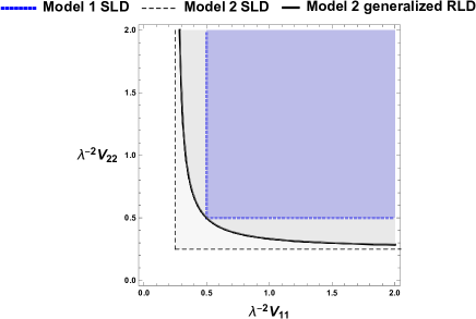
Figure 1: The uncertainty relation of Model 1 and Model 2 given by the inequalities Eqs. (18, 19). The allowed region of Model 2 for the MSE matrix components $(V_{11},\,V_{22})$ is above the solid line, the dark gray region and the blue region given by the inequality (30) which is derived from the generalized RLD Cramér-Rao inequality. The allowed region of Model 2 by the SLD C-R inequality consists of the light gray, dark gray and blue regions. The allowed region of Model 2 by the SLD Cramér-Rao inequality is the blue region.

III.2 Discussion

There are two significant differences between the C-R bounds given by Model 1 and Model 2 even though the unitary transformations of Model 1 and Model 2 make the same shift in the position of the probability density as shown in Eq. (27).

First, the SLD and the generalized RLD C-R bounds of Model 2 is lower than the SLD C-R bound of Model 1. In particular, the SLD C-R bound of Model 2 is a half of that of Model 1. At first sight, this difference in estimation accuracy might puzzle us, since two models displace the same amount in the position. However, there is no inconsistency in our models, and the simple answer is given as follows. Note that the generators for Model 2 shift twice of Model 1 as in Eqs. (9, 11) in the parameter space. This results in the larger quantum Fisher information of Model 2. The measurement accuracy appears to be better in Model 2 only because Model 2 shifts more.

Second, Eq. (30) gives the achievable bound of Model 2 fujiwara2 . The relation between $V_{11}$ and $V_{22}$ in the right hand side of Eq. (30) is not just a product of $V_{11}$ and $V_{22}$ unlike the Heisenberg-Robertson type uncertainty relation. The difference in the bound between Model 1 and Model 2 is caused by the phase shift of Model 2 in Eq. (26). Although this phase shift in Eq. (26) makes no change in the position probability density, it does make a change in the quantum Fisher information matrices.

IV Mixed state model: Effect of thermal noise

Next, we use a mixed state as the reference state to see how the noise affects the measurement accuracy of the electron position. For this purpose, as the mixed state, we choose the thermal state. However, in the current system we are considering, there is no unique thermal state, because the energy eigenstate is degenerated. Then, the thermal state of this system is not uniquely specified by the temperature only. To resolve this degeneracy problem, we impose a condition that the expectation value of the angular momentum $\langle L\rangle_{0}$ is fixed. This is done by introducing a chemical potential.

IV.1 Reference state

Given $\langle L\rangle_{0}$ is fixed at a constant, the reference state $\rho_{\beta,\,\mu}$ is denoted by

$$\rho_{\beta,\,\mu}=Z_{\beta,\,\mu}^{-1}\mathrm{e}^{-\beta H+\mu L},$$ (31)

where $\beta=T^{-1}$ is the inverse temperature and $Z_{\beta,\,\mu}=\mathrm{tr}\,[\exp(-\beta H+\mu L)]$ is the partition function. The parameter $\mu$ is the chemical potential, which will be determined later. The role of the chemical potential $\mu$ is to keep $\langle L\rangle_{0}$ constant to avoid complications by the degeneracy of angular momentum. The use of the chemical potential here is the same idea as seen in the grand canonical ensemble of statistical physics where the chemical potential is used to keep the expectation value of the number of particles constant.

From Eqs. (13, 14),

$$\rho_{\beta,\,\mu}=Z_{\beta,\,\mu}^{-1}\mathrm{e}^{-\frac{1}{2}\beta\omega}\mathrm{e}^{-(\beta\omega-\mu)a^{\dagger}a-\mu b^{\dagger}b}.$$ (32)

By using the Gaussian states which are defined by

$$a\ket{z}_{a}=z\ket{z}_{a},\>\>b\ket{z}_{b}=z\ket{z}_{b},$$ (33)

the reference state $\rho_{\beta,\,\mu}$ is expressed as

$$\rho_{\beta,\,\mu}=\rho_{0,\,a}\otimes\rho_{0,\,b},$$ (34)

where $\rho_{0,\,a}$ and $\rho_{0,\,b}$ are the thermal states with different temperatures. Explicitly, they are

$$\rho_{0,\,a} =\frac{1}{2\pi\kappa_{\mathrm{a}}^{2}}\int\mathrm{e}^{-\frac{|z|^{2}}{2\kappa_{\mathrm{a}}^{2}}}\,|z\rangle_{a}\,{{}_{a}}\langle z\,|\,d^{2}z,$$

$$\rho_{0,\,b} =\frac{1}{2\pi\kappa_{\mathrm{b}}^{2}}\int\mathrm{e}^{-\frac{|z|^{2}}{2\kappa_{\mathrm{b}}^{2}}}\,|z\rangle_{b}\,{{}_{b}}\langle z\,|\,d^{2}z,$$

with

$$2\kappa_{\mathrm{a}}^{2}=(\mathrm{e}^{\beta\omega-\mu}-1)^{-1},\quad 2\kappa_{\mathrm{b}}^{2}=(\mathrm{e}^{\mu}-1)^{-1}.$$ (35)

The derivation of Eqs. (34, 35) is given in A.2. It is straightforward to calculate the expectation value $\langle L\rangle_{0}$ as

$$\langle L\rangle_{0}=\mathrm{tr}\,[L\,\rho_{\beta,\,\mu}]=2\kappa_{\mathrm{a}}^{2}-2\kappa_{\mathrm{b}}^{2}.$$ (36)

From Eqs. (35, 36), we obtain

$$(\langle L\rangle_{0}+1)\mathrm{e}^{2\mu}-\langle L\rangle_{0}(\mathrm{e}^{\,\beta\omega}+1)\mathrm{e}^{\mu}+(\langle L\rangle_{0}-1)\mathrm{e}^{\,\beta\omega}=0.$$ (37)

When $\beta\omega$ and $\langle L\rangle_{0}$ are given, $\mu$ is the variable of Eq. (37). If $\langle L\rangle_{0}=-1$ holds, there exists a unique solution. Whereas there are two solutions for $\langle L\rangle_{0}\neq-1$. However, one of them is shown to be unphysical giving a negative temperature state in the later case. Then, the chemical potential $\mu$ as a function of $\langle L\rangle_{0}$ and $\beta\omega$ is found to be

$$\mathrm{e}^{\mu}=\begin{cases}\displaystyle\frac{2\mathrm{e}^{\,\beta\omega}}{\mathrm{e}^{\,\beta\omega}+1}\hfill(\langle L\rangle_{0}=-1)\\[6.45831pt] \displaystyle\frac{1}{2(\langle L\rangle_{0}+1)}\Big{[}\langle L\rangle_{0}(\mathrm{e}^{\,\beta\omega}+1)+\sqrt{\langle L\rangle_{0}^{2}(\mathrm{e}^{\,\beta\omega}-1)^{2}+4\mathrm{e}^{\,\beta\omega}}\Big{]}\\ \hfill(\langle L\rangle_{0}\neq-1)\end{cases}.$$ (38)

Although the solution of Eq. (37) has a singular point at $\langle L\rangle_{0}=-1$ at a first glance, we can show that the solution the solution for $\langle L\rangle_{0}\neq-1$ is continuously connected to the solution for $\langle L\rangle_{0}=-1$. We can also show that the first derivative is continuous at $\langle L\rangle_{0}=-1$.

Figure 2 shows $\mu$ as a function of $\langle L\rangle_{0}$ at $\beta\omega=0.1,\,1,$ and $5$ from top to bottom. The chemical potential $\mu$ as a function of $\langle L\rangle_{0}$ diverges for $\langle L\rangle_{0}\geq 0$ as $\beta\omega$ goes to infinity, i.e., the zero temperature limit. At a special case, $\langle L\rangle_{0}=0$, we see $\mu=\beta\omega/2$ from Eq. (38). Explicitly, the zero temperature limit is

$$\lim_{\beta\to\infty}\mu=\begin{cases}\infty&\quad(\langle L\rangle_{0}\geq 0)\\[6.45831pt] \log\left[\frac{\langle L\rangle_{0}-1}{\langle L\rangle_{0}}\right]&\quad(\langle L\rangle_{0}<0)\end{cases}.$$ (39)

Figure 2: The chemical potential $\mu$ as a function of the expectation value of the angular momentum $\langle L\rangle_{0}$ at three different temperature parameters $\beta\omega=0.1,\,1$, and $5$. At lower $\beta\omega$ i.e., higher temperature, $\mu$ becomes closer to zero, no preference for the angular momentum.

For Model 2, the two-parameter family of the states $\rho_{\theta}^{\pi}$ is expressed as

$$\rho^{\pi}_{\theta}=\mathrm{e}^{-\mathrm{i}\theta_{1}\pi_{x}}\mathrm{e}^{-\mathrm{i}\theta_{2}\pi_{y}}\rho_{0,\,a}\otimes\rho_{0,\,b}\,\mathrm{e}^{\mathrm{i}\theta_{2}\pi_{y}}\mathrm{e}^{\mathrm{i}\theta_{1}\pi_{x}},$$ (40)

from Eqs. (6, 34). Since $\pi_{x}$ and $\pi_{y}$ consist of $a$ and $a^{\dagger}$ only, $\rho^{\pi}$ is described as

$$\rho^{\pi}_{\theta}=\mathrm{e}^{-\mathrm{i}\theta_{1}\pi_{x}}\mathrm{e}^{-\mathrm{i}\theta_{2}\pi_{y}}\rho_{0,\,a}\,\mathrm{e}^{\mathrm{i}\theta_{2}\pi_{y}}\mathrm{e}^{\mathrm{i}\theta_{1}\pi_{x}}\otimes\rho_{0,\,b}.$$ (41)

Therefore, $\rho_{0,\,b}$ gives no effect to the quantum Fisher information matrices. The reference state $\rho_{\beta,\,\mu}$ for Model 2, we only need to use $\rho_{0,\,a}$. By construction, the family of the states:

$$\rho_{\theta,\,a}=\mathrm{e}^{\xi a^{\dagger}-\xi^{\ast}a}\rho_{0,\,a}\,\mathrm{e}^{\xi^{\ast}a-\xi a^{\dagger}},$$

with $\xi=(2\lambda)^{-1}(\theta_{1}-\mathrm{i}\theta_{2})$, is a Gaussian shift model holevo ; yuen . It is then known that the RLD C-R bound provides the achievable bound holevo ; yuen .

IV.2 Uncertainty relation

For the mixed-state model, we can calculate the SLD and the RLD C-R bounds. They then provide the uncertainty relation for the MSE matrix. The calculations of SLDs and RLDs and their quantum Fisher information matrices are given in B.1.

IV.2.1 Model 1: Unitary model generated by $p_{x}$ and $p_{y}$

Let $G_{\mathrm{R}}^{p\,\mathrm{thermal}}$ and $G_{\mathrm{S}}^{p\,\mathrm{thermal}}$ be the RLD and the SLD Fisher information matrices with respect to $\rho_{\beta,\,\mu}$, respectively. We introduce ${g_{\mathrm{R}}}^{ij}$ and ${g_{\mathrm{S}}}^{ij}$ such that

$$(G_{\mathrm{R}}^{p\,\mathrm{thermal}})^{-1} =[{g_{\mathrm{R}}}^{ij}],$$ (42)

$$(G_{\mathrm{S}}^{p\,\mathrm{thermal}})^{-1} =[{g_{\mathrm{S}}}^{ij}].$$ (43)

The inverse of $G_{\mathrm{R}}^{p\,\mathrm{thermal}}$ is calculated as

$$(G_{\mathrm{R}}^{p\,\mathrm{thermal}})^{-1}=\frac{\lambda^{2}}{1+2\kappa_{\mathrm{a}}^{2}+2\kappa_{\mathrm{b}}^{2}}\begin{pmatrix}2\kappa_{\mathrm{a}}^{2}+2\kappa_{\mathrm{b}}^{2}+8\kappa_{\mathrm{a}}^{2}\kappa_{\mathrm{b}}^{2}&\mathrm{i}\,(2\kappa_{\mathrm{b}}^{2}-2\kappa_{\mathrm{a}}^{2})\\ -\mathrm{i}\,(2\kappa_{\mathrm{b}}^{2}-2\kappa_{\mathrm{a}}^{2})&2\kappa_{\mathrm{a}}^{2}+2\kappa_{\mathrm{b}}^{2}+8\kappa_{\mathrm{a}}^{2}\kappa_{\mathrm{b}}^{2}\\ \end{pmatrix}.$$

From Eq. (19), we have the following inequality,

$$(V_{11}-{g_{\mathrm{R}}}^{11})(V_{22}-{g_{\mathrm{R}}}^{11})\geq\lambda^{4}\left(\frac{2\kappa_{\mathrm{a}}^{2}-2\kappa_{\mathrm{b}}^{2}}{1+2\kappa_{\mathrm{a}}^{2}+2\kappa_{\mathrm{b}}^{2}}\right)^{2}.$$ (44)

Next, the calculation of the inverse of $G_{\mathrm{S}}^{p\,\mathrm{thermal}}$ reveals that $(G_{\mathrm{S}}^{p\,\mathrm{thermal}})^{-1}$ is a diagonal matrix and that ${g_{\mathrm{S}}}^{11}$ is equal to ${g_{\mathrm{S}}}^{22}$. $(G_{\mathrm{S}}^{p\,\mathrm{thermal}})^{-1}$ is written as

$$(G_{\mathrm{S}}^{p\,\mathrm{thermal}})^{-1}=\begin{pmatrix}{g_{\mathrm{S}}}^{11}&0\\ 0&{g_{\mathrm{S}}}^{22}\\ \end{pmatrix},$$ (45)

where

$${g_{\mathrm{S}}}^{11}={g_{\mathrm{S}}}^{22}=\lambda^{2}\frac{\frac{1}{2}+2\kappa_{\mathrm{a}}^{2}+2\kappa_{\mathrm{b}}^{2}+8\kappa_{\mathrm{a}}^{2}\kappa_{\mathrm{b}}^{2}}{1+2\kappa_{\mathrm{a}}^{2}+2\kappa_{\mathrm{b}}^{2}}.$$

From Eq. (18), we have

$$V_{11}\geq{g_{\mathrm{S}}}^{11},\quad V_{22}\geq{g_{\mathrm{S}}}^{11}.$$ (46)

There are two cases regarding the ordering between the inverse of RLD and SLD Fisher matrices in terms of the matrix inequality.

Case i). When $|\langle L\rangle_{0}|\leq 1/2$, the SLD C-R bound defines a tighter lower bound. This is because the matrix inequality

$$(G_{\mathrm{S}}^{p\,\mathrm{thermal}})^{-1}-(G_{\mathrm{R}}^{p\,\mathrm{thermal}})^{-1}=\Delta g\begin{pmatrix}1&-2\mathrm{i}\,\langle L\rangle_{0}\\ 2\mathrm{i}\,\langle L\rangle_{0}&1\\ \end{pmatrix}\geq 0,$$

holds if and only if $|\langle L\rangle_{0}|\leq 1/2$ is satisfied. Here, $\Delta g$ is defined by

$$\Delta g:={g_{\mathrm{S}}}^{11}-{g_{\mathrm{R}}}^{11}=\frac{\lambda^{2}}{2}\frac{1}{1+2\kappa_{\mathrm{a}}^{2}+2\kappa_{\mathrm{b}}^{2}}>0.\\$$ (47)

Case ii). In the other case, $|\langle L\rangle_{0}|>1/2$, however, there is no matrix ordering between the RLD and the SLD Fisher information matrices. This means that both inequalities (44) and (46) contribute to the uncertainty relation. Figure 3 shows an example of the bound given by the current analysis with $|\langle L\rangle_{0}|>1/2$. The parameters used are $\kappa_{\mathrm{a}}^{2}=1,\,\kappa_{\mathrm{b}}^{2}=1/2$, and thus $|\langle L\rangle_{0}|=1>1/2$ holds. The blue region defined by two quantum C-R bounds, the SLD and the RLD C-R bounds are the allowed region of $(V_{11}$, $V_{22})$. The RLD and the SLD C-R bounds have two intersection points in this case. Let the position of one of the intersection points be $(V^{\mathrm{R-S}}_{11},\,{g_{\mathrm{S}}}^{11})$ which is marked as the dot in Fig. 3. The RLD C-R bound defines the bound in the region where ${g_{\mathrm{S}}}^{11}<V_{11}<V^{\mathrm{R-S}}_{11}$. The SLD C-R bound defines in the region where $V_{11}>V^{\mathrm{R-S}}_{11}$ and $V_{22}>V^{\mathrm{R-S}}_{11}$. We define $\Delta V^{\mathrm{R-S}}$ by $\Delta V^{\mathrm{R-S}}=V^{\mathrm{R-S}}_{11}-{g_{\mathrm{S}}}^{11}$. Then, $\Delta V^{\mathrm{R-S}}$ is

$$\Delta V^{\mathrm{R-S}}=\Delta g(4\langle L\rangle_{0}^{2}-1).$$ (48)

Figure 4 shows $\Delta V^{\mathrm{R-S}}$ as a function of $\langle L\rangle_{0}$ at three different $\beta\omega$’s which are the same as Fig. 2.

When $|\langle L\rangle_{0}|\leq 1/2$, $\Delta V^{\mathrm{R-S}}$ is negative as shown in Eq. (48), the RLD C-R bound stays always below the SLD C-R bound. This is consistent with $(G_{\mathrm{S}})^{-1}\geq(G_{\mathrm{R}})^{-1}$ when $|\langle L\rangle_{0}|\leq 1/2$. At larger $\beta\omega$ (lower temperature), the possible ranges of $V^{\mathrm{R-S}}_{11}$ and $V^{\mathrm{R-S}}_{22}$ given by the RLD C-R bound becomes larger at the same $\langle L\rangle_{0}$.

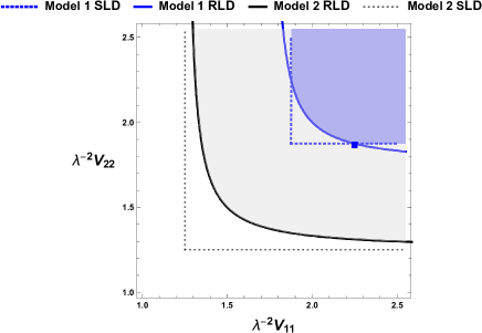
Figure 3: Uncertainty relation of Model 1 and Model 2 given by the quantum Cramér-Rao inequalites. The temperature parameters used are $\,\kappa_{\mathrm{a}}^{2}=1,\,\kappa_{\mathrm{b}}^{2}=1/2,\,\langle L\rangle_{0}=1$, i.e., $\langle L\rangle_{0}>1/2$. The allowed region of Model 1 for the MSE matrix components $(V_{11},\,V_{22})$ is the blue region. The allowed region of Model 1 is given by the SLD Cramér-Rao bound (blue dotted lines) and the RLD C-R bound (blue solid line). The allowed region of Model 2 for the MSE matrix components $(V_{11},\,V_{22})$ is covered by the gray and blue region. The RLD Cramér-Rao bound (black solid line) is achievable. $\Delta V^{\mathrm{R-S}}$ [Eq. (48)] is the distance between the blue square in the figure and the intersection of SLD Cramér-Rao bounds (blue dotted lines).

Figure 4: $\Delta V^{\mathrm{R-S}}$ [Eq. (48)] as a function of $\langle L\rangle_{0}$. By the definition of $\Delta V^{\mathrm{R-S}}$, when $\Delta V^{\mathrm{R-S}}$ is negative, the bound is determined by the SLD Cramér-Rao bound only.

Finally, we briefly discuss achievability of the uncertainty relation above. It is known that the RLD C-R bound is (asymptotically) achievable, if and only when the model is D-invariant suzuki . This condition is checked by comparing two matrices, the inverse of the RLD Fisher information matrix and the $Z$ matrix. As given in B, $(G_{\mathrm{R}}^{p\,\mathrm{thermal}})^{-1}$ and the $Z$ matrix $Z^{p\,\mathrm{thermal}}$ are different. Hence, the RLD C-R bound is not tight. We next examine if the SLD C-R bound is achievable or not. In Refs. RJDD16 ; suzuki18 , the necessary and sufficient conditions are derived for asymptotically achievability of the SLD C-R bound. The simplest condition is that the imaginary part of the $Z$ matrix is zero. In our model, this is equivalent to $\langle L\rangle_{0}=0$ which is also equivalent to $\kappa_{\mathrm{a}}=\kappa_{\mathrm{b}}$ [Eq. (36)]. When $\langle L\rangle_{0}\neq 0$, neither the RLD C-R bound nor SLD C-R bound is even asymptotically achievable. Therefore, the uncertainty relation is not tight, except for the special choice of the parameter, $\langle L\rangle_{0}=0$.

IV.2.2 Model 2 : Unitary model generated by $\pi_{x}$ and $\pi_{y}$

The SLD and the RLD Fisher information matrices of Model 2 are denoted by $G_{\mathrm{S}}^{\pi\,\mathrm{thermal}}$ and $G_{\mathrm{R}}^{\pi\,\mathrm{thermal}}$, respectively. Their inverse matrices $(G_{\mathrm{S}}^{\pi\,\mathrm{thermal}})^{-1}$ and $(G_{\mathrm{R}}^{\pi\,\mathrm{thermal}})^{-1}$ are

$$(G_{\mathrm{S}}^{\pi\,\mathrm{thermal}})^{-1} =\frac{\lambda^{2}}{4}\begin{pmatrix}1+4\kappa_{\mathrm{a}}^{2}&0\\ 0&1+4\kappa_{\mathrm{a}}^{2}\\ \end{pmatrix},$$ (49)

$$(G_{\mathrm{R}}^{\pi\,\mathrm{thermal}})^{-1} =\frac{\lambda^{2}}{4}\begin{pmatrix}1+4\kappa_{\mathrm{a}}^{2}&\mathrm{i}\\ -\mathrm{i}&1+4\kappa_{\mathrm{a}}^{2}\\ \end{pmatrix}.$$ (50)

Since this model is a Gaussian shift model holevo ; yuen , the RLD C-R bound is achievable. By using Eq. (19), the RLD C-R inequality gives the following inequality

$$\left[V_{11}-\frac{\lambda^{2}}{4}(1+4\kappa_{\mathrm{a}}^{2})\right]\left[V_{22}-\frac{\lambda^{2}}{4}(1+4\kappa_{\mathrm{a}}^{2})\right]\geq\frac{\lambda^{4}}{16}.$$ (51)

From Eq. (18), we obtain the SLD C-R bound as follows.

$$V_{11}\geq\frac{\lambda^{2}}{4}(1+4\kappa_{\mathrm{a}}^{2}),\>\>V_{22}\geq\frac{\lambda^{2}}{4}(1+4\kappa_{\mathrm{a}}^{2}).$$

Figure 3 shows the RLD C-R bound and the SLD C-R bound above for the temperature parameter $\kappa_{\mathrm{a}}^{2}=1$ as well. The gray region is the uncertainty relation given by the RLD C-R bound. The SLD and RLD C-R bounds move away from the origin$=(0,0)$ as $\kappa_{\mathrm{a}}^{2}$ increases. This makes sense, because the increase in $\kappa_{\mathrm{a}}^{2}$ means the decrease in $\beta$ because $2\kappa_{\mathrm{a}}^{2}=(\mathrm{e}^{\beta\omega-\mu}-1)^{-1}$. The C-R bounds of Model 2 stays lower than that of Model 1.

IV.3 Discussion

IV.3.1 Mixed state model

It turns out that in the case of the thermal state as the reference state, Model 2 is a simple Gaussian shift model which is known to be the RLD C-R inequality giving an achievable bound holevo ; yuen . However, the bound for Model 1 has a complicated structure as shown in Fig. 3, although the bound for the pure state is simple. As given in A.3, the two-parameter unitary transformation for Model 1, $\mathrm{e}^{-\mathrm{i}\theta_{1}p_{x}}\mathrm{e}^{-\mathrm{i}\theta_{2}p_{y}}$ can be written as

$$\mathrm{e}^{-\mathrm{i}\theta_{1}p_{x}}\mathrm{e}^{-\mathrm{i}\theta_{2}p_{y}}=\mathrm{e}^{\xi_{1}a^{\dagger}-\xi_{1}^{\ast}a}\mathrm{e}^{\xi_{2}^{\ast}b^{\dagger}-\xi_{2}b},$$ (52)

where $\xi_{2}=\xi_{1}^{\ast}$ and $\xi_{1}=(2\lambda)^{-1}(\theta_{1}-\mathrm{i}\theta_{2})$. According to Eq. (52), Model 1 is a two-parameter sub-model with a constraint $\xi_{2}=\xi_{1}^{\ast}$ embedded in the four-parameter model. We attribute this dependency between $\xi_{1}$ and $\xi_{2}$ to the complicated bound though it is not clear why the change in the bound occurs at $\langle L\rangle_{0}=1/2$.

By adding noise with using the mixed state, the thermal state as the reference state changes the feature of the uncertainty relation drastically from the case of the pure state as the reference state. In both cases, Model 2 potentially gives more precise way of estimating the position of the electron than Model 1 does.

IV.3.2 Effects of thermal noise

We next compare the results between the pure state and the thermal state as the reference state as follows. First, Model 1 with the pure state as the reference state, the C-R bound has a quasi-classical feature. The SLD C-R bound is determined by the constant which is the spread of the position probability density of LLL. With the thermal state as the reference state, Model 1 is not D-invariant and the uncertainty relation of Model 1 is complicated. The shape of the C-R bound depends on the expectation value of angular momentum $\langle L\rangle_{0}$. The SLD C-R bound becomes achievable only at $\langle L\rangle_{0}=0$. Unless this special condition is satisfied, the mixed state model with the thermal noise has discontinuity from zero temperature to finite temperature in the quantum C-R bounds. And hence, we cannot simply take the zero temperature limit from the thermal state in our model.

Next, Model 2 with the pure state as the reference state, the generalized RLD exists. The C-R bound given by the generalized RLD is achievable. The MSE matrix components $V_{11}$ and $V_{22}$ has a correlation as shown in Eq. (30). With the thermal state as the reference state, Model 2 is a simple Gaussian shift model. Unlike the case of Model 1, Model 2 with the pure state as the reference state is genuine quantum. For Model 2, there exists a limit when the temperature goes to zero, or equivalently, $\beta\to\infty$ fujiwara2 . This limit yields the result for the pure-state case studied in Sec. III.1.2.

IV.3.3 Optical implementation

The models studied in this paper can naturally be realized in the two-dimensional electron gas at low temperature. However, the optimal measurement to attain the quantum C-R bound may not be feasible in such a system. Alternatively, one can realize our models in a linear optical system with two modes by tuning parameters properly. In this connection, we should not forget to mention related works on parameter estimation problems in two mode Gaussian states Refs. CI01 ; Gal13 ; GL14 ; BD16 ; BAL17 ; BLA18 ; AKC19 . In Ref. AKC19 , authors discussed an optimal encoding and measurement scheme for estimating two parameters in the pure-state reference state. The optimal state found there also comprises of classical correlation of the phase conjugation as in Eq. (52) for Model 1. The optimal POVM for Model 2 requires measuring non-canonical variables. $\pi_{x}$ and $\pi_{y}$ aharonov . Therefore, we can only state that Model 2 potentially gives more precise measurement. We expect that our result in the thermal state as a reference state should also relevant to finding the optimal scheme in the presence of noise.

V Conclusion

We have investigated the uncertainty relation for estimating $x$ and $y$ components of the position of one electron in a uniform magnetic field. In the present study, the uncertainty relation upon estimating the expectation values of the two commuting observables, $(x,\,y)$ was derived in the framework of the quantum estimation theory. As the generators of the unitary transformation, two different sets of generators are used. One is a set of canonical momenta, $p_{x}$ and $p_{y}$ (Model 1) and the other is a set of mechanical momenta, $\pi_{x}$ and $\pi_{y}$ (Model 2). Based on the analysis by the quantum estimation theory, in both cases, we got non-trivial bounds that give the trade-off relations between the two commuting observables, $x$ and $y$, unlike the result of Heisenberg-Robertson type uncertainty relation.

Although both Model 1 and Model 2 give the same effect to the position probability density defined by the product of the wave function and its complex conjugate, the C-R bounds of Model 1 and Model 2 are different for pure state and mixed state (thermal state) as the reference state.

With the pure state as the reference state, the C-R bound is quasi-classical for Model 1 and it is quantum mechanical for Model 2. With the thermal state as the reference state, the uncertainty relation given by the C-R bounds is complicated and the shape of the bounds changes when the expectation value of the angular momentum $\langle L\rangle_{0}$ is equal to $1/2$ for Model 1. Model 2 becomes a simple Gaussian shift model. In either case of the pure or thermal state, Model 2 potentially gives more precise measurement.

Before closing this paper, we make two remarks. First, the C-R bound of Model 1 with respect to the thermal state reference state is not achievable except for $\langle L\rangle_{0}=0$. A possible extension might be an analysis by minimizing a weighted trace of the mean square error matrix kull . However, this method gives asymptotically achievable bound only. Second, for the thermal state with the $\langle L\rangle_{0}$ constraint, we see the change in the bound shape depending on $\langle L\rangle_{0}$. We have no clue as to why the bound shape changes at $\langle L\rangle_{0}=1/2$ in a simple physical picture so far. It should be worthwhile seeing why the bound shape changes there.

Appendix A Supplement

A.1 Uncertainty relation by quantum C-R inequality

The quantum C-R inequality for the MSE matrix $V_{\theta}$ is

$$V_{\theta}\geq(G_{\theta})^{-1},$$ (53)

where $G_{\theta}$ is an arbitrary quantum Fisher information matrix. Let $(G_{\theta})^{-1}$ be

$$(G_{\theta})^{-1}=[{g_{\theta}}^{ij}],$$ (54)

The RLD C-R inequality (53) holds iff $\mathrm{tr}\,[V_{\theta}-(G_{\theta})^{-1}]\geq 0$ and $\mathrm{det}\,[V_{\theta}-(G_{\theta})^{-1}]\geq 0$. Thus, we have

$$V_{\,11}-{g_{\theta}}^{11}\geq 0,\quad V_{\,22}-{g_{\theta}}^{22}\geq 0,$$

and

$$\mathrm{det}\begin{pmatrix}V_{11}-{g_{\theta}}^{11}&V_{12}-{g_{\theta}}^{12}\\ V_{21}-({g_{\theta}}^{12})^{\ast}&V_{22}-{g_{\theta}}^{22}\\ \end{pmatrix}\geq 0,$$

where $g_{\theta}^{21}=(g_{\theta}^{12})^{\ast}$ is used. The inequality above gives the following inequality.

$$(V_{11}-{g_{\theta}}^{11})(V_{22}-{g_{\theta}}^{22})\geq|V_{12}-{g_{\theta}}^{12}\,|^{2}.$$

The right hand side of the inequality above is written as follows.

$$|V_{12}-{g_{\theta}}^{12}\,|^{2} =|V_{12}-\mathrm{Re}\,{g_{\theta}}^{12}-\mathrm{i}\,\mathrm{Im}\,{g_{\theta}}^{12}\,|^{2}$$

$$=|V_{12}-\mathrm{Re}\,{g_{\theta}}^{12}\,|^{2}+|\,\mathrm{Im}\,{g_{\theta}}^{12}\,|^{2}$$

$$\geq|\,\mathrm{Im}\,{g_{\theta}}^{12}\,|^{2}.$$

By applying this inequality, we obtain the following inequalities,

$$V_{11}-{g_{\theta}}^{11}\geq 0,\quad V_{\,22}-{g_{\theta}}^{22}\geq 0,$$ (55)

$$(V_{11}-{g_{\theta}}^{11})(V_{22}-{g_{\theta}}^{22})\geq|\,\mathrm{Im}\,{g_{\theta}}^{12}\,|^{2}.$$ (56)

When $\mathrm{Im}\,{g_{\theta}}^{12}=0$, the uncertainty relation is given by Eq. (55) only.

A.2 Thermal state and Gaussian state

The thermal state for a single harmonic oscillator, $\rho_{\beta}$ is described as

$$\rho_{\beta}=Z_{\beta}^{-1}\mathrm{e}^{-\beta H},$$ (57)

where $Z_{\beta}=\mathrm{tr}\,[\mathrm{e}^{-\beta H}]$ and $\beta=T^{-1}$. $T$ is temperature.

By using Hamiltonian $H=\omega\,(a^{\dagger}a+1/2)$ and $a^{\dagger}a\ket{n}=n\ket{n}$, $\,\mathrm{e}^{-\beta H}$ is

$$\mathrm{e}^{-\beta H}=\sum_{n=0}^{\infty}\mathrm{e}^{-\beta H}\ket{n}\bra{n}\\ =\mathrm{e}^{-\frac{1}{2}\beta\omega}\sum_{n=0}^{\infty}\gamma^{n}\ket{n}\bra{n},$$

where $\gamma=\mathrm{e}^{-\beta\omega}$. $Z_{\beta}$ is

$$Z_{\beta}=\mathrm{tr}\,[\mathrm{e}^{-\beta H}]\\ =\frac{\mathrm{e}^{-\frac{1}{2}\beta\omega}}{1-\gamma}.$$

We obtain

$$\rho_{\beta}=Z_{\beta}^{-1}\mathrm{e}^{-\beta H}=(1-\gamma)\sum_{n}\gamma^{n}\ket{n}\bra{n}.$$

We first calculate the matrix element of $\rho_{\beta}$ by the basis as the Gaussian state, $\braket{z_{1}}{\rho_{\beta}}{z_{2}}$. Next, we make the same matrix element of the Gaussian state to see if they match.

$\braket{z_{1}}{\rho_{\beta}}{z_{2}}$ is

$$\braket{z_{1}}{\rho_{\beta}}{z_{2}} =(1-\gamma)\sum_{n}\gamma^{n}\braket{z_{1}}{n}\braket{n}{z_{2}}$$

$$=(1-\gamma)\mathrm{e}^{-\frac{1}{2}|z_{1}|^{2}-\frac{1}{2}|z_{2}|^{2}+\gamma z_{1}^{\ast}z_{2}}.$$ (58)

The Gaussian state $S_{\kappa}$ is defined by

$$S_{\kappa}=\frac{1}{2\pi\kappa^{2}}\int\mathrm{e}^{-\frac{|z|^{2}}{2\kappa^{2}}}\ket{z}\bra{z}d^{2}z.$$

Then its matrix element $\bra{z_{1}}S_{\kappa}\ket{z_{2}}$ is

$$\bra{z_{1}}S_{\kappa}\ket{z_{2}} =\frac{1}{2\pi\kappa^{2}}\int\mathrm{e}^{-\frac{|z|^{2}}{2\kappa^{2}}}\braket{z_{1}}{z}\braket{z}{z_{2}}d^{2}z$$

$$=\frac{1}{2\pi\kappa^{2}}\int\mathrm{e}^{-(\frac{1}{2\kappa^{2}}+1)|z|^{2}+z_{1}^{\ast}z_{2}+z_{1}z_{2}^{\ast}}d^{2}z\,\mathrm{e}^{-\frac{1}{2}|z_{1}|^{2}-\frac{1}{2}|z_{2}|^{2}}.$$

By using

$$\int\mathrm{e}^{-\alpha|z|^{2}+\beta z+\gamma z^{\ast}}d^{2}z=\frac{\pi}{\alpha}\mathrm{e}^{\frac{\beta\gamma}{\alpha}},$$

we obtain

$$\bra{z_{1}}\rho_{\beta}\ket{z_{2}}=\frac{1}{2\kappa^{2}+1}\mathrm{e}^{-\frac{1}{2}|z_{1}|^{2}-\frac{1}{2}|z_{2}|^{2}+\frac{z_{1}^{\ast}z_{2}}{\frac{1}{2\kappa^{2}}+1}}.$$ (59)

From (58) and (59), $\braket{z_{1}}{S_{\kappa}}{z_{2}}=\bra{z_{1}}\rho_{\beta}\ket{z_{2}}$ holds iff

$$2\kappa^{2}=\dfrac{\gamma}{1-\gamma}=\frac{1}{\mathrm{e}^{\beta\omega}-1}.$$ (60)

Therefore, we obtain

$$\rho_{\beta}=\frac{1}{2\pi\kappa^{2}}\int\mathrm{e}^{-\frac{|z^{\prime}|^{2}}{2\kappa^{2}}}\ket{z}\bra{z}d^{2}z.$$ (61)

where $2\kappa^{2}$ is given by Eq. (60).

A.3 Model 1 unitary transformation
in terms of the creation and annihilation operators

The unitary transformations of the Model 1, $\mathrm{e}^{-\mathrm{i}\theta_{1}p_{x}}\mathrm{e}^{-\mathrm{i}\theta_{2}p_{y}}$ is

$$\mathrm{e}^{-\mathrm{i}\theta_{1}p_{x}}\mathrm{e}^{-\mathrm{i}\theta_{2}p_{y}}=\mathrm{e}^{\frac{1}{2\lambda}\,\{(a^{\dagger}-a)+(b^{\dagger}-b)\}\theta_{1}}\mathrm{e}^{-\frac{\mathrm{i}}{2\lambda}\,\{(a^{\dagger}+a)-(b^{\dagger}+b)\}\theta_{2}}.$$

Since $p_{x}$ and $p_{y}$ commute,

$$\mathrm{e}^{-\mathrm{i}\theta_{1}p_{x}}\mathrm{e}^{-\mathrm{i}\theta_{2}p_{y}}=\mathrm{e}^{-\mathrm{i}\theta_{1}p_{x}-\mathrm{i}\theta_{2}p_{y}}=\mathrm{e}^{\frac{1}{2\lambda}\,\{(a^{\dagger}-a)+(b^{\dagger}-b)\}\theta_{1}\}-\frac{\mathrm{i}}{2\lambda}\,\{(a^{\dagger}+a)-(b^{\dagger}+b)\}\theta_{2}}.$$

Therefore,

$$\mathrm{e}^{-\mathrm{i}\theta_{1}p_{x}}\mathrm{e}^{-\mathrm{i}\theta_{2}p_{y}}=\mathrm{e}^{\xi a^{\dagger}-\xi^{\ast}a}\mathrm{e}^{\xi^{\ast}b^{\dagger}-\xi b},$$ (62)

where $\xi=(2\lambda)^{-1}(\theta_{1}-\mathrm{i}\theta_{2})$.

Appendix B Calculation

B.1 SLD and RLD: The thermal state as the reference state

First, we briefly explain that SLD and RLD Fisher information matrices for the mixed state are independent of the parameters $\theta=(\theta_{1},\,\theta_{2})$ in the unitary transformation $U(\theta_{1},\,\theta_{2})$.

Let Model 1 SLD and Model 1 RLD of Model 1 be $L^{(1)}_{\mathrm{S},\,j}(\theta)$ and $L^{(1)}_{R,\,j}(\theta)$, respectively. With using the unitary transformation $U(\theta_{1},\,\theta_{2})=\mathrm{e}^{-\mathrm{i}\theta_{1}p_{x}}\mathrm{e}^{-\mathrm{i}\theta_{2}p_{y}}$, $L^{(1)}_{\mathrm{S},\,j}(0)$ and $L^{(1)}_{\mathrm{R},\,j}(0)$ are written as

$$L^{(1)}_{\mathrm{S},\,j}(\theta) =U(\theta_{1},\,\theta_{2})\,L^{(1)}_{\mathrm{S},\,j}(0)\,U^{\dagger}(\theta_{1},\,\theta_{2}),$$

$$L^{(1)}_{\mathrm{R},\,j}(\theta) =U(\theta_{1},\,\theta_{2})\,L^{(1)}_{\mathrm{R},\,j}(0)\,U^{\dagger}(\theta_{1},\,\theta_{2}).$$

For the RLD Fisher information $G^{(1)}_{\mathrm{R}}(\theta)=[g^{(1)}_{\mathrm{R},\>ij}(\theta)]$, we can derive the relation below if the transformation is unitary.

$$g^{(1)}_{\mathrm{R},\>ij}(\theta)=\mathrm{tr}\,[\rho_{\theta}\,L^{(1)}_{\mathrm{R},\,j}(\theta)L^{(1)\,\dagger}_{\mathrm{R},\,i}(\theta)]=\mathrm{tr}\,[\rho_{0}\,L_{\mathrm{R},\,j}(0)L^{(1)\,\dagger}_{\mathrm{R},\,i}(0)].$$

If the transformation is unitary, the RLD Fisher information $G_{\mathrm{R}}(\theta)$ does not depend on the parameters $\theta_{1}$ and $\theta_{2}$. Then, we can write $G_{\mathrm{R}}(\theta)$ as $G_{\mathrm{R}}=[g_{\mathrm{R},\>ij}]$. From Eqs. (20,  II.5.2), we can show that the same holds for the SLD Fisher information $G_{\mathrm{S}}(\theta)$. Therefore, if we have $L^{(1)}_{\mathrm{S},\,i}(0)$ and $L^{(1)}_{\mathrm{R},\,i}(0)$, it is enough to obtain the SLD and RLD Fisher information matrices. The same is true for Model 2.

B.1.1 Model 1 SLD: $L^{(1)}_{S,\,1}(0),\,L^{(1)}_{S,\,2}(0),Z\>matrix\>Z^{p\,\mathrm{thermal}}$

$$L^{(1)}_{\mathrm{S},\,1}(0) =\frac{1}{\lambda(1+4\kappa_{\mathrm{a}}^{2})}(a+a^{\dagger})+\frac{1}{\lambda(1+4\kappa_{\mathrm{b}}^{2})}(b+b^{\dagger}),$$

$$L^{(1)}_{\mathrm{S},\,2}(0) =\frac{\mathrm{i}}{\lambda(1+4\kappa_{\mathrm{a}}^{2})}(a-a^{\dagger})-\frac{\mathrm{i}}{\lambda(1+4\kappa_{\mathrm{b}}^{2})}(b-b^{\dagger}).$$

With using $p_{x},\,p_{y}$ and $x,\,y$,

$$L^{(1)}_{\mathrm{S},\,1}(0) =(\frac{1}{1+4\kappa_{\mathrm{a}}^{2}}+\frac{1}{1+4\kappa_{\mathrm{b}}^{2}})p_{y}+\frac{1}{\lambda^{2}}(\frac{1}{1+4\kappa_{\mathrm{a}}^{2}}-\frac{1}{1+4\kappa_{\mathrm{b}}^{2}})\,x,$$

$$L^{(1)}_{\mathrm{S},\,2}(0) =-(\frac{1}{1+4\kappa_{\mathrm{a}}^{2}}-\frac{1}{1+4\kappa_{\mathrm{b}}^{2}})p_{x}+\frac{1}{\lambda^{2}}(\frac{1}{1+4\kappa_{\mathrm{a}}^{2}}+\frac{1}{1+4\kappa_{\mathrm{b}}^{2}})\,y.$$

The SLD Fisher information matrix $G_{\mathrm{S}}^{p\,\mathrm{thermal}}$ is calculated as

$$G_{\mathrm{S}}^{p\,\mathrm{thermal}}=\frac{1}{\lambda^{2}}(\frac{1}{1+4\kappa_{a}^{2}}+\frac{1}{1+4\kappa_{b}^{2}})\begin{pmatrix}1&0\\ 0&1\\ \end{pmatrix}.$$

Z matrix $Z^{p\,\mathrm{thermal}}$ is calculated as

$$Z^{p\,\mathrm{thermal}}=\frac{\lambda^{2}}{1+2\kappa_{\mathrm{a}}^{2}+2\kappa_{\mathrm{b}}^{2}}\begin{pmatrix}\frac{1}{2}+2\kappa_{\mathrm{a}}^{2}+2\kappa_{\mathrm{b}}^{2}+8\kappa_{\mathrm{a}}^{2}\kappa_{\mathrm{b}}^{2}&\mathrm{i}\,(2\kappa_{\mathrm{b}}^{2}-2\kappa_{\mathrm{a}}^{2})\\ -\mathrm{i}\,(2\kappa_{\mathrm{b}}^{2}-2\kappa_{\mathrm{a}}^{2})&\frac{1}{2}+2\kappa_{\mathrm{a}}^{2}+2\kappa_{\mathrm{b}}^{2}+8\kappa_{\mathrm{a}}^{2}\kappa_{\mathrm{b}}^{2}\\ \end{pmatrix}.$$

From this expression, we have

$$Z^{p\,\mathrm{thermal}}=(G_{\mathrm{R}}^{p\,\mathrm{thermal}})^{-1}+\Delta g\begin{pmatrix}1&0\\ 0&1\\ \end{pmatrix}.$$

Since $\Delta g\neq 0$, we see that $Z^{p\,\mathrm{thermal}}\neq(G_{\mathrm{R}}^{p\,\mathrm{thermal}})^{-1}$. This implies the model is not D-invariant suzuki .

B.1.2 Model 2 SLD: $L^{(2)}_{\mathrm{S},\,1}(0),\,L^{(2)}_{\mathrm{S},\,2}(0),Z\>matrix\>Z^{\pi\,\mathrm{thermal}}$

$$L^{(2)}_{\mathrm{S},\,1}(0) =\frac{2}{\lambda(1+4\kappa_{\mathrm{a}}^{2})}(a+a^{\dagger}),$$

$$L^{(2)}_{\mathrm{S},\,2}(0) =\frac{2\mathrm{i}}{\lambda(1+4\kappa_{\mathrm{a}}^{2})}(a-a^{\dagger}).$$

With using $p_{x},\,p_{y}$ and $x,\,y$,

$$L^{(2)}_{\mathrm{S},\,1}(0) =\frac{2}{1+4\kappa_{\mathrm{a}}^{2}}(p_{y}+\frac{1}{\lambda^{2}}x),$$

$$L^{(2)}_{\mathrm{S},\,2}(0) =\frac{2}{1+4\kappa_{\mathrm{a}}^{2}}(-p_{x}+\frac{1}{\lambda^{2}}y).$$

The inverse of the SLD Fisher information matrix $G_{\mathrm{S}}^{\pi\,\mathrm{thermal}}$ is

$$G_{\mathrm{S}}^{\pi\,\mathrm{thermal}}=\frac{4}{\lambda^{2}(1+4\kappa_{\mathrm{a}}^{2})}\begin{pmatrix}1&0\\ 0&1\\ \end{pmatrix}.$$

Z matrix $Z^{\pi\,\mathrm{thermal}}$ is

$$Z^{\pi\,\mathrm{thermal}}=\frac{\lambda^{2}}{4}\begin{pmatrix}1+4\kappa_{\mathrm{a}}^{2}&\mathrm{i}\\ -\mathrm{i}&1+4\kappa_{\mathrm{a}}^{2}\\ \end{pmatrix}.$$

B.1.3 Model 1 RLD: $L^{(1)}_{\mathrm{R},\,1}(0),\,L^{(1)}_{\mathrm{R},\,2}(0)$

$$L^{(1)}_{\mathrm{R},\,1}(0) =\frac{1}{2\lambda}(\frac{1}{1+2\kappa_{\mathrm{a}}^{2}}a+\frac{1}{2\kappa_{\mathrm{a}}^{2}}a^{\dagger})+\frac{1}{2\lambda}(\frac{1}{1+2\kappa_{\mathrm{b}}^{2}}b+\frac{1}{2\kappa_{\mathrm{b}}^{2}}b^{\dagger}),$$

$$L^{(1)}_{\mathrm{R},\,2}(0) =-\frac{\mathrm{i}}{2\lambda}(-\frac{1}{1+2\kappa_{\mathrm{a}}^{2}}a+\frac{1}{2\kappa_{\mathrm{a}}^{2}}a^{\dagger})+\frac{\mathrm{i}}{2\lambda}(-\frac{1}{1+2\kappa_{\mathrm{b}}^{2}}b+\frac{1}{2\kappa_{\mathrm{b}}^{2}}b^{\dagger}).$$

The RLD Fisher information matrix $G_{\mathrm{R}}^{p\,\mathrm{thermal}}$ is calculated as

$$G_{\mathrm{R}}^{p\,\mathrm{thermal}}=\frac{1}{4\lambda^{2}}\begin{pmatrix}\frac{1}{1+2\kappa_{a}^{2}}+\frac{1}{2\kappa_{a}^{2}}+\frac{1}{1+2\kappa_{b}^{2}}+\frac{1}{2\kappa_{b}^{2}}&-\mathrm{i}\,[\frac{1}{2\kappa_{a}^{2}(1+2\kappa_{a}^{2})}-\frac{1}{2\kappa_{b}^{2}(1+2\kappa_{b}^{2})}]\\ \mathrm{i}\,[\frac{1}{2\kappa_{a}^{2}(1+2\kappa_{a}^{2})}-\frac{1}{2\kappa_{b}^{2}(1+2\kappa_{b}^{2})}]&\frac{1}{1+2\kappa_{a}^{2}}+\frac{1}{2\kappa_{a}^{2}}+\frac{1}{1+2\kappa_{b}^{2}}+\frac{1}{2\kappa_{b}^{2}}\end{pmatrix}.$$

B.1.4 Model 2 RLD: $L^{(2)}_{\mathrm{R},\,1}(0),\,L^{(2)}_{\mathrm{R},\,2}(0)$

$$L^{(2)}_{\mathrm{R},\,1}(0) =\frac{1}{\lambda}(\frac{1}{1+2\kappa_{\mathrm{a}}^{2}}a+\frac{1}{2\kappa_{\mathrm{a}}^{2}}a^{\dagger}),$$

$$L^{(2)}_{\mathrm{R},\,2}(0) =\frac{\mathrm{i}}{\lambda}(\frac{1}{1+2\kappa_{\mathrm{a}}^{2}}a-\frac{1}{2\kappa_{\mathrm{a}}^{2}}a^{\dagger}).$$

The creation annihilation operators, $a,\,a^{\dagger}$ and $b,\,b^{\dagger}$ are written as follows.

$$a =\frac{\lambda}{2}[(\mathrm{i}p_{x}+p_{y})+\frac{1}{\lambda^{2}}(x-\mathrm{i}y)],$$

$$a^{\dagger} =\frac{\lambda}{2}[(-\mathrm{i}p_{x}+p_{y})+\frac{1}{\lambda^{2}}(x+\mathrm{i}y)],$$

$$b =\frac{\lambda}{2}[(\mathrm{i}p_{x}-p_{y})+\frac{1}{\lambda^{2}}(x+\mathrm{i}y)],$$

$$b^{\dagger} =\frac{\lambda}{2}[(-\mathrm{i}p_{x}-p_{y})+\frac{1}{\lambda^{2}}(x-\mathrm{i}y)].$$

The RLD Fisher information matrix $G_{\mathrm{R}}^{\pi\,\mathrm{thermal}}$ is

$$G_{\mathrm{R}}^{\pi\,\mathrm{thermal}}=\frac{1}{\lambda^{2}}\frac{1}{2\kappa_{\mathrm{a}}^{2}(1+2\kappa_{\mathrm{a}}^{2})}\begin{pmatrix}1+4\kappa_{\mathrm{a}}^{2}&-\mathrm{i}\\ \mathrm{i}&1+4\kappa_{\mathrm{a}}^{2}\\ \end{pmatrix}.$$

B.2 SLD, Generalized RLD: Pure state as the reference state

Let the SLD of a pure state $\rho_{\theta}=\ket{\psi_{\theta}}\bra{\psi_{\theta}}$ be $L_{S,\,i}$. Then, $L_{\mathrm{S},\,i}$ is expressed as fujiwara2 ,

$$L_{\mathrm{S},\,i}=2{\partial_{i}}\rho_{\theta}=2\partial_{i}(\ket{\psi_{\theta}}\bra{\psi_{\theta}}).$$ (63)

B.2.1 Model 1 SLD: $L^{(1)}_{\mathrm{S},\,1}(\theta),\>L^{(1)}_{\mathrm{S},\,2}(\theta)$

We set the reference state $\rho_{0}$ as $\rho_{0}=\ket{0,\,0}\bra{0,\,0}$. From Eq. (6), $\rho^{p}_{\theta}$ is expressed as

$$\rho^{p}_{\theta} =\mathrm{e}^{-\mathrm{i}\theta_{1}p_{x}}\mathrm{e}^{-\mathrm{i}\theta_{2}p_{y}}\ket{0,\,0}\bra{0,\,0}\mathrm{e}^{\mathrm{i}\theta_{2}p_{y}}\mathrm{e}^{\mathrm{i}\theta_{1}p_{x}}$$ (64)

$$=U(\theta)\ket{0,\,0}\bra{0,\,0}U^{\dagger}(\theta).$$ (65)

where $U(\theta)=\mathrm{e}^{-\mathrm{i}\theta_{1}p_{x}}\mathrm{e}^{-\mathrm{i}\theta_{2}p_{y}}$. From Eq. (63), the SLD’s of Model 1 are expressed as

$$L^{(1)}_{\mathrm{S},\,1}(0) =-2\mathrm{i}[p_{x},\,\rho_{0}],$$

$$L^{(1)}_{\mathrm{S},\,2}(0) =-2\mathrm{i}[p_{y},\,\rho_{0}].$$

where $L^{(1)}_{\mathrm{S},\,j}(\theta)=U(\theta)L^{(1)}_{\mathrm{S},\,j}(0)U^{\dagger}(\theta),\>(j=1,\,2)$.

By using Eq. (9), $L^{(1)}_{S,\,1}(0)$ and $L^{(1)}_{\mathrm{S},\,2}(0)$ are also written as

$$L^{(1)}_{\mathrm{S},\,1}(0) =\frac{1}{\lambda}[(a^{\dagger}-a)+(b^{\dagger}-b),\,\rho_{0}],$$

$$L^{(1)}_{\mathrm{S},\,2}(0) =-\frac{\mathrm{i}}{\lambda}[(a^{\dagger}+a)-(b^{\dagger}+b),\,\rho_{0}].$$

With these SLD’s, the Fisher information matrix $G_{\mathrm{S}}^{p}$ is calculated as

$$G_{\mathrm{S}}^{p}=\frac{2}{\lambda^{2}}\begin{pmatrix}1&0\\ 0&1\\ \end{pmatrix}.$$

From the direct calculation of Eq. (22), we can show that $G_{\mathrm{S}}^{p}=\tilde{G}_{\mathrm{R}}^{p}$.

B.2.2 Model 2 SLD: $L^{(2)}_{\mathrm{S},\,1}(\theta),\>L^{(2)}_{\mathrm{S},\,2}(\theta)$

From Eq. (6), $\rho^{\pi}_{\theta}$ is expressed as

$$\rho^{\pi}_{\theta}=\mathrm{e}^{-\mathrm{i}\theta_{1}\pi_{x}}\mathrm{e}^{-\mathrm{i}\theta_{2}\pi_{y}}\ket{0,\,0}\bra{0,\,0}\mathrm{e}^{\mathrm{i}\theta_{2}\pi_{y}}\mathrm{e}^{\mathrm{i}\theta_{1}\pi_{x}}.$$ (66)

The unitary transformation $\mathrm{e}^{-\mathrm{i}\theta_{1}\pi_{x}}\mathrm{e}^{-\mathrm{i}\theta_{2}\pi_{y}}$ is calculated as follows klauder .

$$\mathrm{e}^{-\mathrm{i}\theta_{1}\pi_{x}}\mathrm{e}^{-\mathrm{i}\theta_{2}\pi_{y}}=\mathrm{e}^{\frac{1}{\lambda^{2}}\theta_{1}\theta_{2}}\mathrm{e}^{-\mathrm{i}\theta_{1}\pi_{x}-\mathrm{i}\theta_{2}\pi_{y}}.$$ (67)

By substituting Eq. (67) in Eq (66), we obtain

$$\rho^{\pi}_{\theta}=U(\theta)\ket{0,\,0}\bra{0,\,0}U^{\dagger}(\theta).$$ (68)

where $U(\theta)=\mathrm{e}^{-\mathrm{i}\theta_{1}\pi_{x}-\mathrm{i}\theta_{2}\pi_{y}}$.

From Eq. (63), the SLD’s of Model 2 are expressed as

$$L^{(2)}_{\mathrm{S},\,1}(0) =-2\mathrm{i}[\pi_{x},\,\rho_{0}],$$

$$L^{(2)}_{\mathrm{S},\,2}(0) =-2\mathrm{i}[\pi_{y},\,\rho_{0}].$$

where $L^{(2)}_{\mathrm{S},\,j}(\theta)=U(\theta)L^{(2)}_{S,\,j}(0)U^{\dagger}(\theta),\>(j=1,\,2)$.

By using Eq. (11),

$$L^{(2)}_{\mathrm{S},\,1}(0) =-\frac{2\mathrm{i}}{\lambda}[a^{\dagger}+a,\,\rho_{0}],$$

$$L^{(2)}_{\mathrm{S},\,2}(0) =\frac{2}{\lambda}[a^{\dagger}-a,\,\rho_{0}].$$

Thus, the SLD Fisher information $G_{\mathrm{S}}^{\pi}$ is

$$G_{\mathrm{S}}^{\pi}=\frac{4}{\lambda^{2}}\begin{pmatrix}1&0\\ 0&1\\ \end{pmatrix}.$$

From Eq. (63), the generalized RLD Fisher information $\tilde{G}_{\mathrm{R}}^{\pi}$ is

$$\tilde{G}_{\mathrm{R}}^{\pi}=\frac{4}{\lambda^{2}}\begin{pmatrix}1&\mathrm{i}\\ -\mathrm{i}&1\\ \end{pmatrix}.$$

References

- (1) C. W. Helstrom Quantum Detection and Estimation Theory, Academic, New York (1976).
- (2) A. S. Holevo, Probabilistic and Statistical Aspects of Quantum Theory, Edizioni della Normale, Pisa, 2nd ed (2011).
- (3) S.L. Braunstein, C. M. Caves, G. J. Milburn, Annals of Physics, 247(1), 135-173 (1996). https://doi.org/10.1006/aphy.1996.0040
- (4) H. Nagaoka, in Surikagaku, no. 508, p. 26–34, Saiense-Sha (2005). (in Japanese)
- (5) P. Gibilisco, H. Hiai, D. Petz, IEEE Trans. Information Theory. A, Vol. 55, 439 (2009). https://doi.org/10.1109/TIT.2008.2008142
- (6) Y. Watanabe, T. Sagawa, M. Ueda, Phys. Rev. A, Vol. 81, 042121 (2011). https://doi.org/10.1103/PhysRevA.84.042121
- (7) W. Guo, W. Zhong, X-X.Jing, L-B. Fu, and X. Wang, Phys. Rev. A, Vol. 93, 042115 (2016). https://link.aps.org/doi/10.1103/PhysRevA.93.042115
- (8) I. Kull, P. Allard Guérin, F. Verstraete, Journal of Physics A: Mathematical and Theoretical, (2020) (forthcoming). https://doi.org/10.1088/1751-8121/ab7f67
- (9) L. I. Mandel’shtam and I. E. Tamm, Izv. AN SSSR ser. fiz. 9, 122 (1945). I. Tamm, J. Phys. (U.S.S.R.) 9, 249 (1945).
- (10) M. Ozawa, Phys. Rev. A, Vol. 67, 042105 (2003). https://doi.org/10.1103/PhysRevA.67.042105
- (11) M. Ozawa, Phys. Lett. A, Vol. 320, 367 (2004). https://doi.org/10.1016/j.physleta.2003.12.001
- (12) S. Wehner and A. Winter J. Math. Phys., Vol. 49, 062105 (2008). https://doi.org/10.1063/1.2943685
- (13) M.G.A Paris, Int. J. Quantum Inf. 7, 125 (2009).
- (14) F. Albarelli, M. Barbieri, M.G. Genoni, I Gianani. Physics Letters A, 384(12), 126311 (2020). https://doi.org/10.1016/j.physleta.2020.126311
- (15) J. S. Sidhu, P. Kok, AVS Quantum Science, 2(1), 014701, (2020). https://doi.org/10.1116/1.5119961
- (16) R. Demkowicz-Dobrzan, W. Gorecki, M. Guta, (2020). arXiv:2001.11742. http://arxiv.org/abs/2001.11742
- (17) W. Heisenberg, Zeitschr. Phys. Vol. 43, 172 (1927). http://dx.doi.org/10.1007/BF01397280
- (18) H. P. Robertson, Phys. Rev. Vol. 34, 163 (1929). https://doi.org/10.1103/PhysRev.34.163
- (19) M. Johnson and B. Lippmann, Phys. Rev, Vol. 76, 828 (1949). https://doi.org/10.1103/PhysRev.76.828
- (20) L. D. Landau and E. M. Lifshitz, Quantum Mechanics (Nonrelativistic Theory), Pergamon, New York, (1977).
- (21) A. Fujiwara, H. Nagaoka J. Math. Phys., Vol. 40, 4227 (1999). https://doi.org/10.1063/1.532962
- (22) A. Fujiwara ”Multiparameter pure state estimation based on the RLD” METR 94-9 (1994)
- (23) A. Fujiwara ”Multiparameter pure state estimation based on the SLD” METR 94-11 (1994)
- (24) H. Yuen and M. Lax, IEEE Trans. Information Theory, Vol. IT19, 740 (1973). https://doi.org/10.1109/TIT.1973.1055103
- (25) R. Kubo, S. J. Miyake, and N. Hashitsume, Solid State Phys., 17, 269 (1965). https://doi.org/10.1016/S0081-1947(08)60413-0
- (26) I. A. Malkin and V. I. Man’ko, Soviet Physics JETP., Vol. 28, 527 (1969).
- (27) J. Suzuki, J. Math. Phys., Vol. 57, 042201 (2016). https://doi.org/10.1063/1.4945086
- (28) J. R. Klauder and E. C. G. Sudarshan, Fundametals of quantum optics, Benjamin, New York (1968).
- (29) A. Fujiwara, H. Nagaoka Phys. Lett. A, Vol. 201, 119 (1995). https://doi.org/10.1016/0375-9601(95)00269-9
- (30) K. Matsumoto J. Phys. A: Math. Gen., Vol. 35, 3111 (2002). https://doi.org/10.1088%2F0305-4470%2F35%2F13%2F307
- (31) S. Ragy, M. Jarzyna, and R. Demkowicz-Dobrzański, Phys. Rev. A, Vol. 94, 052108 (2016). https://doi.org/10.1103/PhysRevA.94.052108
- (32) J. Suzuki, Entropy, Vol. 21, 703 (2019). https://doi.org/10.3390/e21070703
- (33) N. J. Cerf and S. Iblisdir, Phys. Rev. A, Vol. 64, 032307 (2001). https://doi.org/10.1103/PhysRevA.64.032307
- (34) M. G. Genoni, M. G. A. Paris, G. Adesso, H. Nha, P. L. Knight, and M. S. Kim, Phys. Rev. A, Vol. 87, 012107 (2013). https://doi.org/10.1103/PhysRevA.87.012107
- (35) Y. Gao and H. Lee, Eur. Phys. J. D, Vol. 68, 347 (2014). https://doi.org/10.1140/epjd/e2014-50560-1
- (36) T. Baumgratz and A. Datta, Phys. Rev. Lett., Vol. 116, 030801 (2016). https://doi.org/10.1103/PhysRevLett.116.030801
- (37) M. Bradshaw, S. M. Assad and P. K. Lam, Phys. Lett. A, Vol. 381, 2598 (2017). https://doi.org/10.1016/j.physleta.2017.06.024
- (38) M. Bradshaw, P. K. Lam, and S. M. Assad, Phys. Rev. A Vol. 97, 012106 (2018). https://link.aps.org/doi/10.1103/PhysRevA.97.012106
- (39) M. Arnhem, E. Karpov, and N. J. Cerf, Appl. Sci. Vol. 9, 4264 (2019), https://doi.org/10.3390/app9204264
- (40) Y. Aharonov and J. Safko, Ann. Phys. Vol. 91, 279 (1975), https://doi.org/10.1016/0003-4916(75)90222-5