Differentially Private Link Prediction
With Protected Connections

Abstract

Link prediction (LP) algorithms propose to each node a ranked list of nodes that are currently non-neighbors, as the most likely candidates for future linkage. Owing to increasing concerns about privacy, users (nodes) may prefer to keep some of their connections protected or private. Motivated by this observation, our goal is to design a differentially private LP algorithm, which trades off between privacy of the protected node-pairs and the link prediction accuracy. More specifically, we first propose a form of differential privacy on graphs, which models the privacy loss only of those node-pairs which are marked as protected. Next, we develop DpLp, a learning to rank algorithm, which applies a monotone transform to base scores from a non-private LP system, and then adds noise. DpLp is trained with a privacy induced ranking loss, which optimizes the ranking utility for a given maximum allowed level of privacy leakage of the protected node-pairs. Under a recently-introduced latent node embedding model, we present a formal trade-off between privacy and LP utility. Extensive experiments with several real-life graphs and several LP heuristics show that DpLp can trade off between privacy and predictive performance more effectively than several alternatives.

1 Introduction

Link prediction (LP) [30, 32] is the task of predicting future edges that are likely to emerge between nodes in a social network, given historical views of it. Predicting new research collaborators, new Facebook friends and new LinkedIn connections are examples of LP tasks. LP algorithms usually presents to each node $u$ a ranking of the most promising non-neighbors $v$ of $u$ at the time of prediction.

Owing to the growing concerns about privacy [49, 33, 51], social media users often prefer to mark their sensitive contacts, e.g., dating partners, prospective employers, doctors, etc. as ‘protected’ from other users and the Internet at large. However, the social media hosting platform itself continues to enjoy full access to the network, and may exploit them for link prediction. In fact, many popular LP algorithms often leak neighbor information [51], at least in a probabilistic sense, because they take advantage of rampant triad completion: when node $u$ links to $v$, very often there exists a node $w$ such that edges $(u,w)$ and $(w,v)$ already exist. Therefore, recommending $v$ to $u$ allows $u$ to learn about the edge $(w,v)$, which may result in breach of privacy of $v$ and $w$. Motivated by these observations, a recent line of work [33, 53] proposes privacy preserving LP methods. While they introduce sufficient noise to ensure a specified level of privacy, they do not directly optimize for the LP ranking utility. Consequently, they show poor predictive performance.

1.1 Present work

In this work, we design a learning to rank algorithm which aims to optimize the LP utility under a given amount of privacy leakage of the node-pairs (edges or non-edges) which are marked as protected. Specifically, we make the following contributions.

Modeling differential privacy of protected node pairs. Differential privacy (DP) [12] is concerned with privacy loss of a single entry in a database upon (noisy) datum disclosure. As emphasized by Dwork and Roth [12, Section 2.3.3], the meaning of single entry varies across applications, especially in graph databases. DP algorithms over graphs predominantly consider two notions of granularity, e.g., node and edge DP, where one entry is represented by a node and an edge respectively. While node DP provides a stronger privacy guarantee than edge DP, it is often stronger than what is needed for applications. As a result, it can result in unacceptably low utility [47, 12]. To address this challenge, we adopt a variant of differential privacy, called protected-pair differential privacy, which accounts for the loss of privacy of only those node-pairs (edges or non edges), which are marked as private. Such a privacy model is well suited for LP in social networks, where users may hide only some sensitive contacts and leave the remaining relations public [12]. It is much stronger than edge DP, but weaker than node DP. However, it serves the purpose in the context of our current problem.

Maximizing LP accuracy subject to privacy constraints. Having defined an appropriate granularity of privacy, we develop DpLp, a perturbation wrapper around a base LP algorithm, that renders it private in the sense of node-pair protection described above. Unlike DP disclosure of quantities, the numeric scores from the base LP algorithm are not significant in themselves, but induce a ranking. This demands a fresh approach to designing DpLp, which works in two steps. First, it transforms the base LP scores using a monotone deep network [52], which ensures that the ranks remain unaffected in absence of privacy. Noise is then added to these transformed scores, and the noised scores are used to sample a privacy-protecting ranking over candidate neighbors. DpLp is trained using a ranking loss (AUC) surrogate. Effectively, DpLp obtains a sampling distribution that optimizes ranking utility, while maintaining privacy for protected pairs. Extensive experiments show that DpLp outperforms state-of-the-art baselines [33, 36, 15] in terms of predictive accuracy, under identical privacy constraints.

Bounding ranking utility subject to privacy. Finally, we theoretically analyze the ranking utility provided by three LP algorithms [30], viz., Adamic-Adar, Common Neighbors and Jaccard Coefficient, in presence of privacy constraints. Even without privacy constraints, these and other LP algorithms are heuristic in nature and can produce imperfect rankings. Therefore, unlike Machanavajjhala et al. [33], we model utility not with reference to a non-DP LP algorithm, but a generative process that creates the graph. Specifically, we consider the generative model proposed by Sarkar et al. [43], which establishes predictive power of popular (non-DP) LP heuristics. They model latent node embeddings in a geometric space [21] as causative forces that drive edge creation but without any consideration for privacy. In contrast, we bound the additional loss in ranking utility when privacy constraints are enforced and therefore, our results change the setting and require new techniques.

1.2 Related work

The quest for correct privacy protection granularity has driven much work in the DP community. Kearns et al. [24] propose a model in which a fraction of nodes are completely protected, whereas the others do not get any privacy assurance. This fits certain applications e.g., epidemic or terrorist tracing, but not LP, where a node/user may choose to conceal only a few sensitive contacts (e.g., doctor or partner) and leave others public. Edge/non-edge protection constraints can be encoded in the formalism of group [11], Pufferfish [46, 25, 45] and Blowfish [20] privacy. However, these do not focus on LP tasks on graphs. Chierichetti et al. [8] partition a graph into private and public subgraphs, but for designing efficient sketching and sampling algorithms, not directly related to differentially private LP objectives. In particular, they do not use any information from private graphs; however, a differentially private algorithm does use private information after adding noise into it. Moreover, their algorithms do not include any learning to rank method for link prediction. Abadi et al. [1] design a DP gradient descent algorithm for deep learning, which however, does not aim to optimize the associated utility. Moreover, they work with pointwise loss function, whereas our objective is a pairwise loss. Other work [15, 16, 17] aims to find optimal noise distribution for queries seeking real values. However, they predominantly use variants of noise power in their objective, whereas we use ranking loss, designed specifically for LP tasks.

2 Preliminaries

In this section, we first set up the necessary notation and give a brief overview of a generic non-private LP algorithm on a social network. Then we introduce the notion of protected and non-protected node pairs.

2.1 Social network and LP algorithm

We consider a snapshot of the social network as an undirected graph $G=(V,E)$ with vertices $V$ and edges $E$. Neighbors and non-neighbors of node $u$ are denoted as the sets $\operatorname{nbr}(u)$ and $\operatorname{\overline{\operatorname{nbr}}}(u)$, respectively. Given this snapshot, a non-private LP algorithm $\mathcal{A}$ first implements a scoring function $s_{\mathcal{A}}(u,\cdot):\operatorname{\overline{\operatorname{nbr}}}(u)\to\mathbb{R}^{+}$ and then sorts the scores $s_{\mathcal{A}}(u,v)$ of all the non-neighbors $v\in\operatorname{\overline{\operatorname{nbr}}}(u)$ in decreasing order to obtain a ranking of the potential neighbors for each query node $u$. Thus, the LP algorithm $\mathcal{A}$ provides a map: $\pi^{\mathcal{A}}_{u}:\{1,2,\ldots,|\operatorname{\overline{\operatorname{nbr}}}(u)|\}\leftrightarrow_{1:1}\operatorname{\overline{\operatorname{nbr}}}(u)$. Here, $\pi^{\mathcal{A}}_{u}(i)$ represents the node at rank $i$, recommended to node $u$ by algorithm $\mathcal{A}$. For brevity, we sometimes denote $u^{\mathcal{A}}_{i}=\pi^{\mathcal{A}}_{u}(i)$. Note that, although $\pi^{\mathcal{A}}_{u}$ can provide ranking of all candidate nodes, most LP applications consider only top $K$ candidates for some small value of $K$. When clear from context, we will use $\pi^{\mathcal{A}}_{u}$ to denote the top-$K$ items.

2.2 Protected and non-protected node-pairs

We assume that each node $u\in V$ partitions all other nodes $V\backslash\{u\}$ into a protected node set $\operatorname{prot}(u)$ and a non-protected/public node set $\operatorname{pub}(u)$. We call $(u,w)$ a protected node-pair if either $w$ marks $u$ as protected, i.e., $u\in\operatorname{prot}(w)$ or vice-versa, i.e., $w\in\operatorname{prot}(u)$. In general, any node $u$ can access three sets of information: (i) its own connections with other nodes, i.e., $\operatorname{nbr}(u)$ and $\operatorname{\overline{\operatorname{nbr}}}(u)$; (ii) the possible connections between any node $w$ (not necessarily a neighbor) with nodes $\operatorname{pub}(w)$ not protected by $w$; and, (iii) the ranked list of nodes recommended to itself by any LP algorithm. Note that a node-pair $(u,w)$ is accessible to $u$ even if $u\in\operatorname{prot}(w)$, since $u$ knows its own edges (and non-edges). On the other hand, if a third node $v\in V\backslash\{u,w\}$ is marked as protected by $w$, i.e., $v\in\operatorname{prot}(w)$, then $u$ should not know whether $v\in\operatorname{nbr}(w)$ or $v\in\operatorname{\overline{\operatorname{nbr}}}(w)$. However, when a non-private LP algorithm recommends nodes to $u$, $u$ can exploit them to reverse-engineer such protected links. For example, if $w$ is connected to both $u$ and $v$, then a triad-completion based LP heuristic (Adamic-Adar or Common-Neighbor) is likely to recommend $v$ to the node $u$, which in turn allows $u$ to guess the presence of the edge $(v,w)$. Figure 1 illustrates our problem setup.

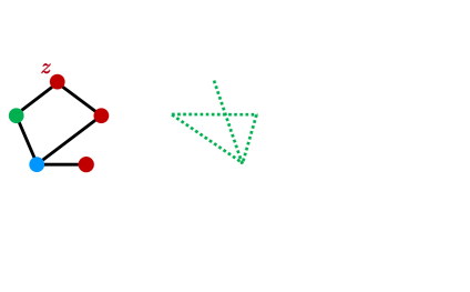
Figure 1: Problem setup. (a) Nodes in $\operatorname{prot}(w)$ colored red; nodes in $\operatorname{pub}(w)$ colored green. (b) $u$ cannot see red edges (solid), red non-edges (dotted) and recommendations ($\pi^{\mathcal{A}}_{\bullet},\bullet\neq u$) to other nodes. $u$ can see green edges (solid), green non-edges (dotted) and recommendation ($\pi^{\mathcal{A}}_{u}$) to itself. (c) Output of ${\overline{\mathcal{A}}}$ should be insensitive to protected pairs.

3 Privacy model for protected pairs

In this section, we first present our privacy model which assesses the privacy loss of protected node-pairs, given the predictions made by an LP algorithm. Then we introduce the sensitivity function, specifically designed for graphs with protected pairs.

3.1 Protected-pair differential privacy

In order to the prevent privacy leakage of the protected connections, we aim to design a privacy preserving LP algorithm ${\overline{\mathcal{A}}}$ based on $\mathcal{A}$, meaning that ${\overline{\mathcal{A}}}$ uses the scores $s_{\mathcal{A}}(u,\cdot)$ to present to each node $u$ a ranking $\pi^{\overline{\mathcal{A}}}_{u}$, while maintaining the privacy of all the protected node pairs in the graph, where one of the two nodes in such a pair is not $u$ itself. We expect that $u$ has strong reasons to link to the top nodes in $\pi^{\overline{\mathcal{A}}}_{u}$, and that the same list will occur again with nearly equal probability, if one changes (adds or deletes) edges between any other node $w$ and the protected nodes of $w$, other than $u$, i.e., $\operatorname{prot}(w)\backslash\{u\}$. We formally define such changes in the graph in the following.

Definition 1 ($u$-neighboring graphs).

Given two graphs $G=(V,E)$ and $G^{\prime}=(V,E^{\prime})$ with the same node set $V$, and a node $u\in V$, we call $G$, $G^{\prime}$ as $u$-neighboring graphs, if there exists some node $w\neq u$ (not necessarily a neighbor), such that

1. protected nodes $\operatorname{prot}(w)$ are the same in $G$ and $G^{\prime}$,

2. public nodes $\operatorname{pub}(w)$ are the same in $G$ and $G^{\prime}$, and

3. $E^{\prime}{\setminus}\{(w,v)\,|\,v{\in}\operatorname{prot}(w)\backslash u\}{=}E{\setminus}\{(w,v)\,|\,v{\in}\operatorname{prot}(w)\backslash u\}$.

The set of all $u$-neighboring graph pairs is denoted as $\mathfrak{N}_{u}$.

In words, the last requirement is that, for the purpose of recommendation to $u$, the information not protected by $w$ is the same in $G$ and $G^{\prime}$. $u$-neighboring graphs may differ only in the protected pairs incident to some other node $w$, except $(w,u)$. Next, we propose our privacy model which characterizes the privacy leakage of protected node-pairs in the context of link prediction.

Definition 2 (Protected-pair differential privacy).

We are given a non-private base LP algorithm $\mathcal{A}$, and a randomized LP routine ${\overline{\mathcal{A}}}$ based on $\mathcal{A}$, which returns a ranking of $K$ nodes. We say that “${\overline{\mathcal{A}}}$ ensures $\epsilon_{p}$-protected-pair differential privacy”, if, for all nodes $u\in V$ and for all ranking $R_{K}$ on the candidate nodes, truncated after position $K$, we have $\Pr(\pi^{\overline{\mathcal{A}}}_{u}=R_{K}\,|\,\mathcal{A},G)\leq e^{\epsilon_{p}}\Pr(\pi^{\overline{\mathcal{A}}}_{u}=R_{K}\,|\,\mathcal{A},G^{\prime})$, whenever $G$ and $G^{\prime}$ are $u$-neighboring graphs.

In words, ${\overline{\mathcal{A}}}$ promises to recommend the same list to $u$, with nearly the same probability, even if we arbitrarily change the protected partners of any node $w$, except for $u$ itself, as that information is already known to $u$. Connections between protected-pair differential privacy and earlier privacy definitions are drawn in Appendix 10.

3.2 Graph sensitivity

Recall that $\mathcal{A}$ recommends $v$ to $u$ based on a score $s_{\mathcal{A}}(u,v)$. A key component of our strategy is to apply a (monotone) transform $f(s_{\mathcal{A}}(u,v))$ to balance it more effectively against samples from a noise generator. To that end, given base LP algorithm $\mathcal{A}$, we define the sensitivity of any function on the scores $f(s_{\mathcal{A}}(u,\cdot)):V\to\mathbb{R}^{+}$, which will be subsequently used to design any protected-pair differentially private LP algorithm.

Definition 3 (Sensitivity of $f\circ s_{\mathcal{A}}$).

The sensitivity $\Delta_{f,\mathcal{A}}$ of a transformation $f$ on the scoring function $s_{\mathcal{A}}$ is defined as

$$\Delta_{f,\mathcal{A}}=\max_{u}\max_{(G,G^{\prime})\in\mathfrak{N}_{u}}\max_{v}\big{|} f(s_{\mathcal{A}}(u,v|G))-f(s_{\mathcal{A}}(u,v|G^{\prime}))\big{|}$$ (1)

Recall $\mathfrak{N}_{u}$ represents all $u$-neighboring graph pairs.

4 Design of privacy protocols for LP

In this section, we first state our problem of designing a privacy preserving LP algorithm ${\overline{\mathcal{A}}}$— based on a non-private LP algorithm $\mathcal{A}$— which aims to provide an optimal trade-off between privacy leakage of the protected node pairs and LP accuracy. Next, we develop DpLp, our proposed algorithm which solves this problem,

4.1 Problem statement

Privacy can always be trivially protected by ignoring private data and sampling each node uniformly, but such an LP ‘algorithm’ has no predictive value. Hence, it is important to design a privacy preserving LP algorithm which can also provide a reasonable LP accuracy. To this end, given a base LP algorithm $\mathcal{A}$, our goal is to design a protected-pair differentially private algorithm ${\overline{\mathcal{A}}}$ based on $\mathcal{A}$, which maximizes the link prediction accuracy. ${\overline{\mathcal{A}}}$ uses random noise, and induces a distribution $\pi^{\overline{\mathcal{A}}}_{u}$ over rankings presented to $u$. Specifically, our goal is solve the following optimization problem:

$$\underset{{\overline{\mathcal{A}}}}{\text{maximize}}\ {\sum_{u\in V}\mathbb{E}_{R_{K}\sim\Pr(\pi^{\overline{\mathcal{A}}}_{u}|\mathcal{A},G)}\text{AUC}(R_{K})}$$ (2)

$$\text{s.t.}\quad{\overline{\mathcal{A}}}\quad\text{is $K\epsilon_{p}$ protected-pair differentially private}.$$

Here, AUC($R_{K}$) measures the area under the ROC curve given by $R_{K}$— the ranked list of recommended nodes truncated at $K$. Hence, the above optimization problem maximizes the expected AUC over the rankings generated by the randomized protocol ${\overline{\mathcal{A}}}$, based on the scores produced by $\mathcal{A}$. The constraint indicates that predicting a single link using ${\overline{\mathcal{A}}}$ requires to satisfy $\epsilon_{p}$-protected-pair differential privacy.

4.2 DpLp: A protected-pair differentially private LP algorithm

A key question is whether well-known generic privacy protocols like Laplace or exponential noising are adequate solvers of the optimization problem in Eq. (2), or might a solution tailored to protected-pair differential privacy in LP do better. We answer in the affirmative by presenting DpLp, a novel DP link predictor, with five salient components.

1. Monotone transformation of the original scores from $\mathcal{A}$.

2. Design of a ranking distribution $\pi^{\overline{\mathcal{A}}}_{u}$, which suitably introduces noise to the original scores to make a sampled ranking insensitive to protected node pairs.

3. Re-parameterization of the ranking distribution to facilitate effective training.

4. Design of a tractable ranking objective that approximates AUC in Eq. (2).

5. Sampling current non-neighbors for recommendation.

Monotone transformation of base scores

We equip ${\overline{\mathcal{A}}}$ with a trainable monotone transformation $f:\mathbb{R}^{+}\to\mathbb{R}^{+}$, which is applied to base scores $s_{\mathcal{A}}(u,\cdot)$. Transform $f$ helps us more effectively balance signal from $\mathcal{A}$ with the privacy-assuring noise distribution we use. We view this transformation from two perspectives.

First, $f(s_{\mathcal{A}}(u,\cdot))$ can be seen as a new scoring function which aims to boost the ranking utility of the original scores $s_{\mathcal{A}}(u,\cdot)$, under a given privacy constraint. In the absence of privacy constraints, we can reasonably demand that the ranking quality of $f\circ s_{\mathcal{A}}$ be at least as good as $s_{\mathcal{A}}$. In other words, we expect that the transformed and the original scores provide the same ranking utility, i.e., the same list of recommended nodes, in the absence of privacy constraints. A monotone $f$ ensures such a property.

Second, as we shall see, $f$ can also be seen as a probability distribution transformer. Given a sufficiently expressive neural representation of $f$ (as designed in Section 4.3), any arbitrary distribution on the original scores can be fitted with a tractable known distribution on the transformed scores. This helps us build a high-capacity but tractable ranking distribution $\Pr(\pi^{\overline{\mathcal{A}}}_{u}\,|\,\mathcal{A},G)$, as described below.

Design of a ranking distribution

Having transformed the scores $s_{\mathcal{A}}(u,.)$ into $f(s_{\mathcal{A}}(u,v))$, we draw nodes $v$ using an iterative exponential mechanism on the transformed scores $f(s_{\mathcal{A}}(u,v))$. Specifically, we draw the first node $v$ with probability proportional to $\exp\left({\epsilon_{p}f(s_{\mathcal{A}}(u,v))}/2{\Delta_{f,\mathcal{A}}}\right)$, then repeat for collecting $K$ nodes in all. Thus, our ranking distribution in Eq. (2) is:

$$\Pr(\pi^{\overline{\mathcal{A}}}_{u} =R_{K}|\mathcal{A},G)=\displaystyle\prod_{j=1}^{K}\dfrac{\exp\left(\dfrac{\epsilon_{p}f(s_{\mathcal{A}}(u,R_{K}(j)))}{2\Delta_{f,\mathcal{A}}}\right)}{{\sum_{w\not\in R_{K}(1,..,j-1)}}\exp\left(\dfrac{\epsilon_{p}f(s_{\mathcal{A}}(u,w))}{2\Delta_{f,\mathcal{A}}}\right)},$$ (3)

In the absence of privacy concerns ($\epsilon_{p}\to\infty$), the candidate node with the highest score $f(s_{\mathcal{A}}(u,.))$ gets selected in each step, and the algorithm reduces to the original non-private LP algorithm $\mathcal{A}$, thanks to the monotonicity of $f$. On the other hand, if $\epsilon_{p}\to 0$, then every node has an equal chance of getting selected, which preserves privacy but has low predictive utility.

Indeed, our ranking distribution in Eq. (3) follows an exponential mechanism on the new scores $f(s_{\mathcal{A}}(u,\cdot))$. However, in principle, such a mechanism can capture any arbitrary ranking distribution $\Pr(\pi^{\overline{\mathcal{A}}}_{u}|\mathcal{A},G)$, given sufficient training and expressiveness of $f$.

Finally, we note that $f$ can be designed to limit $\Delta_{f,\mathcal{A}}$. E.g., if we can ensure that $f(\cdot)$ is positive and bounded by $B$, then we can have $\Delta_{f,\mathcal{A}}\leq B$; if we can ensure that the derivative $f^{\prime}(\cdot)$ is bounded by $B^{\prime}$, then, by the Lipschitz property, $\Delta_{f,\mathcal{A}}\leq B^{\prime}\Delta_{\mathcal{A}}$.

Re-parameterization of the ranking distribution

In practice, the above-described procedure for sampling a top-$K$ ranking results in high estimation variance during training [55, 34, 41, 44]. To overcome this problem, we make a slight modification to the softmax method. We first add i.i.d Gumbel noise $\eta_{u,v}\sim\textsc{Gum}(2\Delta_{f,\mathcal{A}}/\epsilon_{p})$ to each score $f(s_{\mathcal{A}}(u,v))$ and then take top $K$ nodes with highest noisy score [10, Lemma 4.2]. Such a distribution allows an easy re-parameterization trick — $\textsc{Gum}(2\Delta_{f,\mathcal{A}}/\epsilon_{p})=(2\Delta_{f,\mathcal{A}}/\epsilon_{p})\cdot\textsc{Gum}(1)$ — which reduces the parameter variance. With such a re-parameterization of the softmax ranking distribution in Eq. (3), we get the following alternative representation of our objective in Eq. (2):

$${{\sum_{u\in V}}\underset{\{\eta_{u,\bullet}\}}{\mathbb{E}}\underset{\sim\textsc{Gum}(1)}{}\text{AUC}\left(R_{K}\bigg{(}\bigg{\{}f(s_{\mathcal{A}}(u,\bullet)+\tfrac{2\Delta_{f,\mathcal{A}}\eta_{u,\bullet}}{\epsilon_{p}}\bigg{\}}\bigg{)}\right)},$$

where $R_{K}(.)$ gives a top-$K$ ranking based on the noisy transformed scores $\{f(s_{\mathcal{A}}(u,\bullet)+{2\Delta_{f,\mathcal{A}}\eta_{u,\bullet}}/{\epsilon_{p}}\}$ over the candidate nodes for recommendation to $u$.

Designing a tractable ranking objective

Despite the aforementioned re-parameterization trick, standard optimization tools face several challenges to maximize the above objective. First, optimizing AUC is an NP-hard problem. Second, truncating the list up to $K$ nodes often pushes many neighbors out of the list at the initial stages of learning, which can lead to poor training [31]. To overcome these limitations, we replace AUC [14] with a surrogate pairwise hinge loss $\ell(\cdot)$ and consider a non-truncated list $R_{|V|-1}$ of all possible candidate nodes during training [14, 22]. Hence our optimization problem becomes:

$$\underset{f}{\text{min}}\ {\sum_{u\in V}}\ {\mathbb{E}}_{\{\eta_{u,\bullet}\}\sim\textsc{Gum}(1)}{}\ell\left(\left\{f(s_{\mathcal{A}}(u,\bullet)),\eta_{u\bullet}\right\};G\right)$$ (4)

where $\ell\left(\left\{f(s_{\mathcal{A}}(u,\bullet)),\eta_{u\bullet}\right\};G\right)$ is given by a pairwise ranking loss surrogate over the noisy transformed scores:

$$\sum_{\begin{subarray}{c}g\in\operatorname{nbr}(u)\cap\operatorname{pub}(u)\\ b\in\operatorname{\overline{\operatorname{nbr}}}(u)\cap\operatorname{pub}(u)\end{subarray}}\text{ReLU}\bigg{[}\varrho+f(s_{\mathcal{A}}(u,b))+\dfrac{2\Delta_{f,\mathcal{A}}\eta_{ub}}{\epsilon_{p}}-f(s_{\mathcal{A}}(u,g))-\dfrac{2\Delta_{f,\mathcal{A}}\eta_{ug}}{\epsilon_{p}}\bigg{]}.$$ (5)

The above loss function encourages that the (noisy) transformed score of a neighbor $g$ exceeds the corresponding score of a non-neighbor $b$ by at least (a tunable) margin $\varrho$. In absence of privacy concern, i.e., $\epsilon_{p}\to\infty$, it is simply $\text{ReLU}\left[\varrho+f(s_{\mathcal{A}}(u,b))-f(s_{\mathcal{A}}(u,g))\right]$, which would provide the same ranking as $\mathcal{A}$, due to the monotonicity of $f$.

We would like to point out that the objective in Eq 5 uses only non-protected pairs $\{(u,v)|v\in\operatorname{pub}(u)\}$ to train $f$. This ensures no privacy is leaked during training.

Algorithm 1 DpLp: Learns ${\overline{\mathcal{A}}}$ based on a non-private LP algorithm $\mathcal{A}$ and then uses it to recommend $K$ nodes to $u$.

1:  Input $G=(V,E)$; protected and non-protected node-sets $\operatorname{prot}(\cdot),\operatorname{pub}(\cdot)$; scores $s_{\mathcal{A}}(.,.)$ given by $\mathcal{A}$; privacy leakage $\epsilon_{p}$, margin $\varrho$.

2:  Output $R_{K}:$ List of top-$K$ recommended nodes to node $u$

3:  Initialize $R_{K}(1\ldots K)\leftarrow\emptyset$

4:  $f\leftarrow$ Train$\left(G,\{s_{\mathcal{A}}(w,v)\,|\,v\in\operatorname{pub}(w),u\in V\},\epsilon_{p},\varrho\right)$

5:  $\text{candidates}\leftarrow\operatorname{\overline{\operatorname{nbr}}}(u)$

6:  for $j$ in $1\ldots K$ do

7:     $w\sim\textsc{SoftMax}\left(\{\epsilon_{p}f(s_{\mathcal{A}}(u,v)/2\Delta_{f,\mathcal{A}}\,|\,v\in\text{candidates}\}\right)$

8:     $\text{candidates}\leftarrow\text{candidates}\backslash\{w\}$

9:     $R_{K}(j)\leftarrow w$

10:  Return $R_{K}$

Sampling nodes for recommendation. Once we train $f$ by solving the optimization problem in Eq. (4), we draw top-$K$ candidate nodes using the trained $f$. Specifically, we first sample a non-neighbor $v$ with probability proportional to $\exp\left(\epsilon_{p}f(s_{\mathcal{A}}(u,v))/2\Delta_{f,\mathcal{A}}\right)$ and then repeat the same process on the remaining non-neighbors $\operatorname{\overline{\operatorname{nbr}}}(u)\backslash\{v\}$ and continue $K$ times.

Overall algorithm. We summarize the overall algorithm in Algorithm 1, where the $\textsc{Train}(\bullet)$ routine solves the optimization problem in Eq. (4). Since there is no privacy leakage during training, the entire process — from training to test — ensures $K\epsilon_{p}$ protected-pair differential privacy, which is formalized in the following proposition and proven in Appendix 11.

Proposition 4.

Algorithm 1 implements $K\epsilon_{p}$-protected-pair differentially private LP.

Incompatibility with node and edge DP

Note that, our proposal is incompatible with node or edge privacy (where each node or edge is protected). In those cases, objective in Eq. (5) cannot access any data in the training graph. However, our proposal is useful in many applications like online social networks, in which, a user usually protects a fraction of his sensitive connections, while leaving others public.

4.3 Structure of the monotonic transformation

We approximate the required nonlinear function $f$ with $f_{\bm{\theta}}$, implemented as a monotonic neural network with parameters $\bm{\theta}$. Initial experiments suggested that raising the raw score $s_{\mathcal{A}}(u,v)$ to a power $a>0$ provided a flexible trade-off between privacy and utility over diverse graphs. We provide a basis set $\{a_{i}>0\}$ of fixed powers and obtain a positive linear combination over raw scores $s_{\mathcal{A}}(u,\cdot)$ raised to these powers. More specifically, we compute:

$$\nu_{\bm{\beta}}(s_{\mathcal{A}}(u,v))=\sum_{i=1}^{n_{a}}e^{\tau\beta_{i}}(s_{\mathcal{A}}(u,v))^{a_{i}},$$ (6)

where $(a_{i})_{i\in[n_{a}]}>0$ are fixed a priori. $\bm{\beta}=(\beta_{i})_{i\in[n_{a}]}$ are trainable parameters and $\tau$ is a temperature hyperparameter. This gave more stable gradient updates than letting $a$ float as a variable.

While using $\nu_{\bm{\beta}}(s_{\mathcal{A}}(u,v))$ as $f(s_{\mathcal{A}}(u,v))$ is already an improvement upon raw score $s_{\mathcal{A}}(u,v)$, we propose a further refinement: we feed $\nu_{\bm{\beta}}(s_{\mathcal{A}}(u,v))$ to a Unconstrained Monotone Neural Network (UMNN) [52] to finally obtain $f_{\bm{\theta}}(s_{\mathcal{A}}(u,v))$. UMNN is parameterized using the integral of a positive nonlinear function:

$$f_{\bm{\theta}}(s_{\mathcal{A}}(u,v))=\int_{0}^{\nu_{\bm{\beta}}(s_{\mathcal{A}}(u,v))}g_{\bm{\phi}}(s)ds+b_{0},~{}$$ (7)

where $g_{\bm{\phi}}(.)$ is a positive neural network, parameterized by $\bm{\phi}$. UMNN offers an unconstrained, highly expressive parameterization of monotonic functions, since the monotonicity herein is achieved by only enforcing a positive integrand $g_{\bm{\phi}}(\cdot)$. In theory, with sufficient training and capacity, a ‘universal’ monotone transformation may absorb $\nu_{\beta}(\cdot)$ into its input stage, but, in practice, we found that omitting $\nu_{\beta}(\cdot)$ and passing $s_{\mathcal{A}}(u,v)$ directly to UMNN gave poorer results (Appendix 15). Therefore, we explicitly provide $\nu_{\bm{\beta}}(s_{\mathcal{A}}(u,v))$ as an input to it, instead of the score $s_{\mathcal{A}}(u,v)$ itself. Overall, we have $\bm{\theta}=\{\bm{\beta},\bm{\phi},b_{0}\}$ as the trainable parameters.

5 Privacy-accuracy trade-off of DpLp

It is desirable that a privacy preserving LP algorithm should be able to hide the protected node-pairs as well as give high predictive accuracy. However, in principle, LP accuracy is likely to deteriorate with higher privacy constraint (lower $\epsilon_{p}$). For example, a uniform ranking distribution, i.e., $\epsilon_{p}{\to}0$ provides extreme privacy. However, it would lead to a poor prediction. On the other hand, in absence of privacy, i.e., when $\epsilon_{p}\to\infty$, the algorithm enjoys an unrestricted use of the protected pairs, which is likely to boost its accuracy. In this section, we analyze this trade-off from two perspectives.

1. Relative trade-off analysis. Here, we assess the relative loss of prediction quality of ${\overline{\mathcal{A}}}$ with respect to the observed scores of the the base LP algorithm $\mathcal{A}$.

2. Absolute trade-off analysis. Here, we assess the loss of absolute prediction quality of ${\overline{\mathcal{A}}}$ with respect to the true utility provided by a latent graph generative process.

5.1 Relative trade-off analysis

Like other privacy preserving algorithms, DpLp also introduces some randomness to the base LP scores, and therefore, any DpLp algorithm ${\overline{\mathcal{A}}}$ may reduce the predictive quality of $\mathcal{A}$. To formally investigate the loss, we quantify the loss in scores suffered by ${\overline{\mathcal{A}}}$, compared to $\mathcal{A}$:

$$\gamma_{u}(\mathcal{A},\epsilon_{p})=\mathbb{E}_{{\overline{\mathcal{A}}}}\bigg{[}\sum_{i\in[K]}s_{\mathcal{A}}(u,u^{\mathcal{A}}_{i}|G)-\sum_{i\in[K]}s_{\mathcal{A}}(u,u^{{\overline{\mathcal{A}}}}_{i}|G)\bigg{]}.$$

Recall that $u^{\mathcal{A}}_{i}=\pi^{\mathcal{A}}_{u}(i)$ and $u^{\overline{\mathcal{A}}}_{i}=\pi^{\overline{\mathcal{A}}}_{u}(i)$. We do not take absolute difference because the first term cannot be smaller than the second. The expectation is over randomness introduced by the algorithm ${\overline{\mathcal{A}}}$. The following theorem bounds $\gamma_{u}(\mathcal{A},\epsilon_{p})$ in two extreme cases (Proven in Appendix 12).

Proposition 5.

If $\epsilon_{p}$ is the privacy parameter and $\kappa_{u,\mathcal{A}}:=\max_{i\in[|V|-1]}\{s_{\mathcal{A}}(u,u^{\mathcal{A}}_{i})-s_{\mathcal{A}}(u,u^{\mathcal{A}}_{i+1})\}$, then we have:

$$\lim_{\epsilon_{p}\to\infty}\gamma_{u}(\mathcal{A},\epsilon_{p})=0\text{ and, }\lim_{\epsilon_{p}\to 0}\gamma_{u}(\mathcal{A},\epsilon_{p})\leq K\kappa_{u,\mathcal{A}}.$$

Here, $\kappa_{u,\mathcal{A}}$ gives maximum difference between the scores of two consecutive nodes in the ranking provided by $\mathcal{A}$ to $u$.

5.2 Absolute trade-off analysis

Usually, $\mathcal{A}$ provides only imperfect predictions. Hence, the above trade-off analysis which probes into the relative cost of privacy with respect to $\mathcal{A}$, may not always reflect the real effect of privacy on the predictive quality. To fill this gap, we need to analyze the absolute prediction quality — utility in terms of the true latent generative process — which is harder to analyze. Even for a non-private LP algorithms $\mathcal{A}$, absolute quality is rarely analyzed, except for Sarkar et al. [43], which we discuss below.

Latent space network model

We consider the latent space model proposed by Sarkar et al. [43], which showed why some popular LP methods succeed. In their model, the nodes lie within a $D$-dimensional hypersphere having unit volume. Each node $u$ has a co-ordinate $\bm{x}_{u}$ within the sphere, drawn uniformly at random. Given a parameter $r>0$, the latent generative rule is that nodes $u$ and $v$ get connected if the distance $d_{uv}=||\bm{x}_{u}-\bm{x}_{v}||_{2}<r$.

Relating ranking loss to absolute prediction error

If an oracle link predictor could know the underlying generative process, then its ranking $\pi^{*}_{u}$ would have sorted the nodes in the increasing order of distances $d_{u\bullet}$. An imperfect non-private LP algorithm $\mathcal{A}$ does not have access to these distances and therefore, it would suffer from some prediction error. ${\overline{\mathcal{A}}}$, based on $\mathcal{A}$, will incur an additional prediction error due to its privacy preserving randomization. We quantify this absolute loss by extending our loss function in Eq. (4):

$$\operatorname{\ell}(\pi^{\overline{\mathcal{A}}}_{u};\pi^{*}_{u}):=\textstyle{\sum_{{i<j\leq K}}[d_{uu^{\overline{\mathcal{A}}}_{i}}-d_{uu^{\overline{\mathcal{A}}}_{j}}]_{+}.}$$ (8)

Here, recall that $u^{\overline{\mathcal{A}}}_{i}=\pi^{\overline{\mathcal{A}}}_{u}(i)$. Analyzing the above loss for any general base LP method, especially deep embedding methods like GCN, is extremely challenging. Here we consider simple triad based models e.g., Adamic Adar (AA), Jaccard coefficients (JC) and common neighbors (CN). For such base LP methods, we bound this loss in the following theorem (proven in Appendix 12).

Theorem 6.

Given $\epsilon=\sqrt{\frac{2\log(2/\delta)}{|V|}}+\frac{7\log(2/\delta)}{3(|V|-1)}$. For $\mathcal{A}\in\{\text{AA},\text{CN},\text{JC}\}$, with probability $1-4K^{2}\delta$:

$$\mathbb{E}_{{{\overline{\mathcal{A}}}}}\left[\operatorname{\ell}(\pi^{\overline{\mathcal{A}}}_{u};\pi^{*}_{u})\right]=O\left(\big{[}2K\epsilon+{\gamma_{u}(\mathcal{A},\epsilon_{p})}/{|V|}\big{]}^{\frac{1}{KD}}\right),$$ (9)

where $D$ is the dimension of the underlying hypersphere for the latent space random graph model.

The $2K\epsilon$ term captures the predictive loss due to imperfect LP algorithm $\mathcal{A}$ and $\gamma_{u}(\mathcal{A},\epsilon_{p})/|V|$ characterizes the excess loss from privacy constraints. Note that $\epsilon$ here is unrelated to privacy level $\epsilon_{p}$; it characterizes the upper bounds of the expected losses due to $\mathcal{A}$, and it depends on $\delta$ that quantifies the underlying confidence interval. The expectation is taken over random choices made by differentially private, and not randomness in the process generating the data.

6 Experiments

	AA						CN
	$\mathcal{A}$	DpLp	DpLp-Lin	Staircase	Lapl.	Exp.	$\mathcal{A}$	DpLp	DpLp-Lin	Staircase	Lapl.	Exp.
Facebook	0.842	0.788	0.211	0.163	0.168	0.170	0.827	0.768	0.544	0.169	0.181	0.177
USAir	0.899	0.825	0.498	0.434	0.461	0.423	0.873	0.819	0.670	0.432	0.482	0.435
Twitter	0.726	0.674	0.517	0.504	0.515	0.488	0.718	0.667	0.630	0.505	0.523	0.493
Yeast	0.778	0.696	0.179	0.154	0.154	0.149	0.764	0.667	0.359	0.146	0.160	0.151
PB	0.627	0.558	0.287	0.254	0.263	0.255	0.593	0.537	0.389	0.277	0.272	0.257
	GCN						Node2Vec
	$\mathcal{A}$	DpLp	DpLp-Lin	Staircase	Lapl.	Exp.	$\mathcal{A}$	DpLp	DpLp-Lin	Staircase	Lapl.	Exp.
Facebook	0.463	0.151	0.154	0.159	0.145	0.150	0.681	0.668	0.202	0.157	0.152	0.155
USAir	0.483	0.446	0.391	0.389	0.399	0.420	0.752	0.681	0.424	0.403	0.422	0.447
Twitter	0.504	0.496	0.498	0.516	0.509	0.505	0.608	0.555	0.511	0.485	0.512	0.505
Yeast	0.369	0.163	0.131	0.116	0.125	0.112	0.836	0.803	0.180	0.151	0.159	0.145
PB	0.503	0.287	0.293	0.262	0.286	0.261	0.525	0.473	0.304	0.266	0.282	0.255

Table 1: Performance (AUC) for base non-private LP algorithm $\mathcal{A}$ and five different DP protocols ${\overline{\mathcal{A}}}$, viz., DpLp, DpLp-Lin, Staircase [15], Laplace [33] and Exponential [33] on 20% held-out set. Four base LP algorithms $\mathcal{A}$ i.e., AA, CN, GCN, Node2Vec, across all five datasets. We set the fraction of protected pairs $\sigma_{\text{prot}}=0.3$, the privacy leakage $\epsilon_{p}=0.1$ and the number of recommended nodes $K=30$. Baseline LP algorithms AA and CN are triad-based. Baselines GCN and Node2Vec are based on node embeddings. Bold numbers correspond to the best performing ${\overline{\mathcal{A}}}$, for the given base algorithm $\mathcal{A}$. DpLp outperforms all other candidates of ${\overline{\mathcal{A}}}$ for all LP algorithms $\mathcal{A}$, except for GCN, in which, Staircase and DpLp-Lin also outperform DpLp in several datasets.

We report on experiments with five real world datasets to show that DpLp can trade off privacy and the predictive accuracy more effectively than three standard DP protocols [15, 33, 36].

6.1 Experimental setup

Datasets

We use five networks: Facebook [28], USAir [6], Twitter [28], Yeast [50], PB [2]. Appendix 14 gives further details about them.

Evaluation protocol and metrics

For each of these datasets, we first mark a portion ($\sigma_{\text{prot}}$) of all connections to be protected. Following previous work [3, 9], we sort nodes by decreasing number of triangles in which they occur, and allow the top 80% to be query nodes. Next, for each query node $q$ in the disclosed graph, the set of nodes $V\backslash\{q\}$ is partitioned into neighbors $\operatorname{nbr}(q)$ and non-neighbors ${\operatorname{\overline{\operatorname{nbr}}}(q)}$. Finally, we sample 80% of $|\operatorname{nbr}(q)|$ neighbors and 80% of ${\operatorname{\overline{\operatorname{nbr}}}(q)}$ non-neighbors and present the resulting graph $G_{\text{sampled}}$ to $\mathcal{A}$—the non-private base LP, and subsequently to ${\overline{\mathcal{A}}}$—the protected-pair differentially private LP which is built on $\mathcal{A}$. For each query node $q$, we ask ${\overline{\mathcal{A}}}$ to provide a top-$K$ list of potential neighbors from the held-out graph, consisting of both public and private connections. We report the predictive performance of ${\overline{\mathcal{A}}}$ in terms of average AUC of the ranked list of nodes across all the queries $Q$. The exact choices of $\sigma_{\text{prot}}$ and $K$ vary across different experiments.

Candidates for base LP algorithms $\mathcal{A}$

We consider two classes of base LP algorithms $\mathcal{A}$: (i) algorithms based on the triad-completion principle [30] viz., Adamic Adar (AA) and Common Neighbors (CN); and, (ii) algorithms based on fitting node embeddings, viz., GCN [26] and Node2Vec [18]. In Appendix 14, we provide the details about implementation of these algorithms. Moreover, in Appendix 15, we also present results on a wide variety of LP protocols.

DpLp and baselines (${\overline{\mathcal{A}}}$)

We compare DpLp against three state-of-the-art perturbation methods i.e., Staircase [15], Laplace [33] and Exponential [33, 36], which maintain differential privacy off-the-shelf. Moreover, as an ablation, apart from using $\nu_{\bm{\beta}}(.)$ — the linear aggregator of different powers of the score — as a signal in $f_{\bm{\theta}}(.)$ (Eqs. 6 and  7), we also use it as an independent baseline i.e., $f_{\bm{\theta}}(s)=\nu_{\bm{\beta}}(s)$ with $\bm{\theta}=\{\bm{\beta}\}$. We refer such a linear “monotone transformation” as DpLp-Lin. In Appendix 15, as another ablation, we consider another variant of DpLp, which directly uses the scores $s_{\mathcal{A}}(u,v)$ as inputs to UMNN (Eq. 7), instead of its linear powers $\nu_{\bm{\beta}}(s_{\mathcal{A}}(u,v))$. Appendix 14 provides the implementation details about DpLp and baselines.

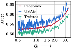
Figure 2: AUC vs. $a$. $f(s_{\mathcal{A}}(u,v))$ $=(s_{\mathcal{A}}(u,v))^{a}$ and the base LP algorithm is common neighbors i.e., $\mathcal{A}=\text{CN}$.

6.2 Results

We first present some empirical evidence which motivates our formulation of $f$, specifically, the choice of the component $\nu_{\bm{\beta}}(s_{\mathcal{A}}(\cdot,\cdot))$. We draw nodes using exponential mechanism with different powers of the scores. To recommend neighbors to node $u$, we draw nodes from the distribution in Eq. (3), with $f(s_{\mathcal{A}}(u,\cdot))=(s_{\mathcal{A}}(u,\cdot))^{a}$ for different values of $a$. Figure 2 illustrates the results for three datasets with the fraction of protected connections $\sigma_{\text{prot}}=0.3$, the privacy leakage $\epsilon_{p}=0.1$ and $\mathcal{A}=\text{CN}$. It shows that AUC improves as $a$ increases. This is because, as $a$ increases, the underlying sampling distribution induced by the exponential mechanism with new score $f(s_{\text{CN}})=s_{\text{CN}}^{a}$ becomes more and more skewed towards the ranking induced by the base scores $s_{\mathcal{A}}$, while maintaining privacy level $\epsilon_{p}$. It turns out that use of UMNN in Eq. (7) further significantly boosts predictive performance of DpLp.

We compare DpLp against three state-of-the-art DP protocols (Staircase, Laplace and exponential), at a given privacy leakage $\epsilon_{p}=0.1$ and a given fraction of protected edges $\sigma_{\text{prot}}=0.3$, for top-$K$ (=30) predictions. Table 1 summarizes the results, which shows that DpLp outperforms competing DP protocols, including its linear variant DpLp-Lin, for $\mathcal{A}=\text{AA},\text{CN}$ and Node2Vec. There is no consistent winner in case of GCN, which is probably because GCN turns out be not-so-good link predictor in our datasets.

Next, we study how AUC of all algorithms vary as the fraction of protected pairs $\sigma_{\text{prot}}$ and the permissible privacy leakage level $\epsilon_{p}$ change. Figure 3 summarizes the results for Yeast dataset, which shows that our method outperforms the baselines for almost all values of $\sigma_{\text{prot}}$ and $\epsilon_{p}$.

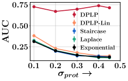
(a)

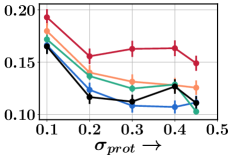
(b)

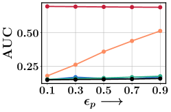
(b) $\mathcal{A}=\text{AA}$

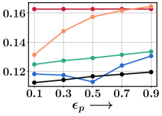
(c) $\mathcal{A}=\text{GCN}$

Figure 3: Variation of AUC with $\sigma_{\text{prot}}$ (top row) and with $\epsilon_{p}$ (bottom row) for all candidates of ${\overline{\mathcal{A}}}$ with $\mathcal{A}=\text{AA}$ and $\mathcal{A}=\text{GCN}$ for Yeast dataset. For top row, we set $\epsilon_{p}=0.1$ and for bottom row, we set $\sigma_{\text{prot}}=0.3$.

The AUC achieved by DpLp is strikingly stable across a wide variation these parameters. This apparently contradicts the natural notion of utility-privacy tradeoff: increasing utility should decrease privacy. The apparent conundrum is resolved when we recognize that $f_{\bm{\theta}}$ adapts to each level of permissible privacy leakage, providing different optimal $f$s. In contrast, Laplace and Exponential mechanisms use the same score values for different $\epsilon_{p}$. Therefore, as $\epsilon_{p}$ decreases, the underlying perturbation mechanism moves quickly toward the uniform distribution. While both Staircase and DpLp-Lin aim to find optimal noise distributions, Staircase is not optimized under ranking utility and DpLp-Lin is constrained by its limited expressiveness. Therefore, they fare poorly.

7 Conclusion

We proposed protected-pair differential privacy, a practically motivated variant of differential privacy for social networks. Then we presented DpLp, a noising protocol designed around a base non-private LP algorithm. DpLp maximizes ranking accuracy, while maintaining a specified privacy level of protected pairs. It transforms the base score using a trainable monotone neural network and then introduces noise into these transformed scores to perturb the ranking distribution. DpLp is trained using a pairwise ranking loss function. We also analyzed the loss of ranking quality in a latent distance graph generative framework. Extensive experiments show that DpLp trades off ranking accuracy and privacy better than several baselines. Our work opens up several interesting directions for future work. E.g., one may investigate collusion between queries and graph steganography attacks [4]. One may also analyze utility-privacy trade-off in other graph models e.g., Barabási-Albert graphs [5], Kronecker graphs [29], etc.

8 Broader Impact

Privacy concerns have increased with the proliferation of social media. Today, law enforcement authorities routinely demand social media handles of visa applicants [37]. Insurance providers can use social media content to set premium levels [38]. One may avoid such situations, by making individual features e.g., demographic information, age, etc. private. However, homophily and other network effects may still leak user attributes, even if they are made explicitly private. Someone having skydiver or smoker friends may end up paying large insurance premiums, even if they do not subject themselves to those risks. A potential remedy is for users to mark some part of their connections as private as well [51]. In our work, we argue that it is possible to protect privacy of such protected connections, for a specific graph based application, i.e., link prediction, while not sacrificing the quality of prediction. More broadly, our work suggests that, a suitably designed differentially private algorithm can still meet the user expectation in social network applications, without leaking user information.

Differentially Private Link Prediction
With Protected Connections
(Appendix)

Roadmap to different parts of appendix

• Appendix 9 contains formal definitions of node differential privacy, edge differential privacy and protected-pair differential privacy in a broader context.

• Appendix 10 connects protected-node-pair differential privacy with other variants of differential privacy.

• Appendix 11 contains proof of Proposition 4, i.e., the privacy guarantee of Algorithm 1.

• Appendix 12 shows the proofs of the technical results presented in Section 5. More specifically, here we bound the relative (Proposition 5) and absolute (Theorem 6) trade-off between privacy and LP accuracy.

• Appendix 13 provides auxiliary theoretical results, required to prove the results of Appendix 12.

• Appendix 14 provides additional experimental details.

• Appendix 15 provides additional experiments.

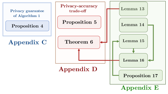
Figure 4: Inter-dependence between the theoretical results presented in Appendix. Appendix C proves privacy guarantee of Algorithm 1. Appendix D contains proofs on privacy-utility trade-off. Appendix E contains auxiliary results. $$A$$$\to$$$B$$ means that $A$ is used to prove $B$.

9 Formal definition of node differential privacy, edge differential privacy,
protected-pair differential privacy

Any algorithm $\mathcal{M}$ on a graph is $\epsilon_{p}$ differentially private [33], if, we have ${\Pr(\mathcal{M}(G)\in\mathcal{O})}\leq\exp(\epsilon_{p}|G\oplus G^{\prime}|){\Pr(\mathcal{M}(G^{\prime})\in\mathcal{O})}$ where $G^{\prime}$ (called as a neighbor graph of $G$) is obtained by perturbing $G$. $|G\oplus G^{\prime}|$ measures the extent of perturbation between $G$ and $G^{\prime}$. In order to apply DP on graphs, we need to quantify the granularity of such a perturbation, or in other words, define the neighborhood criteria of two graphs $G$ and $G^{\prime}$. Existing work predominantly considers two types of DP formulations on graphs: (i) edge differential privacy (edge DP), where $G$ and $G^{\prime}$ differ by one edge [39, 19] and, (ii) node differential privacy (node DP), where $G$ and $G^{\prime}$ differ by a node and all its incident edges [7, 23, 47].

Definition 7 (Node DP).

Two graphs $\mathcal{G}=(V,E)$ and $\mathcal{G}^{\prime}=(V,E^{\prime})$ with the same node set $V$ are neighboring if $E\neq E^{\prime}$ and there exists a node $u$ such that $E\backslash\{(u,v)|v\in V\backslash\{u\}\}=E^{\prime}\backslash\{(u,v)|v\in V\backslash\{u\}\}$. Then an algorithm $\mathcal{M}$ is $\epsilon_{p}$ node DP if, for any two neighboring graphs $G,G^{\prime}$, we have:

$$\Pr(\mathcal{M}(G)\in\mathcal{O})\leq e^{\epsilon_{p}}\Pr(\mathcal{M}(G^{\prime})\in\mathcal{O})$$ (10)

Definition 8 (Edge DP).

Two graphs $\mathcal{G}=(V,E)$ and $\mathcal{G}^{\prime}=(V,E^{\prime})$ with the same node set $V$ are neighboring if $E\neq E^{\prime}$ and there exists a node pair $(u,v)$, such that $E\backslash\{(u,v)\}=E^{\prime}\backslash\{(u,v)\}$. Then an algorithm $\mathcal{M}$ is $\epsilon_{p}$ edge DP if, for any two neighboring graphs $G,G^{\prime}$ we have:

$$\Pr(\mathcal{M}(G)\in\mathcal{O})\leq e^{\epsilon_{p}}\Pr(\mathcal{M}(G^{\prime})\in\mathcal{O})$$ (11)

Definition 9 (Protected-node-pair DP).

We are given a randomized algorithm $\mathcal{M}$ which operates on each node $u\in V$. We say that “$\mathcal{M}$ ensures $\epsilon_{p}$-protected-pair differential privacy”, if, for all nodes $u\in V$ we have

$$\Pr(\mathcal{M}(G,u)\in\mathcal{O})\leq e^{\epsilon_{p}}\Pr(\mathcal{M}(G^{\prime},u)\in\mathcal{O}),$$ (12)

whenever $G$ and $G^{\prime}$ are $u$-neighboring graphs (See Definition 1).

Neighboring graphs $G,G^{\prime}$ have $|G\oplus G^{\prime}|=1$ for node DP, edge DP and Protected-node-pair DP.

10 Connection of protected-node-pair differential privacy with other variants of differential privacy

In the following, we relate our proposed privacy model on graphs with three variants of differential privacy e.g., group privacy, Pufferfish privacy and Blowfish privacy.

Connection with group privacy

Our privacy proposal can be cast as an instance of group privacy [11, 46], where the goal is to conceal the information of protected groups.

Definition 10 (Group privacy).

Given a database $\mathcal{D}$ and a collection of subsets containing sensitive information: $\textsc{Priv}=\{P_{1},P_{2},\cdots,P_{k}\}$ with $P_{i}\subset\mathcal{D}$. An algorithm $\mathcal{M}$ is $\epsilon_{p}$ group differentially private w.r.t Priv if for all $P_{i}$ in Priv for all pairs of $\mathcal{D}$ and $\mathcal{D}^{\prime}$ which differ in the entries in $P_{i}$ i.e., $\mathcal{D}\backslash P_{i}=\mathcal{D}^{\prime}\backslash P_{i}$, we have:

$$\Pr(\mathcal{M}(\mathcal{D})\in\mathcal{O})\leq e^{\epsilon_{p}}\Pr(\mathcal{M}(\mathcal{D}^{\prime})\in\mathcal{O})\ \forall\ \mathcal{O}\in\text{Range}(\mathcal{M})$$ (13)

Note that in the context of our current problem, if we have $\mathcal{D}=G,\mathcal{D}^{\prime}=G^{\prime}$, with $G$ and $G^{\prime}$ being $u$-neighboring graphs; $P_{w}=\{(v,w)|v\in\operatorname{prot}(w)\backslash u\}$; and, $\mathcal{M}$ to be a randomized LP algorithm which operates on $u$, then, Definition 9 shows that our privacy model closely related group privacy. However, note that since the sensitive information differs across different nodes, the set Priv also varies across different nodes.

Connection with Pufferfish privacy

Our privacy proposal is also connected with Pufferfish privacy [25, 46]. In Pufferfish privacy, we define three parameters: $\mathcal{S}$ which contains the sensitive information; $\mathcal{Q}\subseteq\mathcal{S}\times\mathcal{S}$ which contains the set of pairs, that we want to be indistinguishable; and, $\Gamma$ a set data distributions. In terms of these parameters, we define Pufferfish privacy as follows.

Definition 11 (Pufferfish privacy [25, 46]).

Given the tuple $(\mathcal{S},\mathcal{Q},\Gamma)$, an algorithm $\mathcal{M}$ is said to be $\epsilon_{p}$ Pufferfish private if for all $\zeta\in\Gamma$ with $\mathcal{D}$ drawn from distribution $\zeta$, for all $(a_{i},a_{j})\in\mathcal{Q}$, we have:

$$\log\left|\dfrac{\Pr(\mathcal{M}(\mathcal{D})\in\mathcal{O}\,|\,a_{i},\zeta)}{\Pr(\mathcal{M}(\mathcal{D})\in\mathcal{O}\,|\,a_{j},\zeta)}\right|<\epsilon_{p}\ \forall\ \mathcal{O}\ \in\text{Range}(\mathcal{M})\ \text{ and }\Pr(a_{i}|\zeta)\neq 0,\ \Pr(a_{j}|\zeta)\neq 0.$$ (14)

In the context of social networks, where users have marked private edges, one can naturally model $\mathcal{S}$ to be the set of protected node-pairs i.e., $\mathcal{S}=\left\{(u,u^{\prime})\,|\,u^{\prime}\in\operatorname{prot}(u)\right\}$ and $\mathcal{Q}=\left\{\left(\left\llbracket u^{\prime}\in\operatorname{nbr}(u)\right\rrbracket,\left\llbracket u^{\prime}\in\operatorname{\overline{\operatorname{nbr}}}(u)\right\rrbracket\right)\right\}$ and $\gamma$ can incorporate the adversary’s belief about the generative model of the graph. However, we do not incorporate the data distribution $\zeta$ but instead wish to make our DP algorithm indistinguishable w.r.t. the entire possible set $\operatorname{prot}(u)$, not just one single instance of presence or absence of an edge. It would be interesting to consider a Pufferfish privacy framework for LP algorithms in graphs, which is left for future work.

Connection with Blowfish privacy

Blowfish privacy [20] is another variant of differential privacy, which is motivated by Pufferfish privacy. However, in addition to modeling sensitive information, it characterizes the constraints which may be publicly known about the data. Moreover, it does not directly model any distribution about the data. In contrast to our work, the work in [20] neither considers a ranking problem in a graph setting nor aims to provide any algorithm to optimize privacy-utility trade off in a graph database.

11 Privacy guarantee of Algorithm 1

Proposition 4. ${\overline{\mathcal{A}}}$ is $K\epsilon_{p}$-protected-node-pair differentially private.

Proof.

First note that line no. 1–5 in Algorithm 1 do not have any privacy leakage. For the recommendation on the candidate nodes,the derivation of the privacy guarantee is identical to [12, Page 43]. However, it is reproduced here for completeness. Let $u_{j}=R_{K}(j)$ for the graph $G$ and $u^{\prime}_{j}=R_{K}(j)$ for the graph. Moreover, we denote that $R_{K}(1...j-1)=[u_{1},...,u_{j-1}]$ for $G$ and $R_{K}(1...j-1)=[u^{\prime}_{1},...,u^{\prime}_{j-1}]$ for $G^{\prime}$.

$$\dfrac{\Pr(\pi_{u}^{\overline{\mathcal{A}}}=R_{K}|\mathcal{A},G)}{\Pr(\pi_{u}^{\overline{\mathcal{A}}}=R_{K}|\mathcal{A},G^{\prime})} =\dfrac{\displaystyle{\prod_{k=1}^{K}}\dfrac{\exp\left(\dfrac{\epsilon_{p}f(s_{\mathcal{A}}(u,u_{k}|G))}{2\Delta_{f,\mathcal{A}}}\right)}{\displaystyle{\sum_{w\not\in R_{K}(1,...,j-1)}}\exp\left(\dfrac{\epsilon_{p}f(s_{\mathcal{A}}(u,w)|G)}{2\Delta_{f,\mathcal{A}}}\right)}}{\displaystyle{\prod_{j=1}^{K}}\dfrac{\exp\left(\dfrac{\epsilon_{p}f(s_{\mathcal{A}}(u,u^{\prime}_{j})|G^{\prime})}{2\Delta_{f,\mathcal{A}}}\right)}{\displaystyle{\sum_{w^{\prime}\not\in R_{K}(1,..,j-1)}}\exp\left(\dfrac{\epsilon_{p}f(s_{\mathcal{A}}(u,w^{\prime})|G^{\prime})}{2\Delta_{f,\mathcal{A}}}\right)}}$$

$$=\prod_{j=1}^{K}\exp\left(\dfrac{\epsilon_{p}\big{(}f(s_{\mathcal{A}}(u,u_{k}|G)-f(s_{\mathcal{A}}(u,u^{\prime}_{k})|G^{\prime})\big{)}}{2\Delta_{f,\mathcal{A}}}\right)\times\displaystyle{\prod_{j=1}^{K}}\dfrac{{\displaystyle{\sum_{w^{\prime}\not\in R_{K}(1,..,j-1)}}\exp\left(\dfrac{\epsilon_{p}f(s_{\mathcal{A}}(u,w^{\prime}|G)}{2\Delta_{f,\mathcal{A}}}\right)}}{\displaystyle{\sum_{w\not\in R_{K}(1,..,j-1)}}\exp\left(\dfrac{\epsilon_{p}f(s_{\mathcal{A}}(u,w|G))}{2\Delta_{f,\mathcal{A}}}\right)}$$

$$\leq\exp(K\epsilon_{p}/2).\exp(K\epsilon_{p}/2)=\exp(K\epsilon_{p})$$ (15)

The last inequality follows from the fact that: $f(s_{\mathcal{A}}(u,a)|G)-f(s_{\mathcal{A}}(u,a)|G^{\prime})\leq\Delta_{f,\mathcal{A}}$. ∎

12 Proof of technical results in Section 5

12.1 Relative error in score due to Algorithm 1

Proposition 5. If $\epsilon_{p}$ is the privacy parameter and $\kappa_{u,\mathcal{A}}:=\max_{i\in[|V|-1]}\{s_{\mathcal{A}}(u,u^{\mathcal{A}}_{i})-s_{\mathcal{A}}(u,u^{\mathcal{A}}_{i+1})\}$, then we have:

$$\lim_{\epsilon_{p}\to\infty}\gamma_{u}(\mathcal{A},\epsilon_{p})=0\text{ and, }\lim_{\epsilon_{p}\to 0}\gamma_{u}(\mathcal{A},\epsilon_{p})\leq K\kappa_{u,\mathcal{A}}.$$

Proof.

Recall that: $\gamma_{u}(\mathcal{A},\epsilon_{p})$ was defined as:

$$\gamma_{u}(\mathcal{A},\epsilon_{p})=\mathbb{E}_{{\overline{\mathcal{A}}}}\Big{[}\sum_{i\in[K]}(s_{\mathcal{A}}(u,u^{\mathcal{A}}_{i}|G)-s_{\mathcal{A}}(u,u^{{\overline{\mathcal{A}}}}_{i}|G))\Big{]}$$ (16)

We note that:

$$\mathbb{E}_{{\overline{\mathcal{A}}}}\left(s_{\mathcal{A}}(u,u^{\mathcal{A}}_{i})-s_{\mathcal{A}}(u,u^{{\overline{\mathcal{A}}}}_{i})\right)$$ (17)

$$=\sum_{R_{K}{(1,...,i-1)}}\sum_{w\not\in R_{K}{(1,...,i-1)}}\left(s_{\mathcal{A}}(u,u^{\mathcal{A}}_{i})-s_{\mathcal{A}}(u,w)\right)\frac{\exp\left(\dfrac{\epsilon_{p}f(s_{\mathcal{A}}(u,w))}{2\Delta_{f,\mathcal{A}}}\right)}{\displaystyle{\sum_{v\not\in R_{K}{(1,...,i-1)}}}\exp\left(\dfrac{\epsilon_{p}f(s_{\mathcal{A}}(u,v))}{2\Delta_{f,\mathcal{A}}}\right)}\Pr(R_{K}{(1,...,i-1)})$$ (18)

(1) $${lim}_{{ϵ}_p\to \mathrm{\infty }}{\gamma }_u(𝒜,{ϵ}_p)=0.$$ We use induction to prove that $\lim_{\epsilon_{p}\to\infty}\mathbb{E}_{{\overline{\mathcal{A}}}}\left(s_{\mathcal{A}}(u,u^{\mathcal{A}}_{i})-s_{\mathcal{A}}(u,u^{{\overline{\mathcal{A}}}}_{i})\right)=0$ for all $i$. For $i=1$, we have:

$$\lim_{\epsilon_{p}\to\infty}\mathbb{E}_{{\overline{\mathcal{A}}}}\left(s_{\mathcal{A}}(u,u^{\mathcal{A}}_{1})-s_{\mathcal{A}}(u,u^{{\overline{\mathcal{A}}}}_{1})\right) =\sum_{w\in V}\left(s_{\mathcal{A}}(u,u^{\mathcal{A}}_{1})-s_{\mathcal{A}}(u,w)\right)\mathbf{1}(w=u_{1}^{\mathcal{A}})=0$$ (19)

Suppose we have $\lim_{\epsilon_{p}\to\infty}\mathbb{E}_{{\overline{\mathcal{A}}}}\left(s_{\mathcal{A}}(u,u^{\mathcal{A}}_{j})-s_{\mathcal{A}}(u,u^{{\overline{\mathcal{A}}}}_{j})\right)=0$ for $j=1,...,i-1$. To prove this for $j=i$, we note that $R_{K}(j)=u_{j}^{\mathcal{A}}$ for $j\in[i-1]$. Hence, we have:

$$\lim_{\epsilon_{p}\to\infty}\mathbb{E}_{{\overline{\mathcal{A}}}}\left(s_{\mathcal{A}}(u,u^{\mathcal{A}}_{i})-s_{\mathcal{A}}(u,u^{{\overline{\mathcal{A}}}}_{i})\right)$$

$$=\sum_{R_{K}{(1,...,i-1)}}\sum_{w\not\in R_{K}{(1,...,i-1)}}\left(s_{\mathcal{A}}(u,u^{\mathcal{A}}_{i})-s_{\mathcal{A}}(u,w)\right)\lim_{\epsilon_{p}\to\infty}\frac{\exp\left(\dfrac{\epsilon_{p}f(s_{\mathcal{A}}(u,w))}{2\Delta_{f,\mathcal{A}}}\right)}{\displaystyle{\sum_{v\not\in R_{K}{(1,...,i-1)}}}\exp\left(\dfrac{\epsilon_{p}f(s_{\mathcal{A}}(u,v))}{2\Delta_{f,\mathcal{A}}}\right)}\Pr(R_{K}{(1,...,i-1)})$$

$$=\sum_{w\not\in\{u_{j}^{\mathcal{A}}|j\in[i-1]\}}\left(s_{\mathcal{A}}(u,u^{\mathcal{A}}_{i})-s_{\mathcal{A}}(u,w)\right)\lim_{\epsilon_{p}\to\infty}\frac{\exp\left(\dfrac{\epsilon_{p}f(s_{\mathcal{A}}(u,w))}{2\Delta_{f,\mathcal{A}}}\right)}{\displaystyle{\sum_{v\not\in\{u_{i}^{\mathcal{A}}|j\in[i-1]\}}}\exp\left(\dfrac{\epsilon_{p}f(s_{\mathcal{A}}(u,v))}{2\Delta_{f,\mathcal{A}}}\right)}$$

$$=\sum_{w\not\in\{u_{j}^{\mathcal{A}}|j\in[i-1]\}}\left(s_{\mathcal{A}}(u,u^{\mathcal{A}}_{i})-s_{\mathcal{A}}(u,w)\right)\mathbf{1}(w=u_{i}^{\mathcal{A}})$$

$$=0$$ (20)

(2) $${lim}_{{ϵ}_p\to 0}{\gamma }_u(𝒜,{ϵ}_p)\le K{\kappa }_{u,𝒜}.$$ Making $\epsilon_{p}\to 0$ we have

$$\lim_{\epsilon_{p}\to 0}\mathbb{E}_{{\overline{\mathcal{A}}}}\left(s_{\mathcal{A}}(u,u^{\mathcal{A}}_{i})-s_{\mathcal{A}}(u,u^{{\overline{\mathcal{A}}}}_{i})\right) \leq\sum_{R_{K}{(1,...,i-1)}}\sum_{w\not\in R_{K}{(1,...,i-1)}}\dfrac{\kappa_{u,\mathcal{A}}}{|V|-i+1}\Pr(R_{K}{(1,...,i-1)})$$

$$\sum_{R_{K}{(1,...,i-1)}}(|V|-i+1)\dfrac{\kappa_{u,\mathcal{A}}}{|V|-i+1}\Pr(R_{K}{(1,...,i-1)})$$

$$=\kappa_{u,\mathcal{A}}$$ (21)

Hence, $\lim_{\epsilon_{p}\to 0}\gamma_{u}(\mathcal{A},\epsilon_{p})=\sum_{i\in[K]}\mathbb{E}_{{\overline{\mathcal{A}}}}\left(s_{\mathcal{A}}(u,u^{\mathcal{A}}_{i})-s_{\mathcal{A}}(u,u^{{\overline{\mathcal{A}}}}_{i})\right)\leq K\kappa_{u,\mathcal{A}}$.

∎

12.2 Proof of Theorem 6

Theorem 6.

Given $\epsilon=\sqrt{\frac{2\log(2/\delta)}{|V|}}+\frac{7\log(2/\delta)}{3(|V|-1)}$. For $\mathcal{A}\in\{\text{AA},\text{CN},\text{JC}\}$, with probability $1-4K^{2}\delta$:

$$\mathbb{E}_{{{\overline{\mathcal{A}}}}}\left[\operatorname{\ell}(\pi^{\overline{\mathcal{A}}}_{u};\pi^{*}_{u})\right]=O\left(\big{[}2K\epsilon+{\gamma_{u}(\mathcal{A},\epsilon_{p})}/{|V|}\big{]}^{\frac{1}{KD}}\right),$$

Proof sketch. To prove the theorem, we follow the following steps. First we use Lemma 16 to bound $(d_{uu^{\overline{\mathcal{A}}}_{t}}-d_{uu^{*}_{t}})$ for each $t\in[K]$, where $u^{*}_{t}=\pi^{*}_{u}(t)$ is the $t$-th node in the ranked list given by the oracle ranking $\pi^{*}_{u}$ which sorts the node in the increasing order of the distances $d_{u\bullet}$. Next, we use the bounds obtained in above step and Lemma 13 to bound $\mathbb{E}_{{\overline{\mathcal{A}}}}\left(\operatorname{\ell}(\pi^{\overline{\mathcal{A}}}_{u};\pi^{*}_{u})\right)$.

Proof.

Here, we show only the case of common neighbors. Others follow using the same method. We first fix one realization of ${\overline{\mathcal{A}}}$ for $\mathcal{A}=\text{CN}$.

First, we define the following quantities:

$$\widetilde{\gamma}_{u}({\mathcal{A}},\epsilon_{p})=\sum_{i\in[K]}\left(s_{\mathcal{A}}(u,u^{\mathcal{A}}_{i})-s_{\mathcal{A}}(u,u^{{\overline{\mathcal{A}}}}_{i})\right)\quad\bigg{(}\text{Hence, }\mathbb{E}_{{\overline{\mathcal{A}}}}(\widetilde{\gamma}_{u}({\mathcal{A}},\epsilon_{p}))=\gamma_{u}(\mathcal{A},\epsilon_{p})\bigg{)}$$ (22)

$${\epsilon}_{{\overline{\mathcal{A}}}}=\epsilon+\dfrac{\widetilde{\gamma}_{u}(\text{CN},\epsilon_{p})}{2K|V|},$$ (23)

$$\epsilon_{{\overline{\mathcal{A}}},t}=2rt\left(\frac{2t\epsilon_{{\overline{\mathcal{A}}}}}{{\small\textsc{Vol}}(r)}\right)^{\frac{1}{tD}}$$ (24)

$$S_{t}=\sum_{i=1}^{t}(d_{uu^{\overline{\mathcal{A}}}_{i}}-d_{uu^{*}_{i}}).\quad\bigg{(}\text{Hence, }S_{t}-S_{t-1}=(d_{uu^{\overline{\mathcal{A}}}_{t}}-d_{uu^{*}_{t}})\bigg{)},$$ (25)

where in Eq. (24), ${\small\textsc{Vol}}(r)$ indicates the volume of a $D$ dimensional hypersphere with radius $r$; in Eq. (25), $u^{*}_{i}=\pi^{*}_{u}(i)$ is the $i$-th node in the ranked list given by the oracle ranking $\pi^{*}_{u}$ which sorts the node in the increasing order of the distances $d_{u\bullet}$.

$$\text{Bounding }{S}_t-S_{t-1}=(d_{u{u}_t^{\overline{𝒜}}}-d_{u{u}_t^{\ast }}).$$ We note that:

$$\Pr(|S_{t}- S_{t-1}|<\epsilon_{{\overline{\mathcal{A}}},t})\geq 1-\Pr(S_{t}\geq\epsilon_{{\overline{\mathcal{A}}},t})-\Pr(S_{t-1}\geq\epsilon_{{\overline{\mathcal{A}}},t-1})\quad\big{(}\text{Due to: }S_{t}\leq\epsilon_{{\overline{\mathcal{A}}},t}\ \forall t\implies-\epsilon_{{\overline{\mathcal{A}}},t-1}<S_{t}-S_{t-1}<\epsilon_{{\overline{\mathcal{A}}},t}\big{)}$$

$$\geq 1-4t\delta\qquad\text{(Due to Lemma~{}\ref{lem:lastX})}.$$ (26)

The above equation shows that:

$$\Pr\bigg{(}\sum_{t\in[K]}|S_{t}-S_{t-1}|^{2}<K\epsilon^{2}_{{\overline{\mathcal{A}}},K}\bigg{)}\overset{(i)}{\geq}\Pr\bigg{(}\sum_{t\in[K]}|S_{t}-S_{t-1}|^{2}<\sum_{t\in[K]}\epsilon^{2}_{{\overline{\mathcal{A}}},t}\bigg{)}$$

$$\hskip 147.95424pt{\geq}1-\sum_{t\in[K]}\Pr\bigg{(}|S_{t}-S_{t-1}|^{2}<\epsilon^{2}_{{\overline{\mathcal{A}}},t}\bigg{)}\quad$$

$$\hskip 147.95424pt{\geq}1-2K(K+1)\delta\qquad(\text{Due to Eq.~{}\eqref{eq:intermed-1}})$$

$$\hskip 147.95424pt{\geq}1-4K^{2}\delta.$$ (27)

Inequality (i) is obtained using $\displaystyle\epsilon_{{\overline{\mathcal{A}}},t}=2rt\left(\frac{2t\epsilon_{{\overline{\mathcal{A}}}}}{{\small\textsc{Vol}}(r)}\right)^{\frac{1}{tD}}\overset{(a)}{\leq}\ 2Kr\left(\frac{2K\epsilon_{{\overline{\mathcal{A}}}}}{{\small\textsc{Vol}}(r)}\right)^{\frac{1}{tD}}\overset{(b)}{\leq}\ 2Kr\left(\frac{2K\epsilon_{{\overline{\mathcal{A}}}}}{{\small\textsc{Vol}}(r)}\right)^{\frac{1}{KD}}=\epsilon_{{\overline{\mathcal{A}}},K}$, where the first inequality $(a)$ is due to that $t\leq K$ and the second inequality $(b)$ is due to that $K\epsilon_{{\overline{\mathcal{A}}}}\ll 1$.

$$\text{Bounding }{𝔼}_{\overline{𝒜}}\left(\mathrm{\ell }({\pi }_u^{\overline{𝒜}};{\pi }_u^{\ast })\right).$$ From (27), we have the following with probability $1-4K^{2}\delta$:

$$\mathbb{E}_{{\overline{\mathcal{A}}}}\left[\textstyle\sum_{t\in[K]}|S_{t}-S_{t-1}|^{2}\right] \leq\mathbb{E}_{{\overline{\mathcal{A}}}}(\epsilon^{2}_{{\overline{\mathcal{A}}},K})\leq 4K^{3}r^{2}\left(\frac{2K\epsilon+\mathbb{E}_{{\overline{\mathcal{A}}}}(\widetilde{\gamma}_{u}(\text{CN},\epsilon_{p}))/|V|}{{\small\textsc{Vol}}(r)}\right)^{2/KD},$$ (28)

where $r$ is the threshold distance for an edge between two nodes in the latent space model. The last inequality is obtained using Jensen inequality on the concave function $f(x)=x^{1/KD}$. Further applying Jensen inequality on the bounds of Lemma 13 gives us:

$$\mathbb{E}_{{\overline{\mathcal{A}}}}\bigg{(}\operatorname{\ell}(\pi^{\overline{\mathcal{A}}}_{u};\pi^{*}_{u})\bigg{)}\leq\sqrt{2{K\choose 2}}\sqrt{K\sum_{i\in[K]}\mathbb{E}_{{\overline{\mathcal{A}}}}\left(d_{uu^{{\overline{\mathcal{A}}}}_{i}}-d_{uu^{*}_{i}}\right)^{2}},$$ (29)

which immediately proves the result. ∎

13 Auxiliary Lemmas

In this section, we first provide a set of key auxiliary lemmas that will be used to derive several results in the paper. We first provide few definitions.

Definition 12.

Given the generative graph model with nodes $V$, the radius of connectivity $r$.

1. We define score deviation $\widetilde{\gamma}_{u}({\mathcal{A}},\epsilon_{p})=\sum_{i\in[K]}(s_{\mathcal{A}}(u,u^{\mathcal{A}}_{i})-s_{\mathcal{A}}(u,u^{{\overline{\mathcal{A}}}}_{i})).$

2. We define ${\small\textsc{Vol}}(r)$ as the volume of a $D$ dimensional hypersphere of radius $r$.

3. We define $\pi^{*}_{u}$ as the Oracle ranking which sorts the node in the increasing order of the distances $d_{u\bullet}$. Moreover, we denote $u^{*}_{i}=\pi^{*}_{u}(i)$ as the $i$-th node in the ranking.

4. Let $u,v$ be nodes in the graph with corresponding point embeddings. With these points as centers, two $D$-dimensional hyperspheres, each with radius $r$, are described. The common volume of the intersection of the two hyperspheres is called $\operatorname{{\small\textsf{ComVol}}}(u,v)=\operatorname{{\small\textsf{ComVol}}}(v,u)$.

Lemma 13.

We have:

$$\operatorname{\ell}(\pi^{\overline{\mathcal{A}}}_{u};\pi^{*}_{u})\leq\sqrt{2{K\choose 2}}\sqrt{K\sum_{i\in[K]}\left(d_{uu^{{\overline{\mathcal{A}}}}_{i}}-d_{uu^{*}_{i}}\right)^{2}}$$ (30)

Proof.

Let the nodes be $u^{{\overline{\mathcal{A}}}}_{1},\ldots,u^{{\overline{\mathcal{A}}}}_{K},\ldots$ in the ranked list. We are not concerned with positions after $K$. Let the latent distances from $u$ to these nodes be $d_{uu^{{\overline{\mathcal{A}}}}_{1}},d_{uu^{{\overline{\mathcal{A}}}}_{2}},\ldots,d_{uu^{{\overline{\mathcal{A}}}}_{K}}$. If $i<j$ then we want $d_{uu^{{\overline{\mathcal{A}}}}_{i}}<d_{uu^{{\overline{\mathcal{A}}}}_{j}}$, but this may not happen, in which case we assess a loss of $(d_{uu^{{\overline{\mathcal{A}}}}_{i}}-d_{uu^{{\overline{\mathcal{A}}}}_{j}})$. Hence, we have:

$$\operatorname{\ell}(\pi^{\overline{\mathcal{A}}}_{u};\pi^{*}_{u}) =\sum_{i<j\leq K}\left[d_{uu^{{\overline{\mathcal{A}}}}_{i}}-d_{uu^{{\overline{\mathcal{A}}}}_{j}}\right]_{+}$$

$$\overset{(i)}{=}\sum_{i<j\leq K}\left[d_{uu^{{\overline{\mathcal{A}}}}_{i}}-d_{uu^{{\overline{\mathcal{A}}}}_{j}}\right]\left\llbracket\pi^{*}(u^{\overline{\mathcal{A}}}_{i})>\pi^{*}(u^{\overline{\mathcal{A}}}_{i})\right\rrbracket$$

$$\overset{(ii)}{\leq}\sqrt{K\choose 2}\sqrt{\sum_{i<j\leq K}\left[d_{uu^{{\overline{\mathcal{A}}}}_{i}}-d_{uu^{{\overline{\mathcal{A}}}}_{j}}\right]^{2}\left\llbracket\pi^{*}(u^{\overline{\mathcal{A}}}_{i})\geq\pi^{*}(u^{\overline{\mathcal{A}}}_{i})\right\rrbracket},$$ (31)

where, (i) is due to the fact that $\left\llbracket d_{uu^{{\overline{\mathcal{A}}}}_{i}}>d_{uu^{{\overline{\mathcal{A}}}}_{j}}\right\rrbracket\iff\left\llbracket\pi^{*}_{u}(u^{{\overline{\mathcal{A}}}}_{i})>\pi^{*}_{u}(u^{{\overline{\mathcal{A}}}}_{j})\right\rrbracket$ and (ii) is due to Cauchy-Schwartz inequality, i.e., $|\sum_{i}x_{i}\sum_{j}y_{j}|\leq\sqrt{\sum_{i}x^{2}_{i}}\sqrt{\sum_{j}x^{2}_{j}}$.

Now since $i<j$, we note that $d_{uu^{*}_{j}}>d_{uu^{*}_{i}}$. Therefore, $d_{uu^{{\overline{\mathcal{A}}}}_{i}}-d_{uu^{{\overline{\mathcal{A}}}}_{j}}\leq d_{uu^{{\overline{\mathcal{A}}}}_{i}}-d_{uu^{{\overline{\mathcal{A}}}}_{j}}+d_{uu^{*}_{j}}-d_{uu^{*}_{i}}$. Now if $\pi^{*}_{u}(u^{{\overline{\mathcal{A}}}}_{i})-\pi^{*}_{u}(u^{{\overline{\mathcal{A}}}}_{j})>0$, then $d_{uu^{{\overline{\mathcal{A}}}}_{i}}-d_{uu^{{\overline{\mathcal{A}}}}_{j}}>0$. Hence, we have:

$$|d_{uu^{{\overline{\mathcal{A}}}}_{i}}-d_{uu^{{\overline{\mathcal{A}}}}_{j}}|=d_{uu^{{\overline{\mathcal{A}}}}_{i}}-d_{uu^{{\overline{\mathcal{A}}}}_{j}}\leq d_{uu^{{\overline{\mathcal{A}}}}_{i}}-d_{uu^{{\overline{\mathcal{A}}}}_{j}}+d_{uu^{*}_{j}}-d_{uu^{*}_{i}}\leq|d_{uu^{{\overline{\mathcal{A}}}}_{i}}-d_{uu^{*}_{i}}|+|d_{uu^{{\overline{\mathcal{A}}}}_{j}}-d_{uu^{*}_{j}}|.$$

Now we have:

$$\sum_{i<j\leq K}(d_{uu^{{\overline{\mathcal{A}}}}_{i}}-d_{uu^{{\overline{\mathcal{A}}}}_{j}})^{2}\left\llbracket\pi^{*}_{u}(u^{{\overline{\mathcal{A}}}}_{i})-\pi^{*}_{u}(u^{{\overline{\mathcal{A}}}}_{j})>0\right\rrbracket$$

$$\leq\sum_{i<j\leq K}\left(|d_{uu^{{\overline{\mathcal{A}}}}_{i}}-d_{uu^{*}_{i}}|+|d_{uu^{{\overline{\mathcal{A}}}}_{j}}-d_{uu^{*}_{j}}|\right)^{2}$$

$$\leq 2\sum_{i<j\leq K}\left[\left(d_{uu^{{\overline{\mathcal{A}}}}_{i}}-d_{uu^{*}_{i}}\right)^{2}+\left(d_{uu^{{\overline{\mathcal{A}}}}_{j}}-d_{uu^{*}_{j}}\right)^{2}\right]$$

$$\leq 2K\sum_{i\in[K]}\left(d_{uu^{{\overline{\mathcal{A}}}}_{i}}-d_{uu^{*}_{i}}\right)^{2}$$ (32)

Finally, we have:

$$\operatorname{\ell}(\pi^{\overline{\mathcal{A}}}_{u};\pi^{*}_{u}) \leq\sqrt{K\choose 2}\sqrt{\sum_{i<j\leq K}\left[d_{uu^{{\overline{\mathcal{A}}}}_{i}}-d_{uu^{{\overline{\mathcal{A}}}}_{j}}\right]^{2}\left\llbracket\pi^{*}(u^{\overline{\mathcal{A}}}_{i})\geq\pi^{*}(u^{\overline{\mathcal{A}}}_{i})\right\rrbracket}\leq\sqrt{2{K\choose 2}}\sqrt{K\sum_{i\in[K]}\left(d_{uu^{{\overline{\mathcal{A}}}}_{i}}-d_{uu^{*}_{i}}\right)^{2}}$$ (33)

∎

Lemma 14.

Define $\epsilon=\sqrt{\frac{2\log(2/\delta)}{|V|}}+\frac{7\log(2/\delta)}{3(|V|-1)}$. Then, with probability at least $1-2K\delta$, we have the following bounds:

$$(i)\ {\overline{\mathcal{A}}}\text{ on }\text{CN}:\ 0\leq\sum_{i\in[K]}\operatorname{{\small\textsf{ComVol}}}(u,u^{*}_{i})-\sum_{i\in[K]}\operatorname{{\small\textsf{ComVol}}}(u,u^{\overline{\text{CN}}}_{i})\leq(2K\epsilon+\widetilde{\gamma}_{u}(\text{CN},\epsilon_{p})/|V|),$$

$$(ii)\ {\overline{\mathcal{A}}}\text{ on }\text{AA}:\ 0\leq\sum_{i\in[K]}\operatorname{{\small\textsf{ComVol}}}(u,u^{*}_{i})-\sum_{i\in[K]}\operatorname{{\small\textsf{ComVol}}}(u,u^{\overline{\text{AA}}}_{i})\leq\log(|V|{\small\textsc{Vol}}(r))(2K\epsilon+\widetilde{\gamma}_{u}({\text{AA}},\epsilon_{p})/|V|),$$

$$(iii)\ {\overline{\mathcal{A}}}\text{ on }\text{JC}:\ 0\leq\sum_{i\in[K]}\operatorname{{\small\textsf{ComVol}}}(u,u^{*}_{i})-\sum_{i\in[K]}\operatorname{{\small\textsf{ComVol}}}(u,u^{\overline{\text{JC}}}_{i})\leq 2{\small\textsc{Vol}}(r)(2K\epsilon+\widetilde{\gamma}_{u}({\text{JC}},\epsilon_{p})/|V|).$$

Recall that $\operatorname{{\small\textsf{ComVol}}}(u,v)$ is the common volume between $D$-dimensional hyperspheres centered around $u$ and $v$.

Proof.

Proof of (i). We observe that:

$$\sum_{i\in[K]}\operatorname{{\small\textsf{ComVol}}}(u,u^{*}_{i})-\sum_{i\in[K]}\operatorname{{\small\textsf{ComVol}}}(u,u^{\overline{CN}}_{i})\geq\frac{\sum_{i\in[K]}s_{\text{CN}}(u,u^{CN}_{i})-\sum_{i\in[K]}s_{\text{CN}}(u,u^{\overline{CN}}_{i})}{|V|}+2k\epsilon$$

$$\overset{1}{\implies}\sum_{i\in[K]}\frac{s_{\text{CN}}(u,u^{CN}_{i})}{|V|}-\sum_{i\in[K]}\frac{s_{\text{CN}}(u,u^{*}_{i})}{|V|}+\sum_{i\in[K]}\frac{s_{\text{CN}}(u,u^{\overline{CN}}_{i})}{|V|}-\sum_{i\in[K]}\frac{s_{\text{CN}}(u,u^{\text{CN}}_{i})}{|V|}$$ (34)

$$\quad\quad+\sum_{i\in[K]}\operatorname{{\small\textsf{ComVol}}}(u,u^{*}_{i})-\sum_{i\in[K]}\operatorname{{\small\textsf{ComVol}}}(u,u^{\overline{CN}}_{i})\geq 2k\epsilon$$

$$\overset{2}{\implies}\bigvee_{i\in[K]}\left(\frac{s_{\text{CN}}(u,u^{\overline{CN}}_{i})}{|V|}-\operatorname{{\small\textsf{ComVol}}}(u,u^{\overline{CN}}_{i})\geq\epsilon\right)\bigvee_{i\in[K]}\left(-\frac{s_{\text{CN}}(u,u^{*}_{i})}{|V|}+\operatorname{{\small\textsf{ComVol}}}(u,u^{*}_{i})\geq\epsilon\right)$$

$$\overset{3}{\implies}\Pr\left(\sum_{i\in[K]}\operatorname{{\small\textsf{ComVol}}}(u,u^{*}_{i})-\sum_{i\in[K]}\operatorname{{\small\textsf{ComVol}}}(u,u^{\overline{CN}}_{i})\geq\frac{-\sum_{i\in[K]}s_{\text{CN}}(u,u^{\overline{CN}}_{i})+\sum_{i\in[K]}s_{\text{CN}}(u,u^{\text{CN}}_{i})}{|V|}+2k\epsilon\right)$$

$$\leq\sum_{i\in[K]}\Pr\left(\frac{s_{\text{CN}}(u,u^{\overline{CN}}_{i})}{|V|}-\operatorname{{\small\textsf{ComVol}}}(u,u^{\overline{CN}}_{i})\geq\epsilon\right)+\sum_{i\in[K]}\Pr\left(-\frac{s_{\text{CN}}(u,u^{*}_{i})}{|V|}+\operatorname{{\small\textsf{ComVol}}}(u,u^{*}_{i})\geq\epsilon\right)$$

$$\overset{4}{\leq}2K\delta$$ (35)

The statement (1) is because $s_{\text{CN}}(u,u^{\text{CN}}_{i})>s_{\text{CN}}(u,u^{*}_{i})$. The statement (2) is because $X+Y>a\implies X>a\text{ or }Y>a$. The statement (3) is due to (1) and (2). Ineq. (4) is due to empirical Bernstein inequality [35].

Proof of (ii). Note that: $\mathbb{E}[s_{\text{AA}}(u,v)]=\frac{\operatorname{{\small\textsf{ComVol}}}(u,v)}{\log(|V|{\small\textsc{Vol}}(r))}$. We observe that:

$$\sum_{i\in[K]}\operatorname{{\small\textsf{ComVol}}}(u,u^{*}_{i})-\sum_{i\in[K]}\operatorname{{\small\textsf{ComVol}}}(u,u^{\overline{AA}}_{i})\geq\log(|V|{\small\textsc{Vol}}(r))\left[\frac{\sum_{i\in[K]}s_{\text{AA}}(u,u^{\text{AA}}_{i})-\sum_{i\in[K]}s_{\text{AA}}(u,u^{\overline{\text{AA}}}_{i})}{|V|}+2K\epsilon\right]$$

$$\overset{1}{\implies}\sum_{i\in[K]}\frac{s_{\text{AA}}(u,u^{\text{AA}}_{i})}{|V|}-\sum_{i\in[K]}\frac{s_{\text{AA}}(u,u^{*}_{i})}{|V|}+\sum_{i\in[K]}\frac{s_{\text{AA}}(u,u^{\overline{\text{AA}}}_{i})}{|V|}-\sum_{i\in[K]}\frac{s_{\text{AA}}(u,u^{\text{AA}}_{i})}{|V|}$$

$$\quad\quad+\sum_{i\in[K]}\frac{\operatorname{{\small\textsf{ComVol}}}(u,u^{*}_{i})}{\log(|V|{\small\textsc{Vol}}(r))}-\sum_{i\in[K]}\frac{\operatorname{{\small\textsf{ComVol}}}(u,u^{\overline{\text{AA}}}_{i})}{\log(|V|{\small\textsc{Vol}}(r))}\geq 2k\epsilon$$

$$\overset{2}{\implies}\bigvee_{i\in[K]}\left(\frac{s_{\text{AA}}(u,u^{\overline{AA}}_{i})}{|V|}-\frac{\operatorname{{\small\textsf{ComVol}}}(u,u^{\overline{AA}}_{i})}{\log(|V|{\small\textsc{Vol}}(r))}\geq\epsilon\right)\bigvee_{i\in[K]}\left(-\frac{s_{\text{AA}}(u,u^{*}_{i})}{|V|}+\frac{\operatorname{{\small\textsf{ComVol}}}(u,u^{*}_{i})}{\log(|V|{\small\textsc{Vol}}(r))}\geq\epsilon\right)$$

$$\overset{3}{\implies}\Pr\left(\sum_{i\in[K]}\operatorname{{\small\textsf{ComVol}}}(u,u^{*}_{i})-\sum_{i\in[K]}\operatorname{{\small\textsf{ComVol}}}(u,u^{\overline{\text{AA}}}_{i})\right.$$

$$\quad\quad\quad\quad\quad\quad\geq\left.\log(|V|{\small\textsc{Vol}}(r))\left[\frac{\sum_{i\in[K]}s_{\text{AA}}(u,u^{\text{AA}}_{i})-\sum_{i\in[K]}s_{\text{AA}}(u,u^{\overline{\text{AA}}}_{i})}{|V|}+2K\epsilon\right]\right)$$

$$\leq\sum_{i\in[K]}\Pr\left(\frac{s_{\text{AA}}(u,u^{\overline{\text{AA}}}_{i})}{|V|}-\frac{\operatorname{{\small\textsf{ComVol}}}(u,u^{\overline{\text{AA}}}_{i})}{\log(|V|{\small\textsc{Vol}}(r))}\geq\epsilon\right)+\sum_{i\in[K]}\Pr\left(-\frac{s_{\text{AA}}(u,u^{*}_{i})}{|V|}+\frac{\operatorname{{\small\textsf{ComVol}}}(u,u^{*}_{i})}{\log(|V|{\small\textsc{Vol}}(r))}\geq\epsilon\right)$$

$$\overset{4}{\leq}2k\delta$$ (36)

The statements (1)—(4) follow using the same argument as in the proof of (i).

Proof of (iii). Note that: $\mathbb{E}[s_{\text{JC}}(u,v)]=\frac{A(u,v)}{2{\small\textsc{Vol}}(r)-A(u,v)}$. Suppose we have:

$$\sum_{i\in[K]}\operatorname{{\small\textsf{ComVol}}}(u,u^{*}_{i})-\sum_{i\in[K]}\operatorname{{\small\textsf{ComVol}}}(u,u^{\overline{\text{JC}}}_{i})\geq 2{\small\textsc{Vol}}(r)\left[\frac{\sum_{i\in[K]}s_{\text{JC}}(u,u^{\text{JC}}_{i})-\sum_{i\in[K]}s_{\text{JC}}(u,u^{\overline{\text{JC}}}_{i})}{|V|}+2K\epsilon\right]$$

which implies that

$$\sum_{i\in[K]}\operatorname{{\small\textsf{ComVol}}}(u,u^{*}_{i})-\sum_{i\in[K]}\operatorname{{\small\textsf{ComVol}}}(u,u^{\overline{\text{JC}}}_{i})$$

$$\ \geq\left[\frac{\sum_{i\in[K]}s_{\text{JC}}(u,u^{\text{JC}}_{i})-\sum_{i\in[K]}s_{\text{JC}}(u,u^{\overline{\text{JC}}}_{i})}{|V|}+2K\epsilon\right]\left[\frac{(2{\small\textsc{Vol}}(r)-\operatorname{{\small\textsf{ComVol}}}(u,u^{*}_{i}))(2{\small\textsc{Vol}}(r)-\operatorname{{\small\textsf{ComVol}}}(u,u^{\overline{\text{JC}}}_{i}))}{2{\small\textsc{Vol}}(r)}\right]$$

$$\overset{1}{\implies}\sum_{i\in[K]}\frac{s_{\text{JC}}(u,u^{\text{JC}}_{i})}{|V|}-\sum_{i\in[K]}\frac{s_{\text{JC}}(u,u^{*}_{i})}{|V|}+\sum_{i\in[K]}\frac{s_{\text{JC}}(u,u^{\overline{\text{JC}}}_{i})}{|V|}-\sum_{i\in[K]}\frac{s_{\text{JC}}(u,u^{\text{JC}}_{i})}{|V|}$$

$$\quad\quad+\sum_{i\in[K]}\frac{\operatorname{{\small\textsf{ComVol}}}(u,u^{*}_{i})}{2{\small\textsc{Vol}}(r)-\operatorname{{\small\textsf{ComVol}}}(u,u^{*}_{i})}-\sum_{i\in[K]}\frac{\operatorname{{\small\textsf{ComVol}}}(u,u^{\overline{\text{JC}}}_{i})}{2{\small\textsc{Vol}}(r)-\operatorname{{\small\textsf{ComVol}}}(u,u^{\overline{\text{JC}}}_{i})}\geq 2k\epsilon$$

$$\overset{2}{\implies}\bigvee_{i\in[K]}\left(\frac{s_{\text{JC}}(u,u^{\overline{\text{JC}}}_{i})}{|V|}-\frac{\operatorname{{\small\textsf{ComVol}}}(u,u^{\overline{\text{JC}}}_{i})}{2{\small\textsc{Vol}}(r)-\operatorname{{\small\textsf{ComVol}}}(u,u^{\overline{\text{JC}}}_{i})}\geq\epsilon\right)\bigvee_{i\in[K]}\left(-\frac{s_{\text{JC}}(u,u^{*}_{i})}{|V|}+\frac{\operatorname{{\small\textsf{ComVol}}}(u,u^{*}_{i})}{2{\small\textsc{Vol}}(r)-\operatorname{{\small\textsf{ComVol}}}(u,u^{*}_{i})}\geq\epsilon\right)$$

$$\overset{3}{\implies}\Pr\left(\sum_{i\in[K]}\operatorname{{\small\textsf{ComVol}}}(u,u^{*}_{i})-\sum_{i\in[K]}\operatorname{{\small\textsf{ComVol}}}(u,u^{\overline{\text{JC}}}_{i})\right.$$

$$\quad\quad\quad\quad\quad\quad\geq\left.2{\small\textsc{Vol}}(r)\left[\frac{\sum_{i\in[K]}s_{\text{JC}}(u,u^{\text{JC}}_{i})-\sum_{i\in[K]}s_{\text{JC}}(u,u^{\overline{\text{JC}}}_{i})}{|V|}+2K\epsilon\right]\right)$$

$$\leq\sum_{i\in[K]}\Pr\left(\frac{s_{\text{JC}}(u,u^{\overline{\text{JC}}}_{i})}{|V|}-\frac{\operatorname{{\small\textsf{ComVol}}}(u,u^{\overline{\text{JC}}}_{i})}{2{\small\textsc{Vol}}(r)-\operatorname{{\small\textsf{ComVol}}}(u,u^{\overline{\text{JC}}}_{i})}\geq\epsilon\right)+\sum_{i\in[K]}\Pr\left(-\frac{s_{\text{JC}}(u,u^{*}_{i})}{|V|}+\frac{\operatorname{{\small\textsf{ComVol}}}(u,u^{*}_{i})}{2{\small\textsc{Vol}}(r)-\operatorname{{\small\textsf{ComVol}}}(u,v)}\geq\epsilon\right)$$

$$\overset{4}{\leq}2k\delta$$ (37)

Statements (1)—(4) follow with the same argument as in the proof of (i). ∎

Lemma 15.

For any ranking based LP algorithm $\mathcal{A}$, we have

$$\sum_{i=1}^{K}(d_{uu^{\mathcal{A}}_{i}}-d_{uu^{*}_{i}})\leq 2rK-\operatorname{{\small\textsf{ComVol}}}^{-1}\left(\sum_{i=1}^{K}\operatorname{{\small\textsf{ComVol}}}(u,u^{*}_{i})-\sum_{i=1}^{K}\operatorname{{\small\textsf{ComVol}}}(u,u^{\mathcal{A}}_{i})\right),$$ (38)

where $\operatorname{{\small\textsf{ComVol}}}^{-1}(x)$ equals to the distance between nodes $u,v$ in $D$ dimensional hypersphere, for which $\operatorname{{\small\textsf{ComVol}}}(u,v)=x$.

Proof.

We have the following series of inequalities, each due to Proposition 17 (ii).

$$\operatorname{{\small\textsf{ComVol}}}^{-1}\left(\operatorname{{\small\textsf{ComVol}}}(u,u^{\mathcal{A}}_{1})\right)+\operatorname{{\small\textsf{ComVol}}}^{-1}\left(\operatorname{{\small\textsf{ComVol}}}(u,u^{\mathcal{A}}_{2})\right)$$

$$\qquad\qquad\qquad\qquad{\leq}\operatorname{{\small\textsf{ComVol}}}^{-1}(0)+\operatorname{{\small\textsf{ComVol}}}^{-1}\left(\operatorname{{\small\textsf{ComVol}}}(u,u^{\mathcal{A}}_{1})+\operatorname{{\small\textsf{ComVol}}}(u,u^{\mathcal{A}}_{2})\right)$$ (39)

$$\operatorname{{\small\textsf{ComVol}}}^{-1}\left(\operatorname{{\small\textsf{ComVol}}}(u,u^{\mathcal{A}}_{1})+\operatorname{{\small\textsf{ComVol}}}(u,u^{\mathcal{A}}_{2})\right)+\operatorname{{\small\textsf{ComVol}}}^{-1}\left(\operatorname{{\small\textsf{ComVol}}}(u,u^{\mathcal{A}}_{3})\right)$$

$$\qquad\qquad\qquad\qquad{\leq}\operatorname{{\small\textsf{ComVol}}}^{-1}(0)+\operatorname{{\small\textsf{ComVol}}}^{-1}\left(\operatorname{{\small\textsf{ComVol}}}(u,u^{\mathcal{A}}_{1})+\operatorname{{\small\textsf{ComVol}}}(u,u^{\mathcal{A}}_{2})+\operatorname{{\small\textsf{ComVol}}}(u,u^{\mathcal{A}}_{3})\right)$$ (40)

$$\hskip 170.71652pt\vdots$$

$$\operatorname{{\small\textsf{ComVol}}}^{-1}\left(\sum_{i=1}^{K-1}\operatorname{{\small\textsf{ComVol}}}(u,u^{\mathcal{A}}_{1})\right)+\operatorname{{\small\textsf{ComVol}}}^{-1}\left(\operatorname{{\small\textsf{ComVol}}}(u,u^{\mathcal{A}}_{K})\right)$$

$$\qquad\qquad\qquad\qquad{\leq}\operatorname{{\small\textsf{ComVol}}}^{-1}(0)+\operatorname{{\small\textsf{ComVol}}}^{-1}\left(\sum_{i=1}^{K}\operatorname{{\small\textsf{ComVol}}}(u,u^{\mathcal{A}}_{K})\right)$$ (41)

$$\operatorname{{\small\textsf{ComVol}}}^{-1}\bigg{(}\sum_{i=1}^{K}\operatorname{{\small\textsf{ComVol}}}(u,u^{\mathcal{A}}_{i})\bigg{)}+\operatorname{{\small\textsf{ComVol}}}^{-1}\bigg{(}\sum_{i=1}^{K}\operatorname{{\small\textsf{ComVol}}}(u,u^{*}_{i})-\sum_{i=1}^{K}\operatorname{{\small\textsf{ComVol}}}(u,u^{\mathcal{A}}_{i})\bigg{)}$$

$$\qquad\qquad\qquad\qquad{\leq}\operatorname{{\small\textsf{ComVol}}}^{-1}(0)+\operatorname{{\small\textsf{ComVol}}}^{-1}\bigg{(}\sum_{i=1}^{K}\operatorname{{\small\textsf{ComVol}}}(u,u^{*}_{i})\bigg{)}$$ (42)

Taking the telescoping sum, we have:

$$\sum_{i=1}^{K}\operatorname{{\small\textsf{ComVol}}}^{-1}\left(\operatorname{{\small\textsf{ComVol}}}(u,u^{\mathcal{A}}_{i})\right)+\operatorname{{\small\textsf{ComVol}}}^{-1}\left(\sum_{i=1}^{K}\operatorname{{\small\textsf{ComVol}}}(u,u^{*}_{i})-\sum_{i=1}^{K}\operatorname{{\small\textsf{ComVol}}}(u,u^{\mathcal{A}}_{i})\right)$$

$$\leq K\operatorname{{\small\textsf{ComVol}}}^{-1}(0)+\operatorname{{\small\textsf{ComVol}}}^{-1}\left(\sum_{i=1}^{K}\operatorname{{\small\textsf{ComVol}}}(u,u^{*}_{i})\right)$$ (43)

$$\leq 2Kr+\operatorname{{\small\textsf{ComVol}}}^{-1}\left(\sum_{i=1}^{K}\operatorname{{\small\textsf{ComVol}}}(u,u^{*}_{i})\right)\qquad(\text{Due to }\operatorname{{\small\textsf{ComVol}}}^{-1}(0)=2r)$$ (44)

$${\leq}2Kr+\operatorname{{\small\textsf{ComVol}}}^{-1}\left(\operatorname{{\small\textsf{ComVol}}}(u,u^{*}_{1})\right)\qquad\left(\operatorname{{\small\textsf{ComVol}}}^{-1}(.)\text{is decreasing (Proposition~{}\ref{aux-prop-1} (i))}\right)$$ (45)

$${\leq}2Kr+\sum_{i=1}^{K}\operatorname{{\small\textsf{ComVol}}}^{-1}\left(\operatorname{{\small\textsf{ComVol}}}(u,u^{*}_{i})\right)\qquad(\text{adding additional positive terms})$$ (46)

Hence, $\sum_{i=1}^{K}(d_{uu^{\mathcal{A}}_{i}}-d_{uu^{*}_{i}})\leq 2rK-\operatorname{{\small\textsf{ComVol}}}^{-1}\bigg{(}\sum_{i=1}^{K}\operatorname{{\small\textsf{ComVol}}}(u,u^{*}_{i})-\sum_{i=1}^{K}\operatorname{{\small\textsf{ComVol}}}(u,u^{\mathcal{A}}_{i})\bigg{)}$ ∎

Lemma 15 can be used to prove the corresponding bounds for different LR heuristics.

Lemma 16.

If we define $\epsilon=\sqrt{\frac{2\log(2/\delta)}{|V|}}+\frac{7\log(2/\delta)}{3(|V|-1)}$, then, with probability $1-2K\delta$

$$(i)\ \text{CN}:\ \ \sum_{i=1}^{K}(d_{uu^{\overline{\text{CN}}}_{i}}-d_{uu^{*}_{i}})\leq 2Kr\left(\frac{2K{\epsilon}+\widetilde{\gamma}_{u}(\text{CN},\epsilon_{p})/|V|}{{\small\textsc{Vol}}(r)}\right)^{1/KD}$$ (47)

$$(ii)\ \text{AA}:\ \ \sum_{i=1}^{K}(d_{uu^{\overline{\text{AA}}}_{i}}-d_{uu^{*}_{i}})\leq 2Kr\left(\frac{\log(|V|{\small\textsc{Vol}}(r))(2K{\epsilon}+\widetilde{\gamma}_{u}({\text{AA}},\epsilon_{p})/|V|)}{{\small\textsc{Vol}}(r)}\right)^{1/KD}$$ (48)

$$(iii)\ \text{JC}:\ \ \sum_{i=1}^{K}(d_{uu^{\overline{\text{JC}}}_{i}}-d_{uu^{*}_{i}})\leq 2Kr\left({4K\epsilon+2\widetilde{\gamma}_{u}({\text{JC}},\epsilon_{p})/|V|}\right)^{1/KD}$$ (49)

Proof.

From Lemma 15, for $\mathcal{A}\in\{\text{AA},\text{CN},\text{JC}\}$, we have:

$$\sum_{i=1}^{K}(d_{uu^{\mathcal{A}}_{i}}-d_{uu^{*}_{i}})\leq 2rK-\operatorname{{\small\textsf{ComVol}}}^{-1}\bigg{(}\sum_{i=1}^{K}\operatorname{{\small\textsf{ComVol}}}(u,u^{*}_{i})-\sum_{i=1}^{K}\operatorname{{\small\textsf{ComVol}}}(u,u^{\mathcal{A}}_{i})\bigg{)}$$ (50)

We define $\overline{\epsilon}=\dfrac{\sum_{i=1}^{K}\operatorname{{\small\textsf{ComVol}}}(u,u^{*}_{i})-\sum_{i=1}^{K}\operatorname{{\small\textsf{ComVol}}}(u,u^{\mathcal{A}}_{i})}{K}$. Then, Eq. (50) is less than $2rK-\operatorname{{\small\textsf{ComVol}}}^{-1}(2K\overline{\epsilon})$ with probability $1-2K\delta$ from Lemma 15. Now,

$$\operatorname{{\small\textsf{ComVol}}}(u,v)\geq{\small\textsc{Vol}}(r)\bigg{(}1-\frac{d_{uv}}{2r}\bigg{)}^{D}\ \ \forall d_{uv}>0$$ (51)

$$\implies\operatorname{{\small\textsf{ComVol}}}^{-1}(2K\overline{\epsilon})\geq 2r\left(1-(2K\overline{\epsilon}/{{\small\textsc{Vol}}(r)})^{1/D}\right)$$ (52)

We aim to approximate the above quantity by

$$2r(1-(2K\overline{\epsilon}/{{\small\textsc{Vol}}(r)})^{1/D})\geq 2rK(1-(2K\overline{\epsilon}/{{\small\textsc{Vol}}(r)})^{1/A})$$ (53)

for some suitable dimension $A$, which says that

$$A\geq\frac{\log(2K\overline{\epsilon}/{{\small\textsc{Vol}}(r)})}{\log\left(1-\frac{1}{K}+\frac{1}{K}\left(\frac{2K\overline{\epsilon}}{{\small\textsc{Vol}}(r)}\right)^{1/D}\right)}\geq\frac{\log(2K\overline{\epsilon}/{{\small\textsc{Vol}}(r)})}{\log\left(1-\frac{1}{K}+\frac{1}{K}\left(\frac{2K\overline{\epsilon}}{{\small\textsc{Vol}}(r)}\right)^{1/D}\right)}{\geq}\frac{\log(2K\overline{\epsilon}/{{\small\textsc{Vol}}(r)})}{1-\frac{1}{K}+\frac{1}{KD}\log\left(\frac{2K\overline{\epsilon}}{{\small\textsc{Vol}}(r)}\right)}$$

The last inequality is due to concavity of logarithmic function. Now, the quantity $\frac{\log(2K\overline{\epsilon}/{{\small\textsc{Vol}}(r)})}{1-\frac{1}{K}+\frac{1}{KD}\log\left(\frac{2K\overline{\epsilon}}{{\small\textsc{Vol}}(r)}\right)}$ achieves maximum at $\overline{\epsilon}\to 0$ when $A\geq KD$. Then, $\sum_{i=1}^{K}(d_{uu^{\mathcal{A}}_{i}}-d_{uu^{*}_{i}})\leq 2Kr(2K\overline{\epsilon}/{{\small\textsc{Vol}}(r)})^{1/KD}$.

Lemma 14 provides the following:

• By putting $\overline{\epsilon}=\epsilon+\widetilde{\gamma}_{u}(\text{CN},\epsilon_{p})/(2K|V|)$, we obtain the bound for $\mathcal{A}=\text{CN}$.

• By putting $\overline{\epsilon}=\log(|V|{\small\textsc{Vol}}(r))(2K{\epsilon}+\widetilde{\gamma}_{u}({\text{AA}},\epsilon_{p})/|V|)$, we obtain the bound for $\mathcal{A}=\text{AA}$.

• By putting $\overline{\epsilon}={\small\textsc{Vol}}(r)\cdot\left(4K\epsilon+2\widetilde{\gamma}_{u}({\text{JC}},\epsilon_{p})/|V|\right)$, we obtain the bound for $\mathcal{A}=\text{JC}$.

∎

Proposition 17.

(i) $\operatorname{{\small\textsf{ComVol}}}^{-1}(y)$ is decreasing and convex. (ii) $\operatorname{{\small\textsf{ComVol}}}^{-1}(x)+\operatorname{{\small\textsf{ComVol}}}^{-1}(a-x)<\operatorname{{\small\textsf{ComVol}}}^{-1}(0)+\operatorname{{\small\textsf{ComVol}}}^{-1}(a)$.

Proof.

(i) We have that

$$\frac{d\operatorname{{\small\textsf{ComVol}}}^{-1}(y)}{dy}=-\left[C\left(1-\frac{(\operatorname{{\small\textsf{ComVol}}}^{-1}(y))^{2}}{4r^{2}}\right)^{\frac{D-1}{2}}\right]^{-1},$$ (54)

where $C>0$ depends on $D$ and $r$ [43]. We differentiate again and have

$$\frac{d^{2}\operatorname{{\small\textsf{ComVol}}}^{-1}(y)}{dy^{2}}=-\left[C\left(1-\frac{(\operatorname{{\small\textsf{ComVol}}}^{-1}(y))^{2}}{4r^{2}}\right)^{\frac{D+1}{2}}\right]^{-1}\operatorname{{\small\textsf{ComVol}}}^{-1}(y)\frac{d\operatorname{{\small\textsf{ComVol}}}^{-1}(y)}{dy}>0$$ (55)

(ii) Assume $f(x)=\operatorname{{\small\textsf{ComVol}}}^{-1}(x)+\operatorname{{\small\textsf{ComVol}}}^{-1}(a-x)$. $d^{2}f(x)/dx^{2}=\frac{d^{2}\operatorname{{\small\textsf{ComVol}}}^{-1}(x)}{dx^{2}}+\frac{d^{2}\operatorname{{\small\textsf{ComVol}}}^{-1}(a-x)}{dx^{2}}>0$. Moreover, $f^{\prime}(x)=0$ at $x=a/2$. Hence $f(x)$ is U-shaped convex function. So, $f(x)\leq f(0)=f(a)$. ∎

14 Additional details about experiments

14.1 Dataset details

We use five diverse datasets for our experiments.

• Facebook [28] is a snapshot of a part of Facebook’s social network.

• USAir [6] is a network of US Air lines.

• Twitter [28] is a snapshot of a part of Twitter’s social network.

• Yeast [50] is a protein-protein interaction network in yeast.

• PB [2] is a network of US political blogs.

Dataset	$|V|$	$|E|$	$d_{avg}$	Clust. Coeff.	Diameter
Facebook	4039	88234	43.69	0.519	8
USAir	332	2126	12.81	0.396	60
Twitter	235	10862	92.44	0.652	3
Yeast	2375	11693	9.85	0.469	15
PB	1222	16714	27.36	0.226	8

Table 2: Dataset statistics.

14.2 Implementation details about DpLp and its variants

We design $f_{\bm{\theta}}$ (Eq. (6) and Eq. (7)) with deep neural networks. In practice, we set $a_{j}=\frac{1}{2}+\frac{j-1}{100}$ and $n_{a}=170$ to compute the intermediate quantity $\nu_{\bm{\beta}}(s_{\mathcal{A}}(\cdot,\cdot))$ in Eq. (6). Our integrand function $g_{\bm{\phi}}(.)$ in Eq. (7) consists of one input layer, 20 hidden layers and one output layer, in which each of the input and hidden layers is a cascaded network of one linear and ReLU units and the output layer is an ELU activation unit. We set the margin $\varrho=0.1$ in the pairwise loss in Eq. (4).

We uploaded the code in https://rebrand.ly/dplp and also provided it in the supplementary material. We implemented our methods— DpLp and its two variants i.e., DpLp-Lin and DpLp-UMNN— using Adam optimizer in pytorch. In all cases, we set learning rate to be $0.1$ and weight decay to be $10^{-5}$. We used the neighbors and non-neighbors for each query as an individual batch.

14.3 Base LP protocols and their implementation details

Base LP protocols. We provided results for AA, CN, GCN and Node2Vec as four candidates of $\mathcal{A}$ in the main part of the paper. Here, we also consider (i)  two additional algorithms based on the triad-completion principle [30] viz., Preferential Attachment (PA) and Jaccard coefficient (JC); and, (ii)  four additional algorithms based on fitting node embeddings, viz., Struct2Vec [42], DeepWalk [40], LINE [48] and PRUNE [27].

Implementation details. For triad-based LP heuristics, the implementations are trivial, and we need no hyper parameter tuning. For embedding based methods, the node representations are generated using the training graph. Then, following earlier work [54, 18], we use the $L_{2}$ features and use them to train a logistic classifier (in Liblinear [13]) and then use the trained model to predict links. In each of these method, we set the dimension of embedding to be $z=80$ cross-validation. The remaining hyper-parameters are as follows, which is also set using cross-validation.

• GCN: Number of epochs is $80$, learning rate is $0.01$, weight decay is $5\times 10^{-4}$ and the number of hidden layers is $20$.

• Node2Vec: Number of walks is $10$ and the walk length is $80$.

• PRUNE: Learning rate is $10^{-4}$, the Number of epochs is $50$ and batch size is $300$.

• DeepWalk: Learning rate is $10^{-4}$, the Number of epochs is $50$ and batch size is $300$.

• LINE: Learning rate is $10^{-4}$, and the number of negative samples is $5$.

• Struct2Vec: Number of walks is $10$, the walk length is $10$ and the number of layers is $6$.

All the other hyperparameters are set as default in the corresponding software.

14.4 Implementation details about baseline DP algorithms

Staircase. Given the privacy leakage $\epsilon_{p}$, we produced noise from Staircase distribution [15, Algorithm 1] i.e., Staircase$(\Delta_{\mathcal{A}},\epsilon_{p})$, then added them to the scores and sorted the noised scores to select top-$K$ nodes.

Laplace. Given the privacy leakage $\epsilon_{p}$, we produced noise from Laplace distribution [33, Defs. 5, 6] i.e., Laplace$(\Delta_{\mathcal{A}}/\epsilon_{p})$, then added them to the scores and sorted the noised scores in decreasing order to select top-$K$ nodes.

Exponential. Given the privacy leakage $\epsilon_{p}$, we picked up the node $v$ w.p. proportional to $\exp(\epsilon_{p}s_{\mathcal{A}}(u,v)/(2\Delta_{\mathcal{A}}))$.

14.5 Computing infrastructure

The experiments were carried out on a 32-core 3.30GHz Intel server with 256GB RAM and an RTX2080 and a TitanXP GPU with 12GB GPU RAM each.

15 Additional results

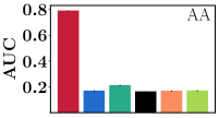
(a)

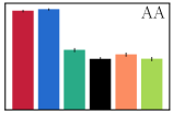
(b)

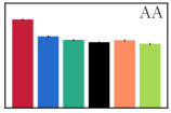
(c)

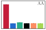
(d)

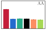
(e)

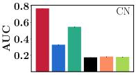
(f)

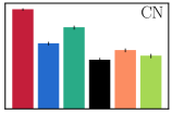
(g)

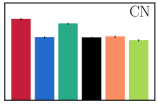
(h)

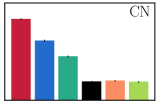
(i)

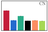
(j)

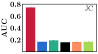
(k)

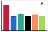
(l)

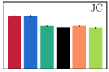
(m)

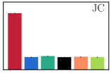
(n)

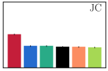
(o)

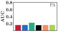
(b) Facebook

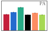
(c) USAir

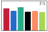
(d) Twitter

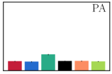
(e) Yeast

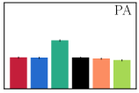
(f) PB

Figure 5: Performance (AUC) on Facebook, USAir, Twitter, Yeast, PB datasets using various DP protocols: DpLp, DpLp-UMNN, DpLp-Lin, Staircase, Laplace and Exponential for 20% held-out set with $\epsilon_{p}=0.1$ and $K=30$ for triad based LP protocols (AA, CN, JC, PA). DpLp outperforms all the baselines in all cases, except preferential attachment, where DpLp-Lin turns out be the consistent winner.

15.1 Results on triad based LP protocols

Here, we first compare the predictive performance of DpLp against its two variants (DpLp-UMNN and DpLp-Lin) and three state-of-the-art baselines (Staircase, Laplace and Exponential) for 20% held-out set with $\epsilon_{p}=0.1$ and $K=30$ for triad based LP protocols across all datasets. Figure 5 summarizes the results, which shows that DpLp outperforms all the baselines in all cases, except preferential attachment, where DpLp-Lin turns out be the consistent winner.

15.2 Results on deep embedding based LP protocols

Next, we compare the predictive performance of DpLp against its two variants (DpLp-UMNN and DpLp-Lin) and three state-of-the-art baselines (Staircase, Laplace and Exponential) for 20% held-out set with $\epsilon_{p}=0.1$ and $K=30$, for deep embedding based LP protocols across all datasets. Figure 6 summarizes the results, which shows that DpLp outperforms the baselines in majority of the embedding methods. For our data sets, we observed that deep node embedding approaches generally fell short of traditional triad-based heuristics. We believe iterated neighborhood pooling already introduces sufficient noise that relaxing $\epsilon_{p}$ does not help these node embedding methods.

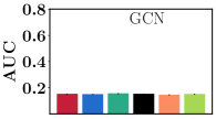
(a)

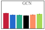
(b)

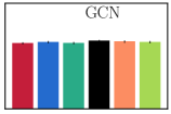
(c)

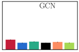
(d)

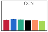
(e)

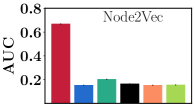
(f)

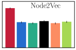
(g)

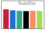
(h)

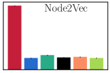
(i)

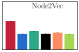
(j)

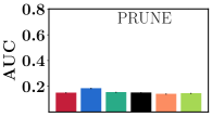
(k)

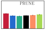
(l)

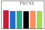
(m)

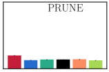
(n)

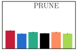
(o)

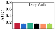
(p)

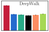
(q)

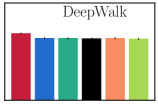
(r)

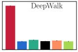
(s)

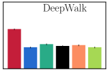
(t)

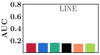
(u)

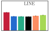
(v)

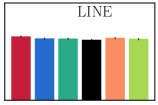
(w)

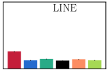
(x)

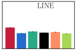
(y)

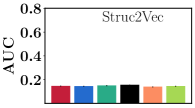
(b) Facebook

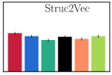
(c) USAir

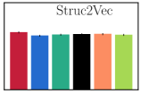
(d) Twitter

(e) Yeast

(f) PB

Figure 6: Performance (AUC) on Facebook, USAir, Twitter, Yeast, PB datasets for various DP algorithms: DpLp, DpLp-UMNN, DpLp-Lin, Staircase, Laplace and Exponential for 20% held-out set with $\epsilon_{p}=0.1$ and $K=30$ for deep embedding based LP protocols (GCN, Node2Vec, PRUNE, DeepWalk, LINE, Struc2Vec). DpLp outperforms the baselines in majority of the embedding methods. However, DP deep methods generally offer worse ranking utility than DP triad-based methods.

References

• Abadi et al. [2016] M. Abadi, A. Chu, I. Goodfellow, H. B. McMahan, I. Mironov, K. Talwar, and L. Zhang. Deep learning with differential privacy. In Proceedings of the 2016 ACM SIGSAC Conference on Computer and Communications Security, pages 308–318, 2016.
• Ackland et al. [2005] R. Ackland et al. Mapping the us political blogosphere: Are conservative bloggers more prominent? In BlogTalk Downunder 2005 Conference, Sydney. BlogTalk Downunder 2005 Conference, Sydney, 2005.
• Backstrom and Leskovec [2011] L. Backstrom and J. Leskovec. Supervised random walks: predicting and recommending links in social networks. In WSDM Conference, pages 635–644, 2011. URL http://cs.stanford.edu/people/jure/pubs/linkpred-wsdm11.pdf.
• Backstrom et al. [2007] L. Backstrom, C. Dwork, and J. Kleinberg. Wherefore art thou r3579x?: anonymized social networks, hidden patterns, and structural steganography. In WWW, 2007.
• Barabási and Albert [1999] A.-L. Barabási and R. Albert. Emergence of scaling in random networks. science, 286(5439):509–512, 1999.
• Batagelj and Mrvar [2006] V. Batagelj and A. Mrvar. Usair dataset, 2006.
• Borgs et al. [2015] C. Borgs, J. Chayes, and A. Smith. Private graphon estimation for sparse graphs. In NeurIPS, 2015.
• Chierichetti et al. [2015] F. Chierichetti, A. Epasto, R. Kumar, S. Lattanzi, and V. Mirrokni. Efficient algorithms for public-private social networks. In SIGKDD, 2015.
• De et al. [2013] A. De, N. Ganguly, and S. Chakrabarti. Discriminative link prediction using local links, node features and community structure. In ICDM, pages 1009–1018. IEEE, 2013.
• Durfee and Rogers [2019] D. Durfee and R. M. Rogers. Practical differentially private top-k selection with pay-what-you-get composition. In Advances in Neural Information Processing Systems, pages 3527–3537, 2019.
• Dwork [2011] C. Dwork. Differential privacy. Encyclopedia of Cryptography and Security, pages 338–340, 2011.
• Dwork and Roth [2014] C. Dwork and A. Roth. The algorithmic foundations of differential privacy. Foundations and Trends in Theoretical Computer Science, 9(3–4):211–407, 2014.
• Fan et al. [2008] R.-E. Fan, K.-W. Chang, C.-J. Hsieh, X.-R. Wang, and C.-J. Lin. Liblinear: A library for large linear classification. JMLR, 2008.
• Gao and Zhou [2015] W. Gao and Z.-H. Zhou. On the consistency of auc pairwise optimization. In Twenty-Fourth International Joint Conference on Artificial Intelligence, 2015.
• Geng and Viswanath [2015] Q. Geng and P. Viswanath. The optimal noise-adding mechanism in differential privacy. IEEE Transactions on Information Theory, 62(2):925–951, 2015.
• Geng et al. [2018] Q. Geng, W. Ding, R. Guo, and S. Kumar. Optimal noise-adding mechanism in additive differential privacy. arXiv preprint arXiv:1809.10224, 2018.
• Ghosh et al. [2012] A. Ghosh, T. Roughgarden, and M. Sundararajan. Universally utility-maximizing privacy mechanisms. SIAM Journal on Computing, 41(6):1673–1693, 2012.
• Grover and Leskovec [2016] A. Grover and J. Leskovec. node2vec: Scalable feature learning for networks. In SIGKDD, 2016.
• Hay et al. [2009] M. Hay, C. Li, G. Miklau, and D. Jensen. Accurate estimation of the degree distribution of private networks. In 2009 Ninth IEEE International Conference on Data Mining, pages 169–178. IEEE, 2009.
• He et al. [2014] X. He, A. Machanavajjhala, and B. Ding. Blowfish privacy: Tuning privacy-utility trade-offs using policies. In Proceedings of the 2014 ACM SIGMOD international conference on Management of data, pages 1447–1458, 2014.
• Hoff et al. [2002] P. D. Hoff, A. E. Raftery, and M. S. Handcock. Latent space approaches to social network analysis. Journal of the American Statistical Association, 97(460):1090–1098, 2002.
• Joachims [2005] T. Joachims. A support vector method for multivariate performance measures. In ICML, 2005.
• Kasiviswanathan et al. [2013] S. P. Kasiviswanathan, K. Nissim, S. Raskhodnikova, and A. Smith. Analyzing graphs with node differential privacy. In Theory of Cryptography Conference, pages 457–476. Springer, 2013.
• Kearns et al. [2015] M. Kearns, A. Roth, Z. S. Wu, and G. Yaroslavtsev. Privacy for the protected (only). arXiv preprint arXiv:1506.00242, 2015.
• Kifer and Machanavajjhala [2014] D. Kifer and A. Machanavajjhala. Pufferfish: A framework for mathematical privacy definitions. ACM Transactions on Database Systems (TODS), 39(1):1–36, 2014.
• Kipf and Welling [2016] T. N. Kipf and M. Welling. Semi-supervised classification with graph convolutional networks. arXiv preprint arXiv:1609.02907, 2016.
• Lai et al. [2017] Y.-A. Lai, C.-C. Hsu, W. H. Chen, M.-Y. Yeh, and S.-D. Lin. PRUNE: Preserving proximity and global ranking for network embedding. In NeurIPS, pages 5257–5266, 2017.
• Leskovec and Mcauley [2012] J. Leskovec and J. J. Mcauley. Learning to discover social circles in ego networks. In NeuIPS, 2012.
• Leskovec et al. [2010] J. Leskovec, D. Chakrabarti, J. Kleinberg, C. Faloutsos, and Z. Ghahramani. Kronecker graphs: An approach to modeling networks. Journal of Machine Learning Research, 11(Feb):985–1042, 2010.
• Liben-Nowell and Kleinberg [2007] D. Liben-Nowell and J. Kleinberg. The link-prediction problem for social networks. Journal of the American Society for Information Science and Technology, 58(7):1019–1031, 2007. ISSN 1532-2890. doi: 10.1002/asi.20591. URL https://onlinelibrary.wiley.com/doi/full/10.1002/asi.20591.
• Liu [2009] T.-Y. Liu. Learning to rank for information retrieval. In Foundations and Trends in Information Retrieval, volume 3, pages 225–331. Now Publishers, 2009. doi: http:/dx.doi.org/10.1561/1500000016. URL http://www.nowpublishers.com/product.aspx?product=INR&doi=1500000016.
• Lü and Zhou [2011] L. Lü and T. Zhou. Link prediction in complex networks: A survey. Physica A: statistical mechanics and its applications, 390(6):1150–1170, 2011. URL https://www.sciencedirect.com/science/article/pii/S037843711000991X.
• Machanavajjhala et al. [2011] A. Machanavajjhala, A. Korolova, and A. D. Sarma. Personalized social recommendations - accurate or private? In VLDB, 2011.
• Marbach and Tsitsiklis [2003] P. Marbach and J. N. Tsitsiklis. Approximate gradient methods in policy-space optimization of markov reward processes. Discrete Event Dynamic Systems, 13(1-2):111–148, 2003.
• Maurer and Pontil [2009] A. Maurer and M. Pontil. Empirical bernstein bounds and sample variance penalization. arXiv preprint arXiv:0907.3740, 2009.
• McSherry and Talwar [2007] F. McSherry and K. Talwar. Mechanism design via differential privacy. In FOCS, pages 94–103, 2007.
• News [2019] News. Report door article. In https://bit.ly/2A5R3kS, 2019.
• News [2020] News. Forbes article, 2020.
• Nissim et al. [2007] K. Nissim, S. Raskhodnikova, and A. Smith. Smooth sensitivity and sampling in private data analysis. In Proceedings of the thirty-ninth annual ACM symposium on Theory of computing, pages 75–84, 2007.
• Perozzi et al. [2014] B. Perozzi, R. Al-Rfou, and S. Skiena. Deepwalk: Online learning of social representations. In KDD, pages 701–710, 2014.
• Peters and Schaal [2006] J. Peters and S. Schaal. Policy gradient methods for robotics. In 2006 IEEE/RSJ International Conference on Intelligent Robots and Systems, pages 2219–2225. IEEE, 2006.
• Ribeiro et al. [2017] L. F. Ribeiro, P. H. Saverese, and D. R. Figueiredo. struc2vec: Learning node representations from structural identity. In SIGKDD Conference, pages 385–394, 2017.
• Sarkar et al. [2011] P. Sarkar, D. Chakrabarti, and A. W. Moore. Theoretical justification of popular link prediction heuristics. In COLT, 2011.
• Sehnke et al. [2010] F. Sehnke, C. Osendorfer, T. Rückstieß, A. Graves, J. Peters, and J. Schmidhuber. Parameter-exploring policy gradients. Neural Networks, 23(4):551–559, 2010.
• Song and Chaudhuri [2017] S. Song and K. Chaudhuri. Composition properties of inferential privacy for time-series data. In 2017 55th Annual Allerton Conference on Communication, Control, and Computing (Allerton), pages 814–821. IEEE, 2017.
• Song et al. [2017] S. Song, Y. Wang, and K. Chaudhuri. Pufferfish privacy mechanisms for correlated data. In Proceedings of the 2017 ACM International Conference on Management of Data, pages 1291–1306, 2017.
• Song et al. [2018] S. Song, S. Little, S. Mehta, S. Vinterbo, and K. Chaudhuri. Differentially private continual release of graph statistics. arXiv preprint arXiv:1809.02575, 2018.
• Tang et al. [2015] J. Tang, M. Qu, M. Wang, M. Zhang, J. Yan, and Q. Mei. LINE: Large-scale information network embedding. In WWW Conference, pages 1067–1077, 2015.
• Tucker [2014] C. E. Tucker. Social networks, personalized advertising, and privacy controls. Journal of Marketing Research, 51(5):546–562, 2014. doi: 10.1509/jmr.10.0355.
• Von Mering et al. [2002] C. Von Mering, R. Krause, B. Snel, M. Cornell, S. G. Oliver, S. Fields, and P. Bork. Comparative assessment of large-scale data sets of protein–protein interactions. Nature, 417(6887):399, 2002.
• Waniek et al. [2019] M. Waniek, K. Zhou, Y. Vorobeychik, E. Moro, T. P. Michalak, and T. Rahwan. How to hide one’s relationships from link prediction algorithms. Scientific reports, 9(1):1–10, 2019.
• Wehenkel and Louppe [2019] A. Wehenkel and G. Louppe. Unconstrained monotonic neural networks. In Advances in Neural Information Processing Systems, pages 1543–1553, 2019.
• Xu et al. [2018] D. Xu, S. Yuan, X. Wu, and H. Phan. Dpne: differentially private network embedding. In Pacific-Asia Conference on Knowledge Discovery and Data Mining, pages 235–246. Springer, 2018.
• Zhang and Chen [2018] M. Zhang and Y. Chen. Link prediction based on graph neural networks. In NeurIPS, 2018.
• Zhao et al. [2011] T. Zhao, H. Hachiya, G. Niu, and M. Sugiyama. Analysis and improvement of policy gradient estimation. In Advances in Neural Information Processing Systems, pages 262–270, 2011.