Scrambled Mean Field Approach to the Quantum Dynamics of Degenerate Bose Gases

Abstract

We present a novel approach to modeling dynamics of trapped, degenerate, weakly interacting Bose gases beyond the mean field limit. We transform a many-body problem to the interaction representation with respect to a suitably chosen part of the Hamiltonian and only then apply a multimode coherent-state ansatz. The obtained equations are almost as simple as the Gross–Pitaevskii equation, but our approach captures essential features of the quantum dynamics such as the collapse of coherence.

The mean-field approximation has become a powerful tool for modeling dynamics of degenerate gases of weakly interacting bosonic atoms Dalfovo ; ufn98 ; Leggett-rev . In this approximation, a Bose–Einstein condensate (BEC) or, in a case of low-dimensional geometry, a quasicondensate is described by a complex-valued classical field subject to the time-dependent Gross-Pitaevskii equation (GPE). Thermal and even quantum zero-point fluctuations can be incorporated into this classical-field picture within the truncated Wigner approximation (TWA) TWA1 via initial conditions. Unfortunately, the TWA with quantum noise provides physically meaningful solutions on rather a restricted time scale TWA2 . An alternative to the mean-field calculations is given by the quantum Boltzmann equation that can be derived by the standard techniques of the non-equilibrium quantum field theory Gasenzer1 ; Werner ; Gasenzer2 . Buchhold and Diehl DiehlEPJD derived kinetic equations not only for populations, but also for anomalous correlations in phonon modes in one dimension (1D). However, the quantum field theory methods are developed for a bulk medium in the thermodynamic limit, where the excitation spectrum is continuous and on-shell self-energies have therefore a non-zero imaginary part. In experiment, the finite size of trapped ultracold atomic clouds makes their excitation spectra discrete with frequencies of different excitation modes being well resolvable Jin96 ; Mewes96 . The multiconfigurational time-dependent Hartree method for bosons (MCTDHB) Alon08 is suitable for numerical modeling the non-mean-field dynamics of finite-size systems. However, it seems that the MCTDHB well describes the experimental data only in situations where the number of involved configurations remains small because of limitations specific for a given process, such as parametric excitation of a Bose–Einstein condensate (BEC) Hulet19 , and remains otherwise suitable mainly for few-body problems. A recently developed truncated conformal space approach Takacs2 ; Takacs1 works well at relatively low excitation energies of a bosonic system, as numerical diagonalization methods in general do.

Experiments with ultracold bosonic gases exhibiting effects beyond the mean field include, first of all, observations of the collapse and revival dynamics in optical lattices Bloch1 ; Bloch2 . Moreover, redistribution of atomic population between lattice sites accompanying this phenomenon has been detected in a recent experiment Zhou . The available theory phase-diff ; Imamoglu-theor ; Kuklov does not account for multimode aspects of the problem and remains a matter-wave analog of the well-known Jaynes–Cummings model in quantum optics cum-collapse ; eber-collapse .

The multimode approach that we present here can be called a scrambled mean field method. It bears certain similarities to the rotated Hartree method Cederbaum87 , but is remarkably simpler. Consider a Hamiltonian $\hat{H}=\hat{H}_{\mathrm{h}}+\hat{H}_{\mathrm{a}}$ that describes a BEC or a low-dimensional quasicondensate in collective variables Dalfovo ; ufn98 ; Leggett-rev . Its harmonic part, $\hat{H}_{\mathrm{h}}$, can be written after diagonalization as $\hat{H}_{\mathrm{h}}=\hbar\sum_{j}\omega_{j}\hat{b}_{j}^{\dagger}\hat{b}_{j}$, where $\hat{b}_{j}^{\dagger}$ and $\hat{b}_{j}$ are the creation and annihilation operators, respectively, of excitation quanta in the $j$th elementary mode with the fundamental frequency $\omega_{j}$ ($\hat{b}_{j}^{\dagger}$ and $\hat{b}_{j}$ obey the standard bosonic commutation rules). We denote the eigenstates of $\hat{H}_{\mathrm{h}}$, i.e., Fock states of elementary excitations, by $|\mathbf{n}\rangle=|\{n_{1},\,n_{2},\,n_{3},\,\dots\}\rangle$, where $\hat{b}_{j}^{\dagger}\hat{b}_{j}|\mathbf{n}\rangle=n_{j}|\mathbf{n}\rangle$. The anharmonic part $\hat{H}_{\mathrm{a}}$ of the Hamiltonian describes interaction between elementary excitations. This interaction is assumed to be small in order to make elementary excitations well defined. Usually $\hat{H}_{\mathrm{a}}$ can be expanded in Taylor series in $\hat{b}_{j}^{\dagger}$ and $\hat{b}_{j}$ beginning from a cubic term in a general case. The first-order perturbative correction to the energy of the state $|\mathbf{n}\rangle$ is given by the matrix element $\langle\mathbf{n}|\hat{H}_{\mathrm{a}}|\mathbf{n}\rangle$. The lowest order term that contributes to $\langle\mathbf{n}|\hat{H}_{\mathrm{a}}|\mathbf{n}\rangle$ is a quartic one, more precisely, its diagonal part $\hat{H}_{\mathrm{qd}}=\frac{\hbar}{2}\sum_{j,j^{\prime}}g_{jj^{\prime}}\hat{b}^{\dagger}_{j}\hat{b}^{\dagger}_{j^{\prime}}\hat{b}_{j^{\prime}}\hat{b}_{j}$, so that $\langle\mathbf{n}|\hat{H}_{\mathrm{a}}|\mathbf{n}\rangle=\frac{\hbar}{2}\sum_{j,j^{\prime}}g_{jj^{\prime}}n_{j}(n_{j^{\prime}}-\delta_{jj^{\prime}})+\Delta E_{\mathbf{n}}$, where $\Delta E_{\mathbf{n}}$ is the contribution of higher-order terms and $g_{jj^{\prime}}=g_{j^{\prime}j}$.

Now we need to introduce a unitary operator that induces quantum correlations between the modes. In contrast to Ref. Cederbaum87 , it contains no time-dependent parameters to be determined from the variational principle, but we derive instead its form from the perturbation theory considerations. We rearrange the terms in the Hamiltonian as $\hat{H}=\hat{H}_{0}+\hat{V}$, where $\hat{H}_{0}=\hat{H}_{\mathrm{h}}+\hat{H}_{\mathrm{qd}}$ and $\hat{V}=\hat{H}_{\mathrm{a}}-\hat{H}_{\mathrm{qd}}$. The evolution of the wave function $|\Psi\rangle$ os the system is governed by the Schrödinger equation $i\hbar\frac{\partial}{\partial t}|\Psi\rangle=\hat{H}|\Psi\rangle$. Our first step is to introduce the interaction representation with respect to the diagonalizable anharmonic Hamiltonian $\hat{H}_{0}$. This is done by an unitary transformation $|\Psi\rangle=\hat{U}_{\mathrm{r}}(t)|\tilde{\Psi}\rangle$, where $\hat{U}_{\mathrm{r}}(t)=\exp(-i\hat{H}_{0}t/\hbar)$. This transformation does not mix different Fock states of elementary excitations, but induces correlations between modes via the energy shift for elementary excitations depending on the quantum state of all the other modes and hence “scrambles” $|\tilde{\Psi}\rangle$. After this transformation the Schrödinger equation reads as

$$i\hbar\frac{\partial}{\partial t}|\tilde{\Psi}\rangle=\hat{\tilde{V}}(t)|\tilde{\Psi}\rangle,$$ (1)

where

$$\hat{\tilde{V}}(t)=\hat{U}_{\mathrm{r}}^{-1}(t)\hat{V}\hat{U}_{\mathrm{r}}(t).$$ (2)

The field operators for the modes transform as

$$\hat{U}_{\mathrm{r}}^{-1}(t)\hat{b}_{j}\hat{U}_{\mathrm{r}}(t)=\hat{\cal A}_{j}\hat{b}_{j},~{}~{}~{}\hat{U}_{\mathrm{r}}^{-1}(t)\hat{b}_{j}^{\dagger}\hat{U}_{\mathrm{r}}(t)=\hat{b}_{j}^{\dagger}\hat{\cal A}_{j}^{\dagger},$$ (3)

$$\hat{\cal A}_{j}=\exp\bigg{(}-i\omega_{j}t-i\sum_{j^{\prime}}g_{jj^{\prime}}\hat{b}^{\dagger}_{j^{\prime}}\hat{b}_{j^{\prime}}t\bigg{)}.~{}$$ (4)

Eqs. (3, 4) allow us to write $\hat{\tilde{V}}$ in explicit form.

We assume that initially, at $t=0$, the state of the system is a product of coherent states (normalized to unity eigenstates of the respective annihilation operators Glauber ) for each mode. This type of initial conditions is also assumed in the mean field theory. Now we make the variational ansatz in the coherent state form not for $|\Psi\rangle$, but for the wave function in the interaction representation:

$$|\tilde{\Psi}\rangle=\prod_{j}\left[e^{-|\psi_{j}|^{2}/2}\sum_{n_{j}=0}^{\infty}\frac{(\psi_{j}\hat{b}_{j}^{\dagger})^{n_{j}}}{n_{j}!}\right]|\mathbf{0}\rangle,$$ (5)

where $|\mathbf{0}\rangle$ is the vacuum state for all the modes. By minimizing the action ${\cal S}=\int dt\,\langle\tilde{\Psi}|\left(i\hbar\frac{\partial}{\partial t}-\hat{\tilde{V}}\right)|\tilde{\Psi}\rangle$ we obtain the evolution equations for the complex functions $\psi_{j}(t)$ parametrizing the coherent states in Eq. (5):

$$i\hbar\frac{\partial}{\partial t}\psi_{j}=\frac{\partial}{\partial\psi_{j}^{*}}\langle\tilde{\Psi}|\hat{\tilde{V}}(t)|\tilde{\Psi}\rangle.$$ (6)

To give a recipe for the calculation of $\langle\tilde{\Psi}|\hat{\tilde{V}}|\tilde{\Psi}\rangle$, we assume that $\hat{V}$ can be expanded in Taylor series in creation and annihilation operators and consider a term $\hat{V}^{j_{1}\dots j_{l}}_{j^{\prime}_{1}\dots j^{\prime}_{l^{\prime}}}=h^{j_{1}\dots j_{l}}_{j^{\prime}_{1}\dots j^{\prime}_{l^{\prime}}}\prod_{\kappa=1}^{l}\hat{b}_{j_{\kappa}}^{\dagger}\prod_{\kappa^{\prime}=1}^{l^{\prime}}\hat{b}_{j^{\prime}_{\kappa^{\prime}}}$, where $h^{j_{1}\dots j_{l}}_{j^{\prime}_{1}\dots j^{\prime}_{l^{\prime}}}$ is a constant. A straightforward calculation based on elementary properties of coherent states yields

$$\langle\tilde{\Psi}|\hat{\tilde{V}}^{j_{1}\dots j_{l}}_{j^{\prime}_{1}\dots j^{\prime}_{l^{\prime}}}|\tilde{\Psi}\rangle \equiv \langle\tilde{\Psi}|\hat{U}_{\mathrm{r}}^{-1}(t)\hat{V}^{j_{1}\dots j_{l}}_{j^{\prime}_{1}\dots j^{\prime}_{l^{\prime}}}\hat{U}_{\mathrm{r}}(t)|\tilde{\Psi}\rangle$$ (7)

$$= h^{j_{1}\dots j_{l}}_{j^{\prime}_{1}\dots j^{\prime}_{l^{\prime}}}\prod_{\kappa=1}^{l}\psi_{j_{\kappa}}^{*}\prod_{\kappa^{\prime}=1}^{l^{\prime}}\psi_{j^{\prime}_{\kappa^{\prime}}}e^{i\nu^{j_{1}\dots j_{l}}_{j^{\prime}_{1}\dots j^{\prime}_{l^{\prime}}}t}\times$$

$$\exp\bigg{[}\!-\sum_{j}|\psi_{j}|^{2}\Big{(}1-e^{iG^{j_{1}\dots j_{l}}_{j^{\prime}_{1}\dots j^{\prime}_{l^{\prime}};j}t}\Big{)}\bigg{]},~{}~{}~{}~{}$$

where

$$\nu^{j_{1}\dots j_{l}}_{j^{\prime}_{1}\dots j^{\prime}_{l^{\prime}}} = \sum_{\kappa=1}^{l}\bigg{(}\omega_{j_{\kappa}}+\sum_{\lambda=\kappa+1}^{l}g_{\kappa\lambda}\bigg{)}-$$ (8)

$$\sum_{\kappa^{\prime}=1}^{l^{\prime}}\bigg{(}\omega_{j_{\kappa^{\prime}}^{\prime}}+\sum_{\lambda^{\prime}=\kappa^{\prime}+1}^{l^{\prime}}g_{\kappa^{\prime}\lambda^{\prime}}\bigg{)},$$

$$G^{j_{1}\dots j_{l}}_{j^{\prime}_{1}\dots j^{\prime}_{l^{\prime}};j} = \sum_{\kappa=1}^{l}g_{jj_{\kappa}}-\sum_{\kappa^{\prime}=1}^{l^{\prime}}g_{jj_{\kappa^{\prime}}^{\prime}}.$$ (9)

The number of the system modes to be taken into account is to be determined in each particular case from physics considerations. A good guidance can be obtained from the thermalization argument. We calculate the mean energy $E=\langle\Psi|\hat{H}|\Psi\rangle$ at $t=0$, assume that the system equilibrates at $t\rightarrow\infty$, and calculate the temperature that corresponds to the internal energy $E$ (if the total number of elementary excitation is conserved, we need to determine also the chemical potential). The number of modes with the mean number of quanta larger than 1 at thermal equilibrium will give an estimation for the minimal number of modes to be considered.

After solving Eq. (6) with the initial conditions $\psi_{j}(0)=\psi_{0j}$, we can the find quantum-mechanical expectation value $\langle\hat{\cal O}\rangle\equiv\langle\Psi|\hat{\cal O}|\Psi\rangle$ for any observable $\hat{\cal O}$ as a function of time. For example, $\langle\hat{b}_{j}+\hat{b}_{j}^{\dagger}\rangle=\psi_{j}\exp\{-i\omega_{j}t-\sum_{j^{\prime}}|\psi_{j^{\prime}}|^{2}[1-\exp(ig_{jj^{\prime}}t)]\}+\mathrm{c.c.}\,$.

We test our method on the Hamiltonian of a two-dimensional (2D) harmonic oscillator with a quartic perturbation:

$$\hat{H} = \hbar\omega_{0}\bigg{[}\frac{1}{2}\left(-\frac{\partial^{2}}{\partial x^{2}}-\frac{\partial^{2}}{\partial y^{2}}+x^{2}+\eta^{2}y^{2}\right)+$$ (10)

$$\alpha_{xx}x^{4}+2\alpha_{xy}x^{2}y^{2}+\alpha_{yy}y^{4}\bigg{]}.$$

The co-ordinates $x$ and $y$ in Eq. (10) are dimensionless. Since this Hamiltonian describes only two modes, many its eigenstates $|\Phi_{\lambda}\rangle$ and respective eigenenergies $\epsilon_{\lambda}$ can be found numerically with a high precision up to pretty high values of $\epsilon_{\lambda}$. In Fig. 1 we show the quantum mechanical mean value and variance of $x$ obtained by solving Eq. (6) in compartison with the results directly following from the expansion $|\Psi(t)\rangle=\sum_{\lambda}e^{-i\epsilon_{\lambda}t/\hbar}|\Phi_{\lambda}\rangle\langle\Phi_{\lambda}|\Psi(0)\rangle$. The same data for $y$ as well as the covariance $\mathrm{Cov}\{xy\}=\langle xy\rangle-\langle x\rangle\langle y\rangle$ are shown in Supplemental Material SM . Our numerical method reproduces the behavior of the expectation values and second-order correlations quite well. As the initially coherent wave packet disperses in the anharmonic potential, its regular motion characterized by oscillating expectation values of the co-ordinates is damped and the co-ordinate variances reach their asymptotic values. We tested numerical energy conservation for our method and found $\langle\Psi|\hat{H}|\Psi\rangle$ not exhibiting a systematic drift and deviating from its initial value by 1% at maximum SM .

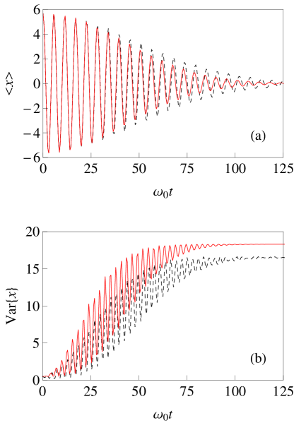
Figure 1: (Color online) (a) The mean value and (b) the variance of the co-ordinate $x$ obtained from the numerical solution of Eq. (6) (red solid line) and from exactly propagated wave function using 1400 lowest eigenstates determined by the numerical diagonalization of Eq. (10) (black dashed line). Values on the axes are dimensionless, the time being scaled by the fundamental frequency $\omega_{0}$. Parameters of the Hamiltonian (10) are: $\eta=1.4$, $\alpha_{xx}=1.9\times 10^{-3}$, $\alpha_{xy}=1.0\times 10^{-3}$, and $\alpha_{yy}=1.1\times 10^{-3}$. The initial coherent state is characterized by $\langle x\rangle=4\sqrt{2}$, $\langle-i\partial/(\partial x)\rangle=0$, $\langle y\rangle=0$, $\langle-i\partial/(\partial y)\rangle=7\sqrt{\eta/2}$ at $t=0$.

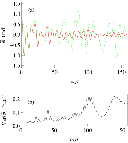
Figure 2: (Color online) (a) Mean global phase difference calculated using the quantum model Eq. (6) with ${\cal M}=21$ modes (red solid line) and the mean field approximation (green dashed line) and (b) its variance according to the quantum model as the function of the dimensionless time $\omega_{\mathrm{J}}t$ for $\hbar\omega_{\|}=3\,{U_{\mathrm{c}}}$ and $\hbar\omega_{\mathrm{J}}=30\,{U_{\mathrm{c}}}$. The initial coherent state corresponds to $\langle\hat{\phi}\rangle=1.5+0.5\sin(\pi s/2)$, $\langle\hat{\rho}\rangle=0$.

We choose the phase difference dynamics in an extended bosonic Josephson junction as the first application of our method to a system with a nontrivially large number of modes. We consider ultracold gas of bosonic atoms in a trap consisting of two tunnel-coupled atomic waveguides, to be referred as the left and right waveguides. The longitudinal trapping is harmonic with the fundamental frequency $\omega_{\|}$. In order to simplify the overview of the example, we make a few approximations. We assume that the number of atoms is small enough to neglect the dependence of the radial width of the atomic cloud on the local density Salasnich , but large enough to provide an inverted parabolic Thomas–Fermi longitudinal profile of the 1D atomic density. Also we consider only antisymmetric modes (out-of-phase motion in the left and right waveguides) and neglect their coupling to the symmetric (in-phase) modes, thus reducing our problem to an ultracold-atom implementation of the sine-Gordon model, but, in contrast to Ref. polk-sg , the mean 1D density profile is in our case non-uniform and proportional to $1-s^{2}$, where $s$ is the dimensionless (scaled to the Thomas–Fermi equilibrium radius $R_{\mathrm{TF}}$) longitudinal co-ordinate. The Hamiltonian reads then

$$\hat{H} = \int_{-1}^{1}ds\,\bigg{[}\frac{U_{\mathrm{c}}}{2}\hat{\rho}^{2}+\frac{\hbar^{2}\omega_{\mathrm{J}}^{2}}{U_{\mathrm{c}}}(1-s^{2})\bigg{(}1-\cos\hat{\phi}\bigg{)}+$$ (11)

$$\frac{\hbar^{2}\omega_{\|}^{2}}{2U_{\mathrm{c}}}(1-s^{2})\bigg{(}\frac{\partial\hat{\phi}}{\partial s}\bigg{)}^{\!2}\,\bigg{]}.$$

Here $\hat{\phi}$ is the operator of the local phase difference between the left and right waveguides, $\hat{\rho}$ is the operator of the conjugate (density-difference) variable. The latter is made dimensionless by scaling to $R_{\mathrm{TF}}^{-1}$, since we use the dimensionless co-ordinate $s$, so that the commutation relation $[\hat{\rho}(s),\hat{\phi}(s^{\prime})]=i\delta(s-s^{\prime})$ holds. The charging energy $U_{\mathrm{c}}$ is positive, since we consider repulsive interactions between atoms. In repulsively interacting quantum gases at low energies the kinetic energy is dominated by phase fluctuations Dalfovo ; ufn98 , therefore we omit a term proportional to $[\partial\hat{\rho}/(\partial s)]^{2}$ in Eq. (11) from the very beginning. The Josephson oscillation frequency corresponding to the peak mean density (at $s=0$) is denoted by $\omega_{\mathrm{J}}$.

In Fig. 2 the results of modeling of the mean and variance of the global phase difference $\bar{\phi}=\frac{1}{2}\int_{-1}^{1}ds\,\hat{\phi}$ are presented (we drop the operator hat above $\bar{\phi}$ to keep notation simple; this observable can be measured by standard experimental techniques Pigneur ). Regular Josephson oscillations decay and the quantum uncertainty of $\bar{\phi}$ becomes large compared to its zero-point level, but still within a range corresponding to high visibility of the integrated interference picture. Their damping of oscillations is not as fast and perfect as in the experiment Pigneur , perhaps, because the model Hamiltonian (11) designed to demonstrate the proof of principle is too simplified.

The numerical method to solve Eq. (6) is overviewed in Supplemental Materials SM . Its most non-trivial part is related to the evaluation of exponential factors appearing in the r.h.s. of Eq. (7). On first glance one may get an impression that, e.g., estimation of a quartic interaction Hamiltonian for ${\cal M}$ modes requires independent calculation of ${\cal O}({\cal M}^{4})$ different terms. However, this “curse of dimensionality” curde can be circumvented in a very efficient way. At times $g_{jj^{\prime}}t\lesssim 1$, which are sufficiently long to observe the collapse of coherence, we can make two simplifications. Firstly, we can neglect the non-commutativity of $\hat{b}_{j}$ and $\hat{\cal A}_{j^{\prime}}$ and, hence, set $\nu^{j_{1}\dots j_{l}}_{j^{\prime}_{1}\dots j^{\prime}_{l^{\prime}}}\approx\sum_{\kappa=1}^{l}\omega_{l}-\sum_{\kappa^{\prime}=1}^{l^{\prime}}\omega_{l^{\prime}}$ [see Eqs. (3,  4,  8)]. Secondly, we can write $\exp[-|\psi_{j}|^{2}(1-e^{iG^{j_{1}\dots j_{l}}_{j^{\prime}_{1}\dots j^{\prime}_{l^{\prime}};j}t})]\approx\exp[i|\psi_{j}|^{2}G^{j_{1}\dots j_{l}}_{j^{\prime}_{1}\dots j^{\prime}_{l^{\prime}};j}t-\frac{1}{2}(|\psi_{j}|G^{j_{1}\dots j_{l}}_{j^{\prime}_{1}\dots j^{\prime}_{l^{\prime}};j}t)^{2}]$, employ the identity $\exp[-\frac{1}{2}(|\psi_{j}|G^{j_{1}\dots j_{l}}_{j^{\prime}_{1}\dots j^{\prime}_{l^{\prime}};j}t)^{2}]=\int_{-\infty}^{\infty}d\sigma\,\exp(i\sigma|\psi_{j}|G^{j_{1}\dots j_{l}}_{j^{\prime}_{1}\dots j^{\prime}_{l^{\prime}};j}t-\frac{1}{2}\sigma^{2})/\sqrt{2\pi}$, and replace the integration by numerical averaging over a normally distributed pseudorandom parameter $\sigma$. These two approximations radically reduce rank of tensors used in numerical evaluation of the r.h.s. of Eq. (6).

To summarize, we developed a novel approach to numerical simulation of the dynamics of finite-size bosonic systems beyond the mean field approximation. Our method is free from the curse of dimensionality and designed to evaluate time scales of the multimode quantum dynamics manifested through the collapse of coherence as well as expectation values and correlations of simple observables. The description of scattering of quanta into initially empty modes remains beyond its scope. The main advantage of our method compared to the multiconfiguration approaches Cederbaum90 ; TC2008 is its remarkable simplicity and numerical efficiency in terms of the computational time and resources; it can be applied to obtain qualitative estimations on such long time scales that the number of configurations needed for the solution by standard methods becomes impractically large. Our method may be used not only in physics of trapped ultracold atomic gases, but also in other fields, such as molecular and chemical physics.

The author thanks C. Lévêque, N. J. Mauser, J.-F. Mennemann, J. Schmiedmayer, and H.-P. Stimming for helpful discussion. This work is supported by the Wiener Wissenschafts- und Technologie Fonds (WWTF) via Grant No. MA16-066 (SEQUEX).

Supplemental Material for

Scrambled Mean Field Approach to the Quantum Dynamics of Degenerate Bose Gases

Igor E. Mazets

Vienna Center for Quantum Science and Technology, Atominstitut, TU Wien,

Stadionallee 2, 1020 Vienna, Austria;

Wolfgang Pauli Institute c/o Fakultät für Mathematik, Universität Wien,

Oskar-Morgenstern-Platz 1, 1090 Vienna, Austria

I. The 2D model

For the 2D Hamiltonian Eq. (10) we introduce

$$\hat{b}_{x} = \frac{1}{\sqrt{2}}\left(x+\frac{\partial}{\partial x}\right),$$

$$\hat{b}_{x}^{\dagger} = \frac{1}{\sqrt{2}}\left(x-\frac{\partial}{\partial x}\right),$$

$$\hat{b}_{y} = \frac{1}{\sqrt{2}}\left(\sqrt{\eta}\,y+\frac{1}{\sqrt{\eta}}\frac{\partial}{\partial y}\right),$$

$$\hat{b}_{y}^{\dagger} = \frac{1}{\sqrt{2}}\left(\sqrt{\eta}\,y-\frac{1}{\sqrt{\eta}}\frac{\partial}{\partial y}\right)$$

and evaluate the r.h.s. of Eq. (6) exactly. The obtained set of two equations for complex functions $\psi_{x}$ and $\psi_{y}$ is solved using a standard package of Wolfram Mathematica 8. The results for the expectation value and the variance of $y$ as well as for the covariance of $x$ and $y$ are plotted below (red solid line). Black dashed line shows the results following from the numerical diagonalization of Eq. (10).

The energy conservation by our scrambled mean-field method is evident from the following ratio of the numerical mean energy $E_{\mathrm{num}}$ to the mean energy $E_{\mathrm{ex}}$ of the initial state calculated from the results of numerically exact diagonalization of Eq. (10):

II. Josephson junction

The harmonic part of the Hamiltonian Eq. (11) is diagonalized by solving the eigenvalue problem

$$\omega_{\mathrm{J}}^{2}(1-s^{2})f_{j}(s)-\omega_{\|}^{2}\frac{d}{ds}\left[(1-s^{2})\frac{df_{j}(s)}{ds}\right]=\omega_{j}^{2}f_{j}(s),$$

with the boundary condition requiring $f_{j}|_{s\rightarrow\pm 1}$ to be finite. The functions $f_{j}(s)$ are real and orthonormalized, $\int_{-1}^{1}ds\,f_{j}(s)f_{j^{\prime}}(s)=\delta_{jj^{\prime}}$. Then the annihilation and creation operators are defined as

$$\hat{b}_{j} = \sqrt{\frac{\hbar\omega_{j}}{2U_{\mathrm{c}}}}\hat{P}_{j}+i\sqrt{\frac{U_{\mathrm{c}}}{2\hbar\omega_{j}}{U_{\mathrm{c}}}}\hat{\Phi}_{j},$$

$$\hat{b}_{j}^{\dagger} = \sqrt{\frac{\hbar\omega_{j}}{2U_{\mathrm{c}}}}\hat{P}_{j}-i\sqrt{\frac{U_{\mathrm{c}}}{2\hbar\omega_{j}}{U_{\mathrm{c}}}}\hat{\Phi}_{j},$$

where $\hat{P}_{j}=\int_{-1}^{1}ds\,f_{j}\hat{\rho}$ and $\hat{\Phi}_{j}=\int_{-1}^{1}ds\,f_{j}\hat{\phi}$.

To simulate numerically the evolution of the anharmonic system in the basis of ${\cal M}=21$ mode, we replaced the integral in Eq. (11) with a sum over ${\cal M}$ Gauss–Legendre quadrature points [1]. This quadrature formula approximates an integral of a function $z(s)$ as $\int_{-1}^{1}ds\,z(s)\approx\sum_{k=1}^{\cal M}w_{k}z(s_{k})$, where $s_{k}$’s are the roots of the Legendre polynomial $P_{{\cal M}}(s)$ and $w_{k}=2/[{\cal M}P_{{\cal M}-1}(s)\frac{d}{ds}P_{{\cal M}}(s)]|_{s=s_{k}}$ are the respective weights. Then Eq. (11) in the ${\cal M}$-mode approximation reads as

$$\hat{H} = \sum_{j=1}^{\cal M}\left(\frac{U_{\mathrm{c}}}{2}\hat{P}_{j}^{2}+\frac{\hbar^{2}\omega_{j}^{2}}{2U_{\mathrm{c}}}\hat{\Phi}_{j}^{2}\right)+$$

$$\frac{\hbar^{2}\omega_{\mathrm{J}}^{2}}{U_{\mathrm{c}}}\sum_{k=1}^{\cal M}w_{k}(1-s_{k}^{2})(1-\frac{1}{2}\hat{\phi}_{k}^{2}-\cos\hat{\phi}_{k}),$$

where the second line represents the anharmonic part $\hat{H}_{\mathrm{a}}$ of the Hamiltonian and $\hat{\phi}_{k}=\sum_{j=1}^{\cal M}f_{j}(s_{k})\hat{\Phi}_{j}$. The coupling constants in $\hat{H}_{\mathrm{qd}}$ are then given by

$$g_{jj^{\prime}}=-\frac{U_{\mathrm{c}}}{4\hbar(1+\delta_{jj^{\prime}})}\frac{\omega_{\mathrm{J}}^{2}}{\omega_{j}\omega_{j}^{\prime}}\sum_{k=1}^{\cal M}w_{k}(1-s_{k}^{2})f_{j}^{2}(s_{k})f_{j^{\prime}}^{2}(s_{k}).$$

As discussed in the main text, on the time scale $t\lesssim\hbar/U_{\mathrm{c}}$ we neglect the anharmonicity-induced corrections (of the order of $U_{\mathrm{c}}/\hbar$) to eigenfrequencies $\omega_{j}$. To the same approximation we neglect the difference between $\hat{H}_{\mathrm{a}}$ and its normally ordered form $:\hat{H}_{\mathrm{a}}:$, where the normal ordering is taken with respect to the creation and annihilation operators of collective excitations (but not of atoms).

Eq. (6) is solved using the second-order predictor-corrector method. The main difficulty is to evaluate $\exp[-|\psi_{j}|^{2}(1-e^{iG^{j_{1}\dots j_{l}}_{j^{\prime}_{1}\dots j^{\prime}_{l^{\prime}};j}t})]\approx\exp[i|\psi_{j}|^{2}G^{j_{1}\dots j_{l}}_{j^{\prime}_{1}\dots j^{\prime}_{l^{\prime}};j}t-\frac{1}{2}(|\psi_{j}|G^{j_{1}\dots j_{l}}_{j^{\prime}_{1}\dots j^{\prime}_{l^{\prime}};j}t)^{2}]$ on each step. As explained in the main text, we use the identity $\exp(-\frac{1}{2}\tau^{2})=\langle e^{i\sigma\tau}\rangle$, where $\langle\dots\rangle$ denotes averaging over Gaussian fluctuations of the random parameter $\sigma$ with zero mean and unity variance. This is implemented as follows. Before starting the numerical propagation in Eq. (6), we prepare the set of real vectors $\sigma^{(j)}_{\gamma}$, $j,\gamma=1,\,2,\,\dots\,,\,{\cal M}$ by generating ${\cal M}$ pseudorandom vectors, orthogonalizing them and imposing normalization $\sum_{\gamma=1}^{\cal M}\sigma^{(j)}_{\gamma}\sigma^{(j^{\prime})}_{\gamma}=\delta_{jj^{\prime}}$. This normalization corresponds to $\langle\sigma^{(j)\,2}_{\gamma}\rangle=1$. The same set of vectors $\sigma^{(j)}_{\gamma}$ is used throughout the numerical propagation of Eq. (6). Each time step of the predictor-corrector scheme is repeated $2{\cal M}$ times with a temporal replacement of $\psi_{j}$ by $\psi_{j}\exp(i\ell\sum_{j^{\prime}}g_{jj^{\prime}}|\psi_{j^{\prime}}|\sigma^{(j^{\prime})}_{\gamma}t)$ with $\gamma$ running from 1 to ${\cal M}$ and $\ell=\pm 1$ and the averaged result determines the values of $\psi_{j}$ at the next grid point of the time axis. Note that taking both signs of $\ell$ provides automatically the equality to zero of the imaginary part of our approximation of Gaussian factors.

Our solution is stable against choosing different sets of $\sigma^{(j)}_{\gamma}$. As we can see from the next plot, the discrepancy $\Delta\bar{\phi}$ between values of the global phase difference $\bar{\phi}$ obtained from two numerical solutions with different choices of $\sigma^{(j)}_{\gamma}$ is of the order of $10^{-2}$ rad.

Our final test shows that the energy is conserved at the accuracy of about 2%, as we can see from comparison of the averaged values of the Hamiltonian $\langle\hat{H}\rangle\equiv\langle\Psi|\hat{H}|\Psi\rangle$ at $t>0$ and $t=0$.

***

[1] D. P. Laurie, J. Comput. Appl. Math. 127, 201 (2001).

References

(1) F. Dalfovo, S. Giorgini, L. P. Pitaevskii, and S. Stringari,
Theory of Bose-Einstein condensation in trapped gases.
Rev. Mod. Phys. 71, 463 (1999).
(2) L. P. Pitaevskii, Bose-Einstein condensation in magnetic traps. Introduction to the theory.
Physics-Uspekhi 41, 569 (1998).
(3) A. J. Leggett, Bose-Einstein condensation in the alkali gases: Some fundamental concepts.
Rev. Mod. Phys. 73, 307 (2001).
(4) M. J. Steel, M. K. Olsen, L. I. Plimak, P. D. Drummond, S. M. Tan, M. J. Collett, D. F. Walls, and R. Graham,
Dynamical quantum noise in trapped Bose-Einstein condensates.
Phys. Rev. A 58, 4824 (1998).
(5) A. Sinatra, C. Lobo, and Y. Castin, The truncated Wigner method for Bose-condensed
gases: limits of validity and applications. J. Phys. B 35, 3599 (2002).
(6) T. Gasenzer, J. Berges, M. G. Schmidt, and M. Seco,
Nonperturbative dynamical many-body theory of a Bose-Einstein condensate.
Phys. Rev. A 72, 063604 (2005).
(7) H. Aoki, N. Tsuji, M. Eckstein, M. Kollar, T. Oka, and P. Werner,
Nonequilibrium dynamical mean-field theory and its applications.
Rev. Mod. Phys. 86, 779 (2014).
(8) I. Chantesana, A. P. Orioli, and T. Gasenzer,
Kinetic theory of nonthermal fixed points in a Bose gas.
Phys. Rev. A 99, 043620 (2019).
(9) M. Buchhold and S. Diehl, Kinetic theory for interacting Luttinger liquids.
Eur. Phys. J. D 69, 224 (2015).
(10) D. S. Jin, J. R. Ensher, M. R. Matthews, C. E. Wieman, and E. A. Cornell,
Collective Excitations of a Bose-Einstein Condensate in a Dilute Gas.
Phys. Rev. Lett. 77, 420 (1996).
(11) M.-O. Mewes, M. R. Andrews, N. J. van Druten, D. M. Kurn, D. S. Durfee, C. G. Townsend, and W. Ketterle,
Collective Excitations of a Bose-Einstein Condensate in a Magnetic Trap.
Phys. Rev. Lett. 77, 988 (1996).
(12) O. E. Alon, A. I. Streltsov, and L. S. Cederbaum,
Multiconfigurational time-dependent Hartree method for bosons: Many-body dynamics of bosonic systems.
Phys. Rev. A 77, 033613 (2008).
(13) J. H. V. Nguyen, M. C. Tsatsos, D. Luo, A. U. J. Lode, G. D. Telles, V. S. Bagnato, and R. G. Hulet,
Parametric Excitation of a Bose-Einstein Condensate: From Faraday Waves to Granulation.
Phys. Rev. X 9, 011052 (2019).
(14) D. X. Horváth and G. Takács, Overlaps after quantum quenches in the sine-Gordon model.
Phys. Lett. B 771, 539 (2017).
(15) I. Kukuljan, S. Sotiriadis, and G. Takacs,
Correlation Functions of the Quantum Sine-Gordon Model in and out of Equilibrium.
Phys. Rev. Lett. 121, 110402 (2018).
(16) M. Greiner, O. Mandel, T. W. Hänsch, and I. Bloch,
Collapse and revival of the matter wave field of a Bose Einstein condensate.
Nature 419, 51 (2002).
(17) S. Will, T. Best, U. Schneider, L. Hackermüller, D.-S. Lühmann,
and I. Bloch, Time-resolved observation of coherent multi-body interactions
in quantum phase revivals. Nature 465, 197 (2010).
(18) T. Zhou, K. Yang, Z. Zhu, X. Yu, S. Yang, W. Xiong, X. Zhou, X. Chen,
C. Li, J. Schmiedmayer, X. Yue, and Y. Zhai,
Observation of atom-number fluctuations in optical lattices via quantum collapse and revival dynamics.
Phys. Rev. A 99, 013602 (2019).
(19) J. Javanainen and M. Wilkens, Phase and Phase Diffusion of a Split Bose-Einstein Condensate.
Phys. Rev. Lett. 78, 4675 (1997).
(20) A. Imamoḡlu, M. Lewenstein, and L. You,
Inhibition of Coherence in Trapped Bose-Einstein Condensates. Phys. Rev. Lett. 78, 2511 (1997).
(21) A. B. Kuklov, N. Chencinski, A. M. Levine, W. M. Schreiber, and J. L. Birman,
Quantum dephasing of normal modes of a Bose-Einstein condensate in a magnetic trap.
Phys. Rev. A 55, R3307(R) (1997).
(22) F. W. Cummings, Stimulated emission of radiation in a single mode.
Phys. Rev. 140, A1051 (1965).
(23) J. H. Eberly, N. B. Narozhny, and J. J. Sanchez-Mondragon,
Periodic spontaneous collapse and revival in a simple quantum model.
Phys. Rev. Lett. 44, 1323 (1980).
(24) J. Kucar, H.-D. Meyer, and L. S. Cederbaum, Time-dependent rotated Hartree approach.
Chem. Phys. Lett. 140, 525 (1987).
(25) R. J. Glauber, Coherent and Incoherent States of the Radiation Field.
Phys. Rev. 131, 2766 (1963).
(26) See Supplemental Material.
(27) L. Salasnich, A. Parola, and L. Reatto,
Effective wave equations for the dynamics of cigar-shaped and disk-shaped Bose condensates.
Phys. Rev. A 65, 043614 (2002).
(28) V. Gritsev, A. Polkovnikov, and E. Demler,
Linear response theory for a pair of coupled one-dimensional condensates of interacting atoms.
Phys. Rev. B, 75, 174511 (2007).
(29) M. Pigneur, T. Berrada, M. Bonneau, T. Schumm, E. Demler, and J. Schmiedmayer,
Relaxation to a Phase-Locked Equilibrium State in a One-Dimensional Bosonic Josephson Junction.
Phys. Rev. Lett. 120, 173601 (2018).
(30) J. F. Traub and A. G. Werschulz, Complexity and information
(Cambridge University Press, Cambridge, 1998).
(31) H.-D. Meyer. U.Manthe, and L. S. Cederbaum,
The multi-configurational time-dependent Hartree approach. Chem. Phys. Lett. 165, 73 (1990).
(32) J. M. Bowman, T. Carrington, and H.-D. Meyer, Variational quantum approaches for computing vibrational
energies of polyatomic molecules. Molecular Phys. 106, 2145 (2008).