A bayesian-like approach to derive chemical abundances in Type-2 Active Galactic Nuclei based on photoionization models

Abstract

We present a new methodology for the analysis of the emission lines of the interstellar medium in the Narrow Line Regions around type-2 Active Galactic Nuclei. Our aim is to provide a recipe that can be used for large samples of objects in a consistent way using different sets of optical emission-lines that takes into the account possible variations from the O/H - N/O relation to use [N ii] lines. Our approach consists of a bayesian-like comparison between certain observed emission-line ratios sensitive to total oxygen abundance, nitrogen-to-oxygen ratio and ionization parameter with the predictions from a large grid of photoionization models calculated under the most usual conditions in this environment. We applied our method to a sample of Seyfert 2 galaxies with optical emission-line fluxes and determinations of their chemical properties from detailed models in the literature. Our results agree within the errors with other results and confirm the high metallicity of the objects of the sample, with N/O values consistent wit a large secondary production of N, but with a large dispersion. The obtained ionization parameters for this sample are much larger than those for star-forming object at the same metallicity.

1 Introduction

Active galactic nuclei (AGNs) are among the most luminous objects in the Universe. The intense and energetic radiation coming from the accretion disk and the jets around supermassive black holes in the centers of galaxies is absorbed by the surrounding interstellar medium (ISM) and partially reemitted as very bright and prominent emission-lines that contain valuable information about the physical conditions, the chemical abundances and the mechanical properties of the gas under these very extreme conditions. Since these objects can be studied up to very high redshifts the correct characterization of this kind of spectra can thus provide information about the cosmic evolution of galaxies.

It is widely accepted from the works by several authors (e.g. Ferland & Netzer 1983; Halpern & Steiner 1983) that, according to models, the main mechanism of ionization in the Narrow Line Region (NLR) in AGNs is photoionization. This can in principle opens the gate to the estimation of the physical properties and the ionic abundances in the gas by the measurement of the most prominent optical emission-lines. However, it is known that the most widely used recipes to derive the total metallicity using this information in star-forming regions (i.e. the $T_{e}$ method) leads to sub-solar metallicities in AGNs, which are very low as compared to the predictions from photoionization models or the expected values for their radial positions in galactic disks (e.g. Dors et al. 2015).

In this way models become a crucial tool to interpret the observed optical and ultraviolet spectra of NLRs and they have been traditionally used to provide calibrations for the derivation of total metallicity from the measurement of the emission lines (e.g. Storchi-Bergmann et al. 1998; Nagao et al. 2006; Dors et al. 2014). Models are also used to derive abundances in star-forming regions, where it is known that the $T_{e}$ method leads to precise abundance estimations. This occurs in the case that the electron temperature cannot be derived because the required auroral lines (e.g. [O iii] $\lambda$4363 Å) is too weak to be measured or owing to a too restricted observed spectral range. Although many authors point out that models can lead to systematically higher oxygen abundances than those calculated using the $T_{e}$ method also in the case of star-forming regions (e.g. Kewley & Dopita 2002; Blanc et al. 2015; Vale Asari et al. 2016), these differences are much lower than in the case of the NLRs of AGNs and are even negligible in some works (e.g. Pérez-Montero et al. 2010; Dors et al. 2011).

Models are also useful to overcome the problem of relative variations between different elemental abundances whose emission-lines are used as tracers of the total metallicity. This is the case of the nitrogen-to-oxygen ratio (N/O), which has a monotonically growing behavior with O/H in the high-metallicity regime (i.e. $Z\geq 0.3\cdot Z_{\odot}$) as predicted by galactic chemical evolution models under the assumption of total isolation, as most of nitrogen production is secondary (Henry et al., 2000). However it is known that hydrodynamical effects can affect the ratio between secondary and primary elemental abundances (Edmunds, 1990), what can cause non-negligible deviations in the derivation of O/H or in the AGN identification using N emission lines such as [N ii] $\lambda$6583 Å (Pérez-Montero & Contini, 2009). This emission-line is especially bright and used in the case of the NLRs and it has been proposed as a direct estimator of the total metallicity from the ratio of its flux with the H$\alpha$ one (e.g. Storchi-Bergmann et al. 1998; Groves et al. 2006) or in relation to the [O ii] $\lambda$3727 Å (Castro et al., 2017), which has a lower dependence on excitation.

In this work we propose a new method based on photoionization models to derive chemical abundances in the NLRs of AGNs, whose validity has been already proved for star-forming regions. The code Hii-Chi-mistry (hereafter HCm, Pérez-Montero 2014) establishes a bayesian-like comparison between the relative observed optical line fluxes emitted by the ionized gas and the predictions from a grid of photoionization models covering a large range of input conditions in O/H, N/O and ionization parameter ($U$). The code, as probed for star-forming regions, has the advantages that i) firstly estimates the N/O ratio as a free parameter so the [N ii] lines can be used as direct tracers of metallicity, ii) it is totally consistent with the predictions from the $T_{e}$ method, even in the absence of any auroral line, and iii) provides consistent solutions regardless of the input emission-lines given to find a solution, what makes this tool especially useful to compare sets of observations with different spectral ranges or redshifts. The use of such a tool in the case of AGNs would allow to provide solutions to the estimation of O/H and N/O for large samples of objects, in an automatic way and supplying uncertainties, that can later be compared with other AGNs or star-forming galaxies in a consistent way.. Similar methodology than the one considered here was recently used by Thomas et al. (2019) and Mignoli et al. (2019)) in order to calculate the metallicity of NLRs of local Seyfert 2 ($z\,\la\,0.3$) and of obscured (type2) AGNs ($1.4\,\la\,z\,\la\,3.0$), respectively.

The paper is organized as follows. In Section 2 we describe the observational sample compiled and analyzed in Dors et al. (2017) and used here to test the accuracy of our method as these objects have previous similar model-based estimations both for O/H and N/O using optical emission lines that can help to quantify the accuracy and uncertainty of our method. In Section 3 we describe the HCm code and the photoionization models to be used as grid of values for it in the specific landscape of the NLRs of type-2 AGNs. In Section 4 we discuss the results obtained from the application of the code to the control sample, the consistency of our method with the $T_{e}$ method and how our results vary as a function of different input parameters in the models, such as the electron density or the shape of the ionizing spectral energy distribution. Finally, in Section 5 we summarize our results and present our conclusions.

2 Description of the control sample

In order to establish comparisons between the predicted abundances from our code with other model-based results in a sample of objects with the required spectral information we resorted to the objects described and analyzed in Dors et al. (2017). This sample consists of 47 Seyfert 1.9 and 2 galaxies at a redshift $z$ ≲0.1 with observations in the optical range covering all the required reddening corrected, relative to H$\beta$emission-line fluxes to be used as an input by the code, including [O ii] $\lambda$3727 Å, [Ne iii] 3868 Å, [O iii] 4363 and 5007 ÅÅ, [N ii] $\lambda$6583 Å, and [S ii] $\lambda$$\lambda$6717,6731 ÅÅ, with a full width half maximum lower than 1 000 km $\cdot$ s^-1.

Despite these lines were measured using different observational techniques and apertures, all of them can be unambiguously attributed to the NLR in each galaxy and thus can be considered as an integrated emission that can be later reproduced in a single photoionization model.

We also used as control sample the abundance estimations derived by Dors et al. (2017). These authors used the Cloudy code to build detailed tailored photoionization models to reproduce observed optical narrow emission line intensities compiled from the literature in order to obtain quantitative determinations of oxygen and nitrogen abundances for a sample of 44 AGNs. These authors found oxygen and nitrogen abundances in the range $0.4-2$ and $0.3-7.5$ times the solar values, respectively, concluding that these galaxies have abundances quite similar to those of high-metallicity extragalactic H ii regions.

The list of reddening corrected emission lines, the control abundances and the names and redshifts of these galaxies can be found in Dors et al. (2017).

3 Description of the method

The strategy followed to derive ionic abundances and ionization parameters described in this paper is rather similar to that described in Pérez-Montero (2014) to obtain these quantities in star-forming H ii regions. The idea is to establish a direct comparison between a grid of photoionization models covering a large range of input properties and a set of reddening-corrected emission lines relative to a recombination Hi line by means of a bayesian-like approach that later provides us with the most probable values and their corresponding uncertainties. This method can be applied to a large number of objects using the same procedure without need of performing detailed modelling of the gas.

3.1 The grid of models

The grid of models used to be compared with a set of observed optical emission lines in type-2 AGNs was calculated by using the code Cloudy v.17.01 (Ferland et al., 2017). This code calculates the emergent spectrum emitted by a spherical gas distribution surrounding a central point-like ionizing source. We assumed that the gas was distributed homogeneously with a filling factor of 0.1 and a constant density of 500 cm^-3, typical in the NLRs around type-2 AGNs (Dors et al., 2014). about the maximum value found by Dors et al. (2014). The Spectral Energy Distribution (SED) was considered to be composed by two components: one representing the Big Blue Bump peaking at 1 Ryd, and the other a power law with spectral index $\alpha_{x}$ = -1 representing the non-thermal X-rays radiation. As usual, the continuum between 2 keV and 2500 Å is described by a power law with a spectral index $\alpha_{ox}$=-0.8. This value represents the highest in the range derived in the sample of radio-intermediate and radio-loud quasars studied by Miller et al. (2011), but it is the most adequate to reproduce [O iii]/H$\beta$ most type-2 AGNs according to Dors et al. (2017). The stopping criterion to measure the resulting emergent spectrum is that the proportion of free electrons in the ionized gas is lower than 98%. We considered a dust-to-gas ratio with the standard Milky Way value. All chemical abundances were scaled to oxygen following the solar proportions given by Asplund et al. (2009), with the exception of nitrogen, that was left as an extra free input parameter in the models.

We have chosen the input parameters in the grid of models according to the most usual conditions observed in the NLRs of AGNs but additional uncertainties are expected in the results when these vary (e.g. density and chemical inhomogeneities, matter-bounded geometry, distribution of dust and sources, atomic data, etc). However, although it is beyond the scope of this paper to discuss in detail the effect of these factors in the derivation of the resulting abundances, in Section 4 we discuss the impact on our results of two of these parameters, as it is the electron density and the $\alpha_{ox}$ parameter as these are two of the main driver factors that can affect the final results (e.g. Dors et al. (2019)). In the first case we also built a grid with a higher electron density of 2 000 cm^-3, and in the second with an $\alpha_{ox}$ = -1.2, which is near the mean value found by Miller et al. (2011). In all case the code here presented admits new and modified grids that can allow us to study other sources of uncertainty in the models.

Overall, the models cover the range of 12+log(O/H) from 6.9 to 9.1 in bins of 0.1 dex. In addition we consider values of log(N/O) from -2.0 to 0.0 in bins of 0.125 dex. Besides all models consider values of log $U$ from -4.0 to -0.5 in bins of 0.25 dex. This implies to extend towards higher values of log $U$ the range originally defined in Pérez-Montero (2014) for star-forming regions as it is expected to find very high values of this parameter in AGNs (e.g. Matsuoka et al. 2018). This gives a total of 5 865 models in the grid. In addition to improve the model resolution as it is discussed for star-forming regions in Pérez-Montero et al. (2016), the code also allows to interpolate linearly the fluxes predicted by the models by a factor 5 in the three running input variables in the grid (i.e. O/H, N/O, and log $U$). We also discuss in Section 4 the impact of the enhancement of the resolution of the grid in the results.

In Figure 1 we show two of the so-called BPT (Baldwin et al., 1981) diagrams, traditionally used to classify star-forming galaxies and AGNs, representing the emission line ratios [O iii]/H$\beta$vs. [N ii]/H$\alpha$  and [O iii]/H$\beta$vs. [S ii]/H$\alpha$ for the control sample as compared with the results of the whole grid of models. As can be seen the objects lie in the right upper region of the diagrams over the separation curves defined by Kauffmann et al. (2003) and Kewley et al. (2001) and most of this sample is well covered by the grid. A large fraction of the models of the grid occupies the region usually assigned to star-forming objects, but this position is apparently controlled by the metallicity of the models, as also discussed in Kewley et al. (2001), so the observed position of Sy2 galaxies in these diagrams is possibly of empirical origin.

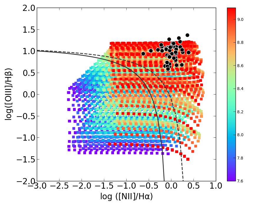
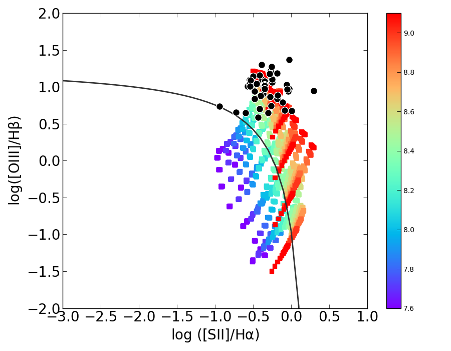
Figure 1: Diagnostic diagrams showing the emission-line ratio [O iii]/H$\beta$ in relation to [N ii]/H$\alpha$ (left) and to [S ii]/H$\alpha$ (right) both for the control sample (black circles) and the whole grid of models (colored squares). The color bar represents the metallicity of each model. The solid line represents the curve defined by Kauffman et al (2003) to separate AGNs and star-forming regions. The dashed red line represents the line defined by Kewley et al (2001) to separate AGNs from pure star-forming and composite regions.

3.2 The HCm code adapted for AGNs

The program HCm was done using python to calculate O/H and N/O chemical abundances ratios and log$U$ using a bayesian-like comparison between the predictions from the models described above and a set of observable emission lines. This code was originally designed to be used in star-forming galaxies but in this work we describe its application and the specific features taken into the account for its use in the NLR of AGNs. The availability of the code ensures its application for large samples of objects and its reproducibility for different samples of objects. At same time it allows to change the library models adapting them to different initial assumptions for the calculation.

The code uses as observable inputs the reddening corrected relative-to-H$\beta$ emission lines from [O ii] $\lambda$3727 Å, [Ne iii] $\lambda$3868 Å,[O iii] $\lambda$4363 Å, [O iii] $\lambda$5007 Å, [N ii] $\lambda$6583 Å, and [S ii] $\lambda$$\lambda$6717+6731 Å with their corresponding errors. However, the code also provides a solution in case one or several of these are not given, what implies that the assumptions made to perform the corresponding calculations and the final derived uncertainty vary accordingly as it is described in the sections below.

3.2.1 Derivation of N/O

In a first iteration the code searches for N/O as a weighted mean over all the space of models: since N/O can be estimated using optical emission-lines of similar excitation, it can be calculated without any specific assumption about the ionization parameter and helps to constrain the space of models to use [N ii] lines to derive oxygen abundance in a second later iteration.

$$\log({\rm N/O})_{f}=\frac{\sum_{i}\log({\rm N/O})_{i}/\chi^{2}_{i}}{\sum_{i}1/\chi^{2}_{i}}$$ (1)

where log(N/O)_f is the final derived nitrogen-to-oxygen ratio, log(N/O)_i are the values for each one of the individual models and the $\chi$ values are assigned for each model as:

$$\chi_{i}=\sum_{j}\frac{(O_{j}-T_{ji})^{2}}{O_{j}}$$ (2)

being the normalized quadratic difference between certain observed emission line ratios, $O_{j}$, and the corresponding prediction from each model, $T_{j}$. The errors are calculated as the quadratic sum of the standard deviation of the $\chi$-weighted resulting distribution and that from a Monte Carlo simulation carried out using the random deviation in each line from the input emission line uncertainties.

In the case of N/O the code uses two different observable sensitive emission-line ratios. Pérez-Montero & Contini (2009) suggested the use of N2O2, defined as:

$${\rm N2O2}=\log\left(\frac{[{\rm N\textsc{ii}}]\lambda 6583}{[{\rm O\textsc{II}}]\lambda 3727}\right),$$ (3)

and a similar version more useful for restricted observed spectral ranges, and hence less sensitive to reddening correction or flux calibration, the N2S2 parameter, defined as:

$${\rm N2S2}=\log\left(\frac{[{\rm N\textsc{ii}}]\lambda 6583}{[{\rm S\textsc{ii}}]\lambda\lambda 6717+6731}\right)$$ (4)

These parameters have the advantage that they do not present almost any dependence on excitation as they only involve low-excitation lines. Indeed they have been proposed for star-forming objects as direct tracers of the metallicity, based on the assumption that secondary production of N at high-metallicity makes N/O to be a direct estimator of O/H. N2O2 has been also proposed as estimator of total metallicity in NLR of Sy2 galaxies by Castro et al. (2017) using results from photoionization models and an assumption about the expected relation between oxygen and nitrogen relative abundances.

In Figure 2 we see the behavior of these two parameters with N/O both from some of the models of the grid and from the estimates obtained by Dors et al. (2017) for the control sample. As it can be seen the models do not show a large dispersion as a function of metallicity or excitation and the objects tend to adopt a linear relation in both cases with N/O. In addition we see that the adopted relations for star-forming objects by Pérez-Montero & Contini (2009) are not valid in the case of NLRs of AGNs and new relations can be adopted for this kind of objects.

In this way, as a sub-product of the models, a linear fitting to them can be used to derive in an alternative direct way the N/O ratio, yielding on one hand, for N2O2:

$$\log({\rm N/O})=(0.97\pm 0.01)\cdot{\rm N2O2}-(0.50\pm 0.01)$$ (5)

which is also represented in Figure 2. The mean offset of the objects analyzed in Dors et al. (2017) is only of 0.07 dex higher with a standard deviation in the residuals of 0.13 dex.

Regarding N2S2, the linear fitting to the whole grid of models gives:

$$\log({\rm N/O})=(0.88\pm 0.01)\cdot{\rm N2S2}-(0.69\pm 0.01)$$ (6)

In this case, the mean offset of the N/O values derived using this expression in relation to values derived by Dors et al. (2017) is 0.05 dex higher with a standard deviation of the residuals of 0.12 dex.

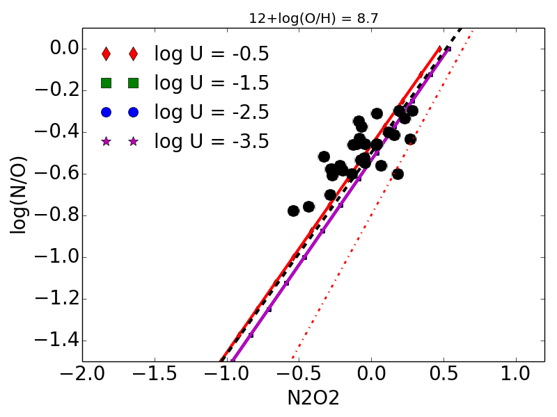
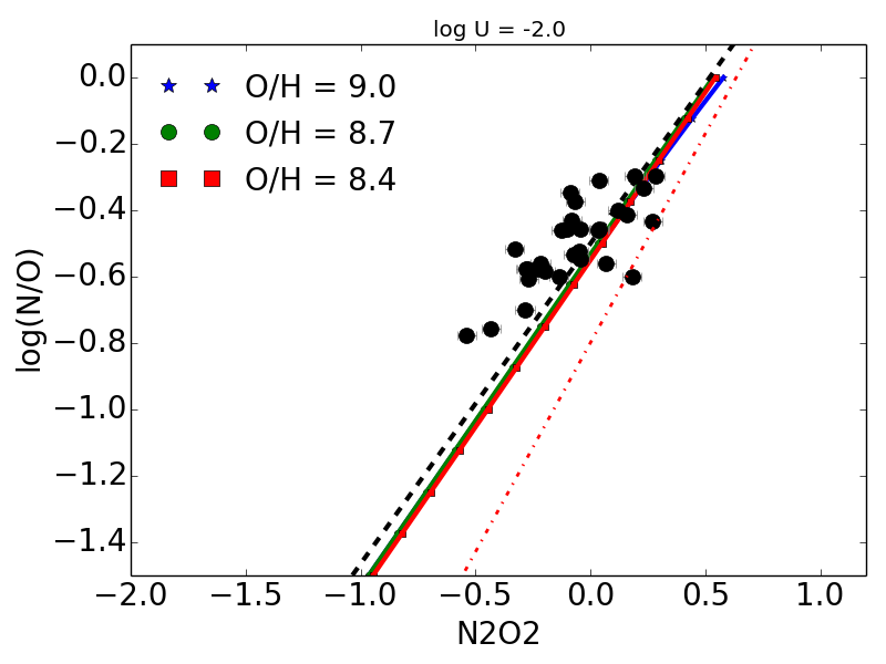
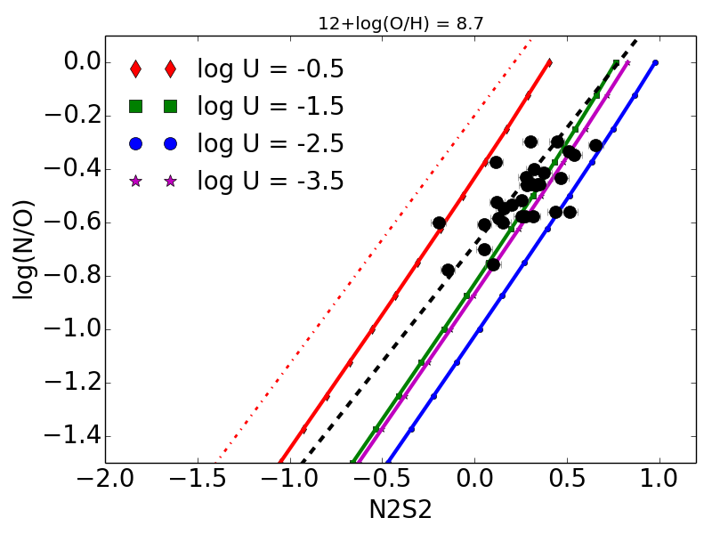
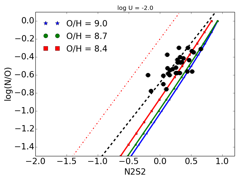
Figure 2: Relation between the elemental abundance ratio N/O with the emission line ratios N2O2 (upper panels) and N2S2 (lower panels) both for some of the models of the grid and for the control sample with the abundances derived by Dors et al (2017). The panels in the left column show results from the models described in the text at a fixed O/H = 8.7 and the panels at right column at a fixed log($U$) = -2.0. The dashed black lines in all panels represent the linear fitting to the models while thered point-dashed lines represent the empirical calibrations of these relations for star-forming objects in Pérez-Montero & Contini (2009).

3.2.2 Derivation of O/H and U

Once N/O has been estimated, the code begins a new iteration through the space of models constrained to the N/O values and the derived uncertainty. The code now calculates the values of the total oxygen abundance and the ionization parameter as the weighted means over all the considered models as:

$$12+\log({\rm O/H})_{f}=\frac{\sum_{i}(12+\log({\rm O/H}))_{i}/\chi^{2}_{i}}{\sum_{i}1/\chi^{2}_{i}}$$ (7)

and

$$\log(U)_{f}=\frac{\sum_{i}\log(U)_{i}/\chi^{2}_{i}}{\sum_{i}1/\chi^{2}_{i}}$$ (8)

where the (O/H)_f and $U_{f}$ are the resulting values, and the (O/H)_i and $U_{i}$ are the individual values for each model. The $\chi^{2}$ values and the corresponding errors are calculated in the same way as it was explained for N/O. We now describe the observables used for the calculation of the $\chi_{i}$ values, including:

$${\rm RO3}=\frac{[{\rm O\textsc{iii}}]\lambda 5007\AA}{[{\rm O\textsc{iii}}]\lambda 4363\AA}$$ (9)

what has a direct relation with the electron temperature of the gas. In NLRs of AGNs the direct relation of this ratio with total oxygen abundance is not well established but, according to models, can be also used as a proxy for the presence of heavy elements in the gas. The main problem in this scenario is that, contrary to star-forming regions, models predict that anon-negligible fraction of the oxygen total abundance correspond to higher ionization stages whose emission lines are not detectable in the optical range. Therefore it is not evident to derive any direct relation between the relative intensities of the strongest optical emission-lines and the total abundances of the elements emitting them.

In Figure 3 we show the relation between the logaritm of this emission-line ratio and the abundances derived by Dors et al. (2017) for the control sample along with some of the models of the grid at a fixed log(N/O) = -0.5.. The models cover the values estimated in these objects, but the direct relation with metallicity is only clear at high values, when the ions of the metals whose lines are observed in the optical range begin to act as effective coolants of the gas and they have a clear influence on its electron temperature, what in star-forming regions occurs at much more lower values of O/H.

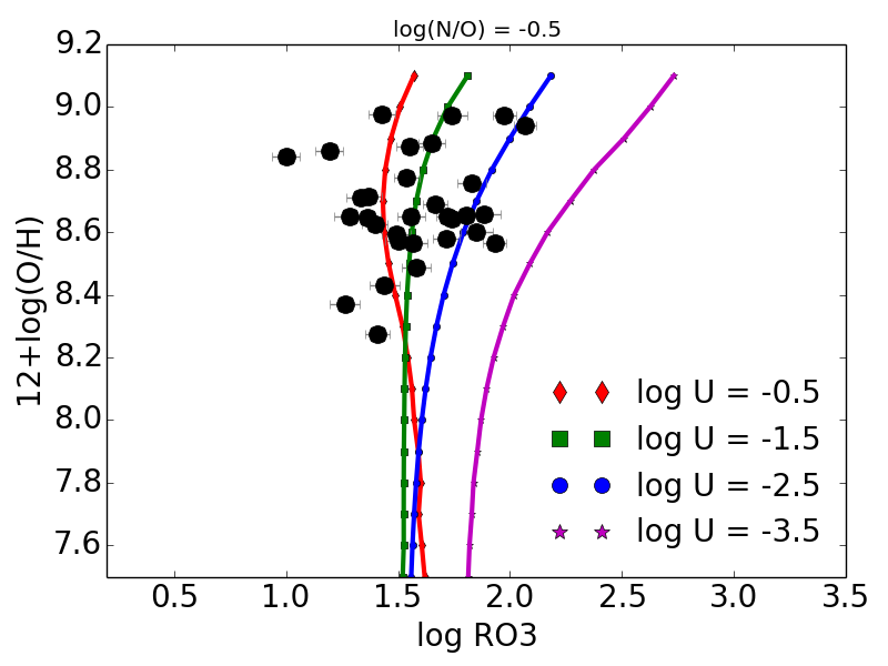
Figure 3: Relation between the total oxygen abundance and the logarythm of the emission line ratio [O iii] $\lambda$$\lambda$5007/4363 Å both for the abundances derived by Dors et al (2017) for the control sample, as represented with black circles, and for models, for different values of $U$, at a fixed log(N/O) value of -0.5.

In relation to other observables used by the code based on nitrogen lines, since N/O has been fixed in the space of models by the code in the previous step described above, the [N ii] emission lines can be now used to derive oxygen abundances. Otherwise, if the studied object lies out of the expected chemical relation between O/H and N/O we can obtain wrong derivations of O/H.

Among the estimators of O/H based on [N ii] used as observables by the code are the N2 parameter (Storchi-Bergmann et al., 1994; Denicoló et al., 2002), defined as:

$${\rm N2}=\log\left(\frac{[{\rm N\textsc{ii}}]\lambda 6583}{H\alpha}\right)$$ (10)

This ratio has the advantage that does not depend on reddening correction and it is easy to measure in the red part of the spectrum with an adequate resolution. This emission-line ratio has been also pointed out as a good tracer of total metallicity in NLRs of AGNs by Storchi-Bergmann et al. (1998), who also point out its relatively lower dependence on ionization parameter. However its use as a tracer of O/H relies on the assumption of a direct expected relation between O/H and N/H.

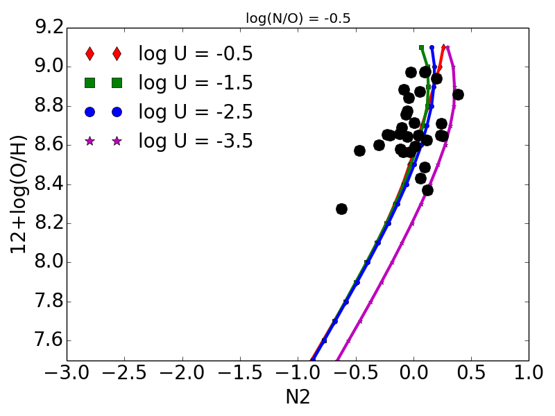
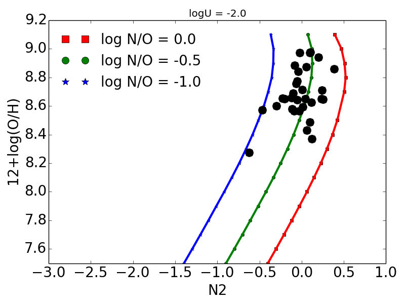
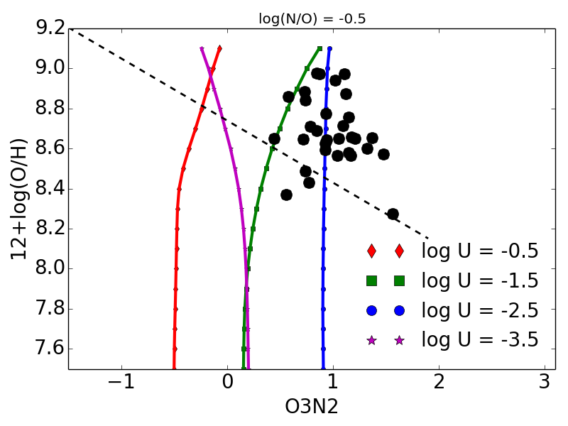
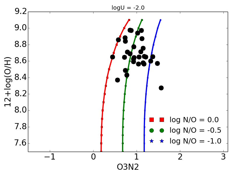
Figure 4: Relation between the total oxygen abundance 12+log(O/H) with the emission line ratio N2 (upper panels) and O3N2 (lower panels) both for the abundances derived by Dors et al. (2017) for the control sample and from some of the models described in the text at a fixed log(N/O) = -0.5 (left panels) and at a fixed log($U$ )= -2.0 (right panels). The dashed black lines represent the empirical calibrations for star-forming regions derived by Pérez-Montero & Contini (2009).

In Figure 4 we see the relation between O/H and N2 both for the abundances derived by Dors et al. (2017) for the control sample and for the predictions made by some of the models of our grid for different values of $U$ and N/O. The relation is monotonically growing up to very high values of metallicty but it presents a large dependence on N/O, as in the case of star-forming regions as pointed out by Pérez-Montero & Contini (2009). The dependence on $U$ is slightly lower but can also be important. We also see that the empirical calibration given for star-forming regions cannot be used for this kind of objects, as it underestimates the derived metallicity.

Other observable based on [N ii] emission lines that we can use to constrain both O/H and $U$ is O3N2, defined by Alloin et al. (1979) as:

$${\rm O3N2}=\log\left(\frac{[{\rm O\textsc{iii}}]\lambda 5007}{H\beta}\cdot\frac{H\alpha}{[{\rm N\textsc{ii}}]\lambda 6583}\right)$$ (11)

The relation of this parameter with total metallicity is also shown in Figure 4 both for the studied sample of galaxies and for models attending to their dependence on N/O and $U$. As can be seen it strongly depends on both parameters given the large correlation of the [O iii]/H$\beta$ ratio with excitation (Storchi-Bergmann et al., 1998). On the other hand, the relation of this parameter with O/H is totally different to the behavior observed in star-forming regions where, for the high-metallicity regime, the parameter decreases for larger values of O/H and remains relatively unaffected for low values of $Z$, so the linear relation is not usually defined for high values of O3N2 (i.e. O3N2 $>$ 2). In contrast, for NLRs of AGNs this parameter grows with O/H above all for large metallicity and high $U$ because the relative abundance of the ions emitting in the optical part of the spectrum begins to be important and play a more relevant role in the cooling of the gas at this regime.

In addition, among the observables used by the code to derive O/H and log($U$ are the R23 parameter, defined by Pagel et al. (1979) as:

$${\rm R23}=\frac{[{\rm O\textsc{ii}}]\lambda 3727+[{\rm O\textsc{iii}}]\lambda\lambda 4959+5007}{H\beta}$$ (12)

Note that this parameter is traditionally defined using the other strong [O iii] line at $\lambda$4959 Å, so in the case of our code, which uses the theoretical ratio of this line with $\lambda$5007 Å (i.e. I(5007)/I(4959) = 3), this does not imply any difference if the ratio is calculated in the same way for the observable. The relation between log R23 for the sample of objects and the models are shown in Figure 5. This parameter presents a totally different behavior for high values of $U$ to that observed in star-forming regions as it is not double-valued (i.e. R23 increases for low O/H and decreases for high O/H). On the contrary, it presents a monotonically growing relation with O/H up to very high values. As previously explained for other observables based on [O iii] lines this is mostly due to the fact that, according to our models, most of oxygen keeps in higher ionization stages than those whose emission-lines can be measured in the optical part of the spectrum. As a consequence, these lines act as effective coolants of the gas in AGNs at a much higher metallicity than in the case of star-forming regions. In addition it is observed, as in the case of star-forming regions (e.g. Pérez-Montero & Díaz 2005) that this ratio has a strong dependence on $U$, what can even affect the shape and the turnover of this relation.

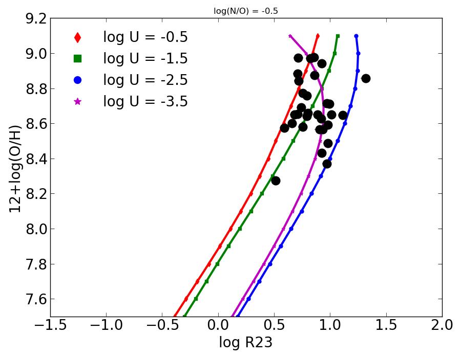
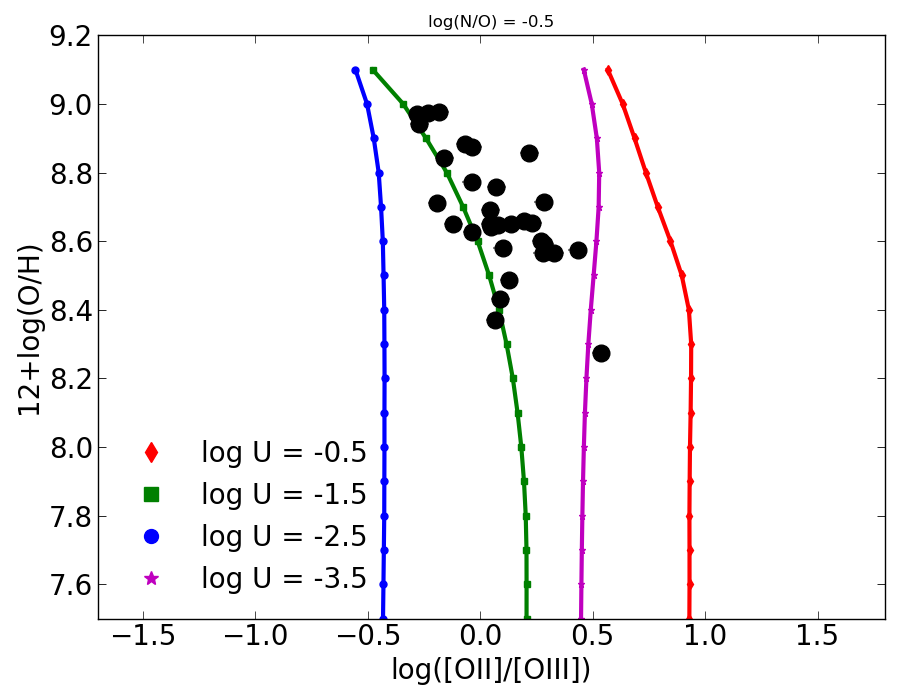
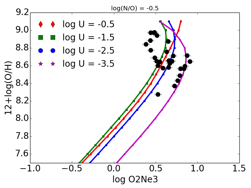
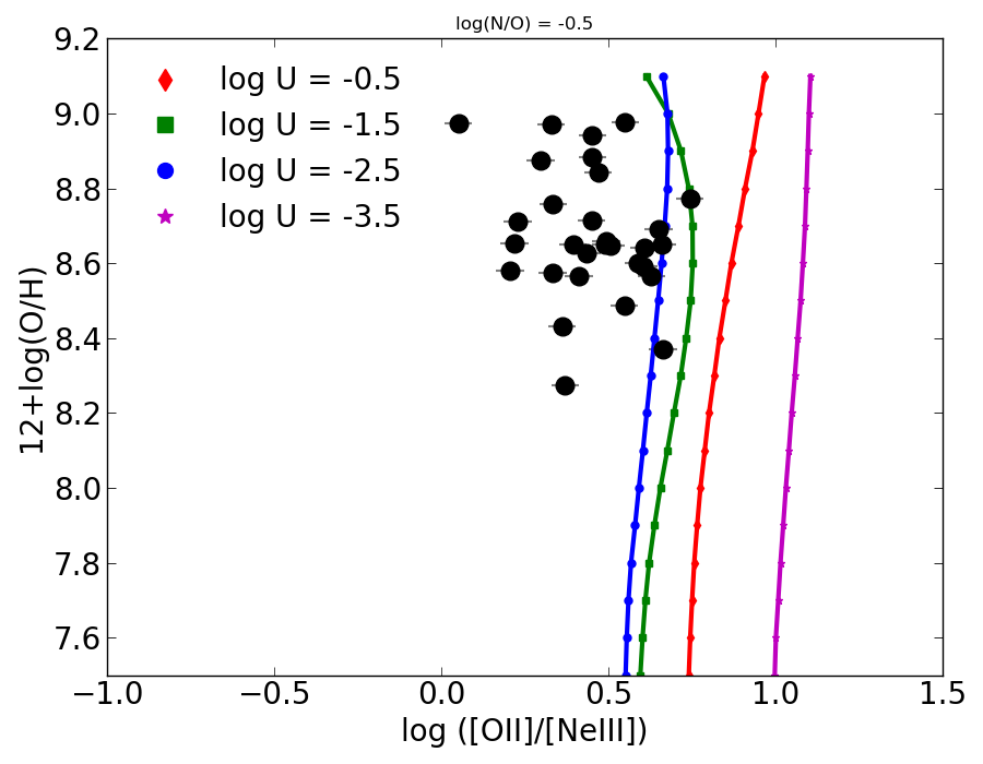
Figure 5: Relation between the total oxygen abundance 12+log(O/H) as derived in Dors et al (2017) for the control sample with the emission line ratios R23 (left upper panel), [O ii]/[O iii] (right upper panel), O2Ne3 (left lower panel), and [O ii]/[Ne iii] (right lower panel). All panels also show results from some of the models described in the text at a fixed log(N/O) = -0.5. .

To minimize this dependence, the code also considers the ratio [O ii] $\lambda$3727/[O iii] $\lambda$$\lambda$4959+5007, what helps to restrict the values of the ionization parameter. This is also shown in Figure 5, where we can see that this ratio presents a dependence on metallicity much lower than in the case of R23.

Nevertheless the dependence of this emission-line ratio on $U$ is not monotonic as can be seen in Figure 6 as predicted from models. The ratio decreases as $U$ increases, as it is expected and it occurs in star-forming regions, but, for values of log($U$) larger than -2.0, it begins to turn and it increases giving place to a double-valued relation. This bivaluated behavior is also seen for other observables based on [O iii] lines, as it is the case for O3N2 and can also be seen in the same Figure. This simply happens because at high values of $U$ the relative intensity of [O iii] decreases rapidly as oxygen is ionized on higher stages. Therefore to overcome the problem of a degeneration in the derivation of $U$ using this emission-line ratio we do not consider in our models all values with log($U$) lower than -2.5, that is the value for which O3N2 reaches it maximum. The range of log $U$ considered in our models cover the typical values in other works studying similar objects (e.g. Dopita et al. 2014), and does not affect the determination of N/O and O/H as shown in the next section.

Finally, the code also allows to use the [Ne iii] $\lambda$3868 Å emission line, but it is only used as a alternative to [O iii] $\lambda$5007 Å when this is not given (i.e. for specific setups where [O iii] is not covered), as these two ions present a quite similar ionization structure and the [Ne iii] line can be used as a proxy for the intensity in the high-excitation region at very blue wavelengths, as discussed in Pérez-Montero et al. (2007). In this way, the O2Ne3 can be defined as:

$${\rm O2Ne3}=\frac{[{\rm O\textsc{ii}}]\lambda 3727+[{\rm Ne\textsc{iii}}]\lambda 3868}{H\beta}$$ (13)

Note that in this definition, contrary to Pérez-Montero et al. (2007), no empirical factor has been considered for the intensity of [Ne iii], as this is not required by the code to compare the observed fluxes with the results from models. The relation between the O2Ne3 parameter with O/H, and the same relation with the [O ii]/[Ne iii] as an indicator of the excitation are also shown in the lower panels of Figure 5. As can be seen both observables behave in very similar way to those based on [O iii] and therefore can be used instead by the code to derive abundances and excitation in NLRs of AGNs.

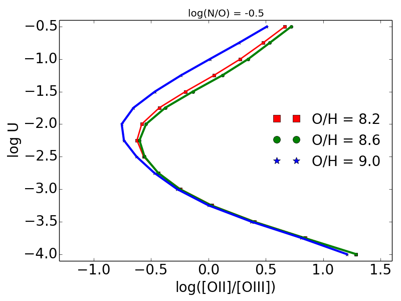
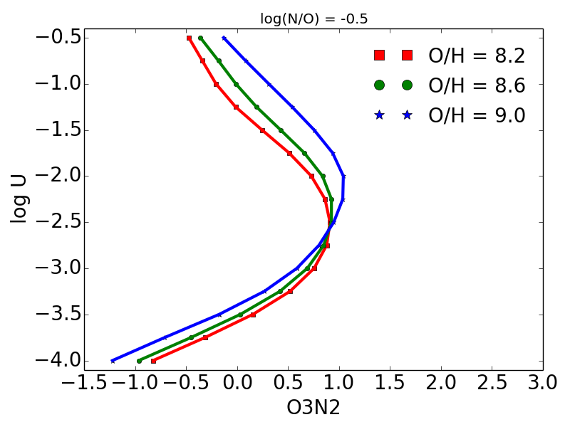
Figure 6: Relation between the ionization parameter and the emission-line ratios [O ii]/[O iii] (at left), and O3N2 (at right) as predicted from photoionization models for different metallicities and assuming a constant N/O value at -1.0.

4 Results and discussion

4.1 Resulting properties of the sample

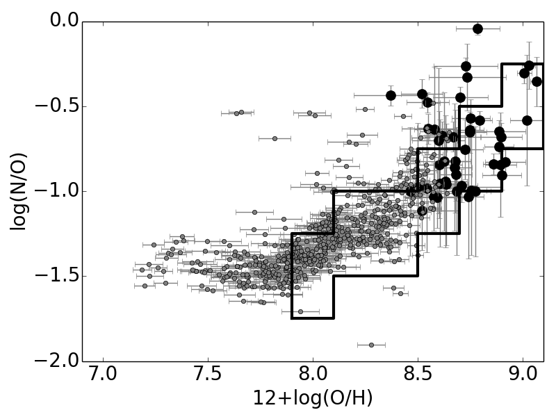
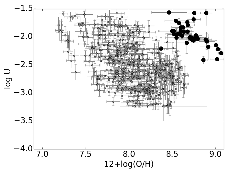
Figure 7: Relations between O/H and N/O (left) and $U$ (right) for the resulting values of our method for the control sample. Grey points represent the sample of star-forming regions analyzed following a similar bayesian-like procedure by Pérez-Montero (2014). The solid black line encompasses the space of models empirically constrained by Pérez-Montero (2014) used to derive O/H when no previous derivation of N/O is performed.

In this subsection we discuss the results obtained by using the HCm code for the 47 Seyfert 2 and 1.9 galaxies presented in Dors et al. (2017)) when all the available emission-lines required by our code are used. The results of the code include too associated uncertainties which are quadratical additions of those from the standard deviation ot the $\chi^{2}$-weighted distribution of the input grid values and the dispersion from the distribution of results after 100 Monte-Carlo iterations using the input reddening-corrected lines randomly perturbed with their errors.

In left panel of Figure 7 we show the resulting O/H and N/O abundance ratios and their corresponding errors. The ranges of metallicity are quite similar to those obtained using the tailor-made models presented in Dors et al. (2017), going from 12+log(O/H) = 8.37 to 9.07 (from 0.5 to 2.4 times the solar metallicity, taking as reference the value 12+log(O/H)_⊙ = 8.69 in Asplund et al. 2009). Regarding nitrogen, the range in log(N/O) goes from -1.11 to -0.04 (equivalent to the range 0.6 to 6.6 times the solar N/O ratio) (taking as log(N/O)_⊙ = -0.82 from Asplund et al. 2009). These values are in concordance with the expected relation between O/H and N/O in a regime of secondary nitrogen production, giving place to an enhancing N/O ratio for higher metallicities (e.g. Henry et al. 2000), although with a large dispersion. In the same Figure we compare the obtained abundances with those derived using HCm for star-forming objects Pérez-Montero (2014) for the sample presented by Marino et al. (2013). As can be seen the type 2 AGNs occupy the regions of high-metallicity star-forming regions in agreement with the results obtained by Dors et al. (2017), but a non-negligible fraction of the analyzed objects lie in a region outside the expected relation what justifies the use of a previous determination of N/O to derive O/H abundances using [N ii] emission lines, instead of assuming any expected relation between O/H and N/O.

Regarding the relation between metallicity and ionization parameter, in right panel of Figure 7 we show the values obtained by our code for the same sample. In this case, the range of log$U$ looks to be much more constrained (log$U$ goes from -2.42 to -1.27). In contrast to the relation between abundance ratios, there is not any similarity with the behavior observed for star-forming regions as can be seen in the same plot. On one hand the average $U$ is much higher in the case of AGNs than for the star-forming regions, even taking into account that the average metallicity of these is much lower. This behavior is also observed even if the grid of models is not constrained to the higher values of $U$. The existence of a possible relation between O/H and $U$ as for star-forming objects, in the sense that galaxies with higher metal content are in average less excited, is very uncertain and must be more deepley studied. In any case, unlike star-forming objects, the code does not require any restriction in the space of models between O/H and $U$ when no [O iii] 4363 Åis introducied as input, as it will be discussed below.

4.2 Comparison with the control abundances

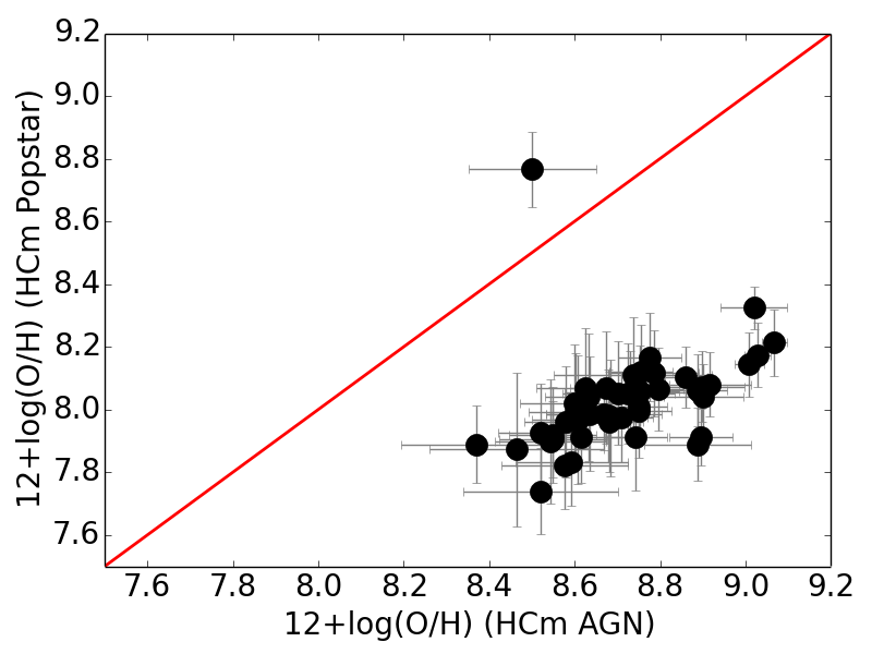
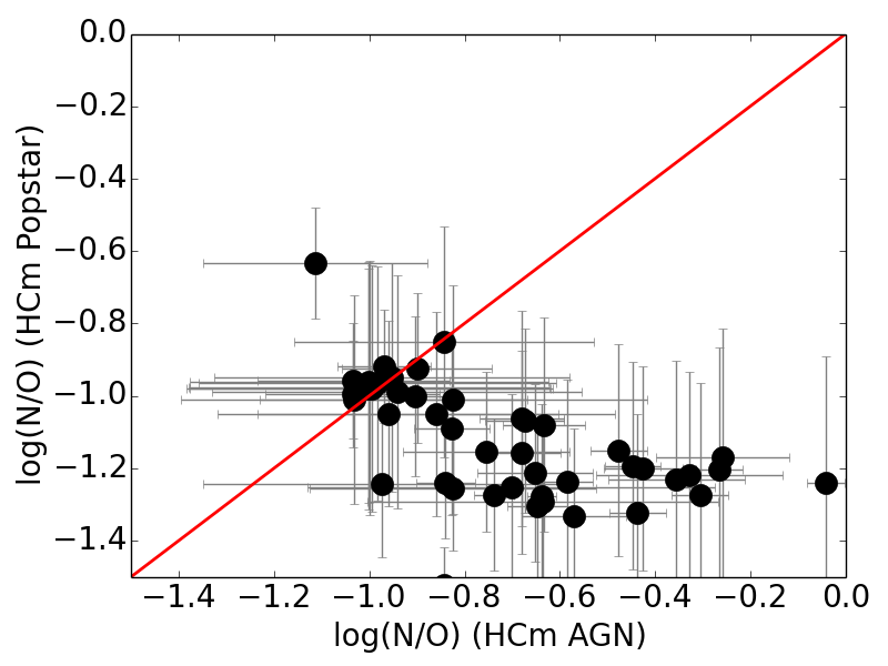
Figure 8: Comparison between chemical abundances derived using the method described in this work and those obtained assuming the ionizing spectral energy distribution of a massive young star cluster for the control sample. At left comparison of derived 12+log(O/H) and at right for log(N/O). The red solid line represents the 1:1 relation.

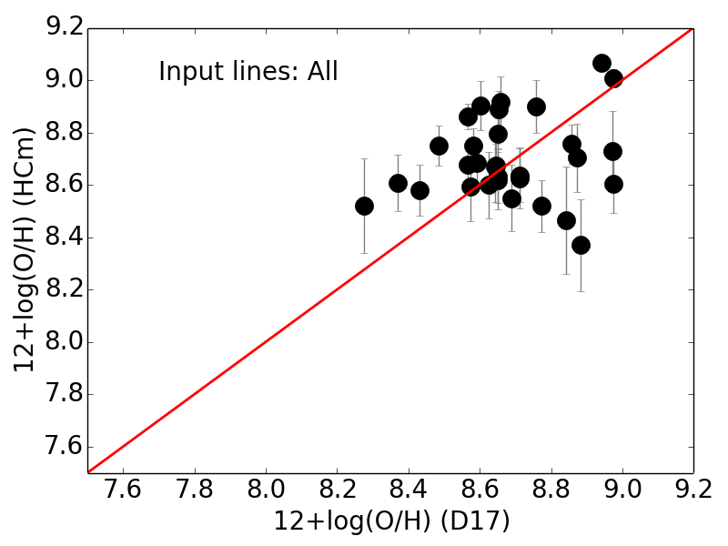
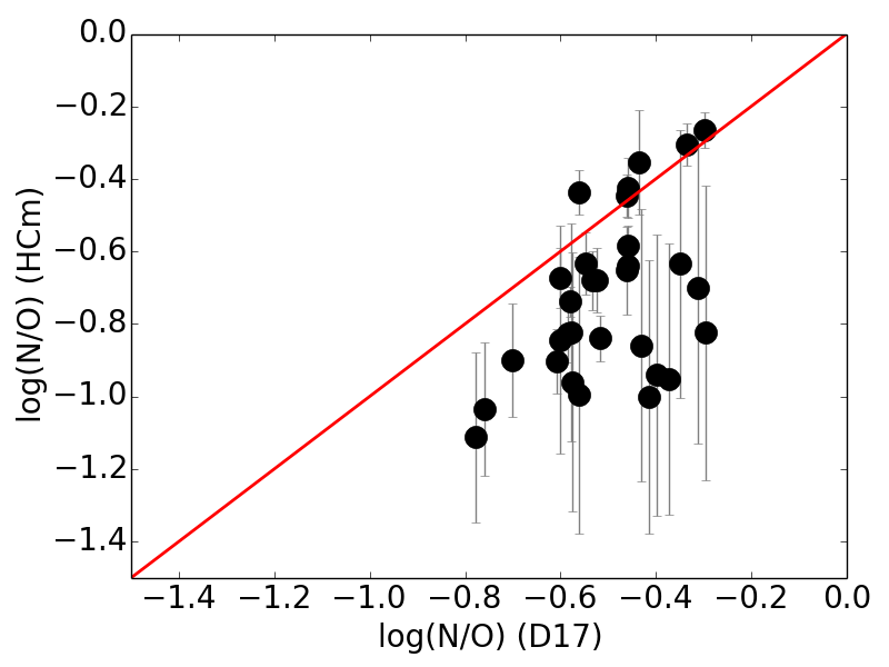
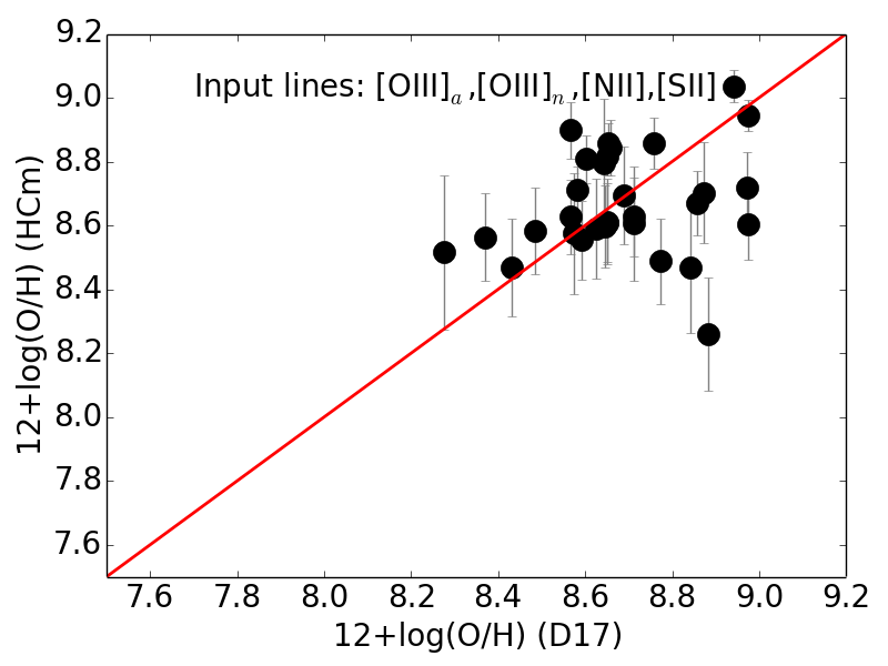
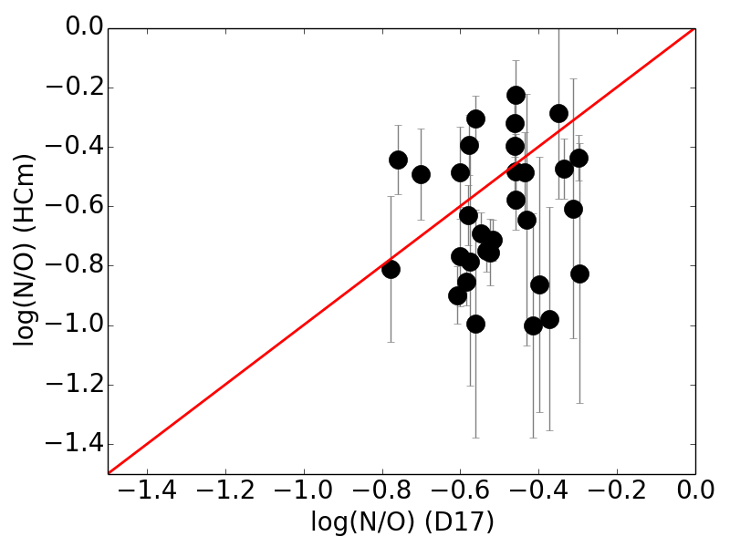
Figure 9: Comparison between chemical abundances derived using the method described in this work and those taken from Dors et al. (2017) from tailored photoionization models. At left comparison of derived 12+log(O/H) and at right for log(N/O). The upper panels show the comparison when all the lines are used while lower panels show the comparison in absence of [O ii] $\lambda$3727 Å. The red solid line represents the 1:1 relation.

In this subsection we discuss the deviations in the resulting chemical abundances obtained from HCm code using different sets of emission-lines taking as reference the abundances of the control sample obtained by a Dors et al. (2017) using detailed tailor-made models.

The first comparison that we can perform as a test is to check to what extent the use of a specific SED for our models impact on the determination of the final chemical abundances. To this aim we introduced the compiled emission lines in the analyzed sample of Sy2 galaxies using the same code HCm, but making use of a SED of massive young star clusters taken from popstar (Mollá et al., 2009) with the features described in Pérez-Montero (2014). This comparison is shown both for O/H and N/O in Figure 8. As can be seen the obtained abundances when we assume a massive cluster SED is much lower both for O/H (0.7 dex in average) and N/O (0.4 dex in average) than the abundances derived from the same code assuming the appropriate power-law SED. This comparison illustrates the importance of the input SED in the final results.

Continuing with our analysis of the results, In Figure 9 we show the total oxygen abundances and the nitrogen-to-oxygen ratio obtained from our code using as input the appropriate AGN SED as compared with the values derived by Dors et al. (2017) and introducing all possible emission lines. In this way there is now a good agreement between the two sets with average deviations lower in most cases than the average uncertainty and with dispersions of the same order, although it is noticeably worse for N/O. Both the mean and the standard deviation of the residuals for the analyzed Sy2 galaxies are listed in Table LABEL:dispersion. From this table it is easy to establish a comparison between the results from our code using all emission lines and only different subsets.

In the lower panels of the same Figure we show the comparisons when the emission-line of [O ii] at $\lambda$3727 Å is not included as input in the HCm code. This is usual in some setups when the very blue part of the spectrum is not available (e.g. in the Sloan Digital Sky Survey at very low redshifts). As can be seen the agreement in this case is good, with deviations from the abundances in the control sample lower in all cases than the usual obtained uncertainties.

Table 1: Mean and standard deviation of the residuals of the comparison between the resulting O/H and N/O abundance ratios derived for HCm using all involved lines and using only a constrained set of them as compared with the values for the same objects obtained in Dors et al (2017). In the table [O ii] stands for $\lambda$3727 Å, [Ne iii] for $\lambda$3868 Å, [O iii]_a for $\lambda$4363 Å, [O iii]_n for $\lambda$5007 Å, [N ii] for $\lambda$6583 Å, and [S ii] for $\lambda$$\lambda$6717+6731 ÅÅ.

	Set of input emission lines	Mean $\Delta$(O/H)	St.dev. $\Delta$(O/H)	Mean $\Delta$(N/O)	St.dev. $\Delta$(N/O)
	All lines	- 0.01	0.21	+ 0.23	0.19
	[O iii]a, [O iii]n, [N ii], [S ii]	+ 0.02	0.21	+ 0.12	0.24
	[O ii], [O iii]n, [N ii], [S ii]	- 0.08	0.32	+ 0.08	0.12
	[O iii]n, [N ii], [S ii]	+0.15	0.26	- 0.11	0.11
	[N ii], [S ii]	+ 0.29	0.29	- 0.12	0.10
	[O iii]n, [N ii]	-0.24	0.15	- –	–
	[N ii]	- 0.25	0.16	- –	–
	[O ii], [O iii]n	- 0.11	0.21	–	–
	[O ii], [Ne iii]	- 0.13	0.30	–	–

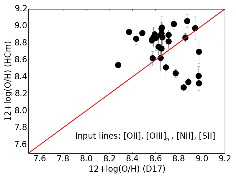
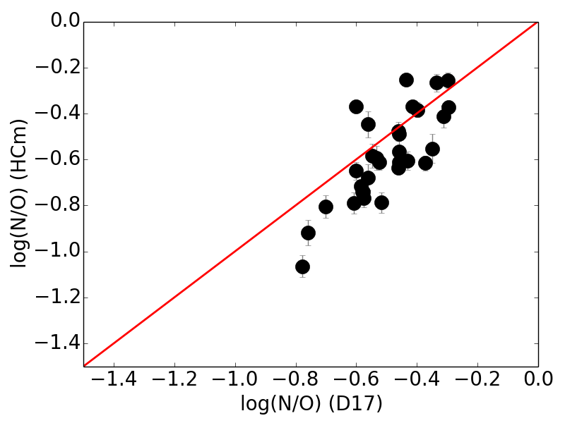
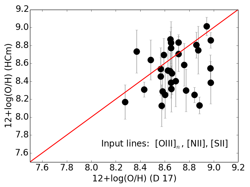
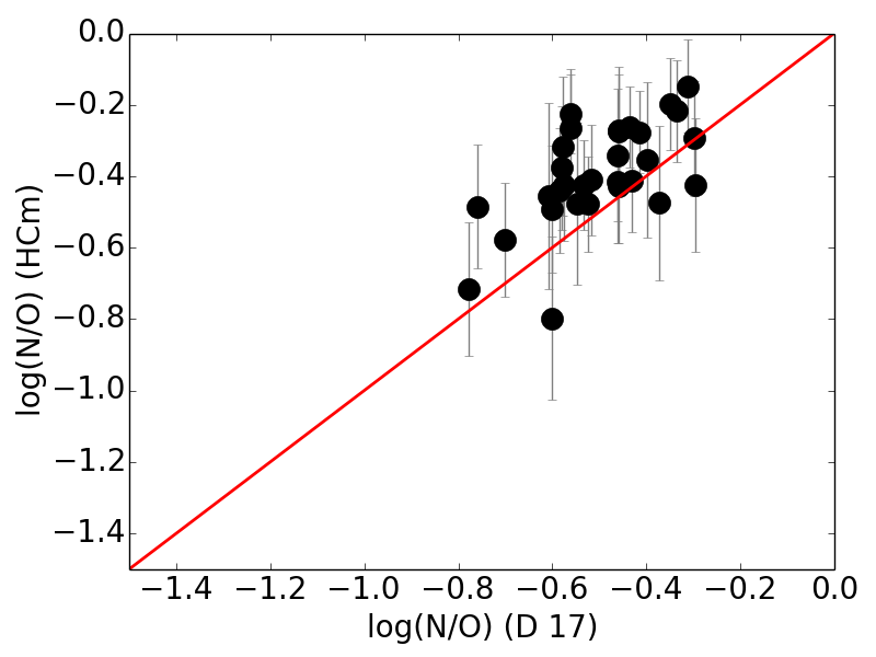
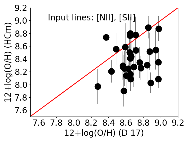
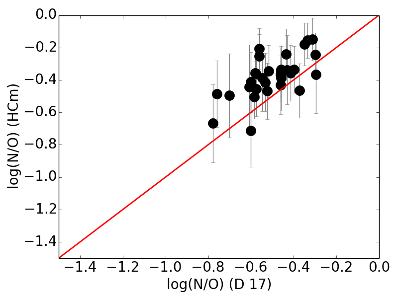
Figure 10: Comparison between the chemical abundances derived from our method when only certain sets of lines are considered and the abundances derived in Dors et al (2017) for the control sample. In top row, in absence of [O ii] $\lambda$3727 Å; in middle row when [O ii] and [O iii] $\lambda$4363 Å are not included and, in bottom row, when only [N ii] 6573 Å and [S ii] $\lambda$$\lambda$6717,31 ÅÅ are included. At left comparison of derived 12+log(O/H) and at right for log(N/O). The red solid line represents the 1:1 relation.

When the [O iii] $\lambda$5007/4363 Å temperature-sensitive emission-line ratio cannot be measured in star-forming regions (or any other of the auroral-to-nebular line-ratios corresponding to other ionic species can be measured instead) implies that the so-called $T_{e}$ method (i.e. the calculation of all chemical ionic abundances from a measured estimation of the electron temperature) cannot be used and other methods based only on strong emission-lines can be adopted instead. In the case of the HCm code for star-forming regions, as described in Pérez-Montero (2014), this implies the adoption of an empirical relation between metallicity and ionization parameter. In the case of AGNs, though this dependence between $Z$ and $U$ is also found,, in absence of the [O iii] $\lambda$4363 Å lines there is no need to assume any extra relation to get accurate abundances with the rest of strong lines, as there are not degeneracies between metallicity and the used optical emission-line ratios in the remaining grid of models for log $U$ $>$ -2.5.

In Figure 10 we show both O/H and N/O derived by our code for the sample of analyzed galaxies when we just get a limited number of optical emission lines as compared with the abundances derived by Dors et al. (2017). Using as input not all required lines can be caused by a limited sensitivity or spectral coverage of our detector. The mean offsets and standard deviation of the residuals are listed in Table LABEL:dispersion.

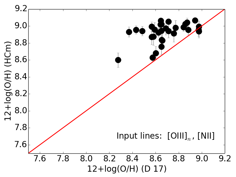
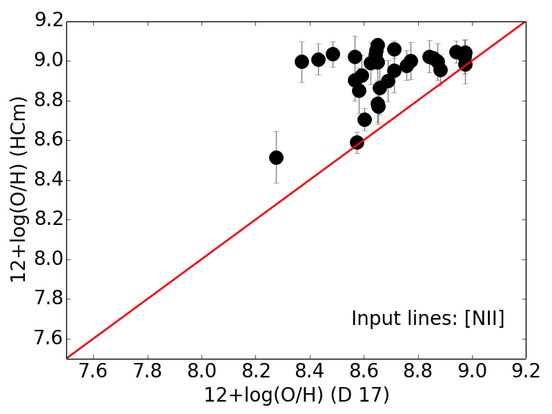
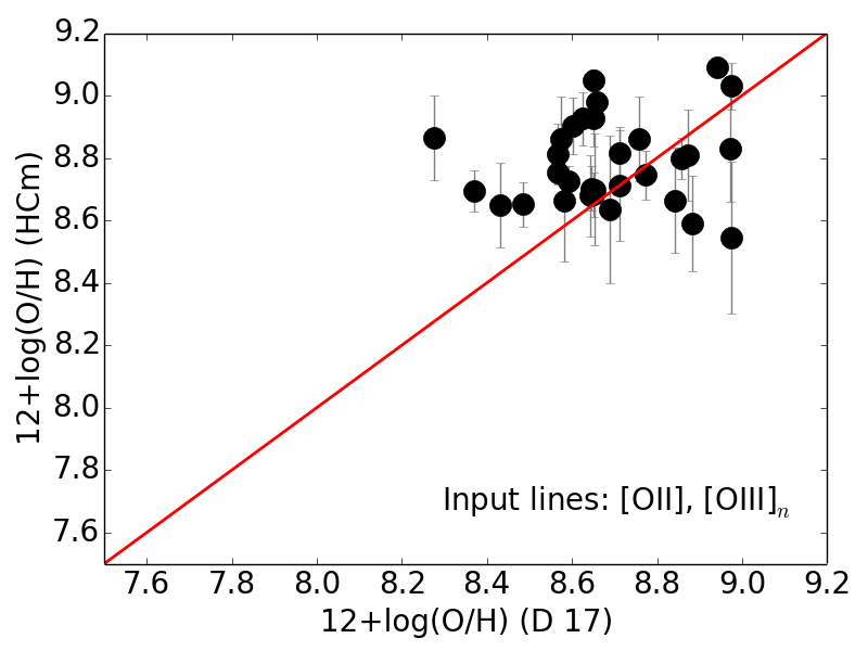
Figure 11: Comparison between the oxygen abundances derived from our method when only certain lines are considered as input and a previous derivation of N/O is not carried out but an empirical O/H-N/O relation is adopted with respect to the values presented by Dors et al (2017) for the control sample. In the upper left panel using O3N2, in the right upper panel, using N2, in the lower left, using only [O ii] $\lambda$3727 Å and [O iii] $\lambda$5007 Å, and, at lower right, using [O ii] and [Ne iii] $\lambda$3868 Å. The red solid line represents the 1:1 relation.

In the case that no [N ii] $\lambda$6583 Å emission line is detected in combination with another low-excitation line emitted by an $\alpha$ element, such as [O ii] or [S ii], the code cannot calculate N/O. In this case the code assumes the relation between O/H and N/O to follow the expected relation derived from most star-forming regions and which can be seen in the Figure 7. For lower values of metallicity N/O remains constant and low due to that most of N production has a primary origin. As O/H enhances, at a value 12+log(O/H) $\sim$ 8.0, N/O begins to grow with metallicity as N has mostly a secondary origin. We assume for our models this restriction in case N/O cannot be estimated, but this can produce deviations in those objects where this behavior is not followed due to strong interactions with the intergalactic medium (e.g. Köppen & Hensler 2005). In all case, this assumption is behind most of the usual empirical and model-based calibrations based on [N ii] lines even if this relation has not been very well studied in the case of AGNs that can deviate from the behavior observed in star-forming regions, so it is strongly preferable to have a good previous estimation of N/O.

In Figure 11 we show the comparison between the O/H values derived by our code and those calculated by Dors et al. (2017) when no previous N/O is derived and a law between O/H and N/O is assumed instead, for the case that we use as input lines O3N2 and N2. The mean offsets and the standard deviations of the residuals are shown in Table LABEL:dispersion.

In case that no N/O previous calculation can be carried out, the code can also provides us with a solution for O/H and $U$ using only [O ii] and [O iii] lines, or alternatively, in case the observed wavelength range is limited and only very blue lines are observed, using only [O ii] and [Ne iii] as input of the code, as discussed in hte previous sections The comparisons between the total oxygen abundances obtained for these cases and those from the control sample are shown in the lower panels of Figure 11. The corresponding means and deviations are also listed in Table LABEL:dispersion.

4.3 Changing the resolution and range of the input grid

According to Pérez-Montero et al. (2016) the use of a discrete grid of input values in HCm can lead to a somehow discrete distribution of the results that is above all noticeable for large samples of objects. For this reason in the case of star-forming objects, HCm also supplies interpolations in the grid that multiplies in a factor 5 the resolution in the three main input drivers of the grid (i.e. O/H, N/O, and $U$). In this version for NLRs of AGNs, this is also possible. In Figure 12 we show the comparison between the results for O/H and N/O for the control sample when using the code with a interpolated and a non-interpolated grid of models. As can be seen in both cases the agreement is very good and no deviations beyond the obtained errors are produced (i.e. the standard deviation of the residuals is in both cases lower than 0.02 dex).

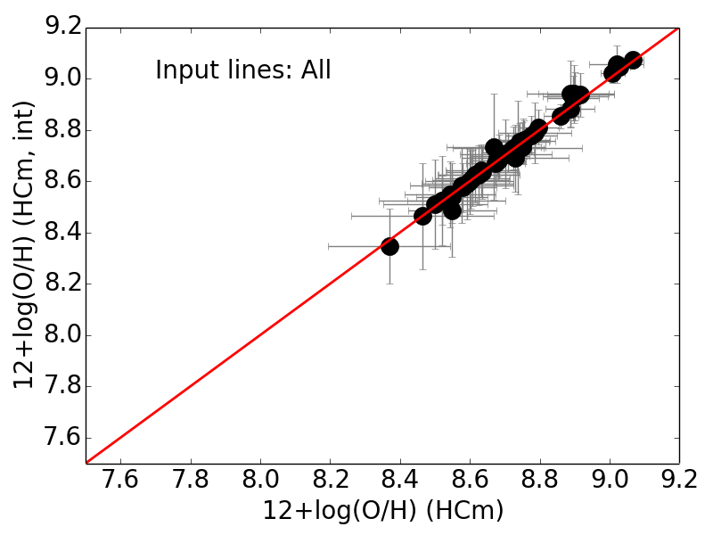
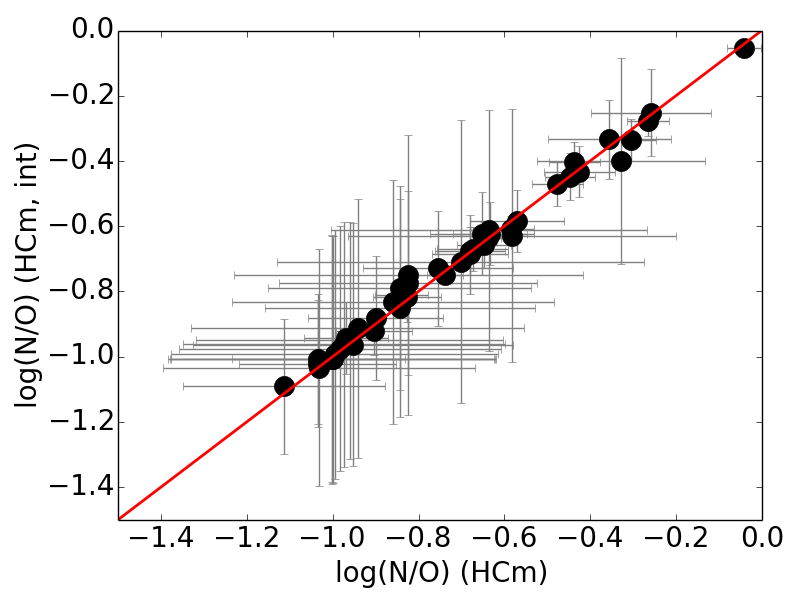
Figure 12: Comparison between the resulting O/H (left panel) and N/O (right panel) derived by HCm using a non-interpolated and an interpolated grid of models. In both panels the red solid line represents the 1:1 relation.

Regarding the range of chosen input parameters in the models, abundances were selected to cover the expected values observed in many NLRs and the extrapolation to the central regions in spiral galaxies. The fact that the code recovers the values found in Dors et al. (2017), who do not consider any abundance restriction on their detailed search, probes that at least in this sample this range is appropriate. In the case of the chosen restriction for log $U$ (i.e. only values log $U$ $>$ -2.5) we explore to what extent this can affect the final derived abundances. In Figure 13 we show the comparisons between the abundances and $U$ obtained by the code when all values in the grid are taken and when only the restricted range of $U$ is assumed. As it can be seen in the case of O/H and N/O this restriction does not imply any difference within the errors. On the other hand the average log $U$ is 0.18 dex larger in average when the low values of $U$ are not taken, as can be expected as in the weighted means no models with very low values of $U$ are considered. Nevertheless, as can be seen also in the lower right panel of the same Figure, a large fraction of the objects whose $U$ was calculated using the entire range of $U$ lie in a region without any model that corresponds to the turnover region of the relation between [O ii]/[O iii] versus $U$. Although the choice of the upper branch in this relation can look arbitrary this is the range expected for most AGNs (e.g. Dopita et al. 2014).

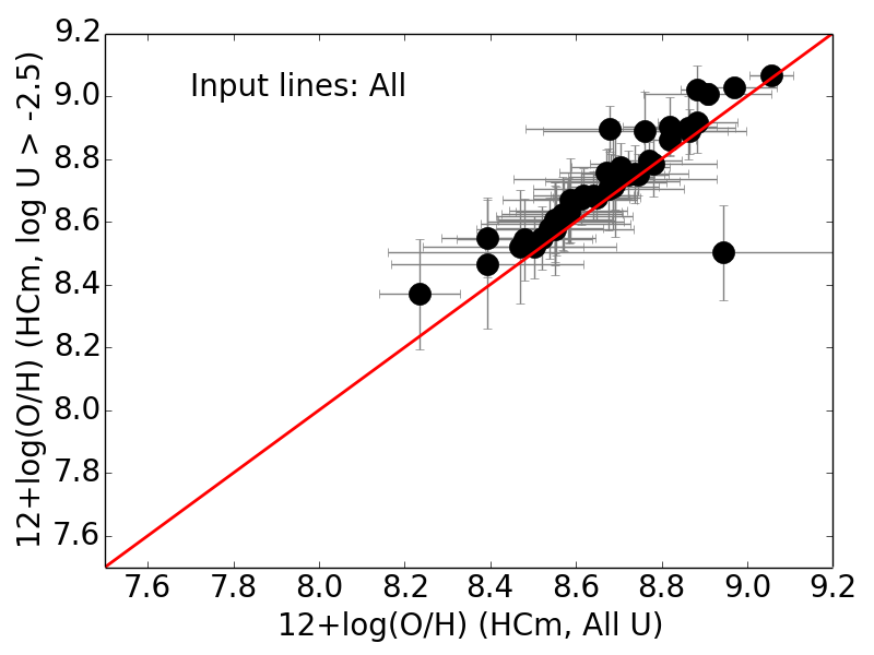
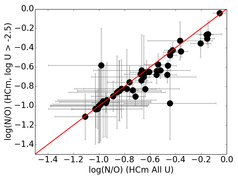
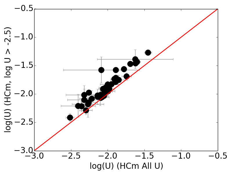
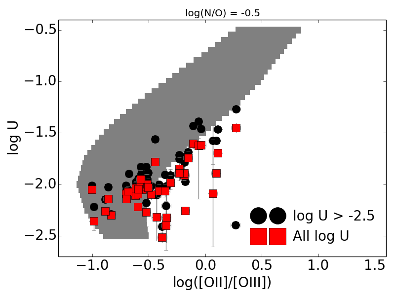
Figure 13: Comparison between the resulting O/H ( upper left panel), N/O (upper right panel), and log $U$ (left lower panel) derived by HCm using a non-restricted and a $U$-restricted grid of models. In all these panels the red solid line represents the 1:1 relation. The right lower panel represents log $U$ as a function of the [O ii]/[O iii] emission-line ratio with models with O/H $\geq$ 8.4 as grey squares, black circles as results for the control sample in a $U$-restricted grid, and red squares as results for a non-restricted grid.

4.4 Consistency of models with the $T_{e}$ method

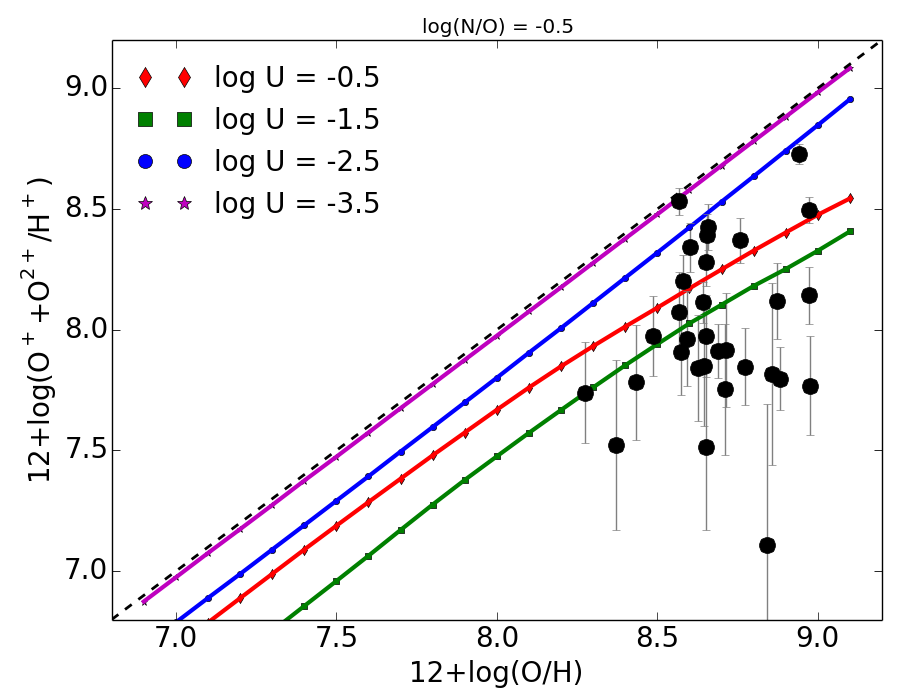
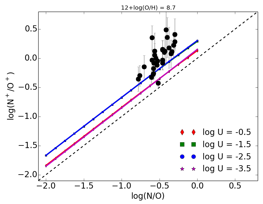
Figure 14: Comparison between total oxygen abundance and the addition of the abundances of the two main ions observed in the optical part of the spectrum (i.e. O⁺ and O²⁺), at left, and between N/O and the corresponding ion abundance ratio N⁺/O⁺, at right. Models are represented using solid lines for different values of $U$. In both panels the black circles represent the data from Dors et al (2017) whose total abundances where calculated using tailored models, while their ionic abundances were calculated following the $T_{e}$ method. The dashed black line represents the 1:1 relation.

It is known that the application of the $T_{e}$ method to derive total chemical abundances in the NLRs of type-2 AGNs can lead to very low values as compared to those from photoionization models (e.g. Dors et al. 2015). This discrepancy can be interpreted in terms of the usual offset that can be found between results from the $T_{e}$ method and models, or to a different physics governing the ionization of the plasma. Since the code HCm does not lead to any difference between its predictions and the application of the $T_{e}$ method in star-forming regions (Pérez-Montero, 2014), we can evaluate possible explanations to this discrepancy using the version of the code for AGNs.

In Figure 14 we show the comparison between the total oxygen abundance derived by Dors et al. (2017) for the compiled sample of Sy2 galaxies, compared to the O⁺ + O²⁺ relative to H⁺ ionic abundances derived following the $T_{e}$ method as described in Pérez-Montero (2017). This is based on a previous determination of the electron temperature from the emission-line ratio [O iii] $\lambda$$\lambda$5007/4363 ÅÅ. As can be seen, the objects lie in a range below the 1:1 relation as the addition of the relative abundance of O⁺ and $O^{2+}$ is much lower than the total abundances derived from models, that is 0.7 dex in average.

We plot in the same figure the predictions made by the grid of models described in previous sections and we can see that this difference is naturally explained by the models in terms of a large fraction of oxygen that it does not appear as the ions whose abundances can be derived using the optical emission-lines. According to models, the difference between the total oxygen abundance and the optical ionic fractions depends strongly on total metallicity and ionization parameter and can reach up to 0.8 dex.

This difference underlines the importance of using models to derive the total abundance of oxygen in the NLRs of AGNs using optical lines as the ionization correction factor (ICF) for O⁺+O²⁺, contrary to star-forming regions, is far to be negligible.

In the right panel of the same Figure we represent a similar relation comparing the total N/O ratio with the corresponding ionic fraction N⁺/O⁺. In this case this ionic fraction cannot be neither used as a proxy of N/O, as the empirical ionic ratio is in average 0.5 dex larger than the total elemental ratio. This offset is due to that the ionization structure of oxygen and nitrogen present more differences than in the case of nebulae ionized by massive stars, and N⁺ represents a much larger fraction of N than O⁺ of oxygen. In consequence, as in the previous case, models are necessary to provide accurate ICFs to derive total chemical abundances from the observed ionic fractions using optical emission lines.

4.5 Dependence on other input conditions

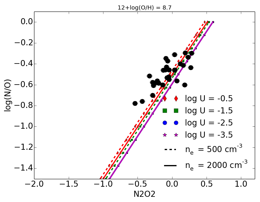
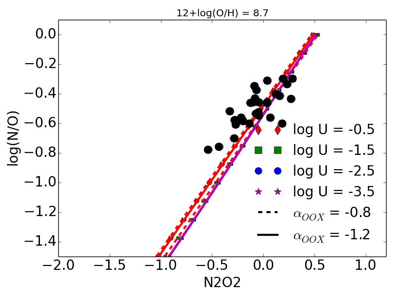
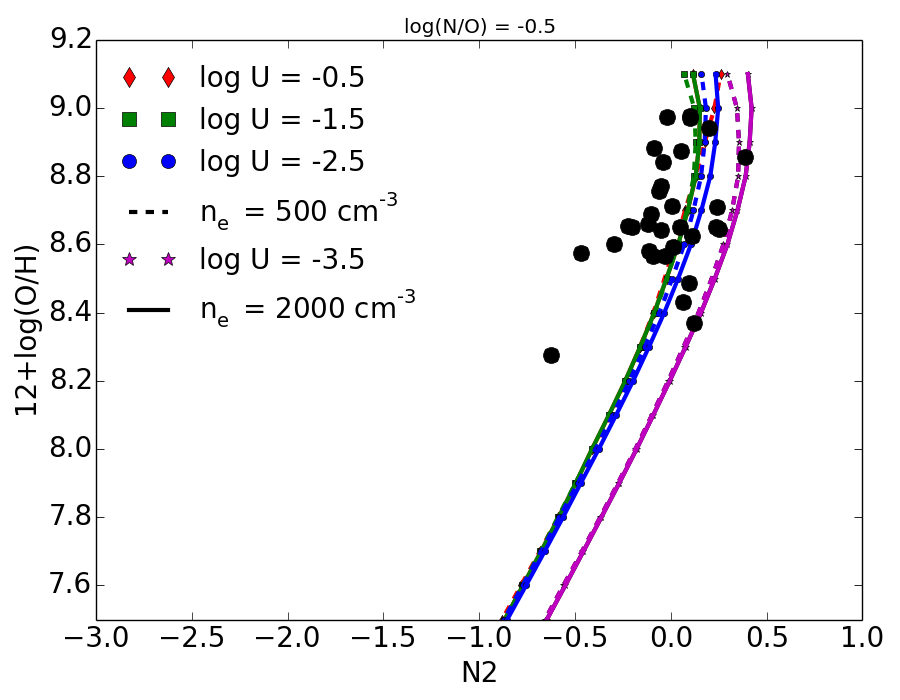
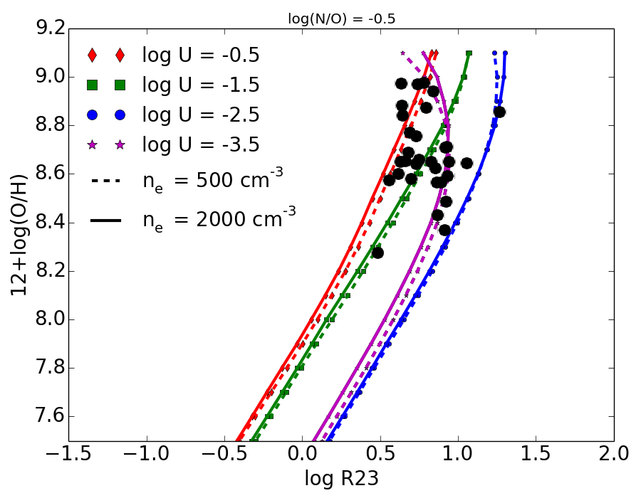
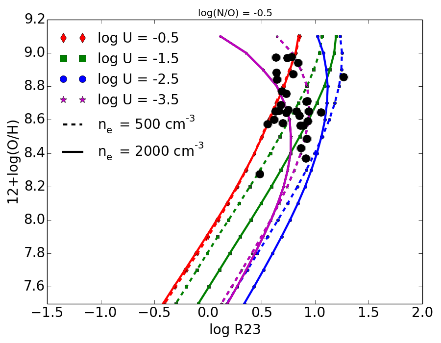
Figure 15: Relations between different emission-line observables and abundances ratios used in the models as a function of different input parameters. Panels in the left column show the difference between models using an electron density of 2000 cm^-3 (solid line) and 500 cm^-3 (dashed line). The panels in the right column shows the difference between and $\alpha_{OX}$ for the input ionizing SED of -1.2 (solid line) and -0.8 (dashed line). In the upper panels we show the relation between N2O2 and N/O for some models at a fixed 12+log(O/H) = 8.7, in the middle panels the relation between N2 and O/H for some models at a fixed log(N/O) = -0.5 and in the bottom panels between R23 and O/H for some models at a fixed log(N/O) = -0.5.

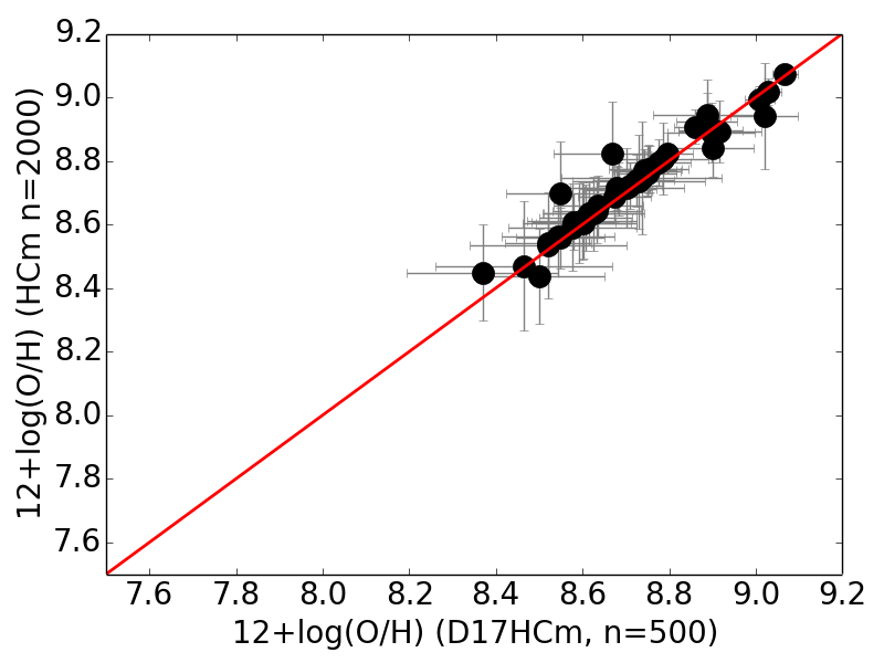
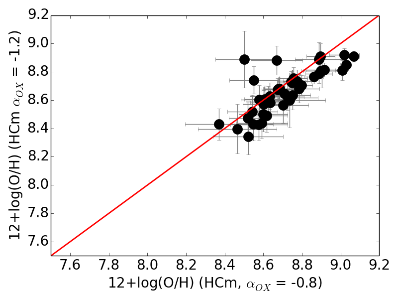
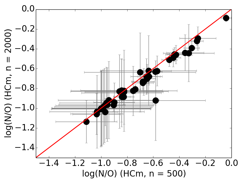
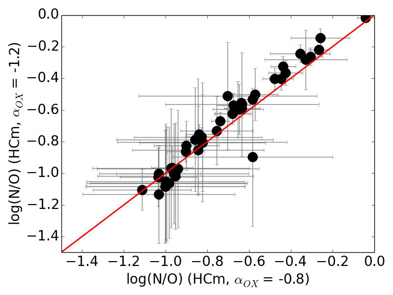
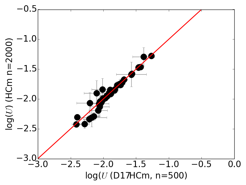
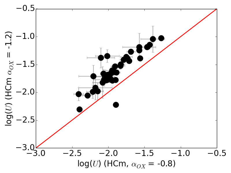
Figure 16: Comparison between O/H (upper row), N/O (middle row) and log $U$ )lower row) from our method and all input emission lines using the grid of models with an electron density of 500 cm^-3 and a $\alpha_{OX}$ = -0.8 and the results from the same code but changing two parameters in the input grid of models. In left column changing density to n_e = 2000 cm^-3 and in the right column changing $\alpha_{OX}$ to -1.2. The red solid line represents the 1:1 relation.

In this subsection we discuss how varying other input factors in the models can impact the absolute values and uncertainties of the final derived abundances in our method. Although there are multiple possible sources of uncertainty in the adopted input values in the models that can affect our results in this paper we focus on electron density and the $\alpha_{ox}$ parameter as these are among those more difficult to be accurately estimated in NLRs of AGNs (e.g. Dors et al. 2019).

Electron density is one of the physical properties of the gas that can affect the emissivity of the observed emission lines. Although it is known that below the critical density the collisional de-excitation is negligible in this case, it is important to quantify to what extent this can affect the final derived abundances. In Figure 16 we show the comparison between the obtained O/H, N/O, and log $U$ values derived by HCm . When we changed the input electron density from 500 to 2 000 particles per cm^-3 in the used grid of models. As we can see no noticeable difference can be found in relation to the abundances or in $U$ derived using a lower density so the collisional de-excitation does not imply a large difference. Only in the case of N/O the change in the input density of the models imply values 0.04 dex lower for larger values of the electron density. Therefore in those cases where the electron density is lower than the critical density for the involved emission-lines this is not going to be a key factor in the derived abundances. However it is important to keep in mind that most of the times the main source of information on the electron density is [S ii], a low-excitation ion, and this implies that if an inner density structure exists in the NLR larger densities cannot be ruled out for high-excitation ions, so a density diagnostics of this region is advisable.

We also show in the right panels of Figure 16 the differences obtained when wechange the $\alpha_{OX}$ parameter from -0.8 to -1.2. In this case the change in the input conditions apparently does not affect much to the derived O/H and N/O values.. Anyway the mean offsets are in all cases lower than the typical obtained errors. The mean O/H abundances are in average 0.05 dex lower, while for N/O we obtain values 0.03 dex larger. On the other hand the change in she shape of the SED implies larger values of log $U$, which are 0.3 dex in average. This shows that a consistent comparison of $U$ for objects with different radiation sources is much more difficult than in the case of chemical abundances.

5 Summary and conclusions

In the present work we have described a new methodology based on a bayesian-like comparison between the predictions from a large grid of photoionization models and certain optical emission-line ratios to provide estimations of the total oxygen abundances, the nitrogen-to-oxygen ratios, and the ionization parameters in the NLRs of AGNs, along with uncertainties of these derived quantities depending on the resulting $\chi^{2}$ distributions and the errors associated to observations. This method has been included in the public version of the project Hii-Chi-mistry so it can be used consistently for large samples of objects.

The code firstly constrains the N/O ratio from the observational input taking advantage from the fact that this can be derived using available ratios based only on low-excitation lines, such the N2O2 or the N2S2 parameter. The relations between these two emission-line ratios and N/O appear to be different than that observed in star-forming objects owing to that a different ionization structure appears when the ISM receives the radiation field from the central engine.

Once N/O is constrained, the code performs a second iteration through the space of models to derive O/H and $U$ using emission-line ratios similar to those used for star-forming objects, including RO3, N2, O3N2, R23 or O2Ne3. Again the behavior of these result on very different relations with O/H or $U$, as an enhancement of the excitation and a decrease of metallicity imply a lower fraction of O²⁺ in the gas as much of oxygen appears as species more ionized. This implies, for instance, that in this case R23 has a turnover in its relation with O/H at a much higher values than for star-forming regions, while the relation between the [O ii]/[O iii] emission-line ratio with $U$ is double-valued. For this reason the code discards all those models with log $U$ $<$ -2.5, although this restriction does not imply any significative change in the derivation of the resulting chemical abundances.

We compared the results of our code with the abundances derived using detailed photoionization models by Dors et al. (2017), as no empirical derivation of chemical abundances using optical emission lines are available. The analysis yields both O/H and N/O values very similar to those obtained using tailor-made models. All galaxies belonging to the control sample lie in the high-metallicity regime in a range 8.37 $<$ 12+log(O/H) $<$ 9.07, and with a large production of secondary nitrogen, as they lie in the range -1.11 $<$ log(N/O) $<$ -0.04. However the objects present a large dispersion in the O/H-N/O diagram that justifies a separate treatment of these two ratios in order to correctly use [N ii] emission lines to characterize the metal content of any object.

The mean ionization parameter for the whole sample is much larger (i.e. 1.5 dex) than for a sample of pure star-forming objects in the same metallicity regime with a very uncertain relation between $U$ and Z that should be studied in more detail. However, contrary to star-forming regions, the code does not require any additional assumption on the O/H -$U$ relation in absence of certain lines to arrive to an acceptable solution in the calculation of the chemical abundances.

We have checked if our method is consistent with the results obtained from the $T_{e}$ method in the derivation of chemical abundances. It is known that there is a large difference between the total oxygen abundance derived from models and the results from the direct method in NLRs of AGNs (e.g. Dors et al. 2015). Our results confirm that this difference is mainly due to the large fraction of oxygen that cannot be quantified by means of the ionic fractions measured using optical emission-lines but a considerable amount of oxygen appears under the form of more ionized species, so the use of models to derive a precise ionization correction factor is mandatory when other wavelength regimes are not available.

Finally, we have also evaluated to what extent variations in some input conditions of the models imply deviations on the obtained values by the code. In this way we have checked that assuming electron densities of the gas from 500 to 2  000 cm^-3 does not lead to significant variations beyond the obtained errors. The same can be said when we consider an input SED with a parameter $\alpha_{OX}$ going down from -0.8 to -1.2 but, in this last case, it cannot be ruled out that this implies a larger variation in the obtained ionization parameter.

References

- Alloin et al. (1979) Alloin D., Collin-Souffrin S., Joly M., Vigroux L., 1979, A&A, 78, 200
- Asplund et al. (2009) Asplund M., Grevesse N., Sauval A. J., Scott P., 2009, ARA&A, 47, 481
- Baldwin et al. (1981) Baldwin J. A., Phillips M. M., Terlevich R., 1981, PASP, 93, 5
- Blanc et al. (2015) Blanc G. A., Kewley L., Vogt F. P. A., Dopita M. A., 2015, ApJ, 798, 99
- Castro et al. (2017) Castro C. S., Dors O. L., Cardaci M. V., Hägele G. F., 2017, MNRAS, 467, 1507
- Denicoló et al. (2002) Denicoló G., Terlevich R., Terlevich E., 2002, MNRAS, 330, 69
- Dopita et al. (2014) Dopita M. A., et al., 2014, A&A, 566, A41
- Dors et al. (2011) Dors Jr. O. L., Krabbe A., Hägele G. F., Pérez-Montero E., 2011, MNRAS, 415, 3616
- Dors et al. (2014) Dors O. L., Cardaci M. V., Hägele G. F., Krabbe Â. C., 2014, MNRAS, 443, 1291
- Dors et al. (2015) Dors O. L., Cardaci M. V., Hägele G. F., Rodrigues I., Grebel E. K., Pilyugin L. S., Freitas-Lemes P., Krabbe A. C., 2015, MNRAS, 453, 4102
- Dors et al. (2017) Dors Jr. O. L., Arellano-Córdova K. Z., Cardaci M. V., Hägele G. F., 2017, MNRAS, 468, L113
- Dors et al. (2019) Dors O. L., Monteiro A. F., Cardaci M. V., Hägele G. F., Krabbe A. C., 2019, MNRAS, 486, 5853
- Edmunds (1990) Edmunds M. G., 1990, MNRAS, 246, 678
- Ferland & Netzer (1983) Ferland G. J., Netzer H., 1983, ApJ, 264, 105
- Ferland et al. (2017) Ferland G. J., et al., 2017, Rev. Mex. Astron. Astrofis., 53, 385
- Groves et al. (2006) Groves B. A., Heckman T. M., Kauffmann G., 2006, MNRAS, 371, 1559
- Halpern & Steiner (1983) Halpern J. P., Steiner J. E., 1983, ApJ, 269, L37
- Henry et al. (2000) Henry R. B. C., Edmunds M. G., Köppen J., 2000, ApJ, 541, 660
- Kauffmann et al. (2003) Kauffmann G., et al., 2003, MNRAS, 346, 1055
- Kewley & Dopita (2002) Kewley L. J., Dopita M. A., 2002, ApJS, 142, 35
- Kewley et al. (2001) Kewley L. J., Dopita M. A., Sutherland R. S., Heisler C. A., Trevena J., 2001, ApJ, 556, 121
- Köppen & Hensler (2005) Köppen J., Hensler G., 2005, A&A, 434, 531
- Marino et al. (2013) Marino R. A., et al., 2013, A&A, 559, A114
- Matsuoka et al. (2018) Matsuoka K., Nagao T., Marconi A., Maiolino R., Mannucci F., Cresci G., Terao K., Ikeda H., 2018, A&A, 616, L4
- Mignoli et al. (2019) Mignoli M., et al., 2019, arXiv e-prints,
- Miller et al. (2011) Miller B. P., Brandt W. N., Schneider D. P., Gibson R. R., Steffen A. T., Wu J., 2011, ApJ, 726, 20
- Mollá et al. (2009) Mollá M., García-Vargas M. L., Bressan A., 2009, MNRAS, 398, 451
- Nagao et al. (2006) Nagao T., Maiolino R., Marconi A., 2006, A&A, 447, 863
- Pagel et al. (1979) Pagel B. E. J., Edmunds M. G., Blackwell D. E., Chun M. S., Smith G., 1979, MNRAS, 189, 95
- Pérez-Montero (2014) Pérez-Montero E., 2014, MNRAS, 441, 2663
- Pérez-Montero (2017) Pérez-Montero E., 2017, PASP, 129, 043001
- Pérez-Montero & Contini (2009) Pérez-Montero E., Contini T., 2009, MNRAS, 398, 949
- Pérez-Montero & Díaz (2005) Pérez-Montero E., Díaz A. I., 2005, MNRAS, 361, 1063
- Pérez-Montero et al. (2007) Pérez-Montero E., Hägele G. F., Contini T., Díaz Á. I., 2007, MNRAS, 381, 125
- Pérez-Montero et al. (2010) Pérez-Montero E., García-Benito R., Hägele G. F., Díaz Á. I., 2010, MNRAS, 404, 2037
- Pérez-Montero et al. (2016) Pérez-Montero E., et al., 2016, A&A, 595, A62
- Storchi-Bergmann et al. (1994) Storchi-Bergmann T., Calzetti D., Kinney A. L., 1994, ApJ, 429, 572
- Storchi-Bergmann et al. (1998) Storchi-Bergmann T., Schmitt H. R., Calzetti D., Kinney A. L., 1998, AJ, 115, 909
- Thomas et al. (2019) Thomas A. D., Kewley L. J., Dopita M. A., Groves B. A., Hopkins A. M., Sutherland R. S., 2019, ApJ, 874, 100
- Vale Asari et al. (2016) Vale Asari N., Stasińska G., Morisset C., Cid Fernandes R., 2016, MNRAS, 460, 1739