Predicting Ly$\alpha$ Emission from Galaxies via Empirical Markers of Production and Escape in the KBSS

Abstract

Ly$\alpha$ emission is widely used to detect and confirm high-redshift galaxies and characterize the evolution of the intergalactic medium. However, many galaxies do not display Ly$\alpha$ emission in typical spectroscopic observations, and intrinsic Ly$\alpha$-emitters represent a potentially biased set of high-redshift galaxies. In this work, we analyze a set of 703 galaxies at $2\lesssim z\lesssim 3$ with both Ly$\alpha$ spectroscopy and measurements of other rest-frame ultraviolet and optical properties in order to develop an empirical model for Ly$\alpha$ emission from galaxies and understand how the probability of Ly$\alpha$ emission depends on other observables. We consider several empirical proxies for the efficiency of Ly$\alpha$ photon production as well as the subsequent escape of these photons through their local interstellar medium. We find that the equivalent width of metal-line absorption and the O3 ratio of rest-frame optical nebular lines are advantageous empirical proxies for Ly$\alpha$ escape and production, respectively. We develop a new quantity, $X_{\mathrm{LIS}}^{\mathrm{O3}}$, that combines these two properties into a single predictor of net Ly$\alpha$ emission, which we find describes $\sim$90% of the observed variance in Ly$\alpha$ equivalent width when accounting for our observational uncertainties. We also construct conditional probability distributions demonstrating that galaxy selection based on measurements of galaxy properties yield samples of galaxies with widely varying probabilities of net Ly$\alpha$ emission. The application of the empirical models and probability distributions described here may be used to infer the selection biases of current galaxy surveys and evaluate the significance of high-redshift Ly$\alpha$ (non-)detections in studies of reionization and the intergalactic medium.

1 Introduction

The Ly$\alpha$ line of hydrogen is a powerful tool for detecting and characterizing high-redshift galaxies. Large samples of galaxies have been selected through Ly$\alpha$ emission via narrow-band surveys (e.g., Cowie & Hu 1998; Steidel et al. 2000; Rhoads et al. 2000; Trainor et al. 2015; Ouchi et al. 2018) or IFU spectroscopy (e.g., Bacon et al. 2015). Likewise, its strength in emission or absorption makes Ly$\alpha$ extremely efficient for spectroscopically confirming the redshifts of galaxies selected by other means, including broad-band imaging surveys.

Ly$\alpha$ also provides valuable information about the properties of galaxies and their surrounding gas, both in emission and absorption (e.g., Rakic et al. 2012; Rudie et al. 2012). Ly$\alpha$ emission clearly signifies the presence of embedded star formation and/or AGN activity in a galaxy, and resonant scattering of Ly$\alpha$ photons can cause this light to trace the gas distribution on scales comparable to the virial radius of the galaxy halo (e.g., Steidel et al. 2011; Momose et al. 2014; Wisotzki et al. 2016) or even beyond the halo radius for very luminous quasars (e.g., Cantalupo et al. 2014; Martin et al. 2015). In addition, the apparent Ly$\alpha$ emission from galaxies at the highest redshifts is a useful diagnostic of the intergalactic medium (IGM): the apparent drop-off in the fraction of galaxies exhibiting strong Ly$\alpha$ emission at $z\gtrsim 6-7$ (e.g., Pentericci et al. 2011; Schenker et al. 2012) likely points to the increasing neutral fraction at this epoch, and this evolution thus constrains the tail end of cosmic reionization (Robertson et al., 2015).

However, the same physical processes of emission and scattering that make Ly$\alpha$ such a promising tool also introduce significant challenges to its utility. Because strong Ly$\alpha$ emission facilitates efficient galaxy detection and redshift confirmation – but not all galaxies exhibit strong Ly$\alpha$ emission – there are potential selection biases both in Ly$\alpha$-selected galaxy samples and in samples of broad-band-selected galaxies that are vetted through rest-UV spectra. In particular, star-formation is a necessary but insufficient condition for detectable Ly$\alpha$ emission; only $\sim$50% of L_∗ galaxies at $z\sim 3$ show Ly$\alpha$ in net emission in slit spectroscopy (Shapley et al., 2003; Steidel et al., 2011), although this fraction appears to increase toward lower galaxy masses and continuum luminosities (e.g., Stark et al. 2013; Oyarzún et al. 2016). As such, Ly$\alpha$-selected (or Ly$\alpha$-confirmed) galaxy samples will lack non-star-forming galaxies as well as a large fraction of star-forming galaxies. Resonant scattering, as well as the “fluorescent” generation of Ly$\alpha$ recombination emission, can be used to map out extended H I illuminated by an external or internal engine, but this same scattering often serves to impede the identification of the size, location, and intrinsic properties of the energizing source.

Finally, our incomplete knowledge of the galaxy-scale determinants of strong Ly$\alpha$ emission impedes our ability to use it as an IGM tracer. Given that many star-forming galaxies do not show strong Ly$\alpha$ emission at $z\sim 3$ where the neutral fraction of the IGM is minimal, it is not always clear which galaxies at $z\gtrsim 6-7$ are intrinsic emitters of Ly$\alpha$ photons and whether their lack of apparent emission indicates suppression by the IGM. Recent studies of Ly$\alpha$ as a tracer of IGM opacity have been careful to compare galaxies at similar redshift epochs, where intrinsic galaxy evolution is likely to be minimal (e.g., from $z\sim 7$ to $z\sim 6$; Mason et al. 2018; Pentericci et al. 2018; Hoag et al. 2019). However, both the overall trend in increasing intrinsic Ly$\alpha$ emission as a function of redshift (e.g., Stark et al. 2010) as well as individual measurements of strong Ly$\alpha$ emission even at $z>7$ (Roberts-Borsani et al., 2016; Stark et al., 2017) indicate that the variation of intrinsic Ly$\alpha$ emission among galaxies is important to understand for a full accounting of the reionzation process. Similarly, the uncertain connections between Ly$\alpha$ emission and physical properties of galaxies prevents the clear identification of the selection biases intrinsic to Ly$\alpha$ selection and redshift confirmation, even as we expect some such biases to be present.

Advancing the utility of Ly$\alpha$ emission as a tool for detecting and characterizing galaxies therefore requires a model for understanding – and potentially predicting – when this emission is expected based on a galaxy’s other properties. Any such model of galaxy-scale Ly$\alpha$ emission must include two disparate sets of processes: (1) the production of Ly$\alpha$ photons in H II regions, and (2) the subsequent transmission (or absorption) of these photons through the surrounding H I gas.

The latter set of processes – those pertaining to Ly$\alpha$ scattering, transmission, and escape from galaxies – have been subject to detailed study for two decades, eased in part by the availability of ISM diagnostics near Ly$\alpha$ in the rest-UV spectra of galaxies. In particular, much work has demonstrated that Ly$\alpha$ emission (parameterized by the Ly$\alpha$ equivalent width, $\rm EW_{\mathrm{Ly}\alpha}$) correlates strongly with the optical depth or covering fraction of Lyman-series lines or low-ionization metal lines (hereafter LIS lines, parameterized by $\rm EW_{\mathrm{LIS}}$), in the sense that galaxies with stronger Ly$\alpha$ emission exhibit weaker Lyman-series or LIS absorption (Kunth et al., 1998; Shapley et al., 2003; Jones et al., 2012; Steidel et al., 2010; Trainor et al., 2015; Du et al., 2018). Weak absorption lines are likely an indicator that the covering fraction or optical depth of H I gas is relatively small, and in some cases the covering fraction of LIS and/or Lyman-series lines have been shown to be much less than unity, particularly for Ly$\alpha$-emitting or Lyman-continuum-emitting galaxies (Trainor et al., 2015; Steidel et al., 2018).

In a related phenomenon, strong Ly$\alpha$ emission lines are found to be narrow in velocity space and close to the systemic redshift of the emitting galaxy (e.g., Erb et al. 2014; Trainor et al. 2015) as well as spatially compact (e.g., Steidel et al. 2011; Momose et al. 2016, but c.f. Wisotzki et al. 2016). These relationships suggest that net Ly$\alpha$ emission is maximized when these photons can escape their parent galaxy with minimal scattering both in velocity and in physical space.

Common among each of the above observables – LIS and Lyman-series absorption, spatial and spectral scattering – is that they are associated with modulation of the Ly$\alpha$ photons that occurs after these photons have left their original star-forming regions. Conversely, more recent studies have identified trends linking $\rm EW_{\mathrm{Ly}\alpha}$ to signatures of the star-forming regions themselves. Much of this recent work has been enabled by the development of efficient near-infrared spectrometers such as MOSFIRE (McLean et al., 2012) and the HST/WFC3-IR grisms (e.g., Atek et al. 2010; Brammer et al. 2012) that can detect the faint rest-frame-optical emission lines used to characterize the gas around young stars in high-$z$ galaxies.

McLinden et al. (2011), Finkelstein et al. (2011), and Nakajima et al. (2013) found strong [O III] lines in a total of 8 Ly$\alpha$-selected galaxies at $z\sim 2-3$, while Song et al. (2014) localized 10 Ly$\alpha$-selected galaxies in the N2-BPT plane, suggesting that high-redshift galaxies with strong Ly$\alpha$ emission have low metallicities and high nebular excitation. Trainor et al. (2016) found similarly extreme N2-BPT lines ratios (i.e., high O3 and low N2) for a stacked sample of 60 $L\sim 0.1L_{*}$ galaxies with strong Ly$\alpha$ emission at $z\sim 2.5$, while Erb et al. (2016) and Hagen et al. (2016) demonstrated that galaxies selected for strong [O III] emission and/or weak N2 ratios are strong Ly$\alpha$ emitters and share many physical properties with Ly$\alpha$-selected galaxies.

In addition to presenting results for faint Ly$\alpha$-emitting galaxies, Trainor et al. (2016) also show that galaxies ranging from strong Ly$\alpha$-emitters to Ly$\alpha$-absorbers can be described as a sequence in the N2-BPT plane, a phenomenon that appears to be primarily linked to the variation in the excitation state of gas in star-forming H II regions, rather than to extreme variation in gas-phase metallicity. In that paper, we also argue that Ly$\alpha$ emission and high nebular excitation are linked by their association with strong sources of ionizing emission within galaxies, including massive stars with low Fe abundances as discussed at length by Steidel et al. (2016) and Strom et al. (2017). Taken together, the results of these rest-frame optical studies are consistent with the expectation that Ly$\alpha$ production is accompanied by numerous other forms of recombination emission and collisionally-excited emission that originate in the same star-forming regions as Ly$\alpha$, although the subsequent transmission of these non-Ly$\alpha$ photons is much less sensitive to the surrounding H I distribution.

It is therefore clear that the net Ly$\alpha$ emission on galaxy scales depends on both the properties of star-forming regions (the sites of Ly$\alpha$ production) and the distribution of the surrounding H I gas that modulates Ly$\alpha$ escape. Here we propose a holistic, empirical framework for accounting for both of these processes. Using the largest sample of galaxies with simultaneous spectroscopic measurements of Ly$\alpha$, the rest-UV continuum, and a series of rest-frame optical transitions, we identify empirical discriminants of Ly$\alpha$ production and escape, and we demonstrate that the combination of these observable markers can predict the net Ly$\alpha$ emission of galaxies more reliably than individual galaxy properties.

The paper is organized as follows: Sec. 2 presents details of our galaxy observations and the assembly of our sample; Sec. 3 describes the methods used to quantify our empirical markers of the efficiency of Ly$\alpha$ production and escape in a given galaxy and their correlations with $\rm EW_{\mathrm{Ly}\alpha}$; Sec. 4 presents our combined model for predicting Ly$\alpha$ based on multiple markers; Sec. 5 presents the conditional probability distribution of detecting net Ly$\alpha$ emission as a function of other galaxy properties; Sec. 6 provides discussion comparing our results to previous work; and Sec. 7 summarizes our conclusions.

2 Observations

2.1 Galaxy sample

The galaxies presented here are selected from the Keck Baryonic Structure Survey (KBSS; Rudie et al. 2012) and KBSS-MOSFIRE (Steidel et al., 2014; Strom et al., 2017), which together comprise a set of rest-UV and and rest-optical spectra of more than 1000 galaxies across 15 fields at $1.5\lesssim z\lesssim 3.5$. The galaxies are selected using optical colors in the $U_{n}$, $G$, and $\mathcal{R}$ bands to identify Lyman-break galaxy analogs (LBGs) over the target range of redshifts; a more detailed description of the photometric selection is given by Steidel et al. (2004). The full distributions of KBSS-MOSFIRE galaxies’ redshifts, masses, and star-formation rates are given in Strom et al. (2017), but they occupy the ranges $10^{9}\lesssim M_{*}/\rm M_{\odot}\lesssim 10^{11}$ and $3\lesssim$ SFR$/(\rm M_{\odot}\,\mathrm{yr}^{-1})\lesssim 300$, as inferred from reddened stellar population synthesis models fit to Keck LRIS and MOSFIRE broadband photometry. The galaxies have typical dark-matter halo masses $M_{h}\approx 8\times 10^{11}\,\rm M_{\odot}$ estimated through galaxy-galaxy clustering measurements of the spectroscopic KBSS sample (Trainor & Steidel, 2012). The median apparent magnitude of the KBSS-MOSFIRE sample is $\langle\mathcal{R}\rangle=24.4$, which corresponds to an absolute magnitude $\langle M_{\mathrm{UV}}\rangle=-20.7$ ($\langle L\rangle\approx L_{*}$; Reddy et al. 2008) at the median redshift of the sample, $\langle z\rangle=2.3$.

For this work, we select the subset of the full KBSS-MOSFIRE sample that have rest-UV spectroscopic coverage of the Ly$\alpha$ line and surrounding region ($1208\,\textrm{\AA}<\lambda_{\mathrm{rest}}<1227\,\textrm{\AA}$) from Keck/LRIS (Oke et al., 1995; Steidel et al., 2004) as well as a galaxy redshift measured from rest-optical MOSFIRE (McLean et al., 2012) spectroscopy (typically from the [O III] $\lambda\lambda 4959,5008$ doublet and/or H$\alpha$). Details of the rest-UV and rest-optical spectroscopic data are given in the sections below. The total subset of the KBSS-MOSFIRE sample used in this paper comprises 703 galaxies, although most of the individual empirical parameters described in Sec. 3 are not measured robustly for every galaxy. The requirements for making each measurement and the number of galaxies for which each is made are given explicitly in Sec. 3 with numbers also given in Table 1.

2.2 LRIS observations

The rest-UV galaxy spectra were obtained with Keck I/LRIS-B (Steidel et al., 2004) in multislit mode over a series of observing runs between August 2002 and August 2016. Approximately 2/3 of spectra were taken using the 4000/3400 grism, which produces a resolution $R\sim 800$ in the typical seeing conditions of 0$\farcs$6-0$\farcs$8. The remaining spectra were taken using the 600/4000 grism, which produces a resolution $R\sim 1300$ in the same seeing conditions. The blue edge of the LRIS-B observations is typically determined by the atmospheric limit at $\lambda\sim 3200\,\textrm{\AA}$, while the red edge is determined by a dichroic that splits the light between LRIS-B and LRIS-R; dichroics with transition wavelengths $\lambda_{\mathrm{dich}}=5000\,\textrm{\AA},\,5600\,\textrm{\AA}$, or $6800\,\textrm{\AA}$ were used to collect the spectra in this sample. These constraints, combined with the redshift distribution of our sample, allow us to sample the rest-frame spectrum of most objects over the range $1000\,\textrm{\AA}\lesssim\lambda_{\mathrm{rest}}\lesssim 1700\,\textrm{\AA}$. Each object was typically observed for 1.5 hours of $1800\,\textrm{s}$ integrations, but a subsample of $\sim$150 galaxies included in the KBSS-LM1 project (Steidel et al., 2016) were each observed for $\sim$10$-$14 hours.

LRIS-B spectra were reduced using a custom suite of IDL and IRAF routines. Raw two dimensional spectrograms were rectified using a slit-edge tracing algorithm, and the resulting rectilinear spectrograms were flat-fielded, background-subtracted, and subjected to cosmic-ray rejection. Individual two-dimensional spectrograms were stacked after accounting for shifts in the spatial and spectral directions due to instrument flexure between exposures. A one-dimensional spectrogram was extracted for each object, and wavelength calibration was performed using arc-line spectra observed through the slitmask during daytime telescope operations, which were then individually shifted to match the wavelength of the $5577\,\textrm{\AA}$ sky-line in each science spectrum in order to account for instrument flexure. Finally, spectra are corrected to vacuum, heliocentric wavelengths and rebinned to a common wavelength scale. Further details regarding the software routines used in the KBSS data-reduction process are given by Steidel et al. (2003, 2010).

Because many objects were observed multiple times over the period since observations of the KBSS galaxy sample began, all extant spectra for a given galaxy were averaged – weighted according to their exposure time and a visual inspection of each spectrum – to produce a final spectrum for each galaxy in our sample. Stacked LRIS spectra are displayed in Figs. 1$-$2.

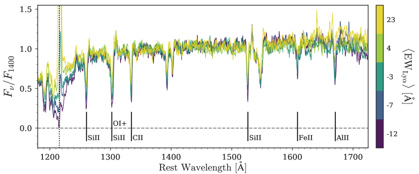
Figure 1: Stacked spectra of 703 galaxies sorted in quintiles of $\rm EW_{\mathrm{Ly}\alpha}$; the median $\rm EW_{\mathrm{Ly}\alpha}$ for each sample is given by the colorbar on the right. The dashed vertical line indicates Ly$\alpha$ while the solid vertical lines indicate the LIS transitions described in Table 2 and Sec. 3.2.2. The LIS line strengths vary similarly across all 6 distinct absorption features, such that strong LIS absorption is associated with weak Ly$\alpha$ emission and vice versa.

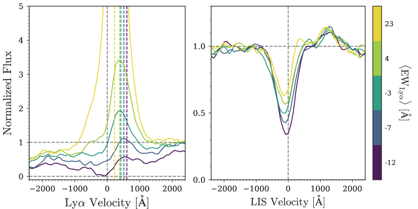
Figure 2: Stacked spectra in quintiles of $\rm EW_{\mathrm{Ly}\alpha}$, as in Fig. 1. The left panel is zoomed in on the Ly$\alpha$ line, and the dashed colored lines indicate the velocity of the Ly$\alpha$ centroid for each stacked subsample. The continuum for each stack is normalized at $\lambda_{\mathrm{rest}}=1400\,\textrm{\AA}$ as in Fig. 1. The right panel shows the combined LIS absorption profile for each stack, constructed by averaging the profiles of each of the LIS absorption features labeled in Fig. 1 according to the process described in Sec. 3.2.2 including normalization to the local continuum. Note that the stacked profiles show the same trends described in the text for individual objects: increased $\rm EW_{\mathrm{Ly}\alpha}$ is strongly associated with decreased (i.e., less redshifted) $v_{\mathrm{Ly}\alpha}$ and increased (i.e., weaker and less negative) $\rm EW_{\mathrm{LIS}}$.

2.3 MOSFIRE observations

The MOSFIRE observations for the KBSS-MOSFIRE survey are described in detail elsewhere (Steidel et al., 2014; Strom et al., 2017). Briefly, galaxies are observed in the $J$, $H$, and/or $K$ bands using 0$\farcs$7 slits, and the resulting two-dimensional spectrograms are reduced using the MOSFIRE data-reduction pipeline provided by the instrument team. Wavelength calibration is performed by identifying OH sky-lines in all spectral regions except in the red end of the $K$ band ($\lambda_{\mathrm{obs}}\gtrsim 2\,\textrm{$\mu$m}$), where arc lamp spectra are used due to the paucity of sky lines. The absolute flux scaling, slit-loss corrections, and cross-band calibration are performed through observations of a slit star on each mask, as discussed in detail by Strom et al. (2017). As described in that paper, the spatial extent of the KBSS galaxies (which are marginally resolved in typical atmospheric conditions) causes the slit losses for KBSS galaxies to exceed that measured directly from the slit star.

Line measurements are performed using the IDL program MOSPEC (Strom et al., 2017). Typically, galaxy redshifts and line fluxes are fit simultaneously in a single band ($J$, $H$, or $K$), with all nebular lines in the band constrained to have the same redshift and velocity width. For the [O III] $\lambda\lambda 4960,5008$ doublet, the known line flux ratio $f_{5008}/f_{4960}=3$ is also enforced. Line widths and redshifts are not forced to match between bands (e.g., for [O III] in the $H$ band and H$\alpha$ in the $K$ band, as would be observed at $z\approx 2-2.6$), but galaxies with redshift measurements in multiple bands are checked for consistency. Each galaxy is then assigned a nebular redshift $z_{\mathrm{neb}}$ based on the rest-frame optical redshift with the smallest uncertainty. For galaxies with redshift measurements in multiple bands, the typical agreement is less than $\Delta z=0.0002$.

2.4 SED models and SFRs

Photometry of the KBSS fields and spectral-energy distribution (SED) modeling of the KBSS galaxy sample is described by Steidel et al. (2014) and Strom et al. (2017) using SED-fitting methodology described by Reddy et al. (2012). Models are from the Bruzual & Charlot (2003) library and assume solar metallicity, a Chabrier (2003) initial mass function (IMF), a Calzetti et al. (2000) attenuation relation, and a constant star-formation history with a minimum age of 50 Myr. Stellar masses ($M_{*}$), star formation rates (SFR${}_{\text{SED}}$), and continuum-based reddening (E$(B-V)_{\rm{SED}}$) estimates are obtained from the SED fitting.

In addition to SED-based SFRs, H$\alpha$ SFRs are calculated for the majority of the KBSS-MOSFIRE sample as described by Strom et al. (2017) using the MOSFIRE measurements described above. These SFRs and sSFRs (sSFR = SFR${}_{\rm{H}\alpha}/M_{*}$) are calcuated assuming a Kennicutt (1998) H$\alpha$-SFR relation adjusted for a Chabrier (2003) IMF. Dust-corrections for H$\alpha$ SFRs are calculated as described in Sec. 3.2.3.

3 Empirical Galaxy Measurements

As described in Sec. 1, the primary goals of this paper are (1) to characterize the empirical relationships between Ly$\alpha$ emission and various other galaxy properties; and (2) to interpret these relationships in terms of the production and escape of Ly$\alpha$ photons. Below, we define the various observables used throughout this paper, and we categorize them in terms of whether they are likely to primarily relate to the production or escape of Ly$\alpha$ photons.

3.1 $\rm EW_{\mathrm{Ly}\alpha}$

First, we must define a metric of the efficiency of Ly$\alpha$ emission: the Ly$\alpha$ equivalent width ($\rm EW_{\mathrm{Ly}\alpha}$). We focus on $\rm EW_{\mathrm{Ly}\alpha}$ rather than the total Ly$\alpha$ luminosity for multiple reasons. Firstly, we find that the Ly$\alpha$ luminosity is primarily correlated with other descriptors of the total luminosity of a galaxy, so measuring the Ly$\alpha$ luminosity per unit UV continuum luminosity is a more interesting descriptor of the (in)ability of Ly$\alpha$ photons to escape relative to non-Ly$\alpha$ photons at similar wavelengths. Secondly, characterization of $\rm EW_{\mathrm{Ly}\alpha}$ is possible in slit spectra even without precise flux calibration, so our predictions for $\rm EW_{\mathrm{Ly}\alpha}$ can be more easily applied to actual observations of galaxies with uncertain slit losses.

The value of $\rm EW_{\mathrm{Ly}\alpha}$ is measured for each object in our sample directly from the one-dimensional object spectrum in a manner similar to that described in Trainor et al. (2015, 2016). Each rest-UV spectrum is first shifted to the rest frame based on its nebular redshift $z_{\mathrm{neb}}$. In order to account for the wide variety of Ly$\alpha$ line profiles in a systematic manner, the Ly$\alpha$ line flux, $F_{\mathrm{Ly}\alpha}$, was directly integrated by summing the continuum-subtracted line flux over the range $1208\,\textrm{\AA}<\lambda_{\mathrm{rest}}<1227\,\textrm{\AA}$, roughly the maximum range of wavelengths found to encompass the Ly$\alpha$ line in our spectra. In velocity space, this corresponds to a range $-1900\,\textrm{km}\,\textrm{s}^{-1}<v<2800\,\textrm{km}\,\textrm{s}^{-1}$ with respect to Ly$\alpha$. The local continuum flux $f_{\lambda,\mathrm{cont}}$ used for subtraction is estimated as the median flux in the range $1225\,\textrm{\AA}<\lambda_{\mathrm{rest}}<1250\,\textrm{\AA}$. The Ly$\alpha$ line flux $f_{\mathrm{Ly}\alpha}$ is therefore positive for net Ly$\alpha$ emission lines and negative for net Ly$\alpha$ absorption. The line flux and equivalent width are thus defined by the following expressions:

$$F_{\rm Ly\alpha} =\int_{1208\,\textrm{\AA}}^{1227\,\textrm{\AA}}\left(f_{\lambda}-f_{\lambda,\mathrm{cont}}\right)d\lambda$$ (1)

$$\rm EW_{\mathrm{Ly}\alpha} =\frac{F_{\mathrm{Ly}\alpha}}{f_{\lambda,\mathrm{cont}}}\frac{1}{1+z_{\mathrm{neb}}}\,\,.$$ (2)

Again, this procedure causes galaxies with net Ly$\alpha$ emission in their one-dimensional slit spectra to have $\rm EW_{\mathrm{Ly}\alpha}>0$, and galaxies exhibiting net Ly$\alpha$ absorption to be assigned $\rm EW_{\mathrm{Ly}\alpha}<0$. Note that, in each case, the assigned value of $\rm EW_{\mathrm{Ly}\alpha}$ is likely to be an underestimate of the the intrinsic value owing to the spatial scattering of Ly$\alpha$ photons, which preferentially lowers the observed ratio of Ly$\alpha$ photons to continuum photons in a centralized aperture. Typical relative slit losses of Ly$\alpha$ respect to the nearby continuum in similar samples are found to be $2-3\times$ (see, e.g., Steidel et al. 2011; Trainor et al. 2015). However, we have no way to determine the relative Ly$\alpha$ slit loss for the majority of individual objects in our sample, so we do not attempt to do so here. Furthermore, in this work we are primarily concerned with the factors that determine the net Ly$\alpha$ emission on galaxy scales; variation in the total Ly$\alpha$ emission of the galaxy-plus-halo system with physical and environmental properties of the galaxies will be discussed in future work.

Uncertainty in $\rm EW_{\mathrm{Ly}\alpha}$ is determined based on the uncertainty in the Ly$\alpha$ flux (usually a small factor) as well as the uncertainty in the local continuum (usually the dominant factor, particularly for high-$\rm EW_{\mathrm{Ly}\alpha}$ sources). In some cases, correlated noise in the continuum spectrum causes the formal uncertainty in the local continuum to be unrealistically low based on a visual inspection of the spectrum. To account for this fact, a separate estimate of the continuum flux $f_{\lambda,\mathrm{cont}}$ is measured for each galaxy over the range $1220\,\textrm{\AA}<\lambda_{\mathrm{rest}}<1300\,\textrm{\AA}$ (i.e., over a $\sim$3$\times$ larger range of wavelengths than the first estimate), and this second continuum estimate is used to recalculate $F_{\mathrm{Ly}\alpha}$ and $\rm EW_{\mathrm{Ly}\alpha}$. If the new $\rm EW_{\mathrm{Ly}\alpha}$ value differs from the original value by more than the uncertainty on $\rm EW_{\mathrm{Ly}\alpha}$ calculated originally, then the uncertainty on $\rm EW_{\mathrm{Ly}\alpha}$ is replaced by the absolute value of the difference between the two estimates of $\rm EW_{\mathrm{Ly}\alpha}$. This procedure increases the uncertainty on $\rm EW_{\mathrm{Ly}\alpha}$ for 59 objects (8% of the total sample), and the total variance in $\rm EW_{\mathrm{Ly}\alpha}$ associated with our estimated measurement error among our entire sample increases by 5%.

Furthermore, if the measured continuum value is smaller than $2\times$ the estimated uncertainty on the continuum, then $\rm EW_{\mathrm{Ly}\alpha}$ is defined to be a lower limit:

$$\rm EW_{\mathrm{Ly}\alpha}>\frac{F_{\mathrm{Ly}\alpha}}{2\sigma_{\lambda,\mathrm{cont}}}\frac{1}{1+z_{\mathrm{neb}}}$$ (3)

where $\sigma_{\lambda,\mathrm{cont}}$ is the formal uncertainty in the local Ly$\alpha$ continuum. This correction applies to 13 objects (2% of our total sample), and $\rm EW_{\mathrm{Ly}\alpha}$ for these objects is assumed to take the value of their 2$\sigma$ error in the analysis that follows. In this manner, a value and uncertainty for $\rm EW_{\mathrm{Ly}\alpha}$ is estimated for each of the 703 galaxies in our sample.

Spearman rank correlation statistics between $\rm EW_{\mathrm{Ly}\alpha}$ and a series of other empirical quantities measured among the galaxies in our sample are given in Table 1 below. Definitions and measurement methodologies for each of these quantities are given in the sections that follow.

3.2 Proxies for Ly$\alpha$ escape

3.2.1 $v_{\mathrm{Ly}\alpha}$

As discussed in Sec. 1 above, increasing shifts of the Ly$\alpha$ emission line with respect to the systemic redshift are associated with decreasing $\rm EW_{\mathrm{Ly}\alpha}$, and this trend likely corresponds to the fact that Ly$\alpha$ photons must scatter significantly in redshift and/or physical space to escape regions of high optical depth. For this reason, the difference of the Ly$\alpha$ redshift ($z_{\rm Ly\alpha}$) from systemic ($z_{\mathrm{neb}}$) may be regarded as a proxy for the optical depth experienced by Ly$\alpha$ photons transiting the galaxy ISM and CGM and is thus related to the probability of Ly$\alpha$ photon escape.

We define the Ly$\alpha$ redshift and offset velocity based on the centroid of the Ly$\alpha$ line flux:

Table 1: Correlations

Quantities			$N_{\mathrm{gal}}$	$r_{\mathrm{Sp}}$	$\log_{10}(p)$
Escape-related quantities
EWLyα	vs.	$v_{\mathrm{Ly}\alpha}$	496	$-$0.56	$-$41.8
	vs.	EWLIS	669	0.35	$-$20.5
	vs.	E($B-V$)SED	637	$-$0.23	$-$8.2
	vs.	E($B-V$)neb	208	$-$0.14	$-$1.3
EWLIS	vs.	$v_{\mathrm{Ly}\alpha}$	479	0.28	$-$9.5
	vs.	$f_{\mathrm{esc,rel}}$	368	$-$0.42	$-$16.5
	vs.	$f_{\mathrm{esc,abs}}$	188	$-$0.50	$-$12.4
Production-related quantities
EWLyα	vs.	$M_{*,\rm{SED}}$	637	$-$0.15	$-$3.9
	vs.	SFRSED	637	$-$0.17	$-$5.0
	vs.	SFRHα	208	$-$0.05	$-$0.4
	vs.	sSFRHα	199	0.23	$-$3.0
	vs.	$M_{\rm{UV}}$	637	$-$0.01	$-$0.1
	vs.	O32raw	316	0.43	$-$15.0
	vs.	O32corr	174	0.47	$-$10.3
	vs.	O3	395	0.40	$-$15.3
Production + escape
EWLIS	vs.	O3	377	0.21	$-$4.9
	vs.	O32corr	174	0.47	$-$10.3
EWLyα	vs.	$X_{\mathrm{LIS}}^{\mathrm{O3}}$	377	0.49	$-$23.8

$$\lambda_{\rm Ly\alpha}^{\rm obs} =\frac{\int\lambda f_{\lambda}d\lambda}{\int f_{\lambda}d\lambda}$$ (4)

$$z_{\rm Ly\alpha} =\frac{\lambda_{\rm Ly\alpha}^{\rm obs}-\lambda_{\rm Ly\alpha}^{\rm rest}}{\lambda_{\rm Ly\alpha}^{\rm rest}}$$ (5)

$$v_{\mathrm{Ly}\alpha} =\left(\frac{z_{\rm Ly\alpha}-z_{\rm neb}}{1+z_{\rm neb}}\right)\rm{c}$$ (6)

where c is the speed of light and the integrals in Eq. 4 are evaluated over the range $1208\,\textrm{\AA}<\lambda_{\mathrm{rest}}<1227\,\textrm{\AA}$, as is done to estimate the total Ly$\alpha$ flux (Eq. 1). Note, however, that in this case we integrate the raw flux over the Ly$\alpha$ region rather than integrating the continuum-subtracted flux. This choice does not appreciably change the assigned value of $v_{\mathrm{Ly}\alpha}$ when $\rm EW_{\mathrm{Ly}\alpha}$ is large, but it significantly reduces the noise on $v_{\mathrm{Ly}\alpha}$ when $\rm EW_{\mathrm{Ly}\alpha}\to 0$, in which case the denominator would approach zero for an analogous equation to Eq. 4 weighted by continuum-subtracted flux.

Note also that the flux in the Ly$\alpha$ transition need not exceed $f_{\lambda,\mathrm{cont}}$ in order to measure a Ly$\alpha$ velocity; if a galaxy exhibits Ly$\alpha$ absorption that is preferentially blueshifted, the assigned Ly$\alpha$ velocity will be positive and thus similar to a galaxy with redshifted Ly$\alpha$ emission.

Velocity uncertainties are determined by a Monte Carlo analysis in which a randomly-generated error array consistent with the per-pixel uncertainty is added to the Ly$\alpha$ region of the spectrum and the velocity is measured as above. This process is repeated 1000 times per spectrum, and the estimated velocity uncertainty is 1.5$\times$ the median absolute deviation of the Monte Carlo velocity values. While velocity measurements can be made in this way for every spectrum in our sample, we include in our analysis of $v_{\mathrm{Ly}\alpha}$ only those spectra with a Ly$\alpha$ velocity uncertainty $\sigma_{\rm Ly\alpha}<750\,\,\textrm{km}\,\textrm{s}^{-1}$. Because the Ly$\alpha$ velocity also depends on the accuracy of $z_{\rm neb}$, we also require that H$\alpha$ and/or [O III] $\lambda 5008$ are detected with at least 5$\sigma$ significance. When these cuts are made, 496 galaxies in our sample have reliably measured values of $v_{\mathrm{Ly}\alpha}$. The Spearman rank correlation statistic between $v_{\mathrm{Ly}\alpha}$ and $\rm EW_{\mathrm{Ly}\alpha}$ is $r_{\rm Sp}=-0.56$ ($p=1.6\times 10^{-42}$), indicating a strong, highly-significant correlation. This relationship is consistent with previous work (e.g., Erb et al. 2014) as well as our results from stacked spectra shown in Fig. 2 (left panel).

As described in Sec. 1, our eventual goal is to predict the value of $\rm EW_{\mathrm{Ly}\alpha}$ for a galaxy in the absence of its direct measurement (since the Ly$\alpha$ flux is not always directly observable). Unfortunately, $v_{\mathrm{Ly}\alpha}$ may be ineffective as such a predictor for two reasons. Firstly, $v_{\mathrm{Ly}\alpha}$ cannot be measured in cases where Ly$\alpha$ is not directly measurable (e.g., when the transition is censored by the IGM or contaminated by other emission). Secondly, even in cases where $v_{\mathrm{Ly}\alpha}$ is measurable (e.g., among some galaxies at high redshift), any intergalactic absorption that suppresses $\rm EW_{\mathrm{Ly}\alpha}$ is also likely to change the observed value of $v_{\mathrm{Ly}\alpha}$. Because scattering of Ly$\alpha$ by both the ISM and the surrounding IGM will produce degenerate shifts on $v_{\mathrm{Ly}\alpha}$, $v_{\mathrm{Ly}\alpha}$ itself cannot be expected to separate between these two effects. With this in mind, we caution against the use of $v_{\mathrm{Ly}\alpha}$ to predict the intrinsic value of $\rm EW_{\mathrm{Ly}\alpha}$.

3.2.2 $\rm EW_{\mathrm{LIS}}$

The second proxy we use for the ease of Ly$\alpha$ photon escape is the strength of absorption lines corresponding to low-ionization interstellar gas. Unfortunately, even the strongest interstellar absorption features are difficult to measure reliably in individual spectra. In order to increase the significance of these detections, we construct a “mean” LIS absorption profile for each galaxy spectrum as follows.

Table 2: LIS Transitions

Ion	$\lambda_{\textrm{\scriptsize{vac}}}$ (Å)	$f_{\textrm{\scriptsize{osc}}}$	xEW${}_{\textrm{\scriptsize{ion}}}$ (Å)
Si II	1260.418	1.22	$1.74\pm 0.06$
O I	1302.169	0.0520	$2.37\pm 0.08$
Si II	1304.370	0.0928	$2.37\pm 0.08$
C II	1334.532	0.129	$1.54\pm 0.08$
Si II	1526.707	0.133	$1.40\pm 0.10$
Fe II	1608.451	0.0591	$1.11\pm 0.14$
Al II	1670.787	1.77	$1.13\pm 0.21$

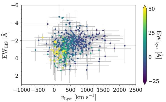
Figure 3: Centroid Ly$\alpha$ velocity vs. rest-frame equivalent width of LIS absorption for 452 galaxies, with colors denoting Ly$\alpha$ equivalent width. Two clear trends are visible: (1) stronger LIS absorption (EW${}_{\mathrm{LIS}}<$0) is associated with increasing Ly$\alpha$ redshift ($v_{\mathrm{Ly}\alpha}>0$); and (2) strong Ly$\alpha$ emission (EW${}_{\mathrm{Ly}\alpha}>0$, yellow points) is associated with both weak LIS absorption and small Ly$\alpha$ redshifts.

Seven LIS transitions covered by the majority of our rest-UV spectra are identified in Table 2. O I $\lambda 1302$ and Si II $\lambda 1304$ are blended at the typical spectral resolution of our observations, so six distinct absorption features can be individually measured. For each transition, the spectral region within $\pm 5000\,\textrm{km}\,\textrm{s}^{-1}$ of the rest-frame wavelength is interpolated onto a grid in velocity space and normalized to its local continuum (defined as the median flux in the region $>$$1000\,\textrm{km}\,\textrm{s}^{-1}$ and $<$$5000\,\textrm{km}\,\textrm{s}^{-1}$ from the transition wavelength in either direction). The six LIS absorption profiles are then averaged with equal weighting, and an effective rest-frame equivalent width in absorption is measured for the stacked profile via direct integration according to the following expression, which we define as $\rm EW_{\mathrm{LIS}}$:

$$\rm EW_{\mathrm{LIS}} =\int_{\lambda_{1}}^{\lambda_{2}}\left(1-\frac{f_{\lambda}}{f_{\mathrm{cont}}}\right)d\lambda$$ (7)

where $\lambda_{1}$ and $\lambda_{2}$ correspond to $\pm 1000\,\textrm{km}\,\textrm{s}^{-1}$ from the rest-frame line center. The uncertainty on $\rm EW_{\mathrm{LIS}}$ is defined to be the standard deviation of absorption equivalent widths calculated as above for random $2000\,\textrm{km}\,\textrm{s}^{-1}$ intervals in nearby regions of the rest-UV spectrum. Because the reliability of our $\rm EW_{\mathrm{LIS}}$ measurement is extremely sensitive to the strength of the FUV continuum, we only consider measurements of $\rm EW_{\mathrm{LIS}}$ for which the local continuum is detected with S/N $>20$ in the stacked profile; this sample includes 625 objects.

For 162 objects in this sample, one or more LIS transitions fall above the red edge of the LRIS-B spectrum. For 19 objects, one or more LIS transitions are flagged as discrepant: they either correspond to a EW more than $15\sigma$ away from the median EW of the other transitions, or they otherwise lie in a region of the spectrum that appears significantly noisier than average based on a visual inspection. In any of these cases, the missing or flagged transitions are omitted, and the mean $\rm EW_{\mathrm{LIS}}$ value and uncertainty are calcuated from the remaining transitions. In total, the number of objects for which 6 (5, 4, 3, 2, 1) transitions contribute to $\rm EW_{\mathrm{LIS}}$ is 456 (75, 56, 42, 8, 0).

As described above, the vast majority of cases where one or more transitions are omitted occur because of a lack of red spectral coverage, such that the redder transitions in Table 2 are preferentially omitted. Given that the two strongest transitions are also the two bluest (and thus, least likely to be omitted), there is potential for our spectral coverage to introduce a trend between $\rm EW_{\mathrm{LIS}}$ and the number of included transitions. Separating galaxies by the number of included LIS transitions ($N_{\mathrm{LIS}}$), the median value of $\rm EW_{\mathrm{LIS}}$ for each subset is (1.43Å, 1.49Å, 1.27Å, 1.40Å, 1.55Å) for $N_{\mathrm{LIS}}=($6, 5,4, 3, 2$)$. The lack of a systematic trend between $\rm EW_{\mathrm{LIS}}$ and $N_{\mathrm{LIS}}$ suggests that our $\rm EW_{\mathrm{LIS}}$ values are not particularly sensitive to the precise subset of LIS transitions included.

The distribution of $\rm EW_{\mathrm{LIS}}$ vs. $v_{\mathrm{Ly}\alpha}$ is shown in Fig. 3 for the 479 objects for which both quantities are measured robustly according to the criteria described above. The Spearman correlation coefficient for these two parameters is $r_{\rm Sp}=0.28$ ($p=3.2\times 10^{-10}$; see Table 1), indicating a moderate (although highly statistically significant) correlation between these two proxies for ISM optical depth (or porosity) and the likely ease of Ly$\alpha$ photon escape. The color-coding by $\rm EW_{\mathrm{Ly}\alpha}$ in Fig. 3 demonstrates that strong Ly$\alpha$ emission is associated with weak LIS absorption and a small shift of the Ly$\alpha$ line with respect to systemic, in agreement with the expectations outlined above. The correlation between $\rm EW_{\mathrm{LIS}}$ and $\rm EW_{\mathrm{Ly}\alpha}$ is moderately strong and highly significant ($r_{\rm Sp}=-0.35$, $p=3\times 10^{-21}$).

We note that $\rm EW_{\mathrm{LIS}}$ has multiple practical advantages over $v_{\mathrm{Ly}\alpha}$ as a predictor of $\rm EW_{\mathrm{Ly}\alpha}$. Unlike $v_{\mathrm{Ly}\alpha}$, $\rm EW_{\mathrm{LIS}}$ is likely to be unaffected by IGM absorption, since the metallicity of intergalactic gas will be negligible compared to that of the enriched galactic outflows traced by metal-line absorption. In addition, in the event that the Ly$\alpha$ transition is censored by the IGM, local H I or contaminating emission, the longer-wavelength LIS transitions may still be measurable in many realistic cases at both low and high redshifts. For these reasons, our analysis that follows utilizes $\rm EW_{\mathrm{LIS}}$ as our primary proxy for Ly$\alpha$ escape.

3.2.3 E($B-V$)

Because the escape of Ly$\alpha$ photons depends on the distribution of dust in galaxies as well as H I, we also consider the relationship between $\rm EW_{\mathrm{Ly}\alpha}$ and E($B-V$) (see also discussion in Trainor et al. 2016 and Theios et al. 2019).

E($B-V$)_SED is measured via SED-fitting as described in Sec. 2.4 for 637 galaxies. Comparing these values to $\rm EW_{\mathrm{Ly}\alpha}$ yields a moderate, highly-signficant correlation ($r_{\rm Sp}=-0.23$, $p=3\times 10^{-8}$).

We also measure E($B-V$)_neb based on the Balmer decrement (H$\alpha$/H$\beta$) as described by Strom et al. (2017). Briefly, the slit-loss-corrected H$\alpha$ and H$\beta$ fluxes are compared to the canonical ratio H$\alpha$/H$\beta$ = 2.86 for Case-B recombination at $T=10^{4}$ K (Osterbrock, 1989). Galaxies with H$\alpha$/H$\beta$ $<2.86$ are assigned E($B-V$)_neb = 0, while galaxies with H$\alpha$/H$\beta$ $>2.86$ are assigned a value of E($B-V$)_neb based on a Cardelli et al. (1989) Galatic attenuation relation. The median value of E($B-V$)_neb for KBSS galaxies is 0.26, and the interquartile range is 0.06$-$0.47(Strom et al., 2017).

As discussed by Trainor et al. (2016) and Strom et al. (2017), the H$\beta$ and H$\alpha$ emission lines are measured in separate exposures in KBSS-MOSFIRE observations; at typical redshifts $2.0<z<2.6$, the lines fall in the $H$ and $K$ NIR atmospheric bands, respectively. For this reason, we present values of E($B-V$)_neb only for those galaxies with $>$5$\sigma$ measurements of H$\alpha$/H$\beta$ including the uncertainties in the individual line fluxes as well as the cross-band calibration. This cut limits our sample of secure E($B-V$)_neb measurements to 208 galaxies, which display a weak correlation with $\rm EW_{\mathrm{Ly}\alpha}$ ($r_{\rm Sp}=-0.14$, $p=0.05$).

3.2.4 $f_{\mathrm{esc}}$

The most direct measure of the efficiency of Ly$\alpha$ photon escape is the actual escape fraction of Ly$\alpha$, hereafter $f_{\mathrm{esc}}$. Any determination of this escape fraction relies on an estimation of the true number of Ly$\alpha$ photons produced in galaxies, which can then be compared to the observed Ly$\alpha$ flux. In practice, the observed Ly$\alpha$ flux is compared to the observed H$\alpha$ flux, with the latter value scaled by the expected intrinsic flux ratio $\left(F_{\mathrm{Ly}\alpha}/F_{\mathrm{H}\alpha}\right)_{\mathrm{int}}\approx 8.7$ for case-B recombination.

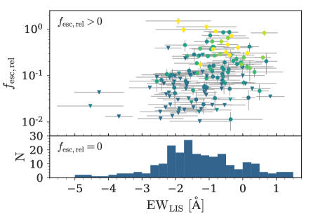
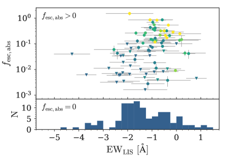
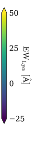
Figure 4: The Ly$\alpha$ photon escape fraction vs. the rest-frame equivalent width of LIS absorption, with color coding by Ly$\alpha$ equivalent width. Circles indicate formal detections, while triangles indicate 2$\sigma$ upper limits on $f_{\mathrm{esc}}$. The left panel gives the escape fraction of Ly$\alpha$ photons relative to H$\alpha$ (Eq. 8) for 368 galaxies with detected Ly$\alpha$ and H$\alpha$ emission. The right panel gives the absolute escape fraction of Ly$\alpha$ photons (Eq. 9) for 188 galaxies that also have robust estimates of the Balmer decrement (used to dust-correct the H$\alpha$ flux). Bottom panels show the EW_LIS distribution for galaxies with $F_{\mathrm{Ly}\alpha}<0$.

H$\alpha$ provides an effective proxy for the intrinsic Ly$\alpha$ luminosity because the former is not significantly scattered by H I; however, it nonetheless suffers extinction by interstellar dust. The intrinsic H$\alpha$ flux (and thus, the instrinsic Ly$\alpha$ flux) can therefore only be determined using the absolute attenuation $A_{\mathrm{H}\alpha}$, which is typically estimated from the inferred nebular reddening (i.e., E($B-V$) as defined in Sec. 3.2.3) and the application of an attenuation relation that is appropriate to the galaxy at hand. As discussed by Theios et al. (2019), no single attenuation relation is able to self-consistently describe the host of photometric and spectroscopic properties inferred for KBSS galaxies. Given these ambiguities in the attenuation correction, we present both the relative (i.e., dust-uncorrected) and absolute (i.e., dust-corrected) Ly$\alpha$ escape fractions based on the following definitions:

$$f_{\rm esc,rel} =\frac{F_{\rm Ly\alpha}}{8.7\times F_{\rm H\alpha,obs}}$$ (8)

$$f_{\rm esc,abs} =\frac{F_{\rm Ly\alpha}}{8.7\times F_{\rm H\alpha,corr}}$$ (9)

where $F_{\rm H\alpha,obs}$ is the observed H$\alpha$ flux and $F_{\rm H\alpha,corr}$ is that corrected based on the observed E($B-V$)_neb and the application of a Cardelli et al. (1989) attenuation relation. In both cases, $F_{\rm Ly\alpha}$ is the observed Ly$\alpha$ flux as defined in Eq. 1, which is not dust-corrected.

We calculate $f_{\rm esc,rel}$ via Eq. 8 for 368 galaxies for which we have a 5$\sigma$ detection of H$\alpha$ (we take $f_{\rm esc,rel}=0$ where $F_{\rm Ly\alpha}\leq 0$) as well as a measurement of $\rm EW_{\mathrm{LIS}}$. As described in Sec. 3.2.3, only 208 galaxies have a robust measurement of E($B-V$)_neb; when combined with the S/N cuts on H$\alpha$ and $\rm EW_{\mathrm{LIS}}$, this leaves 188 galaxies for which $f_{\rm esc,abs}$ may be calculated with confidence via Eq. 9 (although subject to the remaining uncertainty in the attenuation law as well as differential slit losses in Ly$\alpha$ vs. H$\alpha$).

Fig. 4 displays the relationship between $\rm EW_{\mathrm{LIS}}$ and $f_{\rm esc}$ in both its absolute and relative forms. In either case, the two quantities have a relatively strong correlation given the measurement uncertainties ($r_{\rm Sp}=-0.50$, $p=6\times 10^{-13}$ for 188 galaxies for $f_{\rm esc,abs}$; Table 1). Again, our analysis that follows is restricted to using $\rm EW_{\mathrm{LIS}}$ as a proxy for Ly$\alpha$ escape because $f_{\rm esc}$, like $v_{\mathrm{Ly}\alpha}$, is not typically measurable in cases where we would like to predict $\rm EW_{\mathrm{Ly}\alpha}$.

3.3 Proxies for Ly$\alpha$ production

3.3.1 SFR, Mass, and Luminosity

We now consider parameters that may be associated with Ly$\alpha$ production. As noted above, H$\alpha$ luminosity should be a fairly direct proxy for the intrinsic luminosity of a galaxy in Ly$\alpha$. However, it is less related to the efficiency of Ly$\alpha$ production as described by $\rm EW_{\mathrm{Ly}\alpha}$: dust-corrected $L_{\rm H\alpha}$ is uncorrelated with $\rm EW_{\mathrm{Ly}\alpha}$  in our sample ($r_{\rm Sp}=-0.05$, $p=0.4$) for the 208 galaxies with robust estimations of E($B-V$) and $A_{\rm{H}\alpha}$ (see Sec. 3.2.3); the same correlation holds between $\rm EW_{\mathrm{Ly}\alpha}$ and SFR_Hα since SFR_Hα is linearly related to $L_{\rm{H}\alpha}$.

Our photometry-based estimates of SFR_SED display slightly stronger relationships with $\rm EW_{\mathrm{Ly}\alpha}$ ($r_{\rm Sp}=-0.17$, $p=10^{-5}$), and the correlation for stellar mass is very similar ($r_{\rm Sp}=-0.15$, $p=10^{-4}$) for the 637 galaxies with SED fits and $\rm EW_{\mathrm{Ly}\alpha}$ measurements. sSFR (SFR_Hα/$M_{*}$) displays a slightly stronger correlation with $\rm EW_{\mathrm{Ly}\alpha}$ ($r_{\rm Sp}=0.23$, $p=10^{-3}$) with lower significance due to the smaller sample size of objects with the necessary measurements of both SFR_Hα and $M_{*}$ (199 galaxies).

Rest-UV absolute magnitudes M_UV are measured from the $G$ and $\mathcal{R}$ band magnitudes. The apparent magnitude corresponding to a rest-frame wavelength $\lambda_{\text{rest}}=1450$Å is estimated by taking a weighted average of the $G$ and $\mathcal{R}$ based on the redshift of the galaxy. This apparent magnitude $m_{\text{UV}}$ is then converted to the absolute magnitude $M_{\text{UV}}$ based on the redshift of the source and the luminosity distance calculated assuming a $\Lambda$CDM cosmological model with $H_{0}=70\,\mathrm{km}\,\mathrm{s}^{-1}\,\mathrm{Mpc}^{-1}$, $\Omega_{m}=0.3$, and $\Omega_{\Lambda}=0.7$. In this manner, M_UV is measured for each of the 637 galaxies in our SED-fit sample. This parameter shows the weakest relationship with $\rm EW_{\mathrm{Ly}\alpha}$ of any quantity we measure, with $r_{\rm Sp}=-1.5\times 10^{-2}$ and $p=0.71$. This lack of association between UV luminosity and $\rm EW_{\mathrm{Ly}\alpha}$ is remarkable given the high $\rm EW_{\mathrm{Ly}\alpha}$ values associated with faint, high-$z$ galaxies in other recent work; these trends are discussed further in Sec. 6.

3.3.2 O32

By definition, the intrinsic $\rm EW_{\mathrm{Ly}\alpha}$ of a galaxy is the ratio of Ly$\alpha$ photons to UV continuum photons, where the latter are generated directly by OB stars and the former are generated by the gas excited and ionized by these same stars. It is therefore sensible that $\rm EW_{\mathrm{Ly}\alpha}$ would be strongly associated with the excitation and ionization states of the gas in star-forming regions.

The O32 line ratio is one commonly-used indicator of nebular ionization (Sanders et al., 2016; Steidel et al., 2016; Strom et al., 2017, 2018):

$$\text{O32}\equiv\log\left(\frac{[\text{O III}]\,\lambda\lambda 4960,5008}{[\text{O II}]\,\lambda\lambda 3727,3729}\right)$$ (10)

For the ionization-bounded H II regions typically assumed in photoionization models of star-forming galaxies, O32 is approximately proportional to log($U$), where $U$ denotes the “ionization parameter”, the local number of hydrogen-ionizing photons per hydrogen atom. (see discussion by Steidel et al. 2016). Furthermore, O32 has previously been found to correlate strongly with Ly$\alpha$ emission (e.g., Trainor et al. 2016; Nakajima et al. 2016).

Notably, however, recent work has suggested that elevated O32 values may correspond in some cases to density-bounded H II regions, in which the ionized region is not entirely surrounded by neutral gas (Nakajima et al., 2013; Trainor et al., 2016; Izotov et al., 2016). In particular, several recent detections of escaping Ly-continuum (rest-frame H ionizing) photons from galaxies at low and high redshift have been accompanied by elevated O32 ratios (e.g., de Barros et al. 2016; Izotov et al. 2016, 2018; Fletcher et al. 2018, but c.f. Borthakur et al. 2014 and Shapley et al. 2016 who find Ly-continuum escape in the absense of extreme O32). In these scenarios, an association of large O32 with high $\rm EW_{\mathrm{Ly}\alpha}$ may reflect a combination of both increased ionizing photon production and increased probability of photon escape due to the lack of surrounding neutral gas.

O32 measurements for the KBSS sample are calculated as described in Strom et al. (2017). Briefly, the [O III] $\lambda\lambda$4960,5008 and [O II] $\lambda\lambda$3727,3729 line fluxes are measured as described in Sec. 2.3. We require that both [O III] and [O II] be detected with S/N $>3$, resulting in a sample of 316 galaxies with a measured raw O32 value. Dust-corrected O32 values are measured for a smaller sample of 174 objects that meet both the requirements described above as well as the cut on the S/N of the Balmer decrement described in Sec. 3.2.4. For these measurements, each of the [O III] and [O II] emission lines are corrected for extinction using the measured Balmer decrement and a Cardelli et al. (1989) attenuation curve before calculating the line ratio. These two O32 estimators have the highest individual correlations with $\rm EW_{\mathrm{Ly}\alpha}$ of any “production”-related parameter: $r_{\rm Sp}=0.43$ ($p=10^{-15}$) for the raw O32 measurements with a slightly higher correlation strength and lower significance for the smaller sample of dust-corrected O32 values (Table 1). However, O32 also displays a strong correlation with $\rm EW_{\mathrm{LIS}}$ ($r_{\rm Sp}=0.47$), perhaps reinforcing the idea that O32 is not wholly a measure of Ly$\alpha$ production.

3.3.3 O3

The O3 ratio is another indicator of nebular ionization and excitation:

$$\text{O3}\equiv\log\left(\frac{[\text{O III}]\,\lambda 5008}{\text{H}\beta}\right)\quad.$$ (11)

As discussed by Trainor et al. (2016), the O3 ratio is strongly associated with O32 for the high-excitation galaxies typical at $z\gtrsim 2$: the two quantities are correlated with $r_{\rm Sp}=0.74$ in the KBSS sample. Likewise, Strom et al. (2018) demonstrate that O3 is an effective indicator of log($U$) through extensive photoionization modeling of the KBSS galaxy sample. O3 therefore has many of the same advantages as O32 for indicating Ly$\alpha$ production.

However, O3 has two significant advantages over O32. Firstly, O3 relies on two emission lines at similar wavelengths, which makes the ratio insensitive to both dust extinction and cross-band calibration. Secondly, O3 is insensitive to the differences between density-bounded and ionization-bounded H II regions, so it may indicate nebular excitation (and Ly$\alpha$ production) in a manner more decoupled from the physics of Ly$\alpha$ escape. Based on these advantages, we rely on O3 as our primary metric of Ly$\alpha$ production efficiency for the remainder of this work.

Using the same line-fitting process described above to estimate the line fluxes and uncertainties, we calculate the O3 ratio for every galaxy that has S/N $>3$ for both [O III] and H$\beta$, a total of 395 objects. O3 has a correlation with $\rm EW_{\mathrm{Ly}\alpha}$ that is only marginally weaker than the corresponding correlation for O32 ($r_{\rm Sp}=0.40$, $p=5\times 10^{-16}$).

3.4 Summary of correlations with Ly$\alpha$

Again, Spearman rank correlation statistics for $\rm EW_{\mathrm{Ly}\alpha}$ and $\rm EW_{\mathrm{LIS}}$ with other measured quantities are presented in Table 1. Each quantity is calculated for a different number of objects according to the cuts described above, and the $p$ values of every measured correlation (which depend both on the measured $r$ and the number of objects in the sample) are highly significant ($p\ll 1$ in nearly all cases). However, there is a wide range of $r$ values, indicating that certain parameters explain only a small fraction in the total variation in $\rm EW_{\mathrm{Ly}\alpha}$ despite the statistical significance of their correlation.

Note that $\rm EW_{\mathrm{LIS}}$ is strongly correlated with the escape fraction of Ly$\alpha$  as expected based on the arguments that both of these quantities are related to the ability of Ly$\alpha$ photons to escape galaxies (see Sec. 3.2.2 and Fig. 4). Conversely, $\rm EW_{\mathrm{LIS}}$ has a much weaker correlation with O3 despite the fact that both quantities show relatively strong correlations with $\rm EW_{\mathrm{Ly}\alpha}$. We interpret this relationship in the sections that follow, but it is suggestive of the fact that these two quantities capture different processes (escape and production) related to the observed $\rm EW_{\mathrm{Ly}\alpha}$.

Figure 5: O3 ratio ($\equiv\log($[O III]/H$\beta$$)$) vs. rest-frame equivalent width of LIS absorption for 377 galaxies, with colors denoting Ly$\alpha$ equivalent width. Note that O3 and EW_LIS are not strongly correlated with each other, but EW${}_{\mathrm{Ly}\alpha}>0$ is strongly associated with both weak LIS absorption (EW${}_{\mathrm{LIS}}\approx 0$) and strong [O III] emission (O3 $\gtrsim 0.5$). Square boxes with black borders correspond to stacked measurements of faint $L\sim 0.1L_{*}$ Ly$\alpha$-selected galaxies from Trainor et al. (2015, 2016). The large square denotes the full sample, and the smaller squares denote measurements based on splitting about the median value of $\rm EW_{\mathrm{Ly}\alpha}$. Diamond with black border represents MS 1512-cB58 based on measurements from Pettini et al. (2002) and Teplitz et al. (2000).

Fig. 5 visually demonstrates this same result. While O3 and $\rm EW_{\mathrm{LIS}}$ are themselves not closely correlated, there is a clear trend toward high $\rm EW_{\mathrm{Ly}\alpha}$ in the upper-right corner of Fig. 5 (i.e., the region of high O3 and/or $\rm EW_{\mathrm{LIS}}$ $\sim$ 0) and low $\rm EW_{\mathrm{Ly}\alpha}$ in the lower-left corner (i.e., the region of low O3 and/or strongly-negative $\rm EW_{\mathrm{LIS}}$).

Fig. 5 also includes measurements from stacked spectra of faint $L\sim 0.1L_{*}$ Ly$\alpha$-selected galaxies from the KBSS-Ly$\alpha$ survey; these measurements are shown as boxed points. The $\rm EW_{\mathrm{LIS}}$ measurements are described by Trainor et al. (2015), while the O3 measurements are described by Trainor et al. (2016). The faint galaxy measurements follow the same trend as the individual measurements from the brighter KBSS galaxies, in that high $\rm EW_{\mathrm{Ly}\alpha}$ is associated with the upper-right corner of the parameter space.

For comparison, we also include measurements of MS 1523-cB58, a gravitationally lensed galaxy with $M_{*}\approx 10^{9}$ $\rm M_{\odot}$, SFR $\approx 50-100$ $\rm M_{\odot}$ yr^-1, and a young age $\sim$9 Myr (Siana et al., 2008). The reported O3 value is based on spectroscopic measurements reported by Teplitz et al. (2000), while the Ly$\alpha$ and LIS equivalent widths are new measurements from the Keck/ESI spectrum presented by Pettini et al. (2002). Despite its young age and large star-formation rate – both of which would predict a high rate of Ly$\alpha$ production – the spectrum of MS 1512-cB58 (hereafter cB58) displays net Ly$\alpha$ absorption, consistent with its deep LIS absorption lines ($\rm EW_{\mathrm{LIS}}$ $\approx-3$Å). The galaxy cB58 thus obeys the same association as the KBSS galaxies between Ly$\alpha$ emission and position in the O3-$\rm EW_{\mathrm{LIS}}$ parameter space.

The structure of Fig. 5 therefore suggests that a linear combination of O3 and $\rm EW_{\mathrm{LIS}}$ would better predict $\rm EW_{\mathrm{Ly}\alpha}$ than either quantity alone. That is, we could in principle define a single parameter which is maximized when both O3 and $\rm EW_{\mathrm{LIS}}$ predict strong $\rm EW_{\mathrm{Ly}\alpha}$, is minimized when both O3 and $\rm EW_{\mathrm{LIS}}$ predict weak $\rm EW_{\mathrm{Ly}\alpha}$, and which takes intermediate values when O3 and $\rm EW_{\mathrm{Ly}\alpha}$ have contradictory implications for the value of $\rm EW_{\mathrm{Ly}\alpha}$. We develop such a model in Sec. 4 below.

4 Combined Model

Motivated by the arguments above, we construct a new parameter $X_{\mathrm{LIS}}^{\mathrm{O3}}$ with the following definition:

$$X_{\mathrm{LIS}}^{\mathrm{O3}} =\alpha\,\left(\rm EW_{\mathrm{LIS}}/\mathrm{\AA}\right)+(1-\alpha)\,\mathrm{O3}\quad.$$ (12)

This parameter has the behavior described at the end of Sec. 3.4: $X_{\mathrm{LIS}}^{\mathrm{O3}}$ is maximized when both O3 and $\rm EW_{\mathrm{LIS}}$ are maximized (i.e., when our proxies for both Ly$\alpha$ production and Ly$\alpha$ escape suggest that $\rm EW_{\mathrm{Ly}\alpha}$ should be strong). Likewise, $X_{\mathrm{LIS}}^{\mathrm{O3}}$ will take smaller values when either or both of O3 and $\rm EW_{\mathrm{LIS}}$ are small (i.e., when $\rm EW_{\mathrm{Ly}\alpha}$ is expected to be small according to Fig. 5). We therefore may expect any equation with the form of Eq. 12 to predict a strong, monotonically increasing relationship between $\rm EW_{\mathrm{Ly}\alpha}$ and $X_{\mathrm{LIS}}^{\mathrm{O3}}$.

We then tune $\alpha$ to maximize the predictive power of this relationship. Specifically, we choose the value of $\alpha$ that maximizes the rank correlation coefficient between $X_{\mathrm{LIS}}^{\mathrm{O3}}$ and $\rm EW_{\mathrm{Ly}\alpha}$, yielding a maximum correlation of $r_{\mathrm{Sp}}=0.49$ for $\alpha\approx 0.2$. Repeating this procedure on 1000 bootstrap samples, we find that the optimum value of $\alpha$ is constrained to $0.19\pm 0.06$, and the bootstrap samples are correlated with $\rm EW_{\mathrm{Ly}\alpha}$ with $r_{\mathrm{Sp}}=0.49\pm 0.04$ for fixed $\alpha=0.2$. The relationship between $\rm EW_{\mathrm{Ly}\alpha}$ and $X_{\mathrm{LIS}}^{\mathrm{O3}}$ is displayed in Fig. 6. As expected from Fig. 5, strong Ly$\alpha$ emission is closely associated with large $X_{\mathrm{LIS}}^{\mathrm{O3}}$.

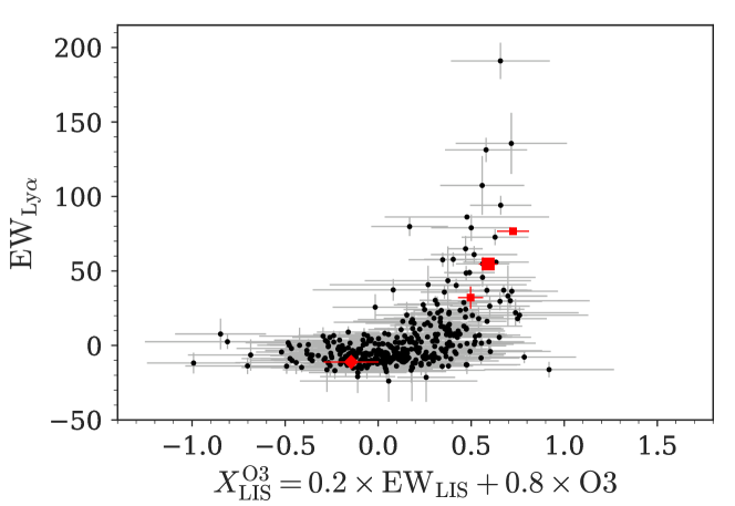
Figure 6: Ly$\alpha$ equivalent width vs. $X_{\mathrm{Ly}\alpha}$, a linear combination of O3 and EW_LIS that maximizes the Spearman rank correlation with EW_Lyα: $r_{\rm Sp}=0.49$, $p=1.5\times 10^{-24}$. Approximately half of the ordering in observed EW_Lyα is explained by these two variables alone, and 90% of the variance in $\rm EW_{\mathrm{Ly}\alpha}$ is accounted for by the combination of an exponential model and the 2D measurement uncertainties (Sec. 4.1). As in Fig. 5, red squares correspond to stacked measurements of faint $L\sim 0.1L_{*}$ Ly$\alpha$-selected galaxies from Trainor et al. (2015, 2016), and the red diamond corresponds to measurements of MS 1512-cB58 from Pettini et al. (2002) and Teplitz et al. (2000).

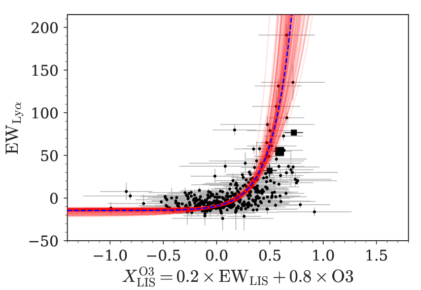
Figure 7: Data are the same as in Fig. 6, with a best-fit exponential relationship (blue dashed curve) and 100 fits to bootstap realizations of the data (faint red curves). The faint galaxy stacks and cB58 spectrum (square and diamond symbols) are not used in calculating the best-fit model parameters, but their positions are well-described by our exponential model.

4.1 Exponential Model and Variance

Motivated by the distribution of points in Fig. 6, we fit an exponential model to the data. Because there are large uncertainties in both axes, we choose model parameters to minimize the 2D distance between the model and data, scaled by the corresponding uncertainties in each dimension. In effect, we define a 2D analog of the traditional $\chi^{2}$ parameter:

$$\chi_{\mathrm{2D}}^{2} =\sum_{i}\left(\left(\frac{x_{i}-x_{c,i}}{\sigma_{x,i}}\right)^{2}+\left(\frac{y_{i}-y_{c,i}}{\sigma_{y,i}}\right)^{2}\right)$$ (13)

which our model-fitting seeks to minimize. In the above equation, $x_{i}$ and $y_{i}$ represent the values of $\rm EW_{\mathrm{Ly}\alpha}$ and $X_{\mathrm{LIS}}^{\mathrm{O3}}$ for the $i^{\mathrm{th}}$ object in our sample; $\sigma_{x,i}$ and $\sigma_{y,i}$ are the associated uncertainties for that object; and $(x_{c,i},\,y_{c,i})$ is the closest point on the model curve to the observed values $x_{i}$ and $y_{i}$, scaled by their corresponding uncertainties. Our model takes the following form:

$$\rm EW_{\mathrm{Ly}\alpha} =\mathrm{EW}_{0}+A\,\mathrm{e}^{X_{\mathrm{LIS}}^{\mathrm{O3}}/\beta}$$ (14)

where the best fit coefficients and 1D marginalized uncertainties are found to be:

$$\mathrm{EW}_{0} =-15\pm 2$$ (15)

$$A =5\pm 2$$ (16)

$$\beta =0.19\pm 0.04$$ (17)

The uncertainties in the model parameters are calculated by repeating the fit on 500 bootstrap samples of the data, where each bootstrap sample contains 377 points and their corresponding uncertainties selected at random (with replacement) from the true set of 377 points in the sample. Fig. 7 displays the best fit curve along with 100 representative fits to the bootstrap samples to demonstrate the uncertainty in the fit model.

The best-fit curve corresponds to $\chi_{\mathrm{2D}}^{2}=515$ for 377 observations, or $\chi_{\mathrm{2D}}^{2}/N_{\mathrm{dof}}=1.36$. Being above unity, this value indicates that the typical observations differ from the best-fit model by more than their formal uncertainties, such that there is intrinsic scatter in the relationship between $\rm EW_{\mathrm{Ly}\alpha}$ and $X_{\mathrm{LIS}}^{\mathrm{O3}}$ that is neither described by our model nor by our estimated observational uncertainties.

In order to determine the fraction of the total variance in $\rm EW_{\mathrm{Ly}\alpha}$ captured by the combination of our model and our measurment uncertainties, we perform the following exercise. We begin by assigning each object a fiducial value of $\rm EW_{\mathrm{Ly}\alpha}$ and $X_{\mathrm{LIS}}^{\mathrm{O3}}$ according to the nearest point to the observed values on the best-fit curve (where proximity to the curve is calculated in 2D, weighted by the uncertainty in each dimension). Each point is then perturbed in both dimensions, with the perturbation drawn from a gaussian distribution $\phi(\mu,\sigma)$ with $\mu=0$ and $\sigma$ equal to the estimated uncertainty in $\rm EW_{\mathrm{Ly}\alpha}$ or $X_{\mathrm{LIS}}^{\mathrm{O3}}$ for that object. The resulting simulated data thus represents a hypothetical sample consistent with the model, with scatter given only by the observational uncertainties.

A new fit to the resulting simulated data set is calculated (i.e., new coefficients are calculated for Eqs. 15$-$17), and the following statistics are calculated to assess the variance in the simulated data: (1) the Spearman rank correlation coefficient $r_{s}$ of the simulated data, and (2) the $\chi_{\mathrm{2D}}^{2}$ coefficient assessing the goodness of fit of the simulated data to its own best-fit model. Repeating this process 100 times, we find that the resulting distribution of statistics have $\langle r_{s}\rangle=0.59\pm 0.02$ and $\langle\chi_{\mathrm{2D}}^{2}/N_{\text{dof}}\rangle=0.98\pm 0.04$. Comparing these values to the same statistics for the real data ($r_{s}=0.49$, $\chi_{\mathrm{2D}}^{2}/N_{\text{dof}}=1.36$), we see that the simulated data have a tighter correlation and closer agreement with the fitted relation than do our real data; again, this indicates that the real data have additional sources of intrinsic scatter not described by our model or our estimated measurement errors.

We therefore model the intrinsic scatter in the relationship of $\rm EW_{\mathrm{Ly}\alpha}$ and $X_{\mathrm{LIS}}^{\mathrm{O3}}$ by assuming an underlying equation of the following form:

$$\rm EW_{\mathrm{Ly}\alpha} =f(X_{\mathrm{LIS}}^{\mathrm{O3}})+\phi(0,\sigma_{\mathrm{int}})$$ (18)

where $\phi(\mu,\sigma)$ is a number drawn from the gaussian distribution with $\mu=0$, and $\sigma_{\mathrm{int}}$ describes the intrinsic scatter in $\rm EW_{\mathrm{Ly}\alpha}$ at fixed $X_{\mathrm{LIS}}^{\mathrm{O3}}$. In this manner, we can simulate values of $\rm EW_{\mathrm{Ly}\alpha}$ and $X_{\mathrm{LIS}}^{\mathrm{O3}}$ drawn from the model distribution (including random perturbations corresponding to the estimated measurements uncertainties, as above), but with an additional term corresponding to the assumed intrinsic scatter that can be increased until the simulated data have similar total scatter (parameterized by $r_{s}$ and $\chi_{\mathrm{2D}}^{2}$) to the observed data.

In practice, we find that a value $\sigma_{\mathrm{int}}=7\pm 1\,\textrm{\AA}$ produces the best match to the statistical properties of the observed data, with $r_{s}=0.50\pm 0.03$ and $\chi_{\mathrm{2D}}^{2}/N_{\text{dof}}=1.33\pm 0.06$. Adopting this value for $\sigma_{\mathrm{int}}$ implies that the intrinsic variance in $\rm EW_{\mathrm{Ly}\alpha}$ not described by our model is $\sigma_{\mathrm{int}}^{2}=50\,\textrm{\AA}^{2}$, while the total variance in $\rm EW_{\mathrm{Ly}\alpha}$ in our data set is $\sigma_{\mathrm{obs}}^{2}=512\,\textrm{\AA}^{2}$. Assuming we have $\sigma_{\mathrm{obs}}^{2}=\sigma_{\mathrm{mod}}^{2}+\sigma_{\mathrm{int}}^{2}+\sigma_{\mathrm{meas}}^{2}$, we find that $\sim$90% of the total variance in $\rm EW_{\mathrm{Ly}\alpha}$ is accounted for by our exponential model and the estimated measurement errors.

The apparent success of our two-parameter model for predicting $\rm EW_{\mathrm{Ly}\alpha}$ deserves some inspection, particularly in light of the well-known tendency (described in Sec. 1 and below) for Ly$\alpha$ emission to display substantial scatter with respect to galaxy properties. We address this topic in Sec. 6.

5 Conditional Probabilities for Ly$\alpha$ Detection

Despite the apparent success of the model above in self-consistently describing the behavior of $\rm EW_{\mathrm{Ly}\alpha}$, it has several shortcomings. Specifically, the model described above allows us to predict the net Ly$\alpha$ emission of a given galaxy based on measurements of $\rm EW_{\mathrm{LIS}}$ and O3, but Figs. 6$-$7 reveal substantial observational scatter in this relation that is not described by our exponential model. Furthermore, it is not obvious that an exponential model is physically meaningful for describing the dependence of Ly$\alpha$ emission on these properties.

An alternative method of describing the dependence of Ly$\alpha$ emission on galaxy properties would be to relinquish analytical functions for $\rm EW_{\mathrm{Ly}\alpha}$ in favor of a non-parametric model for the conditional probability of detecting Ly$\alpha$, given a value for one or more other galaxy parameters. While this method does not provide an expected numerical value for $\rm EW_{\mathrm{Ly}\alpha}$, it allows us to explicitly describe how the detection fraction (as well as the stochasiticity in observed Ly$\alpha$ emission) varies as a function of galaxy properties.

5.1 Methodology

For the majority of the empirical parameters listed in Table 1, we construct conditional probability functions in two ways. First, we bin the full set of galaxies for which each indicator is measured into bins with widths that are allowed to vary in order to contain at least 30 galaxies per bin. Within each bin, the fraction of galaxies with detected Ly$\alpha$ in net emission ($\rm EW_{\mathrm{Ly}\alpha}>0$) is plotted as a yellow bar in the corresponding panel of Figs. 8$-$9; the fraction of galaxies that are net Ly$\alpha$ absorbers ($\rm EW_{\mathrm{Ly}\alpha}\leq 0$) is plotted as a blue bar in the negative direction. This empirical Ly$\alpha$-emitter fraction as a function of an observed parameter $X$ can be interpreted as the conditional probability distribution $P($$\rm EW_{\mathrm{Ly}\alpha}$ $>0\,|\,X)$, hereafter $P_{\mathrm{em}}^{\mathrm{Ly}\alpha}(X)$.

Displaying the empirical Ly$\alpha$-emitter fraction in this way has the useful property that every galaxy contributes to the number of absorbers or emitters for a single bin, which means that each bin is independent. However, assigning each galaxy to a specific bin based on the observed value of a given Ly$\alpha$-predicting parameter neglects the fact that the parameter values that define the horizontal axes of Figs. 8$-$9 have their own observational uncertainties, which inhibits their assignment to a single specific bin. Likewise, the observational uncertainty on $\rm EW_{\mathrm{Ly}\alpha}$ prevents a clean separation between observed Ly$\alpha$-emitters and absorbers. For this reason, we construct a second, unbinned estimator of $P_{\mathrm{em}}^{\mathrm{Ly}\alpha}(X)$ that explicitly incorporates both of these uncertainties.

Our unbinned estimator of $P_{\mathrm{em}}^{\mathrm{Ly}\alpha}(X)$ represents each galaxy observation as a pair of 1D gaussian probability distributions of the form $\phi(X\,|\,\mu=X_{i},\sigma=\sigma_{X,i})$, where $X_{i}$ and $\sigma_{X,i}$ are the observed value and observational uncertainty on parameter $X$ for galaxy $i$. Two distributions of this form are generated for each galaxy, with one distribution being normalized by the probability of the observed galaxy being a Ly$\alpha$ emitter, and the second normalized by the probability of being an absorber. Formally, we calculate the probability of an observed galaxy being a Ly$\alpha$ emitter from the measured value of $\rm EW_{\mathrm{Ly}\alpha}$ and its corresponding uncertainty $\sigma_{\mathrm{EW,Ly}\alpha}$:

$$P_{\mathrm{em},i} =\frac{1}{2}\mathrm{erf}\left(\frac{\mathrm{EW}_{\mathrm{Ly}\alpha,i}}{\sqrt{2}\,\sigma_{\mathrm{EW,Ly}\alpha,i}}\right)+\frac{1}{2}$$ (19)

$$P_{\mathrm{abs},i} =1-P_{\mathrm{em},i}$$ (20)

Thus, a galaxy with $\rm EW_{\mathrm{Ly}\alpha}$ $>0$ and $\rm EW_{\mathrm{Ly}\alpha}$ $\gg\sigma_{\mathrm{EW,Ly}\alpha}$ will have $P_{\mathrm{em}}\approx 1$ and $P_{\mathrm{abs}}\approx 0$; the “emitter” and “absorber” gaussian probability distributions are then normalized such that their integrals equal $P_{\mathrm{em}}$ and $P_{\mathrm{abs}}$, respectively. The inferred incidence $\eta$ of Ly$\alpha$ emitters (absorbers) in our sample is then the sum of all the emitter (absorber) distributions:

$$\eta_{\mathrm{em}}(X) =\sum_{i}P_{\mathrm{em},i}\,\phi(X\,|\,X_{i},\sigma_{X,i})$$ (21)

$$\eta_{\mathrm{abs}}(X) =\sum_{i}P_{\mathrm{abs},i}\,\phi(X\,|\,X_{i},\sigma_{X,i})$$ (22)

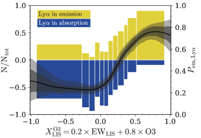
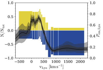
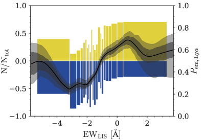
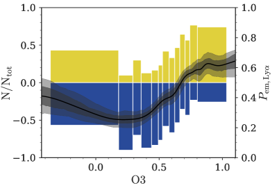
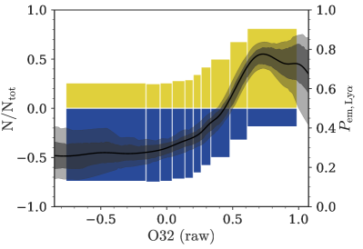
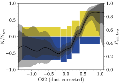
Figure 8: Conditional probability distributions for detecting Ly$\alpha$ in net emission (i.e., with $\rm EW_{\mathrm{Ly}\alpha}>0$) as a function of other galaxy parameters. Yellow (blue) bars represent the fraction of Ly$\alpha$ emitters (absorbers) found within a given bin as shown by the left-hand vertical axis. Bins sizes and boundaries are determined in order to ensure at least 30 objects are included per bin while allowing the number of bins to vary. Black lines indicate the conditional probability of Ly$\alpha$ detection (according to the right-hand vertical axis) at a given value of the parameter shown on the horizontal axis. Dark (light) gray shaded regions indicate the 68% (95%) confidence intervals on this conditional probability. Curves are determined based on the unbinned, non-parametric model described in Sec. 5.1, which depends on the measured parameter values and their uncertainties. $P_{\mathrm{em}}^{\mathrm{Ly}\alpha}$ represents $P($$\rm EW_{\mathrm{Ly}\alpha}$ $>0\,|\,X)$, where $X$ is the parameter given on the horizontal axis. The parameters displayed here are all relatively effective predictors of Ly$\alpha$ emission, with $X_{\mathrm{LIS}}^{\mathrm{O3}}$ and O32 being particularly effective.

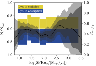
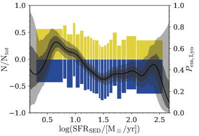
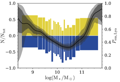
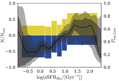
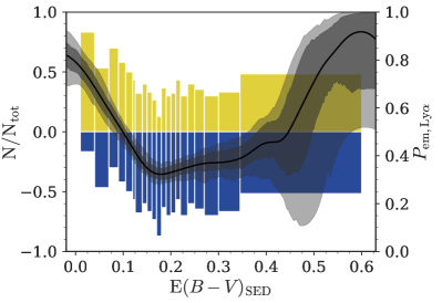
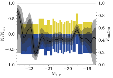
Figure 9: Continuation of Fig. 8. Conditional probability distributions for the probability of Ly$\alpha$ detection as a function of SFR, SED-fit parameters, and other photometric galaxy parameters. The parameters in this figure are all relatively weak predictors of $\rm EW_{\mathrm{Ly}\alpha}$ compared to the parameters displayed in Fig. 8; measuring the value of one of these parameters does not generally provide a strong prior on the probability of detecting Ly$\alpha$ in emission.

A galaxy that is a clear Ly$\alpha$ emitter ($P_{\mathrm{em}}\approx 1$) will therefore increase the integral of $\eta_{\mathrm{em}}$ by one over the distribution of $X$. This contribution to the incidence will be localized to a specific value of $X$ if $\sigma_{X,i}$ is small, whereas the contribution to the total incidence will be spread across a large fraction of the distribution if $\sigma_{X,i}$ is large. Finally, the inferred probability of Ly$\alpha$ emission given the observation of a galaxy with measured parameter value $X$ is taken to be the inferred incidence of Ly$\alpha$ emitters divided by the total incidence of emitters:

$$P_{\mathrm{em}}^{\mathrm{Ly}\alpha}(X) =\frac{\eta_{\mathrm{em}}(X)}{\eta_{\mathrm{em}}(X)+\eta_{\mathrm{abs}}(X)}\,\,.$$ (23)

This conditional probability is displayed as a black curve in each panel of Figs. 8$-$9. Confidence intervals for this curve are calculated by repeating the process above for 100 bootstrap realizations of the data and identifying the central 68% and 95% intervals; these are shown as gray shaded regions in Figs. 8$-$9.

5.2 Analysis of conditional probability distributions

The conditional probability distributions displayed in Figs. 8$-$9 reinforce the relationships between $\rm EW_{\mathrm{Ly}\alpha}$ and other galaxy properties shown in Table 1. Net Ly$\alpha$ emission is strongly associated with weak LIS absorption ($\rm EW_{\mathrm{LIS}}$ $\gtrsim-1$) and high ionization/excitation ($\mathrm{O3}\gtrsim 0.7$; $\mathrm{O32}\gtrsim 0.5$). In particular, our $X_{\mathrm{LIS}}^{\mathrm{O3}}$ metric is able to more clearly discriminate between Ly$\alpha$ emitters and absorbers than either $\rm EW_{\mathrm{LIS}}$ or O3 alone; even the most extreme values of these latter metrics only predict $\rm EW_{\mathrm{Ly}\alpha}$ $>0$ with $\sim$60% probability, whereas the highest values of $X_{\mathrm{LIS}}^{\mathrm{O3}}$ predict Ly$\alpha$ in net emission in $\sim$80% of cases. Likewise, $\lesssim$25% of galaxies with $X_{\mathrm{LIS}}^{\mathrm{O3}}<0$ display Ly$\alpha$ in net emission.

The distribution for $v_{\mathrm{Ly}\alpha}$ is also shown in Fig. 8, which demonstrates the strong dependence of $P_{\mathrm{em}}^{\mathrm{Ly}\alpha}$ on $v_{\mathrm{Ly}\alpha}$ over the range $0\lesssim v_{\mathrm{Ly}\alpha}\lesssim 800\,\textrm{km}\,\textrm{s}^{-1}$ and very low probability of Ly$\alpha$ emission for galaxies with $v_{\mathrm{Ly}\alpha}\gtrsim 800\,\textrm{km}\,\textrm{s}^{-1}$ ($P_{\mathrm{em}}^{\mathrm{Ly}\alpha}\approx 0.1-0.2$). $P_{\mathrm{em}}^{\mathrm{Ly}\alpha}$ peaks for $v_{\mathrm{Ly}\alpha}\approx 0$, consistent with the model described in Secs. 1 & 3.2.1.

Other than $v_{\mathrm{Ly}\alpha}$, O32 is again the most direct predictor of net Ly$\alpha$ emission or absorption: even the dust-uncorrected (i.e., raw) values are approximately as effective at predicting $\rm EW_{\mathrm{Ly}\alpha}$ $>0$ as $X_{\mathrm{LIS}}^{\mathrm{O3}}$, and the dust-corrected measurements predict Ly$\alpha$ emission with $>$80% probability at the highest O32 values and $\lesssim$20% at the lowest values. As discussed in Secs. 3.3.2$-$3.3.3, this strong correlation may be due in part to the fact that dust-corrected O32 is a quite direct measure of the ionization parameter in ionization-bounded nebulae, but it may also be due to the fact that elevated O32 may indicate density-bounded nebulae that facilitate Ly$\alpha$ escape as well as production. Nonetheless, an observer who merely wishes to predict the net Ly$\alpha$ emission of a galaxy (remaining agnostic to the circumstances that facilitate this emission) will find O32 to be an effective indicator of this emission. However, the caveat to the effectiveness of this indicator remains the observational difficulty of obtaining high-S/N measurements of the [O III] and [O II] emission lines (the latter of which can be extremely faint in the high-ionization galaxies typical at high-$z$) as well as the Balmer lines necessary to correct for differential attenuation by dust. This effect is seen in the small number of bins (which must each contain 30$+$ galaxies) in each of the O32 plots, as well as in the broad confidence intervals for the corresponding unbinned relations.

Note that in many of the panels of Figs. 8$-$9, the trends apparently reverse toward the extrema of a given parameter value. Given that these regions of parameter space are sparsely populated (as can be seen based on the width of the blue and yellow bars) and the confidence intervals on $P_{\mathrm{em}}^{\mathrm{Ly}\alpha}$ diverge, we interpret majority of this apparent aberrant behavior as a regression toward the overall average rate of Ly$\alpha$ emission ($P_{\mathrm{em}}^{\mathrm{Ly}\alpha}(X)\approx\langle P_{\mathrm{em}}^{\mathrm{Ly}\alpha}\rangle\approx 0.5$) when the parameter uncertainties are large. This effect is particularly noticeable in the panel for $\rm EW_{\mathrm{LIS}}$, where the highest and lowest bins appear particularly dominated by observational error – in this case, we expect that the trend between $\rm EW_{\mathrm{LIS}}$ and $\rm EW_{\mathrm{Ly}\alpha}$ is monotonically positive over the range in which both parameters are well-measured. Conversely, the relatively tight confidence intervals for $X_{\mathrm{LIS}}^{\mathrm{O3}}$ and O32 appear to indicate real flattening in their relationships with $P_{\mathrm{em}}^{\mathrm{Ly}\alpha}$; some non-negligible stochasticity in $\rm EW_{\mathrm{Ly}\alpha}$ appears to be present that is not accounted for by these factors even when they are well-measured, as demonstrated by the $\sim$20% of Ly$\alpha$ emitters (absorbers) that are present even at the lowest (highest) values of these parameters.

Fig. 9 displays the conditional probability distributions for several parameters that are only weakly correlated with $\rm EW_{\mathrm{Ly}\alpha}$, again reinforcing the results shown in Table 1. In particular, SFR_Hα and M_UV display negligible predictive power related to Ly$\alpha$ emission over the parameter space sampled by our galaxies. E$(B-V)_{\mathrm{SED}}$ is an effective predictor of $P_{\mathrm{em}}^{\mathrm{Ly}\alpha}$ at the lowest reddenings (E$(B-V)_{\mathrm{SED}}\lesssim 0.2$), but Ly$\alpha$ emitters and absorbers appear almost equally common among galaxies with higher reddening values. Surprisingly, the incidence of Ly$\alpha$ emitters appears to grow slightly with increasing E$(B-V)_{\mathrm{SED}}$ for E$(B-V)_{\mathrm{SED}}>0.2$. This effect may be dominated by the relatively uncertain values of E$(B-V)_{\mathrm{SED}}$, which is somewhat degenerate with stellar population age, causing a regression toward the population mean. $P_{\mathrm{em}}^{\mathrm{Ly}\alpha}$ shows a moderate increase as SFR_SED decreases or sSFR increases.

Stellar mass ($M_{*}$) displays perhaps the most interesting relationship with $\rm EW_{\mathrm{Ly}\alpha}$ that is not obvious from the Spearman correlation alone: Ly$\alpha$ emission probability increases significantly among both the lowest- and highest-mass galaxies. The low-mass relationship (along with the trends in SFR and sSFR) may reflect the tendency for low-mass, low-SFR galaxies to have relatively porous interstellar media and high nebular excitation (see, e.g., Trainor et al. 2015, 2016). Although galaxies with clear signatures of AGN activity were removed from our sample, the excess of Ly$\alpha$ emitters at high galaxy masses may reflect residual AGN in our sample. It is also possible that some galaxy masses in our sample are over-estimated due to strong line emission that contaminates the rest-frame optical photometry; SED-fit masses are especially sensitive to this effect at high redshift (see e.g., Schenker et al. 2013). In this case, the increase in Ly$\alpha$ emission among galaxies with large inferred stellar masses could be caused by the underlying association between Ly$\alpha$ and optical emission line strength (i.e., nebular excitation). The Ly$\alpha$-emitting behavior of high-mass galaxies will be investigated in future work.

In general, these conditional probability distributions may be used to inform analyses of the Ly$\alpha$-detection fraction of galaxies at the highest redshifts, where the opacity of the neutral IGM may suppress the observed Ly$\alpha$ emission from intrinsic Ly$\alpha$ emitters. By using other observed properties of galaxies as priors input to the distributions above, it will be possible to more accurately characterize the degree to which evolution in both IGM and galaxy properties shape the distribution of observed Ly$\alpha$ emission.

6 Comparison to Recent Work

A few recent studies in the low-redshift Universe have measured correlations between Ly$\alpha$ emission and other galaxy properties with the goal of predicting the Ly$\alpha$ emission. Hayes et al. (2014) present data from the Lyman-Alpha Reference Sample (LARS; Östlin et al. 2014), comparing Ly$\alpha$ emission with 12 different global galaxy properties derived from imaging and spectroscopy. They find significant correlations in which normalized Ly$\alpha$ emission is highest among galaxies with low SFR, low dust content (inferred by nebular line ratios or the UV slope), low mass, and nebular properties indicative of high excitation and low metallicity. The Hayes et al. (2014) study differs from the work presented here in that the their individual measurements have much higher signal-to-noise ratios (S/N) but are much fewer in number (12 galaxies in LARS vs. the 703 galaxies in this paper). Furthermore, the original LARS sample did not include rest-UV continuum spectroscopy covering the interstellar absorption lines; while these data were later collected via HST/COS spectroscopy and presented by Rivera-Thorsen et al. (2015), there is currently no simultaneous analysis of the predictive power of combined rest-UV and rest-optical spectroscopic diagnostics of Ly$\alpha$ emission in LARS.

Recent results by Yang et al. (2017) are more directly comparable to those presented here: Yang et al. (2017) analyze HST/COS spectra of 43 “green pea” galaxies at $z\sim 0.1-0.3$ with SDSS optical spectroscopy. The authors find that the escape fraction of Ly$\alpha$ is anticorrelated with the velocity width of the Ly$\alpha$ line profile, the nebular dust extinction, and the stellar mass, as well as positively correlated with the O32 ratio. Each of these relationships have Spearman rank-correlation coefficients of $r\sim 0.5-0.6$; while the contributions of observational uncertainties to this scatter are not explicitly calculated, the quoted uncertainties suggest that these contributions are neglible. Furthermore, Yang et al. (2017) fit a linear combination of the nebular extinction E($B-V$) and the velocity offset of the red Ly$\alpha$ peak, finding that the resulting relation fits the observed Ly$\alpha$ escape fraction with a 1$\sigma$ scatter of 0.3 dex. Notably, this multi-parameter relationship is similar to our own work in Sec. 4, but it differs in that both included parameters (the Ly$\alpha$ velocity offset and inferred dust extinction) fall into the category of empirical parameters we have associated with Ly$\alpha$ escape (Sec. 3.2), rather than including a proxy for the efficiency of Ly$\alpha$ production (Sec. 3.3). As with the Hayes et al. (2014) study, Yang et al. (2017) have the advantage over our own work of measuring individual spectroscopic parameters at high S/N, but they include a much smaller sample size. The Yang et al. (2017) sample also only includes galaxies selected to be spatially compact, low-mass, and high-excitation, whereas the KBSS sample includes 15$\times$ more galaxies over a much broader range of properties. Nonetheless, the different selection biases and relative advantages of low- and high-redshift galaxy samples make these $z\sim 0-0.3$ surveys (including continued HST/COS spectroscopy) an effective complement to the work presented here.

While not directly focused on predicting Ly$\alpha$ emission, recent work from the HiZELS survey (Geach et al., 2008; Sobral et al., 2009) has pointed to the complex relationships between Ly$\alpha$ and other recombination line emission. In particular, Oteo et al. (2015) demonstrate that galaxies selected on the basis of H$\alpha$ emission display only weak Ly$\alpha$ emission on average. This result is consistent with the first panel of Fig. 9 and the discussion in Sec. 3.3.1 of this paper, as we also find $L_{\mathrm{H}\alpha}$ to be a poor predictor of Ly$\alpha$ emission. Although the HiZELS galaxies do not have deep rest-UV spectra, we expect that their low Ly$\alpha$ escape fractions would be associated with strong LIS absorption, such that they may lie near cB58 in the O3-$\rm EW_{\mathrm{LIS}}$ plane displayed in Fig. 5 (i.e., the parameter space associated with high rates of intrinsic Ly$\alpha$ production, but low rates of Ly$\alpha$ escape).

In more recent work, Du et al. (2018) present a systematic study of the redshift evolution of rest-UV spectroscopic properties of galaxies over $z\approx 2-4$, including the variation of Ly$\alpha$ with other galaxy properties in this epoch. The Du et al. (2018) spectroscopic sample is also drawn from the KBSS and has substantial overlap with the galaxies presented here. Broadly, the authors find that the relationship between $\rm EW_{\mathrm{Ly}\alpha}$ and $\rm EW_{\mathrm{LIS}}$ is invariant with redshift for $2\lesssim z\lesssim 4$, with a similarly invariant (but weaker) relationship between $\rm EW_{\mathrm{Ly}\alpha}$ and E$(B-V)_{\mathrm{SED}}$. In addition to these indicators of Ly$\alpha$ escape, Du et al. (2018) argue that the association between the equivalent width of C III] and $\rm EW_{\mathrm{Ly}\alpha}$ (which they find to be similar at $z\sim 2$ and $z\sim 3$) represents the dependence of $\rm EW_{\mathrm{Ly}\alpha}$ on the instrinsic production rate of Ly$\alpha$ emission. One interesting point of comparison between their results and those presented here regards the relationship between $\rm EW_{\mathrm{Ly}\alpha}$ and M_UV; in their $z\sim 2$ galaxy bin (which is most similar to the galaxies presented here), Du et al. (2018) find no relationship between $\rm EW_{\mathrm{Ly}\alpha}$ and M_UV, but they find an increasingly strong relationship with increasing redshift. Likewise, Oyarzún et al. (2017) find a positive correlation between M_UV and $\rm EW_{\mathrm{Ly}\alpha}$, but the relationship appears to rely on the inclusion of lower-luminosity galaxies than are included in this sample (although similar to the galaxies described in Trainor et al. 2015, 2016; see Figs. 5 & 6 here) and the extension to higher redshifts. This variation may help explain the high $\rm EW_{\mathrm{Ly}\alpha}$ values seen generically in the lowest-luminosity galaxies at $z\sim 2$ (e.g., Stark et al. 2013), which are perhaps better analogs for typical galaxies at the highest redshifts than the more luminous $z\sim 2$ galaxies described in this paper.

The results of Du et al. (2018) are in general agreement with those presented here, with the exception that Du et al. (2018) limit their analysis to composite rest-UV spectra (i.e., they include no rest-optical data, nor do they analyze the spectra of individual galaxies), and they consider the redshift evolution of these trends. The Du et al. composite spectra achieve higher S/N measurements of individual features than the measurements we consider here, but they also smooth over the intrinsic object-to-object variation among galaxies – variation that we highlight in this paper, particularly in Sec. 5. Together, therefore, these two studies provide a comprehensive view of the average trends among net Ly$\alpha$ emission and the processes of production and escape, while also demonstrating the substantial stochasticity that accompanies these broader trends.

Another complementary aspect of these works is that Du et al. (2018) demonstrate that individual parameters related to Ly$\alpha$ production and escape (i.e., $\rm EW_{\mathrm{LIS}}$, E$(B-V)$, and proxies for nebular excitation) show similar relationships with $\rm EW_{\mathrm{Ly}\alpha}$ across $2<z<4$, despite the fact that the ubiquity of $\rm EW_{\mathrm{Ly}\alpha}$ emission itself (and its dependence on M_UV, SFR, and $M_{*}$) evolves significantly over this period. This invariance suggests that the models for Ly$\alpha$ emission developed here – particularly those shown in Figs. 6 & 8 – may be expected to remain useful even at higher redshifts where the intrinsic Ly$\alpha$ emission of galaxies is more difficult to directly measure.

7 Conclusions

We have presented an empirical analysis of factors affecting Ly$\alpha$ production and escape in a sample of 703 star-forming galaxies from the Keck Baryonic Structure Survey at $z\approx 1.5-3.5$. Our primary indicators of Ly$\alpha$ escape efficiency include the velocity offset of the Ly$\alpha$ line and the equivalent width in absorption of low-ionization interstellar lines, $\rm EW_{\mathrm{LIS}}$, and we find that these proxies for Ly$\alpha$ escape are strongly associated with the directly-measured Ly$\alpha$ escape fraction, $f_{\mathrm{esc}}$. Our indicators of Ly$\alpha$ production include the O3 and O32 ratios, which we argue are effective diagnostics of the ionization conditions within the H II regions from which Ly$\alpha$ photons originate. Several other galaxy parameters including stellar mass, star-formation rate, luminosity, and reddenning are shown to have much weaker relationships with observed Ly$\alpha$ emission.

We propose that $\rm EW_{\mathrm{LIS}}$ and O3 are the most useful predictors of $\rm EW_{\mathrm{Ly}\alpha}$ because of their potential for observability in cases when the Ly$\alpha$ line is not directly detectable (or may be strongly affected by IGM absorption) and because of their strong individual correlations with $\rm EW_{\mathrm{Ly}\alpha}$ and lack of correlation with each other. We then construct a new quantity, $X_{\mathrm{LIS}}^{\mathrm{O3}}$, which is a linear combination of $\rm EW_{\mathrm{LIS}}$ and O3 with coefficients chosen to maximize the association between $X_{\mathrm{LIS}}^{\mathrm{O3}}$ and $\rm EW_{\mathrm{Ly}\alpha}$.

We find that the combination of O3 and $\rm EW_{\mathrm{LIS}}$ predicts net $\rm EW_{\mathrm{Ly}\alpha}$ with less scatter than any single variable captured by our survey that does not require measurement of the Ly$\alpha$ line; $\sim$50% of the ordering in observed $\rm EW_{\mathrm{Ly}\alpha}$ is captured by $X_{\mathrm{LIS}}^{\mathrm{O3}}$. After accounting for measurement uncertainties and fitting an exponential model for $\rm EW_{\mathrm{Ly}\alpha}$ as a function of $X_{\mathrm{LIS}}^{\mathrm{O3}}$, we estimate that the combination of our model and observational error account for 90% of the total variance in $\rm EW_{\mathrm{Ly}\alpha}$ at fixed $X_{\mathrm{LIS}}^{\mathrm{O3}}$.

We also estimate the conditional probability of detecting net Ly$\alpha$ emission or absorption in slit spectroscopy of a galaxy as a function of various galaxy parameters. We find that galaxies with $X_{\mathrm{LIS}}^{\mathrm{O3}}>0.6$ have an 80% probability of being net Ly$\alpha$ emitters, while those with $X_{\mathrm{LIS}}^{\mathrm{O3}}<0$ have less than a 25% probability of exhibiting net emission. Similarly strong variation in the probability of net Ly$\alpha$ emission is seen when adopting a prior based on O32, while constraints on photometric or SED-fit parameters or H$\alpha$-based SFR have negligible utility as priors over the parameter space probed by our sample.

Given the many factors affecting net Ly$\alpha$ emission, our two-parameter model for $X_{\mathrm{LIS}}^{\mathrm{O3}}$ is remarkably successful at describing the variation in Ly$\alpha$ emission across a large, heterogenous set of star-forming galaxies. We suggest that this success indicates that the wide variety of processes affecting Ly$\alpha$ emission can be broadly categorized as relating to Ly$\alpha$ production or escape, and capturing these two different “meta-parameters” is an essential component of any model for Ly$\alpha$ emission from galaxies.

References

- Astropy Collaboration et al. (2013) Astropy Collaboration, Robitaille, T. P., Tollerud, E. J., Greenfield, P., Droettboom, M., Bray, E., Aldcroft, T., Davis, M., Ginsburg, A., & Price-Whelan, A. M. 2013, A&A, 558, A33
- Atek et al. (2009) Atek, H., Kunth, D., Schaerer, D., Hayes, M., Deharveng, J. M., Östlin, G., & Mas-Hesse, J. M. 2009, A&A, 506, L1
- Atek et al. (2010) Atek, H., Malkan, M., McCarthy, P., Teplitz, H. I., Scarlata, C., Siana, B., Henry, A., Colbert, J. W., Ross, N. R., Bridge, C., Bunker, A. J., Dressler, A., Fosbury, R. A. E., Martin, C., & Shim, H. 2010, ApJ, 723, 104
- Bacon et al. (2015) Bacon, R., Brinchmann, J., Richard, J., Contini, T., Drake, A., Franx, M., Tacchella, S., Vernet, J., Wisotzki, L., Blaizot, J., Bouché, N., Bouwens, R., Cantalupo, S., Carollo, C. M., Carton, D., Caruana, J., Clément, B., Dreizler, S., Epinat, B., Guiderdoni, B., Herenz, C., Husser, T.-O., Kamann, S., Kerutt, J., Kollatschny, W., Krajnovic, D., Lilly, S., Martinsson, T., Michel-Dansac, L., Patricio, V., Schaye, J., Shirazi, M., Soto, K., Soucail, G., Steinmetz, M., Urrutia, T., Weilbacher, P., & de Zeeuw, T. 2015, A&A, 575, A75
- Baldwin et al. (1981) Baldwin, J. A., Phillips, M. M., & Terlevich, R. 1981, PASP, 93, 5
- Borthakur et al. (2014) Borthakur, S., Heckman, T. M., Leitherer, C., & Overzier, R. A. 2014, Science, 346, 216
- Brammer et al. (2012) Brammer, G. B., van Dokkum, P. G., Franx, M., Fumagalli, M., Patel, S., Rix, H.-W., Skelton, R. E., Kriek, M., Nelson, E., Schmidt, K. B., Bezanson, R., da Cunha, E., Erb, D. K., Fan, X., Förster Schreiber, N., Illingworth, G. D., Labbé, I., Leja, J., Lundgren, B., Magee, D., Marchesini, D., McCarthy, P., Momcheva, I., Muzzin, A., Quadri, R., Steidel, C. C., Tal, T., Wake, D., Whitaker, K. E., & Williams, A. 2012, ApJS, 200, 13
- Bruzual & Charlot (2003) Bruzual, G. & Charlot, S. 2003, MNRAS, 344, 1000
- Calzetti et al. (2000) Calzetti, D., Armus, L., Bohlin, R. C., Kinney, A. L., Koornneef, J., & Storchi-Bergmann, T. 2000, ApJ, 533, 682
- Cantalupo et al. (2014) Cantalupo, S., Arrigoni-Battaia, F., Prochaska, J. X., Hennawi, J. F., & Madau, P. 2014, Nature, 506, 63
- Cantalupo et al. (2012) Cantalupo, S., Lilly, S. J., & Haehnelt, M. G. 2012, MNRAS, 425, 1992
- Cantalupo et al. (2005) Cantalupo, S., Porciani, C., Lilly, S. J., & Miniati, F. 2005, ApJ, 628, 61
- Cardelli et al. (1989) Cardelli, J. A., Clayton, G. C., & Mathis, J. S. 1989, ApJ, 345, 245
- Chabrier (2003) Chabrier, G. 2003, PASP, 115, 763
- Cowie & Hu (1998) Cowie, L. L. & Hu, E. M. 1998, AJ, 115, 1319
- de Barros et al. (2016) de Barros, S., Vanzella, E., Amorín, R., Castellano, M., Siana, B., Grazian, A., Suh, H., Balestra, I., Vignali, C., Verhamme, A., Zamorani, G., Mignoli, M., Hasinger, G., Comastri, A., Pentericci, L., Pérez-Montero, E., Fontana, A., Giavalisco, M., & Gilli, R. 2016, A&A, 585, A51
- Dopita & Sutherland (2003) Dopita, M. A. & Sutherland, R. S. 2003, Astrophysics of the diffuse universe, Berlin, New York: Springer, 2003. Astronomy and astrophysics library, ISBN 3540433627
- Du et al. (2018) Du, X., Shapley, A. E., Reddy, N. A., Jones, T., Stark, D. P., Steidel, C. C., Strom, A. L., Rudie, G. C., Erb, D. K., Ellis, R. S., & Pettini, M. 2018, ApJ, 860, 75
- Erb et al. (2016) Erb, D. K., Pettini, M., Steidel, C. C., Strom, A. L., Rudie, G. C., Trainor, R. F., Shapley, A. E., & Reddy, N. A. 2016, ApJ, 830, 52
- Erb et al. (2014) Erb, D. K., Steidel, C. C., Trainor, R. F., Bogosavljević, M., Shapley, A. E., Nestor, D. B., Kulas, K. R., Law, D. R., Strom, A. L., Rudie, G. C., Reddy, N. A., Pettini, M., Konidaris, N. P., Mace, G., Matthews, K., & McLean, I. S. 2014, ApJ, 795, 33
- Finkelstein et al. (2011) Finkelstein, S. L., Hill, G. J., Gebhardt, K., Adams, J., Blanc, G. A., Papovich, C., Ciardullo, R., Drory, N., Gawiser, E., Gronwall, C., Schneider, D. P., & Tran, K.-V. 2011, ApJ, 729, 140
- Fletcher et al. (2018) Fletcher, T. J., Robertson, B. E., Nakajima, K., Ellis, R. S., Stark, D. P., & Inoue, A. 2018, ArXiv e-prints
- Geach et al. (2008) Geach, J. E., Smail, I., Best, P. N., Kurk, J., Casali, M., Ivison, R. J., & Coppin, K. 2008, MNRAS, 388, 1473
- Hagen et al. (2016) Hagen, A., Zeimann, G. R., Behrens, C., Ciardullo, R., Grasshorn Gebhardt, H. S., Gronwall, C., Bridge, J. S., Fox, D. B., Schneider, D. P., Trump, J. R., Blanc, G. A., Chiang, Y.-K., Chonis, T. S., Finkelstein, S. L., Hill, G. J., Jogee, S., & Gawiser, E. 2016, ApJ, 817, 79
- Hayes et al. (2014) Hayes, M., Östlin, G., Duval, F., Sandberg, A., Guaita, L., Melinder, J., Adamo, A., Schaerer, D., Verhamme, A., Orlitová, I., Mas-Hesse, J. M., Cannon, J. M., Atek, H., Kunth, D., Laursen, P., Otí-Floranes, H., Pardy, S., Rivera-Thorsen, T., & Herenz, E. C. 2014, ApJ, 782, 6
- Hayes et al. (2010) Hayes, M., Östlin, G., Schaerer, D., Mas-Hesse, J. M., Leitherer, C., Atek, H., Kunth, D., Verhamme, A., de Barros, S., & Melinder, J. 2010, Nature, 464, 562
- Henry et al. (2015) Henry, A., Scarlata, C., Martin, C. L., & Erb, D. 2015, ApJ, 809, 19
- Hoag et al. (2019) Hoag, A., Bradač, M., Huang, K., Mason, C., Treu, T., Schmidt, K. B., Trenti, M., Strait, V., Lemaux, B. C., Finney, E. Q., & Paddock, M. 2019, ApJ, 878, 12
- Hunter (2007) Hunter, J. D. 2007, Computing in Science and Engineering, 9, 90
- Izotov et al. (2016) Izotov, Y. I., Schaerer, D., Thuan, T. X., Worseck, G., Guseva, N. G., Orlitová, I., & Verhamme, A. 2016, MNRAS, 461, 3683
- Izotov et al. (2018) Izotov, Y. I., Worseck, G., Schaerer, D., Guseva, N. G., Thuan, T. X., Fricke, Verhamme, A., & Orlitová, I. 2018, MNRAS, 478, 4851
- Jones et al. (2012) Jones, T., Stark, D. P., & Ellis, R. S. 2012, ApJ, 751, 51
- Kennicutt (1998) Kennicutt, Jr., R. C. 1998, ARA&A, 36, 189
- Kollmeier et al. (2010) Kollmeier, J. A., Zheng, Z., Davé, R., Gould, A., Katz, N., Miralda-Escudé, J., & Weinberg, D. H. 2010, ApJ, 708, 1048
- Kunth et al. (1998) Kunth, D., Mas-Hesse, J. M., Terlevich, E., Terlevich, R., Lequeux, J., & Fall, S. M. 1998, A&A, 334, 11
- Martin et al. (2015) Martin, C. L., Dijkstra, M., Henry, A., Soto, K. T., Danforth, C. W., & Wong, J. 2015, ApJ, 803, 6
- Mason et al. (2018) Mason, C. A., Treu, T., Dijkstra, M., Mesinger, A., Trenti, M., Pentericci, L., de Barros, S., & Vanzella, E. 2018, ApJ, 856, 2
- McLean et al. (2012) McLean, I. S., Steidel, C. C., Epps, H. W., Konidaris, N., Matthews, K. Y., Adkins, S., Aliado, T., Brims, G., Canfield, J. M., Cromer, J. L., Fucik, J., Kulas, K., Mace, G., Magnone, K., Rodriguez, H., Rudie, G., Trainor, R., Wang, E., Weber, B., & Weiss, J. 2012, in Society of Photo-Optical Instrumentation Engineers (SPIE) Conference Series, Vol. 8446, Society of Photo-Optical Instrumentation Engineers (SPIE) Conference Series
- McLinden et al. (2011) McLinden, E. M., Finkelstein, S. L., Rhoads, J. E., Malhotra, S., Hibon, P., Richardson, M. L. A., Cresci, G., Quirrenbach, A., Pasquali, A., Bian, F., Fan, X., & Woodward, C. E. 2011, ApJ, 730, 136
- Momose et al. (2014) Momose, R., Ouchi, M., Nakajima, K., Ono, Y., Shibuya, T., Shimasaku, K., Yuma, S., Mori, M., & Umemura, M. 2014, MNRAS, 442, 110
- Momose et al. (2016) —. 2016, MNRAS, 457, 2318
- Nakajima et al. (2016) Nakajima, K., Ellis, R. S., Iwata, I., Inoue, A. K., Kusakabe, H., Ouchi, M., & Robertson, B. E. 2016, ApJ, 831, L9
- Nakajima et al. (2013) Nakajima, K., Ouchi, M., Shimasaku, K., Hashimoto, T., Ono, Y., & Lee, J. C. 2013, ApJ, 769, 3
- Oke et al. (1995) Oke, J. B., Cohen, J. G., Carr, M., Cromer, J., Dingizian, A., Harris, F. H., Labrecque, S., Lucinio, R., Schaal, W., Epps, H., & Miller, J. 1995, PASP, 107, 375
- Osterbrock (1989) Osterbrock, D. E. 1989, Astrophysics of gaseous nebulae and active galactic nuclei
- Östlin et al. (2014) Östlin, G., Hayes, M., Duval, F., Sandberg, A., Rivera-Thorsen, T., Marquart, T., Orlitová, I., Adamo, A., Melinder, J., Guaita, L., Atek, H., Cannon, J. M., Gruyters, P., Herenz, E. C., Kunth, D., Laursen, P., Mas-Hesse, J. M., Micheva, G., Otí-Floranes, H., Pardy, S. A., Roth, M. M., Schaerer, D., & Verhamme, A. 2014, ApJ, 797, 11
- Oteo et al. (2015) Oteo, I., Sobral, D., Ivison, R. J., Smail, I., Best, P. N., Cepa, J., & Pérez-García, A. M. 2015, MNRAS, 452, 2018
- Ouchi et al. (2018) Ouchi, M., Harikane, Y., Shibuya, T., Shimasaku, K., Taniguchi, Y., Konno, A., Kobayashi, M., Kajisawa, M., Nagao, T., Ono, Y., Inoue, A. K., Umemura, M., Mori, M., Hasegawa, K., Higuchi, R., Komiyama, Y., Matsuda, Y., Nakajima, K., Saito, T., & Wang, S.-Y. 2018, PASJ, 70, S13
- Oyarzún et al. (2017) Oyarzún, G. A., Blanc, G. A., González, V., Mateo, M., & Bailey, John I., I. 2017, ApJ, 843, 133
- Oyarzún et al. (2016) Oyarzún, G. A., Blanc, G. A., González, V., Mateo, M., Bailey, III, J. I., Finkelstein, S. L., Lira, P., Crane, J. D., & Olszewski, E. W. 2016, ApJ, 821, L14
- Pellegrini et al. (2012) Pellegrini, E. W., Oey, M. S., Winkler, P. F., Points, S. D., Smith, R. C., Jaskot, A. E., & Zastrow, J. 2012, ApJ, 755, 40
- Pentericci et al. (2011) Pentericci, L., Fontana, A., Vanzella, E., Castellano, M., Grazian, A., Dijkstra, M., Boutsia, K., Cristiani, S., Dickinson, M., Giallongo, E., Giavalisco, M., Maiolino, R., Moorwood, A., Paris, D., & Santini, P. 2011, ApJ, 743, 132
- Pentericci et al. (2018) Pentericci, L., Vanzella, E., Castellano, M., Fontana, A., De Barros, S., Grazian, A., Marchi, F., Bradac, M., Conselice, C. J., Cristiani, S., Dickinson, M., Finkelstein, S. L., Giallongo, E., Guaita, L., Koekemoer, A. M., Maiolino, R., Santini, P., & Tilvi, V. 2018, A&A, 619, A147
- Pettini et al. (2002) Pettini, M., Rix, S. A., Steidel, C. C., Adelberger, K. L., Hunt, M. P., & Shapley, A. E. 2002, ApJ, 569, 742
- Pettini et al. (2000) Pettini, M., Steidel, C. C., Adelberger, K. L., Dickinson, M., & Giavalisco, M. 2000, ApJ, 528, 96
- Rakic et al. (2012) Rakic, O., Schaye, J., Steidel, C. C., & Rudie, G. C. 2012, ApJ, 751, 94
- Reddy et al. (2012) Reddy, N. A., Pettini, M., Steidel, C. C., Shapley, A. E., Erb, D. K., & Law, D. R. 2012, ApJ, 754, 25
- Reddy et al. (2008) Reddy, N. A., Steidel, C. C., Pettini, M., Adelberger, K. L., Shapley, A. E., Erb, D. K., & Dickinson, M. 2008, ApJS, 175, 48
- Rhoads et al. (2000) Rhoads, J. E., Malhotra, S., Dey, A., Stern, D., Spinrad, H., & Jannuzi, B. T. 2000, ApJ, 545, L85
- Rivera-Thorsen et al. (2015) Rivera-Thorsen, T. E., Hayes, M., Östlin, G., Duval, F., Orlitová, I., Verhamme, A., Mas-Hesse, J. M., Schaerer, D., Cannon, J. M., Otí-Floranes, H., Sandberg, A., Guaita, L., Adamo, A., Atek, H., Herenz, E. C., Kunth, D., Laursen, P., & Melinder, J. 2015, ApJ, 805, 14
- Roberts-Borsani et al. (2016) Roberts-Borsani, G. W., Bouwens, R. J., Oesch, P. A., Labbe, I., Smit, R., Illingworth, G. D., van Dokkum, P., Holden, B., Gonzalez, V., Stefanon, M., Holwerda, B., & Wilkins, S. 2016, ApJ, 823, 143
- Robertson et al. (2015) Robertson, B. E., Ellis, R. S., Furlanetto, S. R., & Dunlop, J. S. 2015, ApJ, 802, L19
- Rousseeuw & Croux (1993) Rousseeuw, P. J. & Croux, C. 1993, Journal of the American Statistical Association, 88, 1273
- Rudie et al. (2012) Rudie, G. C., Steidel, C. C., Trainor, R. F., Rakic, O., Bogosavljević, M., Pettini, M., Reddy, N., Shapley, A. E., Erb, D. K., & Law, D. R. 2012, ApJ, 750, 67
- Sanders et al. (2016) Sanders, R. L., Shapley, A. E., Kriek, M., Reddy, N. A., Freeman, W. R., Coil, A. L., Siana, B., Mobasher, B., Shivaei, I., Price, S. H., & de Groot, L. 2016, ApJ, 816, 23
- Schenker et al. (2013) Schenker, M. A., Ellis, R. S., Konidaris, N. P., & Stark, D. P. 2013, ApJ, 777, 67
- Schenker et al. (2012) Schenker, M. A., Stark, D. P., Ellis, R. S., Robertson, B. E., Dunlop, J. S., McLure, R. J., Kneib, J.-P., & Richard, J. 2012, ApJ, 744, 179
- Shapley et al. (2003) Shapley, A. E., Steidel, C. C., Pettini, M., & Adelberger, K. L. 2003, ApJ, 588, 65
- Shapley et al. (2016) Shapley, A. E., Steidel, C. C., Strom, A. L., Bogosavljević, M., Reddy, N. A., Siana, B., Mostardi, R. E., & Rudie, G. C. 2016, ApJ, 826, L24
- Siana et al. (2008) Siana, B., Teplitz, H. I., Chary, R.-R., Colbert, J., & Frayer, D. T. 2008, ApJ, 689, 59
- Sobral et al. (2009) Sobral, D., Best, P. N., Geach, J. E., Smail, I., Kurk, J., Cirasuolo, M., Casali, M., Ivison, R. J., Coppin, K., & Dalton, G. B. 2009, MNRAS, 398, 75
- Song et al. (2014) Song, M., Finkelstein, S. L., Gebhardt, K., Hill, G. J., Drory, N., Ashby, M. L. N., Blanc, G. A., Bridge, J., Chonis, T., Ciardullo, R., Fabricius, M., Fazio, G. G., Gawiser, E., Gronwall, C., Hagen, A., Huang, J.-S., Jogee, S., Livermore, R., Salmon, B., Schneider, D. P., Willner, S. P., & Zeimann, G. R. 2014, ApJ, 791, 3
- Stark et al. (2017) Stark, D. P., Ellis, R. S., Charlot, S., Chevallard, J., Tang, M., Belli, S., Zitrin, A., Mainali, R., Gutkin, J., Vidal-García, A., Bouwens, R., & Oesch, P. 2017, MNRAS, 464, 469
- Stark et al. (2010) Stark, D. P., Ellis, R. S., Chiu, K., Ouchi, M., & Bunker, A. 2010, MNRAS, 408, 1628
- Stark et al. (2013) Stark, D. P., Schenker, M. A., Ellis, R., Robertson, B., McLure, R., & Dunlop, J. 2013, ApJ, 763, 129
- Steidel et al. (2000) Steidel, C. C., Adelberger, K. L., Shapley, A. E., Pettini, M., Dickinson, M., & Giavalisco, M. 2000, ApJ, 532, 170
- Steidel et al. (2003) —. 2003, ApJ, 592, 728
- Steidel et al. (2011) Steidel, C. C., Bogosavljević, M., Shapley, A. E., Kollmeier, J. A., Reddy, N. A., Erb, D. K., & Pettini, M. 2011, ApJ, 736, 160
- Steidel et al. (2018) Steidel, C. C., Bogosavljević, M., Shapley, A. E., Reddy, N. A., Rudie, G. C., Pettini, M., Trainor, R. F., & Strom, A. L. 2018, ApJ, 869, 123
- Steidel et al. (2010) Steidel, C. C., Erb, D. K., Shapley, A. E., Pettini, M., Reddy, N., Bogosavljević, M., Rudie, G. C., & Rakic, O. 2010, ApJ, 717, 289
- Steidel et al. (2014) Steidel, C. C., Rudie, G. C., Strom, A. L., Pettini, M., Reddy, N. A., Shapley, A. E., Trainor, R. F., Erb, D. K., Turner, M. L., Konidaris, N. P., Kulas, K. R., Mace, G., Matthews, K., & McLean, I. S. 2014, ApJ, 795, 165
- Steidel et al. (2004) Steidel, C. C., Shapley, A. E., Pettini, M., Adelberger, K. L., Erb, D. K., Reddy, N. A., & Hunt, M. P. 2004, ApJ, 604, 534
- Steidel et al. (2016) Steidel, C. C., Strom, A. L., Pettini, M., Rudie, G. C., Reddy, N. A., & Trainor, R. F. 2016, ApJ, 826, 159
- Strom et al. (2018) Strom, A. L., Steidel, C. C., Rudie, G. C., Trainor, R. F., & Pettini, M. 2018, ApJ, 868, 117
- Strom et al. (2017) Strom, A. L., Steidel, C. C., Rudie, G. C., Trainor, R. F., Pettini, M., & Reddy, N. A. 2017, ApJ, 836, 164
- Teplitz et al. (2000) Teplitz, H. I., McLean, I. S., Becklin, E. E., Figer, D. F., Gilbert, A. M., Graham, J. R., Larkin, J. E., Levenson, N. A., & Wilcox, M. K. 2000, ApJ, 533, L65
- Theios et al. (2019) Theios, R. L., Steidel, C. C., Strom, A. L., Rudie, G. C., Trainor, R. F., & Reddy, N. A. 2019, ApJ, 871, 128
- Trainor & Steidel (2013) Trainor, R. & Steidel, C. C. 2013, ApJ, 775, L3
- Trainor & Steidel (2012) Trainor, R. F. & Steidel, C. C. 2012, ApJ, 752, 39
- Trainor et al. (2015) Trainor, R. F., Steidel, C. C., Strom, A. L., & Rudie, G. C. 2015, ApJ, 809, 89
- Trainor et al. (2016) Trainor, R. F., Strom, A. L., Steidel, C. C., & Rudie, G. C. 2016, ApJ, 832, 171
- Veilleux & Osterbrock (1987) Veilleux, S. & Osterbrock, D. E. 1987, The Astrophysical Journal Supplement Series, 63, 295
- Wisotzki et al. (2016) Wisotzki, L., Bacon, R., Blaizot, J., Brinchmann, J., Herenz, E. C., Schaye, J., Bouché, N., Cantalupo, S., Contini, T., Carollo, C. M., Caruana, J., Courbot, J. B., Emsellem, E., Kamann, S., Kerutt, J., Leclercq, F., Lilly, S. J., Patrício, V., Sandin, C., Steinmetz, M., Straka, L. A., Urrutia, T., Verhamme, A., Weilbacher, P. M., & Wendt, M. 2016, A&A, 587, A98
- Yang et al. (2017) Yang, H., Malhotra, S., Gronke, M., Rhoads, J. E., Leitherer, C., Wofford, A., Jiang, T., Dijkstra, M., Tilvi, V., & Wang, J. 2017, ApJ, 844, 171