Identification of relevant diffusion MRI metrics impacting cognitive functions using a novel feature selection method

Abstract

Mild Traumatic Brain Injury (mTBI) is a significant public health problem. The most troubling symptoms after mTBI are cognitive complaints. Studies show measurable differences between patients with mTBI and healthy controls with respect to tissue microstructure using diffusion MRI. However, it remains unclear which diffusion measures are the most informative with regard to cognitive functions in both the healthy state as well as after injury. In this study, we use diffusion MRI to formulate a predictive model for performance on working memory based on the most relevant MRI features. As exhaustive search is impractical, the key challenge is to identify relevant features over a large feature space with high accuracy within reasonable time-frame. To tackle this challenge, we propose a novel improvement of the best first search approach with crossover operators inspired by genetic algorithm. Compared against other heuristic feature selection algorithms, the proposed method achieves significantly more accurate predictions and yields clinically interpretable selected features (improvement of $r^{2}$ in 8 of 9 cohorts and up to 0.08).

I Introduction

Mild traumatic brain injury (mTBI) is a significant public health issue with millions of civilian, military, and sport-related injuries occurring every year [1]. Moreover, $20-30\%$ of patients with mTBI develop persistent symptoms months to years after initial injury [2]. Cognitive complaints are important due to their significant impact on the quality of life. In this study, we examine the specific cognitive subdomain of working memory in relation to the underlying tissue microstructure by accessing diffusion MRI and predict performance on working memory. Defining specific imaging biomarkers related to cognitive dysfunction after mTBI would not only shed light on the underlying pathophysiology of injury leading to cognitive impairments, but also help to triage patients and offer a quantitative means to track recovery in the cognitive domain as well as track efficacy of targeted cognitive therapeutic strategies [3]. Tools to detect injury, predictive of symptoms are badly needed.

Diffusion MRI is a powerful non-invasive method to probe brain tissue microstructure after mTBI [4][5]. Diffusion tensor imaging (DTI) and diffusion kurtosis imaging (DKI) have been used to reveal areas of abnormal fractional anisotropy (FA) and mean kurtosis (MK) [4] (See Tab. I). More recently, multi-shell diffusion imaging was used to acquire compartment-specific white matter tract integrity metrics to investigate the biophysical changes in mTBI [5]. In particular, measures of axon injury in mTBI may be associated with alterations in working memory performance [6][7].

A few previous works apply feature analysis to identify injury in mTBI and to predict clinical status of mTBI patients. Lui et al. used Minimum Redundancy and Maximum Relevance (mRMR) approach to identify the most relevant features for classifying patients between mTBI versus control [8]. Minaee et al. proposed a combination of linear regression and exhaustive MRI feature selection to predict neuropsychological (NP) test scores [9]. Though they reported achieving reasonable accuracy, these methods were developed using very small datasets ($<50$ subjects) and explored only a small set of handcrafted imaging features (10-15 features). Due to limited datasets, it is not feasible to apply deep learning to entire brain volumes obtained with multiple diffusion metrics for either task (mTBI classification or prediction of NP scores). To overcome this challenge, Minaee et al. [10] applied Adversarial Auto-encoder [11] to extract latent features that could then be used to reconstruct image patches, and adopted a bag of visual words (BoW) representation to describe each metric in each brain region, where the visual words were obtained by clustering the latent features. Despite a high classification accuracy [10], feature selection after BoW was accomplished by greedy forward search, which may produce suboptimal feature subset that is quite far from the optimal one.

There are several other works that use imaging features to study mTBI, such as dictionary learning [12] for dimensionality reduction and network-based statistics analysis [13]. However, since feature selection over a large feature space is prohibitively expensive, these works either 1) are limited in the number of initial features considered, which relies on prior knowledge to handcraft features and may potentially miss the most relevant ones or 2) project an originally large feature dimension to a low dimension space; a downside of such approaches is that the transformed features are often hard to interpret.

To overcome these limitations, we leverage a powerful feature selection method known as greedy best first search (Greedy BFS) [14], which has been shown to be more effective than the more typically adopted greedy forward or backward search method or the genetic algorithm. We further propose a novel improvement over the Greedy BFS method. First, sufficiently large (280) number of statistic features are extracted from 7 anatomic white matter brain regions and 8 diffusion MRI metrics. Gradient Boosting Tree (GBT) is selected for accurate regression and repeated stratified cross-validation is used to avoid over-fitting. During the search, each feature subset is evaluated by the cross validation $r^{2}$ score by the GBT model. The proposed improvement to the Greedy BFS method, known as BFS with crossover, uses crossovers to jump over the feature subset graph so that a broader feature subset can be visited to produce a more accurate result.

Compared to using greedy forward or backward search or genetic search, Greedy BFS method yielded greater accuracy in the prediction of working memory subtests’scores from difussion MRI features. The BFS with crossover further improved the accuracy over greedy BFS consistently. Interestingly, the features that were chosen frequently by the BFS with crossover method are those diffusion MRI metrics that represent the underlying tissue microstructure.

II Method

II-A Dataset and Feature Extraction

The dataset contains 154 subjects, among which 70 are normal controls (NC) and 84 are mTBI. Age-appropriate WAIS-IV subtests [15] were performed to assess performance of working memory, including Digit Span Forward (DSF), Digit Span Backward (DSB), and Letter-Number Sequencing (LNS). For each subset, separate models are developed for the control and mTBI populations, respectively, in order to discover normal and pathologic microstructure features that inform on the working memory. In addition, a combined model is also developed.

Based on previous diffusion studies in mTBI patients, 8 metrics from DTI, DKI and compartment specific white matter modeling [7][5] were chosen, summarized in Table I. For compartment specific metrics, voxels with FA $<0.4$ were excluded as recommended to interrogate single-fiber orientations [16] [17]. Instead of considering the entire brain volume, we compute several statistics of each metric over 7 major white matter brain regions: left rostral (LR), right rostral (RR), left middle (LM), right middle (RM), left caudal (LC), right caudal (RC), and corpus collasum (CC). 5 statistics are computed for each metric and each region: mean, standard deviation, skewness, kurtosis, entropy. In total, there are 280 initial features.

Table I: MRI metrics description

Diffusion Imaging Metrics		Description
DTI	FA	Fractional Anisotropy
	MD	Mean Diffusion
DKI	MK/AK	Mean/Axial Kurtosis
Compartment Specific	AWF	Axonal Water Fraction
	DA	Intra-axonal diffusivity
	De-par	Extra-axonal axial diffusivity
	De-perp	Extra-axonal radial diffusivity

II-B Wrapper Feature Selection as Graph Search Problem

Figure 1: An example of 4 feature graph with crossover operator, each node represent a possible feature subset

There are three main categories of feature selection methods: filter, wrapper and embedded [18]. Filter based feature selection ranks the feature subsets based on some criteria such as the correlation between the individual features and the target outcome and the correlations among the features, independent of the prediction/ classification method. Wrapper based approach would train multiple prediction/ classification models using different feature subsets and use validation scores to select the best feature subset. Embedded approach constrains the model parameters related to the input features to be sparse, and conducts feature selection during model construction. In general, filter approach is computationally fastest but often yields sub-optimal feature subsets; whereas the wrapper method is the most accurate but is computationally costly. In this work we follow the wrapper approach.

The wrapper based feature subset selection can be generalized as a graph search problem [19]. Consider a dataset with N samples $\{X^{(i)},y^{(i)}\}_{i=1,2...N}$, where $X^{(i)}$ represents the features for the $i^{th}$ sample, and $y^{(i)}$ the ground truth outcome. If each data sample $X^{(i)}$ has $M$ features, the number of total possible feature subsets is $2^{M}$.

Then consider a directed weighted graph $G(V,E)$. Each vertex is represented by a binary vector in $M$ dimensions, $V_{i}=\{0,1\}^{M}$, indicating whether each feature is selected. Two vertices $V_{i}$ and $V_{j}$ are connected if there is only one bit difference, which means only the state of one feature is different (See Fig. 1 ). $G(V,E)$ contains $2^{M}$ vertices, with in-degree and out-degree of each vertex both equals to $M$. The weight of an edge is assigned to be the difference between the performance scores of connected vertices, which is usually calculated through cross-validation [19],

$$E(V_{i},V_{j})=score(V_{j})-score(V_{i})$$ (1)

with

$$|V_{i}-V_{j}|=1$$ (2)

Any path $P$ connecting vertex $V_{i}$ and another vertex $V_{j}$ has length equals to the sum of the edge weights along this path:

$$P(V_{i},V_{j})=E(V_{i},V_{i+1})+...+E(V_{j-1},V_{j})$$ (3)

From the definition of Eq. (1), it is easy to show that:

$$P(V_{i},V_{j})=score(V_{j})-score(V_{i})$$ (4)

Therefore, the feature selection problem is to find the longest path $P^{*}$ from vertex $0$ to any possible vertex in graph, which is equivalent to searching the vertex $V^{*}$ with the best score:

$$V^{*}\leftarrow\underset{V_{i}\in G}{argmax}\ score(V_{i})-score(0^{T})$$ (5)

Algorithm 1 Greedy Best First Search

procedure Greedy-BFS($X,y,patience$)

     $open\leftarrow\{0^{T}\},close\leftarrow\emptyset,best\leftarrow\{0^{T}\},i\leftarrow 0$

     while $True$ do

         $current\leftarrow open.popmax()$ $\triangleright$ pop the node in the open list with maximum score

         $close.enqueue(current)$

         if $current.score>best.score$ then

              $best\leftarrow current$

              $i\leftarrow 0$

         else

              $i\leftarrow i+1$

         end if

         if $i>patience$ then

              return $best$

         end if

         for $child\in current.adjacencylist$ do

              if $child\notin open\bigwedge child\notin close$ then

                  $child.crossvalidate(X,y)$

                  $open.enqueue(child)$ $\triangleright$ add child into the open list

              end if

         end for

     end while

end procedure

Algorithm 2 Greedy Best First Search Crossover Operator

procedure Greedy-BFS-X($X,y,patience$)

     $open\leftarrow\{0^{T}\},close\leftarrow\emptyset,best\leftarrow\{0^{T}\},i\leftarrow 0$

     while $True$ do

         if $cross\&cross.score>current.score$ then

              $current\leftarrow cross$

              $open.dequeue(cross)$

         else

              $current\leftarrow open.popmax()$

         end if

         $close.enqueue(current)$

         if $current.score>best.score$ then

              $best\leftarrow current$

              $i\leftarrow 0$

         else

              $i\leftarrow i+1$

         end if

         if $i>patience$ then

              return $best$

         end if

         $local\leftarrow\emptyset$

         for $child\in current.adjacencylist$ do

              if $child\notin open\bigwedge child\notin close$ then

                  $child.crossvalidate(X,y)$

                  $local.enqueue(child)$

              end if

         end for

         $open.merge(local)$ $\triangleright$ merge local queue with open queue

         $first\leftarrow local.popmax()$

         $second\leftarrow local.popmax()$

         $cross\leftarrow first+second-current$

         if $cross\notin open\bigwedge child\notin close$ then

              $open.enqueue(cross)$

         end if

     end while

end procedure

II-C Greedy Best First Search Algorithm

Since the graph has $2^{M}$ nodes, an exhaustive traverse would be prohibitive if $M$ is large. Thus, a heuristic is usually used to avoid exhaustive search without losing accuracy significantly. Some classical heuristic approaches are: sequential feature selection (SFS), Hill Climbing. Meta-heuristic is another family of algorithms that simulates natural phenomena, including simulated annealing (SA), swarm algorithm such as whale optimization (WO) and genetic algorithm (GA).

In this paper, we revisit and improve a heuristic approach: greedy best first search (Greedy BFS). Greedy BFS is initially proposed for robots’ path finding and later applied to feature selection [20] [14]. However, this method did not get much traction due to the limited feature subset size and computation power at that time. Recently researchers start to rediscover it and its variations for problems such as sparse representation [21].

As shown in Algorithm 1, greedy BFS algorithm starts at one node and iteratively selects next node $V_{i}$ maximizing $score(V_{i})$. Each time the node with the best score “current” node in Algorithm 1) in the priority queue (“open” queue in Algorithm 1) is popped out, its undiscovered children are evaluated and pushed into the priority queue. This process is repeated until the queue is empty or the best accuracy has not been updated for a certain number of iteration (patience).

Greedy BFS is a superset of sequential floating feature selection (SFFS) [22], which is in turn a superset of sequential feature selection (SFS). SFS includes greedy forward and backward. When the patience is set to infinity it is equivalent to exhaustive search.

II-D Best First Search with Crossover Operator

Despite its potential, Greedy BFS is not widely applied to feature selection because it is computationally costly. In each step, it evaluates all children of the current vertex, the number of which equals to $M$, the out-degree of vertex. To solve this problem, we propose a novel algorithm combining Greedy BFS search and crossover operator.

The idea of crossover operator comes from the genetic algorithm [23], a classical meta-heuristic optimization approach that simulates natural selection process. The core of the genetic algorithm is mutation and crossover operator. Mutation randomly changes one or several bits of population. Crossover takes the two best vertices that share the same parent and generates a new child from 3 possible operations as illustrated in Fig. 2.

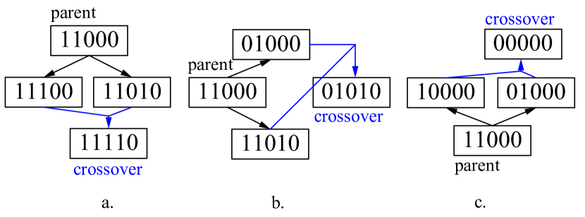
Figure 2: 3 types of cross over operations over the best and second best children of one parent. a. merge features from both children, equivalent to skip down; b. add one feature to one child, remove one feature from another child, equivalent to replace; c. remove one feature from each child, equivalent to skip up. All three operations can be represented by the simple arithmetic operation: $V_{crossover}$ = $V_{child1}$ + $V_{child2}$ - $V_{parent}$

After a node with the best score in the current queue is popped out, the BFS with crossover adds all its children to the priority queue. While this step is the same as Greedy BFS, a crossover operation is conducted between the best two children (“first” and “second” in Algorithm 2) of the node to identify a crossover node. This node is also added to the queue. There are three possible conditions depending on the relation of the two children with their parent (See Fig. 2).

Table II: Prediction performance using gradient boosting tree and different feature selection method. For the BFS method, the patience parameter is set to 25. For GBT, number of tree = 100, with depth searched from 2 to 5. Columns 2-6 are $r^{2}$ scores.

	Meta-heuristic	Greedy		Best First Search		BFS with Crossover Results
Test/Cohort	Genetic Algorithm	Forward	Backward	Greedy BFS	BFS with Crossover	Pearson Coefficient	p-value
DSF NC	0.4298	0.2074	-0.0649	0.4529	0.5055	0.75*	0.0109
DSB NC	0.4982	0.6200	0.2307	0.6408	0.6408	0.83*	0.0051
LNS NC	0.3599	0.4206	-0.1582	0.5182	0.5806	0.79*	0.0138
DSF mTBI	0.3510	0.3639	-0.3072	0.4396	0.5090	0.74**	0.0027
DSB mTBI	0.5186	0.5080	0.1321	0.5193	0.6005	0.80**	0.0005
LNS mTBI	0.5370	0.4749	-0.0763	0.5671	0.6036	0.82*	0.0013
DSF combine	0.2086	0.2895	-0.1444	0.3709	0.3848	0.64**	0.0019
DSB combine	0.2007	0.2089	-0.1592	0.4075	0.4491	0.69**	0.0018
LNS combine	0.2055	0.3931	0.1702	0.4813	0.4874	0.72***	0.0003

Compared to Greedy BFS, the crossover node, which is likely a good node with high score, will be evaluated with the same priority as all the children of the current node. With Greedy BFS, the crossover node will have to be evaluated along with all the children of the “first” node. With crossover, if the “cross” node is actually better than “first”, the evaluations of other children of “first” will be skipped. However, there is no guarantee that the “cross” node is better than the children node of “first”, so BFS with crossover may not always yield better results than Greedy BFS.

II-E Gradient Boosting Tree

Gradient boosting tree (GBT) is chosen as an estimator for its simplicity and robustness. The idea of boosting is to combine the output of many weak models to produce a powerful ensemble [24]. Gradient boosting adds the idea of steepest descent on top of boosting [25]. It iteratively adds new weak model to correct the largest previous error. In addition, decision tree is often chosen as a weak estimator. GBT has strong generalization ability and robustness to errors [24]. In our preliminary work, we have compared GBT with other regression methods including Support Vector Machine and Neural Network. For the $r^{2}$ result of Greedy DSB NC test, SVM and NN achieve $0.3455$ and $0.2501$ respectively, which is significantly lower than GBT ($0.6200$). Hence, we choose to present only the performance of GBT under different feature selection methods.

II-F Repeated Stratified K-fold Cross Validation

K-fold Cross-validation (CV) is widely applied method to estimate model performance [24]. Here, we use 5-fold cross validation with stratified CV split, which splits the entire dataset into 5 folds with the same distribution of labels [26][24]. In our case the labels are continuously distributed in $[-3,3]$. We quantize this range to 5 bins and each fold would have the same percentage of the samples in each bin, as the whole dataset.

III Results and Discussion

III-A Prediction results between BFS with Crossover and other heuristic algorithms

For each NP test, we develop three GBT models using control subjects, mTBI subjects, and all subjects, respectively. For each model, we perform feature selection using the proposed BFS with Crossover method as well as several other methods including greedy forward, greedy backward and genetic algorithm.

The average $r^{2}$ score among all validation samples is chosen to assess of model performance. $r^{2}$ is defined as the portion of variance explained:

$$r^{2}\leftarrow 1-\frac{MSE(y,\hat{y})}{Var(y)}$$ (6)

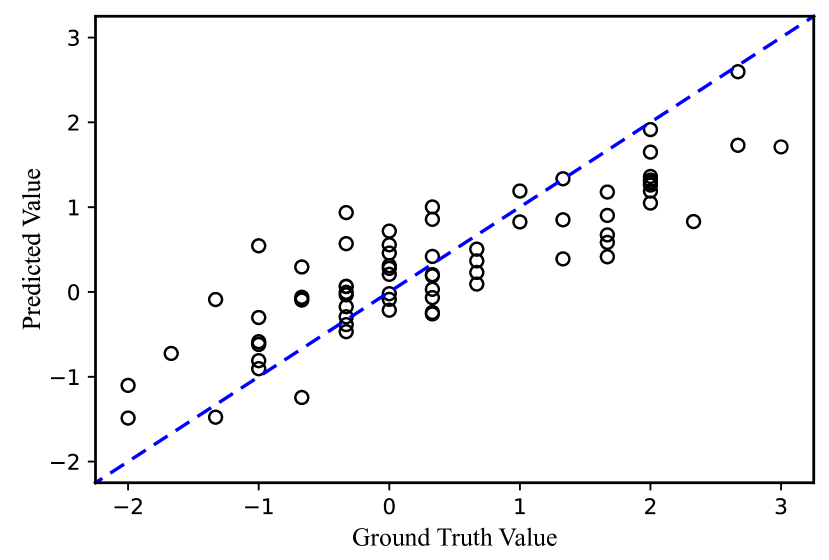
Figure 3: Comparison between ground truth label values and predicted label values for the DSB test, using the model developed for the mTBI population. Data shown here are from the validation samples in all five folds.

Table II summarizes the performance of different feature selection methods. Greedy backward search yields poor performance, suggesting that this is not a viable method when the feature space is very large. The greedy forward and genetic algorithm are substantially better than greedy backward, but the $r^{2}$ score is still mostly below 0.5 (See Tab. II). The Greedy BFS provides substantial improvement over these two methods in all the models. Finally, BFS with crossover achieves further improvement over greedy BFS in all cases, most of which yield $r^{2}$ scores above 0.5. Especially, the performance on DSB mTBI improves from 0.5193 by Greedy BFS to 0.6005 by BFS with crossover (See Tab. II). The relatively high $r^{2}$ scores and the scatter plot in Fig. 3 indicate a reasonably good fit.

Last two columns of Table II present the Pearson correlation between the ground truth and the predicted values by BFS with crossover and the corresponding p-value, which indicates the probability that an uncorrelated system produces such computed Pearson correlation. It could be observed that for most of the tests the Pearson correlation is larger than 0.7 with p value less than 0.05, which for biological systems indicates a strong and reliable relationship.

III-B Selected Features

Table III: Selected MRI Metrics by BFS with Crossover

Test/Cohort	Metrics Chosen Frequency
DSF NC	FA(5), De-perp(4), De-par(4), MK(2), AK(2), AWF(1), DA(1), MD(0)
DSB NC	De-par(3), De-perp(2), MK(2), FA(2), AK(2), MD(1), AWF(1), DA(0)
LNS NC	DA(4), AWF(3), De-perp(2), De-par(1), AK(1), MK(0), MD(0), FA(0)
NC SUM	De-perp(8), De-par(8), DA(5), AWF(5), AK(5), FA(5), MK(4), MD(1)
DSF mTBI	De-perp(5), De-par(4), AWF(3), MK(2), DA(2), AK(1), MD(0), FA(0)
DSB mTBI	AWF(10), AK(5), MK(3), FA(3), DA(2), MD(1), De-perp(1), De-par(0)
LNS mTBI	DA(6), AWF(3), De-par(3), AK(3), MK(2), MD(1), FA(1), De-perp(1)
mTBI SUM	AWF(16), DA(10), AK(9), De-perp(7), De-par(7), MK(7), FA(4), MD(2)
DSF combine	MD(5), DA(4), De-par(4), AWF(2), AK(2), FA(1), MK(0), De-perp(0)
DSB combine	AWF(4), DA(3), De-perp(3), MK(2), De-par(2), AK(2), MD(1), FA(1)
LNS combine	FA(5), AK(5), De-par(4), AWF(4), DA(2), De-perp(2), MK(1), MD(1)
combine SUM	AWF(16), DA(10), De-par(10), AK(9), De-perp(7), FA(7), MK(3), MD(2)

The features chosen by BFS with crossover are analyzed since they produce best accuracy. The number of times a diffusion MRI metric is chosen is accumulated and summarized in Table III.

For predicting the LNS test performance, it is interesting to observe that DA (Intra-axonal diffusivity, See Table I) metric is selected most often, for the modeled developed for the NC and mTBI cohorts, respectively. LNS is the most complex working memory task among these three tests and may have greater dependency on specific microstructural integrity more so than easy tasks. DA reflects axon injury or integrity and has been previously implicated in mTBI [5].

Additionally, it is noted that when counting the total number of times a metric is chosen over all three working memory tests, we see that for the models developed for the mTBI and control populations, respectively, the most frequently chosen features include De-par, De-perp, AWF, and DA. These compartment-specific metrics have been shown to be more sensitive to the underlying microstructure than others, such as DTI and DKI, which are known to be non-specific and empiric (See Table I).

Comparing the performances of separate models for the different cohorts (See Table II), we see that we are able to predict well with the models for the mTBI and NC cohorts, respectively. Furthermore, we see that the combined models (mTBI and NC together) are not as good with a weaker correlation coefficient for all three prediction tasks. The features chosen among these three populations for predicting the same NP score also differ (Table III). This suggests that mTBI and NP are two distinct populations in terms of white matter microstructure, in keeping with what we know about mTBI and white matter injury.

IV Conclusion

In this work, a new feature selection algorithm for predicting performance on working memory using diffusion MRI features is proposed. The algorithm is able to search over a large feature space effectively and achieved consistently better performance than other popular feature selection methods. This novel feature selection method is applicable to other classification and regression problems with large feature space and limited training data.

The prediction models using the selected features achieved quite high Pearson Correlation ($>0.7$ in all cases) with very low p-value ($<0.002$), demonstrating statistically significant agreement between the predicted scores and the measured working memory test scores. These results suggest that optimizing feature selection for predicting NP test performance has a great potential to reveal the most important imaging features that would be related to cognitive functions or cognitive impairments in mTBI patients.

References

- [1] M. Faul, M. M. Wald, L. Xu, and V. G. Coronado, “Traumatic brain injury in the united states; emergency department visits, hospitalizations, and deaths, 2002-2006,” 2010.
- [2] D. C. Voormolen, M. C. Cnossen, S. Polinder, N. Von Steinbuechel, P. E. Vos, and J. A. Haagsma, “Divergent classification methods of post-concussion syndrome after mild traumatic brain injury: prevalence rates, risk factors, and functional outcome,” Journal of neurotrauma, vol. 35, no. 11, pp. 1233–1241, 2018.
- [3] E. J. Grossman, M. Inglese, and R. Bammer, “Mild traumatic brain injury: is diffusion imaging ready for primetime in forensic medicine?” Topics in magnetic resonance imaging: TMRI, vol. 21, no. 6, p. 379, 2010.
- [4] M. E. Shenton, H. Hamoda, J. Schneiderman, S. Bouix, O. Pasternak, Y. Rathi, M.-A. Vu, M. P. Purohit, K. Helmer, I. Koerte et al., “A review of magnetic resonance imaging and diffusion tensor imaging findings in mild traumatic brain injury,” Brain imaging and behavior, vol. 6, no. 2, pp. 137–192, 2012.
- [5] S. Chung, E. Fieremans, X. Wang, N. E. Kucukboyaci, C. J. Morton, J. Babb, P. Amorapanth, F.-Y. A. Foo, D. S. Novikov, S. R. Flanagan et al., “White matter tract integrity: an indicator of axonal pathology after mild traumatic brain injury,” Journal of neurotrauma, vol. 35, no. 8, pp. 1015–1020, 2018.
- [6] S. Chung, X. Wang, E. Fieremans, R. Joseph, A. Prin, F. Farng-Yang A, C. Morton, N. Dmitry, F. Steven R, and Y. W. Lui, “Altered relationship between working memory and brain microstructure after mild traumatic brain injury,” American Journal of Neuroradiology, in press.
- [7] L. Miles, R. I. Grossman, G. Johnson, J. S. Babb, L. Diller, and M. Inglese, “Short-term dti predictors of cognitive dysfunction in mild traumatic brain injury,” Brain injury, vol. 22, no. 2, pp. 115–122, 2008.
- [8] Y. W. Lui, Y. Xue, D. Kenul, Y. Ge, R. I. Grossman, and Y. Wang, “Classification algorithms using multiple mri features in mild traumatic brain injury,” Neurology, vol. 83, no. 14, pp. 1235–1240, 2014.
- [9] S. Minaee, Y. Wang, and Y. W. Lui, “Prediction of longterm outcome of neuropsychological tests of mtbi patients using imaging features,” in 2013 IEEE Signal Processing in Medicine and Biology Symposium (SPMB). IEEE, Conference Proceedings, pp. 1–6.
- [10] S. Minaee, Y. Wang, A. Aygar, S. Chung, X. Wang, Y. W. Lui, E. Fieremans, S. Flanagan, and J. Rath, “Mtbi identification from diffusion mr images using bag of adversarial visual features,” IEEE transactions on medical imaging, 2019.
- [11] A. Makhzani, J. Shlens, N. Jaitly, I. Goodfellow, and B. Frey, “Adversarial autoencoders,” arXiv preprint arXiv:1511.05644, 2015.
- [12] P.-Y. Kao, E. Rojas, J. W. Chen, A. Zhang, and B. Manjunath, “Unsupervised 3-d feature learning for mild traumatic brain injury,” in International Workshop on Brainlesion: Glioma, Multiple Sclerosis, Stroke and Traumatic Brain Injuries. Springer, 2016, pp. 282–290.
- [13] J. Mitra, K.-k. Shen, S. Ghose, P. Bourgeat, J. Fripp, O. Salvado, K. Pannek, D. J. Taylor, J. L. Mathias, and S. Rose, “Statistical machine learning to identify traumatic brain injury (tbi) from structural disconnections of white matter networks,” NeuroImage, vol. 129, pp. 247–259, 2016.
- [14] R. Kohavi and G. H. John, “Wrappers for feature subset selection,” Artificial intelligence, vol. 97, no. 1-2, pp. 273–324, 1997.
- [15] J. M. Sattler and J. J. Ryan, Assessment with the WAIS-IV. Jerome M Sattler Publisher, 2009.
- [16] E. Fieremans, J. H. Jensen, and J. A. Helpern, “White matter characterization with diffusional kurtosis imaging,” Neuroimage, vol. 58, no. 1, pp. 177–188, 2011.
- [17] J. H. Jensen, E. T. McKinnon, G. R. Glenn, and J. A. Helpern, “Evaluating kurtosis-based diffusion mri tissue models for white matter with fiber ball imaging,” NMR in Biomedicine, vol. 30, no. 5, p. e3689, 2017.
- [18] G. Chandrashekar and F. Sahin, “A survey on feature selection methods,” Computers and Electrical Engineering, vol. 40, no. 1, pp. 16–28, 2014.
- [19] D. Rodrigues, L. A. Pereira, R. Y. Nakamura, K. A. Costa, X.-S. Yang, A. N. Souza, and J. P. Papa, “A wrapper approach for feature selection based on bat algorithm and optimum-path forest,” Expert Systems with Applications, vol. 41, no. 5, pp. 2250–2258, 2014.
- [20] J. E. Doran and D. Michie, “Experiments with the graph traverser program,” Proceedings of the Royal Society of London. Series A. Mathematical and Physical Sciences, vol. 294, no. 1437, pp. 235–259, 1966.
- [21] H. Arai, C. Maung, and H. Schweitzer, “Optimal column subset selection by a-star search,” in Twenty-ninth AAAI conference on artificial intelligence, 2015.
- [22] P. Pudil, J. Novovičová, and J. Kittler, “Floating search methods in feature selection,” Pattern recognition letters, vol. 15, no. 11, pp. 1119–1125, 1994.
- [23] J. Yang and V. Honavar, “Feature subset selection using a genetic algorithm,” in Feature extraction, construction and selection. Springer, 1998, pp. 117–136.
- [24] T. Hastie, R. Tibshirani, and J. Friedman, The Elements of Statistical Learning: Data Mining, Inference, and Prediction, ser. Springer Series in Statistics. Springer New York, 2013. [Online]. Available: https://books.google.com/books?id=yPfZBwAAQBAJ
- [25] J. H. Friedman, “Greedy function approximation: a gradient boosting machine,” Annals of statistics, pp. 1189–1232, 2001.
- [26] Y.-D. Zhang, Z.-J. Yang, H.-M. Lu, X.-X. Zhou, P. Phillips, Q.-M. Liu, and S.-H. Wang, “Facial emotion recognition based on biorthogonal wavelet entropy, fuzzy support vector machine, and stratified cross validation,” IEEE Access, vol. 4, pp. 8375–8385, 2016.