Constraining An Exact Brans-Dicke gravity theory with Recent Observations

Abstract

In this paper first we study Brans-Dicke equations with the cosmological constant to find an exact solution in the spatially flat Robertson-Walker metric. Then we use Observational Hubble data, the baryon acoustic oscillation distance ratio data as well as cosmic microwave background data from Planck to constrain parameters of the obtained Brans-Dicke model. To compare our results and find out the amount of deviation from general relativity, we also constrain concordance cosmological model using the same data. In our theoretical model the Brans-Dicke coupling constant is replaced by a , say new, parameter namely ‟scalar field density $\Omega_{\phi}$˝. Therefore, as $\Omega_{\phi}\to 0$ which is equivalent to $\omega\to\infty$ general relativity is recovered. In general, we found no significant deviation from general relativity. Our estimations show $\Omega_{\phi}=0.010^{+0.021}_{-0.012}$ which is equivalent to $\omega>1560$ at $95\%$ confidence level. We also obtained constraint the rate of change of gravitational constant, $\dot{G}/G$, at present time as $1.150\times 10^{-13}yr^{-1}<\dot{G}/G<1.198\times 10^{-13}yr^{-1}$ (at $1\sigma$ error). The total variation of gravitational constant, since the epoch of recombination, is also constrained as $-0.0084<\delta G/G<-0.0082$ at $68\%$ confidence level.

I Introduction

The concordance cosmological model ($\Lambda$CDM) of universe is credited today as the most simplest and successful cosmological model that describes the dynamics of present universe with acceleration but it suffers some fundamental problems on theoretical ground, which are reported by numerous cosmologists ref1 ; ref2 ; ref3 ; ref4 ; ref5 ; ref6 . The major cosmological constant problems are: fine tuning and cosmic coincidence which yet to be solve. Therefore, one may argue that the cosmological constant problem is the crisis of fundamental physics ref7 ; ref8 . It enforce cosmologist to think about the alternative of cosmological constant. This is why, in the literature various dark energy models with dynamical equation of state (EoS) parameter $\omega^{(eff)}$ have been studied (for example see ref9 ; ref10 ; ref11 ; ref12 ), where $\omega^{(eff)}=-1$ represents the $\Lambda$CDM universe ref13 ; ref14 . Some other proposals to avoid these conceptual problems associated with $\Lambda$ have been reported from time to time ref15 ; ref16 ; ref17 ; ref18 ; ref19 . However, to concur with high precision observational data, we have to have small deviation from $\Lambda$CDM model or modification to general theory of relativity but indeed, we still do not have a promising and concrete fundamental theory to handle this issue ref20 . In 1961, Brans-Dicke ref21 had proposed a scalar-tensor theory in which the average expansion rate is modified due to alignment of scalar field with geometry while the geometrization of tensor field remains alone ref22 . So, both the scalar and tensor field have more or less intrinsic geometrical consequences and finally executes a more general method of geometrizing gravitation. Other word, despite of Einstein’s general theory of relativity (GR), Brans-Dicke (BD) cosmology is not a fully geometrical theory of gravity. Brans-Dicke theory contains an additional parameter, the Brans-Dicke coupling $\omega$, as compared to GR. It should be noted that while large $\omega$ refers to as important contribution of the Ricci scalar, small $\omega$ indicates the main contribution of the scalar field. Since Einstein’s GR theory is recovered in the limit $\omega\to\infty$, BD theory could be considered as a good scale to quantify the accuracy of the predictions of GR against observational tests (reader is advised to see the textbooks, ref23 ; ref24 ). The value of $\omega$ could be estimated from the astronomical and astrophysical observational data. Using solar system data obtained from Cassini-Huygens mission, it is estimated $\omega>40000$ at $2\sigma$ confident level (CL) ref25 ; ref26 ; ref27 . Nevertheless, constraining $\omega$ using cosmological data obtained from WMAP and Planck missions gave lower values for this parameter. Wu and Chen combined cosmic microwave background (CMB) data from 5 years of WMAP, and LSS measurements from the Sloan Digital Sky Survey (SDSS) release 4 ref28 and obtained $\omega>97.8$ at $2\sigma$ CL. By using structure formation constraints, Acquaviva et al ref29 have obtained $\omega>120$ at $2\sigma$ CL. Li et al ref30 have used CMB temperature data from the Planck satellite, the 9 year polarization data from the WMAP and some others cosmological observations and found that $\omega$ varies in region $-407.0<\omega<175.87$ at $2\sigma$ CL. Hrycyna et al ref31 used supernovae type Ia and other cosmological data and found $\omega=\{-0.8606^{+0.8281}_{-0.1341},~{}-1.1103^{+0.1872}_{-0.1.729},~{}-2.3837^{+0.4588}_{-4.5459}\}$ for linear, oscillatory, and transient approaches to the de Sitter state respectively. Avilez and Skordis ref32 have reported strong cosmological constraints on coupling parameter of Brans-Dicke theory as $\omega>692$ by using CMB data. We recommend readers to see Refs ref33 ; ref34 ; ref35 for theoretical bounds on the Brans-Dicke coupling constant.

Generally, in the case of zero space curvature $(k=0)$ and zero pressure $(p=0)$ it is possible to find analytical solution for BD equations in the absence of the cosmological constant $\Lambda$ ref36 . However, since original BD model does not have accelerating expansion phase, it is convenient to extend this model by adding a $\Lambda$-term as an effective contribution rather than a potential (note that the precise shape of the scalar field potential is not known yet ref37 ). Some interesting BD solutions with a non-vanishing cosmological constant (henceforth $\Lambda$BD) could be found in Refs ref38 ; ref39 ; ref40 ; ref41 ; ref42 ; ref43 . In 1973 Gurevich et al ref44 obtained an exact analytical solution for pure BD with negative coupling constant, $\omega<0$, with no initial singularity. Since there is no cosmic acceleration in Gurevich et al solution, Tretyakova et al ref45 added a cosmological constant in order to extended Gurevich et al solution with negative $\omega$. They show that the scale factor may not vanish, unlike in the standard $\Lambda$CDM case. In 1984, Singh and Singh ref46 had investigated Brans-Dike cosmological model by choosing $\Lambda=\Lambda(\phi)$ and this idea was extended by Azad and Islam ref47 in an-isotropic and homogeneous Bianchi type I spacetime. A higher dimensional interacting scalar field and Higgs model is obtained by Qiang et al ref48 . Later on, using classical approach, Smolyakov ref49 has investigated Brans-Dike cosmological model with with effective value of $\Lambda$ in 5 D. Das and Banerjee ref50 have investigated model of accelerating universe with variable deceleration parameter in BD theory. In 2010, Setare and Jamil ref51 have constructed the chameleon model of holographic dark energy in BD theory and compared their results with those obtained via GR for large value of coupling constant $\omega$. In this connection, Yadav ref52 and Ali et al ref53 have investigated some non-isotropic, non-flat and in-homogeneous models of accelerating universe in BD scalar-tensor theory of gravitation. In this paper we obtain a new exact analytical solution for $\Lambda$BD model and use recent observational data namely CMB, BAO, and observational Hubble data (OHD) obtained from cosmic chronometric (CC) technique to constrain model parameters. It is worth mentioning that since in BD theory gravitational coupling $G$ is not a constant parameter, hence it’s variation means that supernovae can no longer be considered as standard candles (see Ref ref54 for more details). We use Metropolis-Hastings algorithm to generate Markov chain Monte Carlo (MCMC) chains and estimate model parameters. Although the main goal of this paper is to constrain $\omega$ (as we show in the next section, instead of BD coupling constant we introduce new density parameter i.e $\Omega_{\phi}$ and constrain this parameter) and $G$, but, we also discuses other important quantities such as deceleration and Hubble parameters. The plan of this paper is as follows: Section II deals with the model and basic equations. We summary the computational technique used to fit model parameters to data by a numerical MCMC analysis in SectionIII. Section  IV deals with the results of our fits to data. Finally, we summarize our findings in Section  V.

II Theoretical model and Basic equations

The Einstein’s field equations in Brans-Dicke theory with cosmological constant are given by

$$R_{ij}-\frac{1}{2}Rg_{ij}+\Lambda g_{ij}=\frac{8\pi}{\phi c^{2}}T_{ij}$$

$$-\frac{\omega}{\phi^{2}}\left(\phi_{i}\phi_{j}-\frac{1}{2}g_{ij}\phi_{k}\phi^{k}\right)-\frac{1}{\phi}(\phi_{ij}-g_{ij}\square\phi),$$ (1)

and

$$(2\omega+3)\square\phi=\frac{8\pi T}{c^{4}}+2\Lambda\phi,$$ (2)

where $\omega$ is the Brans-Dicke coupling constant; $\phi$ is Brans-Dicke scalar field and $\Lambda$ is the cosmological constant.
The FRW space-time is read as

$$ds^{2}=c^{2}dt^{2}-a^{2}(t)(dx^{2}+dy^{2}+dz^{2}),$$ (3)

where $a(t)$ is scale factor.
The energy momentum tensor of perfect fluid is given by

$$T_{ij}=(p+\rho)u_{i}u^{j}-pg_{ij}.$$ (4)

Here, $p$ and $\rho$ are the isotropic pressure and energy density of the matter respectively and $u^{i}u_{i}=1$; where $u^{i}$ is the four velocity vector.
The field equations (1) for space-time (3) are read as

$$2\frac{\ddot{a}}{a}+\frac{\dot{a}^{2}}{a^{2}}+\frac{\omega\dot{\phi}^{2}}{2\phi^{2}}+2\frac{\dot{\phi}\dot{a}}{\phi a}+\frac{\ddot{\phi}}{\phi}=-\frac{8\pi}{\phi c^{2}}p+\Lambda c^{2},$$ (5)

$$\frac{\dot{a}^{2}}{a^{2}}+\frac{\phi\dot{a}}{\phi a}-\frac{\omega\dot{\phi}^{2}}{6\phi^{2}}=\frac{8\pi}{3\phi c^{2}}\rho+\frac{\Lambda c^{2}}{3},$$ (6)

$$\frac{\ddot{\phi}}{\phi}+3\frac{\dot{\phi}\dot{a}}{\phi a}=\frac{8\pi(\rho-3p)}{(2\omega+3)c^{2}\phi}+\frac{2\Lambda c^{2}}{2\omega+3}.$$ (7)

In this paper we use over dot to show derivatives with respect to time $t$.

Equations (5), (6) and (7) lead the following equation

$$\Lambda c^{2}=3\frac{\ddot{a}}{a}+3\frac{\dot{a}^{2}}{a^{2}}-\omega\frac{\ddot{\phi}}{\phi}-3\omega\frac{\dot{\phi\dot{a}}}{\phi a}+\frac{\omega\dot{\phi}^{2}}{\phi^{2}}.$$ (8)

Before solving above questions we define the matter and cosmological constant density parameters as

$$\Omega_{m}=\frac{8\pi\rho_{m}}{3c^{2}H^{2}\phi},~{}~{}\Omega_{\Lambda}=\frac{\Lambda c^{2}}{3H^{2}},$$ (9)

where $\rho_{m}=\left(\rho_{m}\right)_{0}a^{-3}$ and $\{\Omega_{m},\Omega_{\Lambda}\}$ stand for matter and $\Lambda$-term density parameters respectively. We also define the deceleration parameter (DP) $q$ and the scalar field deceleration parameter $q_{\phi}$ as bellow

$$q=-\frac{\ddot{a}}{aH^{2}}~{}~{}~{}q_{\phi}=-\frac{\ddot{\phi}}{\phi H^{2}}.$$ (10)

Now, dividing equations (6) by $H^{2}$ and then using equation (9), we obtain

$$\Omega_{m}+\Omega_{\Lambda}=1+\psi-\frac{\omega}{6}\psi^{2},$$ (11)

where $\psi=\frac{\dot{\phi}}{\phi H}$. It should be noted that in BD gravity theory one can not use the usual relation between Hubble parameter and density in order to define density parameters, meaning that for a spatially-flat model the sum of density parameters don’t quite sum to one.

We assume that the present universe is filled with pressure-less matter i. e. $p=0$. So, putting $p=0$ in equations (5), (7) and (8) then dividing by $3H^{2}$ and using equations (9) and (10), we obtain the following relations

$$\Omega_{\Lambda}=\frac{\omega+3}{2\omega}\Omega_{m}-\frac{2\omega+3}{2\omega}q+\frac{2\omega+3}{6}\psi^{2}-\frac{2\omega+3}{2\omega}\psi,$$ (12)

$$1-\frac{3(\omega+1)}{2\omega}\Omega_{m}+\frac{2\omega+3}{2\omega}q+\frac{4\omega+3}{2\omega}\psi-\frac{\omega+1}{2}\psi^{2}=0,$$ (13)

$$\Omega_{m}=q-\frac{\omega}{3}q_{\phi}+(\omega+1)\psi-\frac{\omega}{3}\psi^{2}.$$ (14)

Equations (13) and (14) lead to

$$q-(\omega+1)q_{\phi}+(3\omega+2)\psi=2.$$ (15)

The first integral of equation (15) is read as

$$(\omega+1)\frac{\dot{\phi}}{\phi}-\frac{\dot{a}}{a}=\frac{\kappa}{\phi a^{3}},$$ (16)

where $\kappa$ is the constant of integration.

The solution of equation (16) has singularity at $a=0$ and $\phi=0$ which in turn gives $\kappa=0$. Thus equation (16) could be written as

$$(\omega+1)\frac{\dot{\phi}}{\phi}-\frac{\dot{a}}{a}=0.$$ (17)

Integrating equation (17), finally we obtain

$$\phi=\left(\frac{a}{a_{0}}\right)^{\frac{1}{\omega+1}}.$$ (18)

Dividing equation (17) by $H$ and then integrating, we obtain

$\psi=\frac{1}{\omega+1}$.

Thus, equation (11) leads to

$$\Omega_{m}+\Omega_{\Lambda}=1+\frac{5\omega+6}{6(\omega+1)^{2}}.$$ (19)

If we define the density of scalar field $\phi$ as

$$\Omega_{\phi}=-\frac{5\omega+6}{6(\omega+1)^{2}},$$ (20)

then eq (19) is written as

$$\Omega_{m}+\Omega_{\Lambda}+\Omega_{\phi}=1.$$ (21)

The scale factor $a$ and $\phi$ in connection with redshift $z$ are read as

$$a=\frac{a_{0}}{1+z},~{}~{}\phi=\frac{1}{(1+z)^{\frac{1}{1+\omega}}}=\frac{1}{(1+z)^{2.5(\sqrt{1+0.96\Omega_{\phi}}-1)}},$$ (22)

where $a_{0}$ is the present value of scale factor.

Equations (9), (21) and (22) leads to

$$H_{BD}=\frac{H_{0}}{(1-\Omega_{\phi})^{\frac{1}{2}}}\left[\Omega_{m}(1+z)^{3+2.5(\sqrt{1+0.96\Omega_{\phi}}-1)}+\Omega_{\Lambda}\right]^{\frac{1}{2}},$$ (23)

where $H_{0}$ is the present value of Hubble’s parameter. Above equation clearly imposes a lower bound on the scalar field density as $\Omega_{\phi}\geq-1.04$. It is also interesting to note that, now, $\Omega_{\phi}\to 0$ is equivalent to $\omega\to\infty$ for which GR recovers from BD gravity theory. Obviously, as $\Omega_{\phi}\to 0$, $\Lambda$CDM model recovers from eq (23)

$$H_{\Lambda CDM}=H_{0}[\Omega_{m}(1+z)^{3}+\Omega_{\Lambda}]^{\frac{1}{2}}.$$ (24)

We also note that a de-Sitter solution arises whenever

$$q=-1\Rightarrow\dot{H}=0\Rightarrow H=H_{0}\Rightarrow a(t)\propto e^{H_{0}t}.$$ (25)

Since for our $\Lambda$BD model we have

$$q_{z=0}=\frac{\Omega_{m}\left(\sqrt{24\Omega_{\phi}+25}-3\right)-4\Omega_{\Lambda}}{4\left(\Omega_{\Lambda}+\Omega_{m}\right)},$$ (26)

it is clear to conclude that this condition can not be achieved in our $\Lambda$BD model (see APPENDIX A for derivation of DP an transition redshift).
In the next section we use joint combination of three independent observational data including OHD, BAO, CMB to constrain both $\Lambda$CDM and $\Lambda$BD models with following parameters space

$${\bf\Theta_{\Lambda CDM}}=\{H_{0},\Omega_{m},\Omega_{\Lambda},\Omega_{b}h^{2},t(Gyr),q_{0}\},$$ (27)

and

$${\bf\Theta_{\Lambda BD}}=\{H_{0},\Omega_{m},\Omega_{\Lambda},\Omega_{b}h^{2},t(Gyr),q_{0},\Omega_{\phi},\dot{G}/G\}.$$ (28)

Note that $\Lambda$CDM model has only two free parameters i.e $\{H_{0},\Omega_{m}\}$ while $\Lambda$BD model has three free parameters namely $\{H_{0},\Omega_{m},\Omega_{\phi}\}$, hence, all other parameters are derived parameters.

III Data and Method

We use Metropolis-Hasting algorithm from the Pymc3 python package to generate MCMC chains for parameter spaces (27) and (28). For each parameter we run 4 parallel chains with 100000 iterations to stabilize the estimations. In order to confirm the convergence of the MCMC chains we perform well known Gelman-Rubin and Geweke tests. Moreover, we monitor the trace plots for good mixing and stationarity of the posterior distributions to confirm the convergence of all chains. In our Bayesian analysis, we assume the following uniform priors for free parameters:

$$H_{0}\sim U(60-800)~{}~{}~{}\Omega_{m}\sim U(0-0.5)~{}~{}~{}\Omega_{\phi}\sim U(-0.5-0.5).$$ (29)

In bellow we briefly describe the cosmological data we have been used to constrain parameter spaces (27) and (28).
Observational Hubble Data: we use $31H(z)$ datapoints (Table. 1) in the redshift range $.07\leq z\leq 1.965$ taken from Table 2 of Ref ref55 . The cosmic chronometric (CC) technique is used to determined these uncorrelated data. There reason why we use this data is behind the fact that OHD data obtained from CC technique is model-independent. In fact, the most massive and passively evolving galaxies based on the “galaxy differential age”method is used to determine the CC data (see refref56 for more details). Since in this compilation all data are uncorrelated, we consider ${\bf C_{ij}}=\mbox{diag}(\sigma_{i}^{2})$ as covariance matrix of this class of data. The chisqure for this data is given by

$$\chi^{2}_{HOD}=(H(z)-H_{0})^{T}{\bf C}^{-1}(H(z)-H_{0}),$$ (30)

Table 1: Hubble parameter versus redshift data.

$H(z)$	$\sigma_{H}$	$z$	Reference
69	19.6	0.070	ref57
69	12	0.090	ref58
68.6	26.2	0.120	ref57
83	8	0.170	ref58
75	4	0.179	ref59
75	5	0.199	ref59
72.9	29.6	0.200	ref57
77	14	0.270	ref58
88.8	36.6	0.280	ref57
83	14	0.352	ref59
83	13.5	0.3802	ref60
95	17	0.400	ref58
77	10.2	0.4004	ref60
87.1	11.2	0.4247	ref60
92.8	12.9	0.4497	ref60
89	50	0.47	ref61
80.9	9	0.4783	ref60
97	62	0.480	ref62
104	13	0.593	ref59
92	8	0.680	ref59
105	12	0.781	ref59
125	17	0.875	ref59
90	40	0.880	ref62
117	23	0.900	ref58
154	20	1.037	ref59
168	17	1.300	ref58
160	33.6	1.363	ref63
177	18	1.430	ref58
140	14	1.530	ref58
202	40	1.750	ref58
186.5	50.4	1.965	ref63

CMB: It is shown ref64 that the existence of dark energy could affect CMB power spectrum in at least two ways. First, the change of the angular diameter distance causes a shift in positions of CMB acoustic peaks from the last scattering surface to today. Second, the presence of dark energy results in fluctuation of gravitational potentials which in turn leads to the late-time integrated Sachs-Wolfe effect. As the first effect is more important to constrain dark energy models, we only use CMB distance measurements in our statistical analysis. In this regard, we consider following two CMB shift parameters (for flat space-time).

$$R=\sqrt{\Omega_{m}}\int_{0}^{z_{\ast}}\frac{dz}{E(z)},$$ (31)

and

$$l_{a}=\frac{\pi r(z_{\ast})}{r_{s}(z_{\ast})},$$ (32)

while the average acoustic structure is determined by the acoustic scale $l_{a}$, the shift parameter $R$ is associated with the overall amplitude of CMB acoustic peak. In eq (32) the comoving distance to the CMB decoupling surface $r(z_{\ast})$ and the comoving sound horizon at the CMB decoupling $r_{s}(z_{\ast})$ are given by

$$r(z_{\ast})=\int_{0}^{z_{\ast}}\frac{dz}{H(z)},~{}~{}r_{s}(z_{\ast})=\frac{1}{H_{0}}\int_{z}^{\infty}\frac{dz^{\prime}c_{s}(z^{\prime})}{E(z^{\prime})},$$ (33)

where $E(z)^{2}=H(z)/H_{0}$, and the sound speed squared $c_{s}$ of baryon fluid coupled with photons ($\gamma$) is given by ref65

$$c_{s}=\frac{1}{\sqrt{3[1+R_{b}/(1+z)]}},~{}~{}R_{b}=31500\Omega_{b}h^{2}\left(\frac{2.7255}{2.7}\right)^{-4},$$ (34)

where $h$ is the normalized Hubble constant and $z_{\ast}=1090$ is decoupling redshift. We use the CMB distance priors based and Planck 2015 collaboration ref3 to constrain our models. According to Planck 2015 data, the mean values of shift and acoustic scale parameters are $\langle R\rangle=1.7488$ and $\langle l_{a}\rangle=301.76$ with the deviations $\sigma(R)=0.0074$ and $\sigma(l_{a})=0.14$ respectively. For this data, the inverse of the covariance matrix is given by

$$\mathbf{C}^{-1}=\begin{pmatrix}1.412&-0.762\\[0.86108pt] -0.762&1.412\end{pmatrix}.$$ (35)

Finally, The chisquare associated with the CMB data could be obtained as

$$\chi_{CMB}^{2}=(l_{a}-301.76)^{2}\times 1.412+(R-1.7488)^{2}\times 1.412$$

$$+2(l_{a}-301.76)(R-1.7488)\times(-0.762).$$ (36)

BAO: The counteracting forces of pressure and gravity result in periodic fluctuations of the density of baryonic matter which represent by BAO. We use almost the same BAO data points were used in the WMAP 9-year analysis ref66 . This includes ten numbers of $r_{s}(z_{d})/D_{V}(z)$ extracted from the 6dFGS ref67 , SDSS-MGS ref68 , BOSS ref69 , BOSS CMASS ref70 , and WiggleZ ref71 surveys. Here $D_{V}(z)$ which is given by

$$D_{V}(z)=\left[r^{2}(z)\frac{cz}{H(z)}\right]^{\frac{1}{3}},$$ (37)

is the effective distance measure related to the BAO scale ref72 , $c$ is the speed of light, and $r_{s}(z_{d})$ is the comoving sound horizon size at the drag epoch. The drag redshift $z_{d}$, which is the redshift at which baryons are released from photons has the following fitting formula ref73

$$z_{d}=\frac{1291(\Omega_{m}h^{2})^{0.251}}{1+0.659(\Omega_{m}h^{2})^{0.828}}[1+b_{1}(\Omega_{b}h^{2})^{b_{2}}],$$ (38)

where

$$b_{1}=0.313(\Omega_{m}h^{2})^{-0.419}[1+0.607(\Omega_{m}h^{2})^{0.674}],$$ (39)

and

$$b_{2}=0.238(\Omega_{m}h^{2})^{0.223}.$$ (40)

The chisquare statistics for BAO could be written as

$$\chi^{2}_{BAO}=\\ \frac{1}{0.015^{2}}\left[\frac{r_{s}(z_{d})}{D_{V}(z=0.106)}-0.336\right]^{2}+\frac{1}{(\frac{25}{149.69})^{2}}\left[\frac{D_{V}(z=0.15)}{r_{s}(z_{d})}-\frac{664}{148.69}\right]^{2}+\frac{1}{(\frac{25}{149.28})^{2}}\left[\frac{D_{V}(z=0.32)}{r_{s}(z_{d})}-\frac{1264}{149.28}\right]^{2}\\ +\frac{1}{(\frac{16}{147.78})^{2}}\left[\frac{D_{V}(z=0.38)}{r_{s}(z_{d})}-\frac{1477}{147.78}\right]^{2}+\frac{1}{0.0071^{2}}\left[\frac{r_{s}(z_{d})}{D_{V}(z=0.44)}-0.0916\right]^{2}+\frac{1}{(\frac{19}{147.78})^{2}}\left[\frac{D_{V}(z=0.51)}{r_{s}(z_{d})}-\frac{1877}{147.78}\right]^{2}\\ +\frac{1}{(\frac{20}{149.28})^{2}}\left[\frac{D_{V}(z=0.57)}{r_{s}(z_{d})}-\frac{2056}{149.28}\right]^{2}+\frac{1}{0.0034^{2}}\left[\frac{r_{s}(z_{d})}{D_{V}(z=0.6)}-0.0726\right]^{2}+\frac{1}{(\frac{22}{147.78})^{2}}\left[\frac{D_{V}(z=0.61)}{r_{s}(z_{d})}-\frac{2140}{147.78}\right]^{2}\\ +\frac{1}{0.0032^{2}}\left[\frac{r_{s}(z_{d})}{D_{V}(z=0.73)}-0.0592\right]^{2}$$ (41)

Finally, since these three datasets are independent, the total chisqure could be given by $\chi^{2}_{tot}=\chi^{2}_{OHD}+\chi^{2}_{CMB}+\chi^{2}_{BAO}$. Therefore, we evaluated the following total likelihood for statistical analysis.

$$\mathcal{L}_{tot}\propto\exp\left(-\frac{1}{2}\chi^{2}_{tot}\right).$$ (42)

IV Results

We have listed our statistical analysis on parameter spaces (27) & (28) using the joint combination of OHD+CMB+BAO at 1$\sigma$ and $2\sigma$ error in Table. 2. Also, Figures. 1 & 2 show the contour plots, at $1\sigma$, $2\sigma$, and $3\sigma$ confidence levels, for both $\Lambda$BD and $\Lambda$CDM models using joint combination of three datasests respectively. First we discuss the $\Lambda$BD model, which contain $\omega$ as an additional parameter to $\Lambda$CDM model. From Table. 2 we observe that $\Omega_{\phi}$ is restricted in the interval $0.0001<\Omega_{\phi}<0.0127$ at $1\sigma$ CL with the best fit $\Omega_{\phi}=0.0027$, which in turn gives the best fit for BD constant parameter as $\omega=308.452$. Our analysis show that the BD parameter is constrained to $\omega>\{211,1560,8460\}$ at $68\%,~{}95\%$, and $~{}99\%$ confidence level respectively. We have compared our result of $\omega$ to those obtained from other researches in Table. 3. From this table we observe that our estimated bound on $\omega$ is much stronger than those reported by previous works. While our computed $\omega$ is comparable with that obtained by Avilez and Skordis ref32 at $95\%$ CL, but our analysis put much stronger bound on this parameter at $99$ CL. Also at $68\%$ CL our obtained bound is comparable with what computed by Li et alref30 . Figures. 3 shows the $1\sigma$-$3\sigma$ contour plot of $(\omega,H_{0})$ pair.

Table 2: Results from the fits of the flat $\Lambda$CDM and $\Lambda$BD models to the data at $2\sigma$ & $2\sigma$ confidence levels.

		Parameter	$\%68$	$\%95$	Best Fit
$\Lambda$CDM	Fit	$H_{0}$	$68.68\pm 0.62$	$68.7^{+1.2}_{-1.2}$	$67.90$
		$\Omega_{m}$	$0.3290\pm 0.0089$	$0.329^{+0.018}_{-0.017}$	$0.344$
	Derived	$\Omega_{\Lambda}$	$0.6710\pm 0.0089$	$0.671^{+0.017}_{-0.018}$	$0.655$
		$\Omega_{b}h^{2}$	$0.02322\pm 0.00042$	$0.02322^{+0.00086}_{-0.00079}$	$0.023$
		$Age(Gyr)$	$13.56\pm 0.13$	$13.56^{+0.27}_{-0.25}$	$13.73$
		$q$	$-0.507\pm 0.013$	$-0.507^{+0.027}_{-0.025}$	$-0.482$
$\Lambda$BD	Fit	$H_{0}$	$68.78\pm 0.62$	$68.8^{+1.2}_{-1.2}$	$69.334$
		$\Omega_{\phi}$	$0.0101^{+0.0026}_{-0.010}$	$0.010^{+0.021}_{-0.012}$	$0.0027$
		$\Omega_{m}$	$0.321^{+0.012}_{-0.0096}$	$0.321^{+0.023}_{-0.024}$	$0.318$
	Derived	$\Omega_{\Lambda}$	$0.6692\pm 0.0089$	$0.669^{+0.017}_{-0.018}$	$0.678$
		$\omega$	$>211$	$>1560$	$308.452$
		$\Omega_{b}h^{2}$	$0.02315\pm 0.00042$	$0.02315^{+0.00084}_{-0.00081}$	$0.0227$
		$Age(Gyr)$	$13.38\pm 0.12$	$13.38^{+0.24}_{-0.23}$	$13.246$
		$\frac{\dot{G}}{G}(10^{-12}yr^{-1})$	$0.1147\pm 0.0024$	$0.1147^{+0.0046}_{-0.0046}$	$0.117$
		$q$	$-0.585\pm 0.016$	$-0.585^{+0.032}_{-0.032}$	$-0.595$

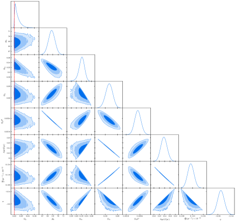
Figure 1: One-dimensional marginalized distribution, and three-dimensional contours with $68\%$ CL, $95\%$ CL, and $99\%$ CL for parameter space $\Theta_{\Lambda DB}$ using CC+ABO+CMB data. The vertical dashed red line stands for $\Omega_{\phi}=0$.

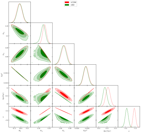
Figure 2: One-dimensional marginalized distribution, and two-dimensional contours with $68\%$ CL, $95\%$, and $99\%$ CL for flat $\Lambda$CDM and $\Lambda$BD models fitted over CC+ABO+CMB data.

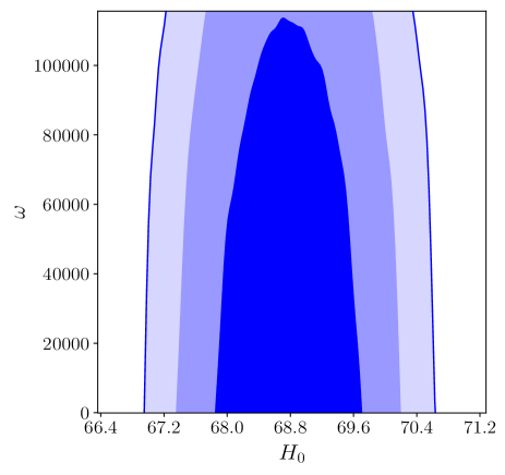
Figure 3: Constraints in the $(\omega,H_{0})$ plane with $1\sigma$-$3\sigma$ confident level in the flat $\Lambda$BD model fitted over CC+ABO+CMB data.

Table 3: Constraints on the BD coupling constant from different researches.

BD parameter	Method
$\omega>\{80(3\sigma),120(2\sigma)\}$	CMB+WMAP+LSS	ref29
$\omega>97.8(2\sigma)$	WMAP5+SDSSLRG	ref74
$\omega>\{337.34(1\sigma),181.65(2\sigma)\}$	WMAP9pol+BAO	ref30
$\omega>\{1834(2\sigma),890(3\sigma)\}$	PLANCKTEMP+WMAP9pol	ref32
$\omega>\{211(1\sigma),1560(2\sigma),8460(3\sigma)\}$	CC+CMB+BAO	This paper

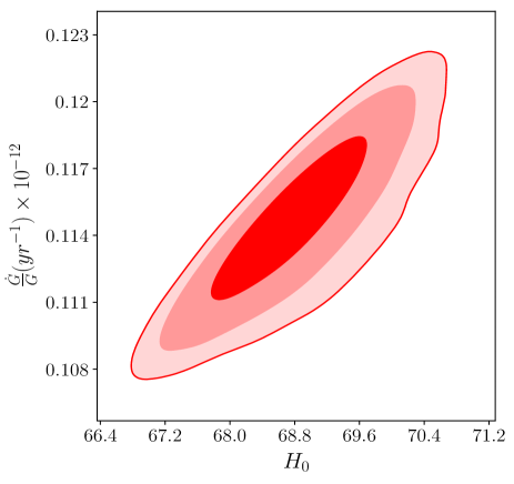
Figure 4: Constraints in the $(\dot{G}/G,H_{0})$ plane with $1\sigma$-$3\sigma$ confident level.

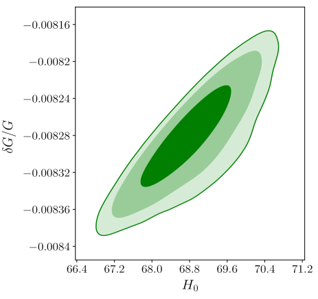
Figure 5: Constraints in the $(\delta G/G,H_{0})$ plane with $1\sigma$-$3\sigma$ confident level.

We know that in the context of BD theory, the gravitational constant $G$ is also underwent evolution from recombination era to the current time ref73 . Therefor, one can estimate the variation in $G$ throughout variations of $\Omega_{\phi}~{}\mbox{or}~{}\omega$ as these two parameters are correlated. For this purpose, we inter two new derived parameters namely $\dot{G}/G\equiv-\dot{\phi}/\phi$ and $\delta G/G\equiv(G_{rec}-G_{0})/G_{0}$ which is the integrated change of gravitational constant since the epoch of recombination in our MCMC code. Figures. 4 & 5 depict 2-dimensional contours of marginalized likelihood distributions of $H_{0}$ versus $\dot{G}/G$ and $\delta G/G$ respectively. The $68$% marginalized limits on these two parameters are as bellow.

$$1.150\times 10^{-13}<\dot{G}/G<1.198\times 10^{-13},$$

$$-0.0084<\delta G/G<-0.0082,$$ (43)

with the best-fit values

$$\dot{G}/G=1.17\times 10^{-13},~{}~{}\delta G/G=-0.00825.$$ (44)

We have summarized constraints on $\dot{G}/G$ obtained from different methods in Table. 4 which is an update of Table I of Ref ref30 . From this table we observe that our constrain is much tighter with respect to other listed previous constraints.

Table 4: Constraints on the BD coupling constant from different researches.

$\dot{G}/G(10^{-13}yr^{-1})$	Method
$2\pm 7$	Lunar laser ranging	ref75
$0\pm 4$	Big bang nucleosynthesis	ref76 ; ref77
$0\pm 16$	Helioseismology	ref78
$-6\pm 20$	Neutron star mass	ref79
$20\pm 40$	Viking lander ranging	ref80
$40\pm 50$	Binary pulsar	ref81
$-96\sim 81(2\sigma)$	CMB(WMAP3)	ref82
$-17.5\sim 10.5(2\sigma)$	WMAP5+SDSSLRG	ref74
$-1.42^{+2.48+4.38}_{-2.27-4.74}(1\sigma 2\sigma)$	Planck+WP+BAO	ref30
$1.174^{+0.0024+0.0046}_{-0.0024-0.0046}(1\sigma 2\sigma)$	CC+CMB+BAO	This paper

From Table. 2 we see that the estimated Hubble constant $H_{0}$ for both $\Lambda$CDM and $\Lambda$BD models are in excellent agreement with those of Chen & Ratra ($68\pm 2.8$) ref83 , Aubourg et al (BAO: $67.3\pm 1.1$) ref84 , Chen et al ($68.4^{+2.9}_{-3.3}$) ref85 , Aghanim et al (Planck 2018: $67.66\pm 0.42$) ref4 , and 9-years WMAP mission ($68.92^{+0.94}_{-0.95}$) ref86 . Figure. 6 depicts the robustness of our fits for $H(z)$. When we fit both $(\Theta_{\Lambda CDM},\Theta_{\Lambda BD})$ to CC+CMB+BAO data we obtain $(\Omega_{m}=0.329\pm 0.0089,\Omega_{\Lambda}=0.671\pm 0.0089)$ and $(\Omega_{m}=0.321^{+0.012}_{-0.0096},\Omega_{\Lambda}=0.669\pm 0.0089)$ for these models respectively. Obviously, these results are in excellent agreement with those obtained by Planck 2018 collaborationref4 ($\Omega_{m}=0.3103\pm 0.0057,\Omega_{\Lambda}=0.6897\pm 0.0057$).

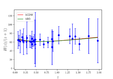
Figure 6: The plot of Hubble rate versus the redshift $z$. The points with bars indicate the experimental data summarized in Table. 1

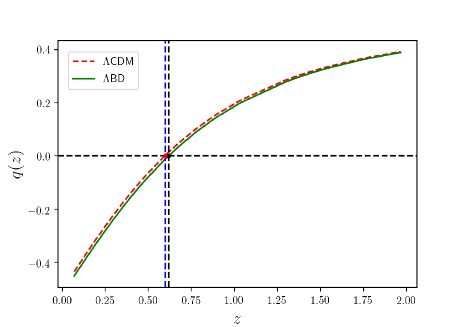
Figure 7: The plot of deceleration parameter versus the redshift $z$ for Both $\Lambda$CDM & $\Lambda$BD models. Filled circles show the best fit values of DP at transition red-shift $z_{t}$.

The computed values of deceleration parameter for $\Lambda$CDM & $\Lambda$BD models are $q_{\Lambda CDM}=-0.507^{+0.013+0.027+0.07}_{-0.013-0.025-0.032}$ and $q_{\Lambda BD}=-0.585^{+0.016+0.032+0.042}_{-0.016-0.032-0.044}$ at $1\sigma-2\sigma$ respectively. Our estimated values of DP for both models are in good agreement with those reported in Refs ref87 , ref88 , ref89 , and ref90 . The dependence of deceleration parameter $q(z)$ has been plotted in Figures. 7 as a function of redshift $z$. Our computations show that both $\Lambda$BD & $\Lambda$CDM models inters the accelerating expansion phase almost at the same time (also see fig. 7). We also estimated transition redshift $z_{t}$ for both models as a derived parameter in our MCMC code. We found $z_{t}=0.602^{+0.021+0.041+0.054}_{-0.021-0.041-0.055}$ for $\Lambda$BD and $z_{t}=0.599^{+0.021+0.041+0.055}_{-0.021-0.041-0.054}$ for $\Lambda$CDM models at $1\sigma-3\sigma$ CL. Figure. 8 shows the $1\sigma-3\sigma$ contour plot of ($H_{0}-z_{t}$) pair. It has recently been shown ref91 that the transition redshift should be restricted in a specific interval as $0.33<z_{t}<1$. For Both models, the computed $z_{t}$ is in good agreement with those obtained in Refsref92 ; ref93 ; ref94

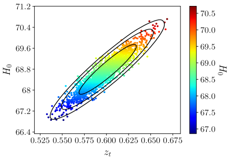
Figure 8: $H_{0}-z_{t}$ plane with $1\sigma-3\sigma$ confident level. Solid contours stand for $\Lambda$BD model

V Concluding Remarks

In this paper first we tried to obtain a new exact solution for Brans-Dicke equations with the cosmological constant in the spatially flat Robertson-Walker metric. We defined new density parameter for scalar field i.e $\Omega_{\phi}$ which recovers GR theory when tends to zero (this is ,of course, equivalent to the case when $\omega\to\infty$). The latest observational data namely OHD (CC data), CMB, and BAO have been used to constrain parameter spaces 28 (Brans-Dicke theory) & 27 (General relativity theory). To this aim, We have used Metropolis-Hasting algorithm to perform MCMC analysis. The marginalized bounds on BD coupling constant are obtained as $\omega>(211,1560)$ at $68\%$ and $95\%$ confident levels respectively. Our estimations put tighten constrain on the Brans-Dicke model compared with previous works. Moreover, we defined two additional derived parameters in MCMC code namely the rate of change of the gravitational constant $\dot{G}/G$ and the integrated change of this parameter $\delta G/G$ since the epoch of recombination to explore whether $G$ is a ‟constant˝or not. The marginalized $1\sigma$ limits are given by equation 43. These bounds are in excellent agreement with the precision of Solar System experiments. Generally, our computations do not show any significant deviation from general theory of relativity. When we compare the distribution of other cosmological parameters of 28 & 27 spaces, we find out that the introduction of Brans-Dicke gravity does not affect the best-fit values and estimated errors.

APPENDIX A

It is well known that at a specific redshift called transition, $z_{t}$ the expansion phase of universe changes from decelerating to accelerating. To obtain this special redshift, first we derive deceleration parameter which is defined as

$$q(z)=-\frac{1}{H^{2}}\left(\frac{\ddot{a}}{a}\right)=\frac{(1+z)}{H(z)}\frac{dH(z)}{dz}-1.$$ (A1)

Using 23 in above equation, and after some algebra we obtain

$$q(z)=\frac{\Omega_{m}(\sqrt{24\Omega_{\phi}+25}-3)(1+z)^{\frac{1}{2}(\sqrt{24\Omega_{\phi}+25}+1)}}{4\left[\Omega_{\Lambda}+\Omega_{m}(1+z)^{\frac{1}{2}(\sqrt{24\Omega_{\phi}+25}+1)}\right]}.$$ (A2)

In the other hand, transition redshift could be defined by the condition $q(z_{t})=\ddot{a}(z_{t})=0$. Applying this condition in above equation and after some algebra finally we get transition redshift as follows.

$$z_{t}=\left[\frac{4\Omega_{\Lambda}}{\Omega_{m}(\sqrt{24\Omega_{\phi}+25}-3)}\right]^{\frac{2}{\sqrt{24\Omega_{\phi}+25}+1}}-1.$$ (A3)

It is straightforward to show that in flat-$\Lambda$CDM model the transition redshif is given by

$$z_{t}=\left(\frac{2\Omega_{\Lambda}}{\Omega_{m}}\right)^{\frac{1}{3}}-1.$$ (A4)

References

- (1) O. Akarsu et al. arXiv: 1903.06679v1 [gr-qc] (2019).
- (2) E. Komastu et al. Astrophys. J. Suppl. Ser. 192, 18 (2011).
- (3) P. A. R. Ade et al. Astron. Astrophys. 594, A13 (2016).
- (4) N. Aghamin et al. [Plank Collaboration], arXiv: 1807.06209 [astro-ph.CO] (2018).
- (5) P. J. E. Peebles and B. Ratra, Rev. Mod. Phys. 75, 559 (2003)
- (6) T. Padmanabhan, Phys. Rept. 380, 234 (2003)
- (7) S. Weinberg, Rev. Mod. Phys. 61, 1 (1989)
- (8) P.J.E. Peebles, B. Ratra, Rev. Mod. Phys. 75, 559 (2003)
- (9) V. Sahni, A. Shafieloo and A. A. Starobinsky, Astrophys. J. 793, 2 (2014)
- (10) A. Shafieloo, B. L. Huillier and A. A. Starobinsky, Phys. Rev. D 98, 083526 (2018)
- (11) A. K. Yadav, Astrophys. Space Sc. 335,565 (2011)
- (12) A. K. Yadav, Astrophys. Space Sc. 361,276 (2016)
- (13) G. K. Goswami, Research in Astron. Astrophys. 17, 27 (2017); arXiv: 1710.0728 [gr-qc] (2017)
- (14) E. J. Copeland, M. Sami and S. Tsujikawa, Int. J. Mod. Phys. D 15, 1753 (2007)
- (15) E.J. Copeland, A.R. Liddle and D. Wands, Phys. Rev. D 57, 4686 (1988)
- (16) P.J.E. Peebles and B. Ratra, Astrophys. J. Lett. 325, L17 (1988)
- (17) I. Zlatev, L. Wang and P.J. Steinhardt, Phys. Rev. Lett. 82, 896 (1999)
- (18) N. Bartolo and M. Pietroni, Phys. Rev. D 61, 023518 (1999)
- (19) E. J. Copeland, M. Sami and Shinnji Tsujikava, Int. J. Mod. Phys. D 15, 1753 (2006)
- (20) R. R. Caldwell and M. Kamionkowski, Ann. Rev. Nucl. Part. Sci. 59, 397 (2009)
- (21) C. Brans and R. H. Dicke, Phys. Rev. 124, 925 (1961)
- (22) R. H. Dicke, ibid 125, 2163 (1962)
- (23) Y. Fujii, K.-I. Maeda, The Scalar-Tensor Theory of Gravitation (Cambridge University Press, UK, 2003).
- (24) V. Faraoni, Cosmology in Scalar-Tensor Gravity (Kluwer Academic Publishers, The Netherlands, 2004).
- (25) B.Bertotti, L. Iess,and P. Tortora, Nature 425, 374 (2003).
- (26) C. M. Will, Living Rev. Rel. 9, 3 (2006).
- (27) L. Perivolaropoulos, Phys. Rev. D 81, 047501 (2010).
- (28) M. Tegmark et al. (SDSS Collaboration), Phys. Rev. D 74, 123507 (2006).
- (29) V. Acquaviva, C. Baccigalupi, S. M. Leach, A. R. Liddle, and F. Perrotta, Phys. Rev. D 71, 104025 (2005).
- (30) Y.-C. Li, F.-Q. Wu, and X. Chen, Phys. Rev. D 88, 084053 (2013).
- (31) O. Hrycyna, M. Szydlowski and M. Kamionka, Phys. Rev. D 90, 124040 (2014).
- (32) A. Avilez and C. Skordis, Phys. Rev. Lett. 113, 011101 (2014).
- (33) S. Sen and A. A. Sen, Phys. Rev. D 63, 124006 (2001).
- (34) M. Arik, M. Calik, M. B. Sheftel, Int. J. Mod. Phys. D 17, 225 (2008)
- (35) R. García-Salcedo, T. González, and I. Quiros, Phys. Rev. D 92, 124056 (2015).
- (36) S. Weinberg, Gravitation and Cosmology (Wiley, New York, 1972).
- (37) H. W. Lee, K. Y. Kim, Y. S. Myung, Eur. Phys. J. C 71, 1585 (2011)
- (38) C. Romero, A. Barros, Astrophys. Space Sci. 192, 263 (1992).
- (39) K. Uehara and C. W. Kim, Phys. Rev. D 26, 2575 (1982).
- (40) J. M. Serveró and P. G. Estévez, Gen. Rel. Gray. 15, 351 (1983).
- (41) D. Lorenz-Petzold, Phys. Rev. D 29, 2399 (1984).
- (42) L.O. Pimentel, Astrophys. Space Sci. 112, 175 (1984).
- (43) T. Etoh, M. Hashimoto, K. Arai, S. Fujimoto, Astron. Astrophys. 325, 893 (1997).
- (44) L. E. Gurevich, A. M. Finkelstein, V. A. Ruban, Astrophys. Space Sci. 22, 231 (1973).
- (45) D. A. Tretyakova, A. A. Shatskiy, I. D.Novikov and S. O.Alexeyev, Phys. Rev. D 85, 124059 (2012).
- (46) T. Singh, T. Singh, J. Math Phys. 25, 9 (1984).
- (47) A. K. Azad, J. N. Islam, Pramana 60, 2127 (2003).
- (48) Li. Qiang, G. M. Yong, H. Muxin, Y. Dan, Phys. Rev D 71, 061501 (2005).
- (49) M. A. Smolyakov, arXiv: 0711.3811 [gr-qc] (2007).
- (50) S. Das and N. Banerjee, Phys. Rev. D. 78, 043512 (2008).
- (51) M. R. Setare & M. Jamil, Physics Letters B 690, 1 (2010)
- (52) A. K. Yadav. Research in Astron. Astrophys. 13, 772 (2013).
- (53) A. T. Ali, A. K. Yadav S.R. Mahmoud, Astrophys Space Sci 349, 539 (2014).
- (54) E. Gaztanaga, E. Garcia-berro , J. Isern, E. Bravo, and I. Dominguez, Phys. Rev. D 65, 023506 (2002).
- (55) J. Ryan, S. Doshi, B. Ratra, MNRAS 480, 759 (2018).
- (56) Moresco, M., et al.: JCAP 05, 014 (2016)
- (57) C. Zhang, H. Zhang, S. Yuan, S. Liu, T.-J. Zhang, Y.-C. Sun, Research in Astronomy and Astrophysics, 14, 1221 (2014).
- (58) J. Simon J, L. Verde, R. Jimenez, Phys. Rev. D 71, 123001 (2005).
- (59) M. Moresco M, et al, J. Cosmology Astropart. Phys 8, 006 (2012).
- (60) M. Moresco, et al,J. Cosmology Astropart. Phys 5, 014 (2016).
- (61) A. L. Ratsimbazafy, et al, MNRAS, 467, 3239 (2017).
- (62) D. Stern D, R. Jimenez, L. Verde, M. Kamionkowski, S. A. Stanford, J. Cosmology Astropart. Phys 2, 008 (2010).
- (63) M. Moresco, MNRAS, 450, L16 (2015).
- (64) E. J. Copeland, M. Sami and S. Tsujikawa, Int. J. Mod. Phys. D 15, 1753 (2006).
- (65) W. Hu and N. Sugiyama, Astrophys. J. 444, 489 (1995).
- (66) G. Hinshaw et al. [WMAP Collaboration], Astrophys. J. Suppl. 208, 19 (2013).
- (67) F. Beutler et al., Mon. Not. Roy. Astron. Soc. 423, 3430 (2012).
- (68) A. J. Ross, et al, Mon. Not. Roy. Astron. Soc. 449, 835 (2015).
- (69) S. Alam et al. [BOSS Collaboration], arXiv:1607.03155 [astro-ph.CO].
- (70) L. Anderson et al. [BOSS Collaboration], Mon. Not. Roy. Astron. Soc. 441, 24 (2014).
- (71) E. A. Kazin et al., Mon. Not. Roy. Astron. Soc. 441, 3524 (2014).
- (72) D. J. Eisenstein et al. [SDSS Collaboration], Astrophys. J. 633, 560 (2005).
- (73) D. J. Eisenstein and W. Hu, Astrophys. J. 496, 605 (1998).
- (74) F. Q. Wu and X. Chen, Phys. Rev. D 82, 083003 (2010).
- (75) J. Muller and L. Biskupek, Classical Quantum Gravity 24, 4533 (2007).
- (76) C. J. Copi, A. N. Davis, and L. M. Krauss, Phys. Rev. Lett. 92, 171301 (2004).
- (77) C. Bambi, M. Giannotti, and F. L. Villante, Phys. Rev. D 71, 123524 (2005).
- (78) D. B. Guenther, L. M. Krauss, and P. Demarque, Astrophys. J. 498, 871 (1998).
- (79) S. E. Thorsett, Phys. Rev. Lett. 77, 1432 (1996).
- (80) R. W. Hellings, et al, Phys. Rev. Lett. 51, 1609 (1983).
- (81) V. M. Kaspi, J. H. Taylor, and M. F. Ryba, Astrophys. J. 428, 713 (1994).
- (82) K.-C. Chang and M. C. Chu, Phys. Rev. D 75, 083521 (2007).
- (83) G. Chen, B. Ratra, B, PASP 123, 1127 (2011).
- (84) E. Aubourg, et al, Phys. Rev D 92, 123516 (2015).
- (85) G. Chen, S. Kumar, B. Ratra, B, Astrophys. J. 835, 86 (2017).
- (86) G. Hinshaw, et al, Astrophys.J.Suppl.Ser 208, 25 (2013).
- (87) H. Amirhashchi, Phys. Rev D 97, 063515 (2018).
- (88) Nisha Rani et al, JCAP. 12, 045 (2015).
- (89) M. Vargas dos Santosa, R. R. R. Reisa and I. Wagaa, JCAP. 02, 066 (2016).
- (90) H. Amirhashchi, arXiv: 1811.05400 [astro-ph.CO] (2018).
- (91) H. Yu, B. Ratra and Fa-Yin, Wang, Astrophys. J. 856, 3 (2018).
- (92) R. Goistri, et al, JCAP 03, 027 (2012).
- (93) S. Capozziello, O. Luongo, E.N. Saridakis, Phys. Rev. D 91, 124037 (2015).
- (94) H. Amirhashchi, S. Amirhashchi, Phys. Rev. D 99, 023516 (2019).