Measuring Fluorescence to Track a Quantum Emitter’s State: A Theory Review

Abstract

We review the continuous monitoring of a qubit through its spontaneous emission, at an introductory level. Contemporary experiments have been able to collect the fluorescence of an artificial atom in a cavity and transmission line, and then make measurements of that emission to obtain diffusive quantum trajectories in the qubit’s state. We give a straightforward theoretical overview of such scenarios, using a framework based on Kraus operators derived from a Bayesian update concept; we apply this flexible framework across common types of measurements including photodetection, homodyne, and heterodyne monitoring, and illustrate its equivalence to the stochastic master equation formalism throughout. Special emphasis is given to homodyne (phase–sensitive) monitoring of fluorescence. The examples we develop are used to illustrate basic methods in quantum trajectories, but also to introduce some more advanced topics of contemporary interest, including the arrow of time in quantum measurement, and trajectories following optimal measurement records derived from a variational principle. The derivations we perform lead directly from the development of a simple model to an understanding of recent experimental results.

I Introduction

The literature on quantum theory and quantum optics is replete with works concerning the spontaneous emission of atoms, across virtually all of its century–long history Einstein (1916); Dirac (1927); Weisskopf and Wigner (1930); Mollow (1969); Ackerhalt et al. (1973); Kimble and Mandel (1976); Milonni (1984); Haroche and Kleppner (1989). The generic case, in which the excited–state population of an emitter decays exponentially on average due to the spontaneous emission of a photon, is a paradigmatic phenomenon in quantum optics. More recently, both the theory Carmichael (1993); Gardiner and Zoller (2004); Percival (1998); Wiseman and Milburn (2010); Barchielli and Gregoratti (2009); Jacobs (2014); Gisin (1984); Barchielli (1986); Caves and Milburn (1987); Diósi (1988); Gisin and Cibils (1992); Gisin and Percival (1992); Wiseman and Milburn (1993a, b, c); Wiseman (1996); Brun (2002); Gough and Sobolev (2004); Jacobs and Steck (2006); Clerk et al. (2010); Santos and Carvalho (2011); Gough et al. (2012); Jordan (2013); Chantasri et al. (2013); Bolund and Mølmer (2014); Chantasri and Jordan (2015); Korotkov (2016); Gross et al. (2018); Gough (2018a, b, 2019, 2020); Crowder et al. (2020) and experiments Gisin et al. (1993); Gambetta et al. (2008); Murch et al. (2013); Weber et al. (2014); Hacohen-Gourgy et al. (2016) about continuous quantum measurement have received considerable attention, and seen rapid progress, revealing new phenomena and insights into the quantum measurement process Hacohen-Gourgy et al. (2016); Lewalle et al. (2017); Dressel et al. (2017); Manikandan and Jordan (2019); Lewalle et al. (2018); Manikandan et al. (2019), and applications to quantum control Patti et al. (2017); Hacohen-Gourgy et al. (2018); Minev et al. (2019). In any such generalized measurement(s) Wiseman and Milburn (2010); Nielsen and Chuang (2000) of some primary system of interest, there must necessarily be some series of interactions between that system and its environment, which allows for information to flow from the primary system to some meter(s) which record the measurement outcome(s) von Neumann (1932). The interaction between the system and environment will necessarily disturb the system of interest in a random way, but inferences about that evolution of the system of interest can be drawn as long as our measurement brings us the information that the environment “learned” by interacting with the system Haroche and Raimond (2006). Generalized measurements can be weak (a small amount of information is acquired about the system state, with correspondingly little disruption to its prior behavior) Aharonov et al. (1988); Tamir and Cohen (2013); Fuchs and Peres (1996); Fuchs and Jacobs (2001); Oreshkov and Brun (2005), or strong (e.g. the system is “collapsed” to an eigenstate of the measurement operator by a projective measurement, such that we have acquired a lot of information at once and disturbed the state by corresponding ramifications in the process) von Neumann (1932); Wiseman and Milburn (2010). Thus, in contrast with the closed–system quantum mechanics described by the Schrödinger equation alone, a physical description of the measurement process necessarily requires that we consider our primary system as being open. A “quantum trajectory” arises when a sequence of measurements are made in time, such that we have a time–series of measurement outcomes, and a corresponding time–series of inferred quantum states of our primary system, based on that information. The process is necessarily stochastic, as there is randomness present in each successive measurement outcome.

Our emphasis will be on tracking the state of a qubit (a two–level quantum system), through its spontaneous emission; this means that the qubit is coupled to a field mode, which is its “environment” in this scheme, and by interrogating this mode in a variety of ways, we will be able to infer a corresponding evolution of the qubit’s state. A quantized electromagnetic field mode is represented by a quantum harmonic oscillator; we will discuss the cases where we interrogate the output field by photodetection (effectively an energy measurement), or by quadrature measurements (homodyne or heterodyne detection are analoguous to making “position” and/or “momentum” measurements of the oscillator). We are motivated in large part by recent experimental work, in which a superconducting transmon qubit is continuously monitored by homodyne or heterodyne detection of its spontaneous emission, leading to diffusive quantum trajectories Wiseman (1996); Campagne-Ibarcq et al. (2014); Bolund and Mølmer (2014); Jordan et al. (2015); Campagne-Ibarcq et al. (2016a, b); Naghiloo et al. (2016, 2017); Tan et al. (2017); Naghiloo et al. (2020); Ficheux et al. (2018). Following the relevant circuit–QED experiments, the physical setup we have in mind throughout this work involves a single qubit placed inside a cavity, such that microwave photons emitted by the qubit via spontaneous emission are coupled into a transmission line leading to a measurement device. The setup is designed such that photons emitted by the qubit via spontaneous emission are transmitted to the detector, but photons in other modes (e.g. to implement some unitary Rabi rotations on the qubit) are not routed towards it. Such devices allow for high collection efficiency of emitted photons, in contrast with situations in which an atom emits into free space. See Fig. 1 for an illustration, and guides to the experimental details can be found e.g. in Refs. Campagne-Ibarcq et al. (2016a, b); Naghiloo et al. (2016, 2017); Tan et al. (2017); Naghiloo et al. (2020); Ficheux et al. (2018); Ficheux (2018); Naghiloo (2019).

We will proceed by splitting our manuscript into two main parts. In the first part, we describe a qubit open to a decay channel and subsequent measurements from several different perspectives. We carry out the formal treatment of an unmonitored decay channel, using first the typical quantum–mechanical analysis in Sec. II.1, and then by introducing the corresponding master equation in Sec. II.2. We transition towards diffusive trajectories in Sec. III, introducing the Kraus operators that will serve as our primary tool, along with the Stochastic Master Equation (SME). We examine the cases of heterodyne or homodyne detection in detail, in sections IV and V, respectively. We first discuss ideal measurements in which all information is collected, and then describe inefficient measurements in which some information is collected and some is lost in sec. V.2. Each of these steps is represented graphically in Fig. 1. In the second part, we use the examples developed in the first part as a springboard to introduce certain concepts and methods of interest in the current research literature. For example, we are able to use these examples to introduce ideas related to the arrow of time in quantum trajectories in Sec. VI.1, and discuss “optimal paths” (OPs) Chantasri et al. (2013); Chantasri and Jordan (2015); Jordan et al. (2015); Areeya Chantasri (2016); Lewalle et al. (2017, 2018) in Secs. VI.2 and VI.3, which are quantum trajectories which connect given states according to an extremal–probability readout, derived according to a variational principle. Summary, outlook, and further discussion are included in Sec. VII.

Figure 1: We show schematics representing the possible experimental situations we consider. Historically, treatments of spontaneous emission have often focused on the average dynamics of emitters, without any monitoring of individual emitters and their individual emission events, represented in (a). Our emphasis here is on devices in which the emission is captured in a cavity / transmission line, and routed to a detector, such as (b) a photodetector, or (c) a homodyne or heterodyne setup which measures one or both of the signal field’s quadratures. Optically, the single–photon signal is mixed with a strong local oscillator (LO) on a 50/50 beamsplitter for quadrature detection, leading to a readout of one (homodyne) or both (heterodyne) quadratures of the field. Contemporary circuit–QED experiments using microwave photons typically perform these measurements using a quantum–limited amplifier (QLA) built from Joesphson junctions (see e.g. Clerk et al. (2010); Bergeal et al. (2010); Emmanuel Flurin (2014); Roy and Devoret (2016)). The measurement axis in the quadrature phase space is determined by the relative phase $\theta$ between the signal and LO / amplifier pump tone. Relevant experiments often include a drive characterized by the Rabi frequency $\Omega$. In (d) we illustrate a simple model for measurement inefficiency, in which an unbalanced beamsplitter splits the ideal signal into a measured portion with probability $\eta\in[0,1]$ and a lost portion (where $\hat{a}^{\dagger}$ denotes a photon creation operator). See Sec. V.2 for further details on this last point.

II Un–monitored Decay

We review the case of a single qubit whose fluorescence goes unmonitored in two parts. First we review the standard treatment of Weisskopf and Wigner Weisskopf and Wigner (1930); next we introduce an equivalent master equation description of the system Haroche and Raimond (2006); Nielsen and Chuang (2000); Breuer et al. (1997).

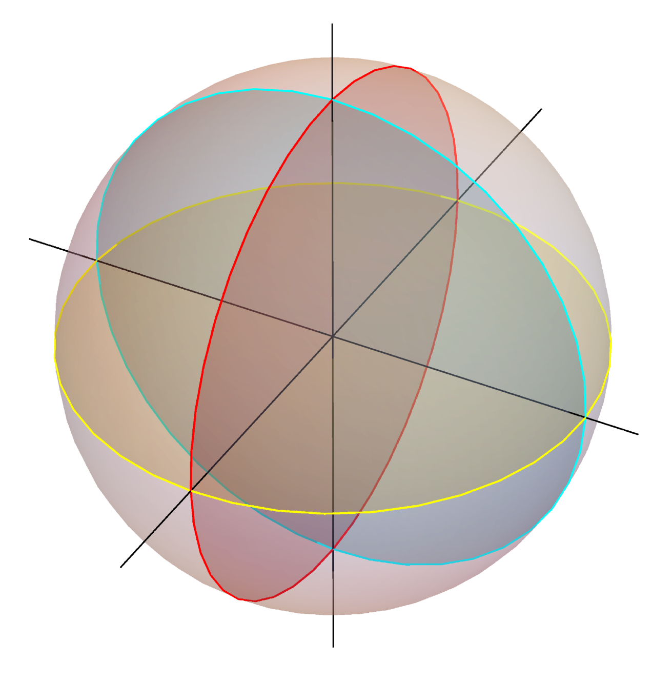
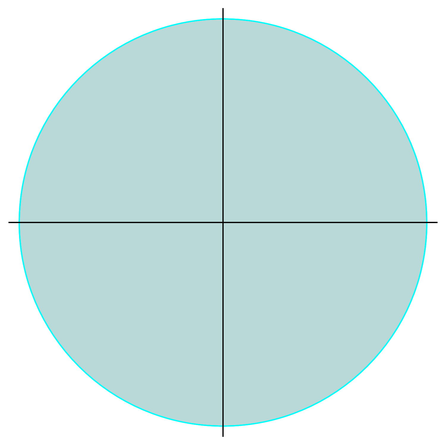
Figure 2: We show the Bloch sphere (a), with $\left|e\right\rangle$ at the “north pole” ($z=1$), and $\left|g\right\rangle$ at the “south pole” ($z=-1$). Any pure qubit state can be represented by a point on the sphere’s surface, while mixed states (i.e. weighted averages of two or more pure–state density operators) live inside the sphere’s surface. In (b), we highlight some of these features in more detail, focusing on the $xz$–plane of the Bloch sphere. Some special states $\left|e\right\rangle={\color[rgb]{1.0,0.22,0.0}\blacktriangle}$, $\left|g\right\rangle={\color[rgb]{0.56,0.0,1.0}\blacktriangledown}$, $\tfrac{1}{\sqrt{2}}(\left|e\right\rangle-\left|g\right\rangle)={\color[rgb]{0.75,0.0,0.2}\blacktriangleleft}$, and $\tfrac{1}{\sqrt{2}}(\left|e\right\rangle+\left|g\right\rangle)={\color[rgb]{1.0,0.08,0.58}\blacktriangleright}$ are marked. A mixed state $\rho_{m}$ is shown as the weighted sum of two pure state density operators $\rho_{\psi}$ and $\rho_{\Upsilon}$(where the vectors drawn are proportional in length to the probability of drawing their respective pure state from an ensemble). We also illustrate the coordinate $\vartheta$ used later in the text.

A qubit is any two–level quantum system; mathematically–speaking this means that it is described like a spin–$\tfrac{1}{2}$. Physically speaking, a qubit might be any of e.g. a particular transition in an atom or ion, a spin in a quantum dot or diamond nitrogen–vacancy center, or the lowest–two levels of the superconducting “artificial atoms” now used in many experiments. The state of a qubit can be represented as living in the Bloch sphere; we will generically parameterize our single–qubit density matrix with Bloch coordinates according to

$$\rho=\frac{1}{2}\left(\begin{array}[]{cc}1+z&x-iy\\ x+iy&1-z\end{array}\right)=\tfrac{1}{2}\left(\openone+x\hat{\sigma}_{x}+y\hat{\sigma}_{y}+z\hat{\sigma}_{z}\right)$$ (1)

throughout the forthcoming derivations, where $(1+z)/2=\rho_{ee}$ denotes the excited state population. See Fig. 2. It is also necessary that we introduce a distinction between pure states, which can be represented by a state vector $\left|\psi\right\rangle$, and mixed states which require the use of $\rho$. Pure qubit states $\rho=\left|\psi\right\rangle\left\langle\psi\right|$ live on the outer surface of the unit sphere, while more general states $\rho=\sum_{i}\wp_{i}\left|\psi_{i}\right\rangle\left\langle\psi_{i}\right|$ may live inside the sphere; a “mixed” state with more than one non–zero $\wp_{i}$ may be used to describe a system which is imperfectly isolated from its surrounding environment, where the $\wp_{i}$ are effectively probabilities. This description implies that we have a ’classical’ statistical mixture, in which we have a probability $\wp_{i}$ of finding the pure state $\left|\psi_{i}\right\rangle$ in an ensemble; in contrast with a coherent pure state superposition, elements in such a mixture do not interfere with each other. For example, we may consider states which lead to a probability $\tfrac{1}{2}$ for a $\sigma_{z}$–measurement to return $\left|e\right\rangle$ or $\left|g\right\rangle$, such as $\left|x+\right\rangle=\tfrac{1}{\sqrt{2}}(\left|e\right\rangle+\left|g\right\rangle)$. The density matrix for this pure state (which contains the possibility for quantum interference) is not the same as the classical statistical mixture of $\left|e\right\rangle$ and $\left|g\right\rangle$ (where the off–diagonal “coherences” are suppressed), i.e.

$$\begin{split}\left|x+\right\rangle\left\langle x+\right|&=\frac{1}{2}\left(\begin{array}[]{cc}1&1\\ 1&1\end{array}\right)\\ &\neq\frac{1}{2}\left(\begin{array}[]{cc}1&0\\ 0&1\end{array}\right)=\tfrac{1}{2}\left|e\right\rangle\left\langle e\right|+\tfrac{1}{2}\left|g\right\rangle\left\langle g\right|.\end{split}$$ (2)

By using the density matrix to describe our state, we may account for all of these options, which is necessary when we have an open system and the possibility of information loss.

Note that $\rho$ is Hermitian ($\rho=\rho^{\dagger}$), and normalization requires that $\text{tr}\left(\rho\right)=1$. We will often represent a qubit’s state and dynamics in terms of the Bloch vector $\mathbf{q}=\{x,y,z\}$ below; such coordinates should be understood in the context of (1). We suppress the “hat” notation on our density operators $\rho$.

II.1 Standard quantum–mechanical treatment

We summarize the typical approach, originally by Weisskopf and Wigner, as a point of departure in describing spontaneous emission. A more complete derivation of the results we summarize can be found in Ref. Jacobs and Steck (2006), and we will stick closely to their conventions for clarity. The Hamiltonian describing the joint system including the qubit and a single mode of the electromagnetic field is of the form

$$\begin{split}\frac{\hat{h}}{\hbar}=&\underbrace{\omega_{\text{qb}}\hat{\sigma}^{+}\hat{\sigma}_{-}}_{\text{qubit}}+\underbrace{\omega_{f}\left(\hat{a}^{\dagger}\hat{a}+\tfrac{1}{2}\right)}_{\text{single field mode}}+\underbrace{\left(g\hat{\sigma}^{+}\hat{a}+g^{\ast}\hat{\sigma}_{-}\hat{a}^{\dagger}\right)}_{\text{interaction }\hat{h}_{int}},\end{split}$$ (3)

where $\hbar\omega_{\text{qb}}$ is the energy separation between the two qubit levels of interest, $\omega_{f}$ denotes the frequency of the field mode, and $g$ is a coupling constant between the field and qubit. The first two terms represent the qubit and field, respectively, while the third term describes their interaction. One can regard this model as corresponding to a two level system and quantum harmonic oscillator which are able to exchange excitations. We have raising and lowering operators on the qubit $\hat{\sigma}^{+}=\left|e\right\rangle\left\langle g\right|$ and $\hat{\sigma}_{-}=\left|g\right\rangle\left\langle e\right|$, and on a field mode $\hat{a}\left|n\right\rangle=\sqrt{n}\left|n-1\right\rangle$ and $\hat{a}^{\dagger}\left|n\right\rangle=\sqrt{n+1}\left|n+1\right\rangle$ for Fock states $\left|n\right\rangle$. The interaction term $\hbar g\hat{\sigma}^{+}\hat{a}$ describes the possibility for the atom to become excited by absorbing a photon (which is removed from the field); the adjoint of this term denotes the reverse process, in which the qubit loses energy, emitting a photon which is added to the field mode. We may use the Schrödinger equation to compute the evolution of the joint system and subsequent qubit state amplitudes under the influence of this Hamiltonian. The electro–magnetic environment of the qubit contains many modes, and the apparently incoherent evolution of the qubit associated with spontaneous emission emerges when summing up the action of the couplings to all these modes, each described like $\hat{h}_{int}$ above. Such analysis requires that we average the evolution predicted by the Schrödinger equation over the available density of free–space field modes and sum over polarizations Jacobs and Steck (2006). To good approximation (i.e. the approximations first made by Weisskopf and Wigner), we may simplify the dynamics at timescales much longer than the field periods, eliminating environmental modes from the description. For a generic qubit state $\zeta\left|e\right\rangle+\phi\left|g\right\rangle$, we obtain the evolution of the excited state amplitude

$$\dot{\zeta}=\left(-i\omega_{\text{qb}}-\tfrac{\gamma}{2}\right)\zeta.$$ (4)

We have introduced the spontaneous emission rate $\gamma=T_{1}^{-1}$ which is equal to the density of modes coupled resonantly to the qubit via $\gamma=\sum_{j}|g_{j}|^{2}\delta(\omega_{\text{qb}}-\omega_{j})$. Here, $g_{j}$ stands for the strength of the coupling to the $j^{\text{th}}$ mode of the electromagnetic reservoir. The contributions of all the non–resonant modes oscillate and quickly average to zero over a typical time $\tau_{\text{corr}}\ll\gamma^{-1}$; this condition is key in allowing us to obtain a Markovian description of the qubit evolution (4), from which the reservoir dynamics have been completely eliminated. A precise discussion of the approximations leading to Eq. (4) and the order of the associated errors can be found in Ref. Cohen-Tannoudji et al. (1998), Chapter 4.

The excited state population is described by the density matrix element

$$\rho_{ee}=\zeta^{\ast}\zeta=(z+1)/2.$$ (5)

It is straightforward to compute that (4) and (5) imply

$$\dot{\rho}_{ee}=-\gamma\rho_{ee}\quad\leftrightarrow\quad\dot{z}=-\gamma\left(z+1\right).$$ (6)

The result that spontaneous emission leads to exponential decay of the excited state population at rate $\gamma$ (or with characteristic time $T_{1}=\gamma^{-1}$), absent other dynamics, is among the most fundamental phenomena in the quantum optics literature.

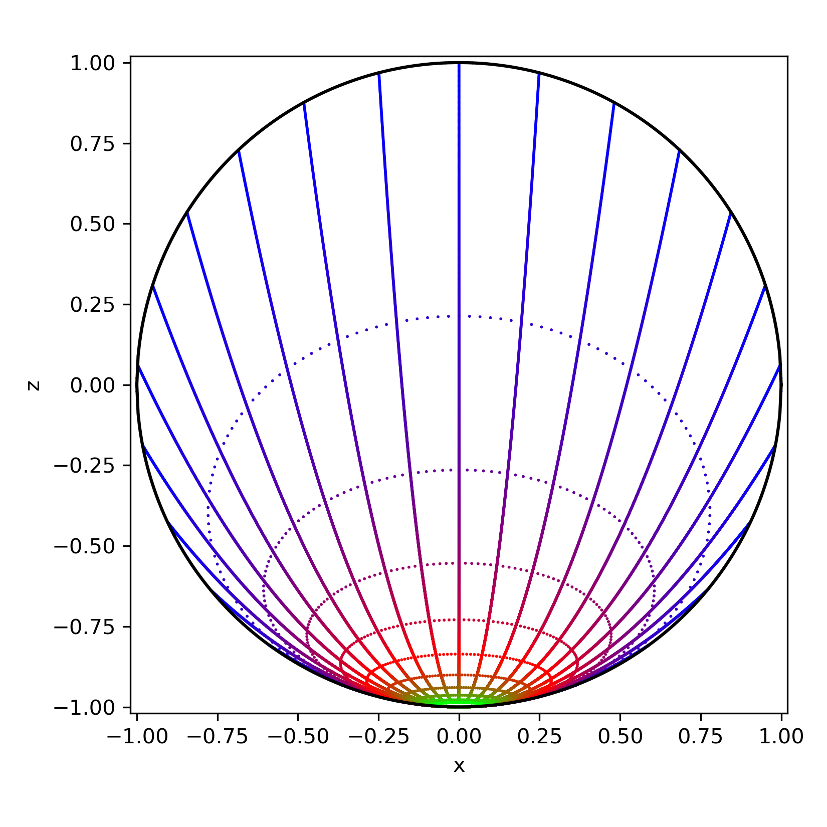
Figure 3: We plot the evolution of the qubit state under the unmonitored fluorescence dynamics (10) in the $xz$–plane of the Bloch sphere, originating from a variety of initial pure states. The excited state is at the top of the sphere, and all paths converge towards the ground state at the bottom. Color denotes the time evolution along each path. The trajectories in the qubit state tend to become impure / mixed, because no information is collected about fluorescence output; we have an open system with lost information in this case. These dynamics are often represented with an equivalent picture in which the Bloch ball contracts into an ellipsoid near the ground state under the influence of a decay channel Nielsen and Chuang (2000); we sample a greater number of initial states at intervals of $T_{1}/2$ to illustrate this.

II.2 Master equation treatment

In order to express the complete information about the qubit state at any time in a compact way, and straightforwardly generalize our system (e.g. we might consider coherently driving qubit), it is convenient to formulate the dynamics of spontaneous emission as a master equation for the density operator $\rho$ introduced above. The evolution of an open quantum system in contact with a Markovian environment (i.e. with an environment of very short correlation time $\tau_{\text{corr}}$ with respect to the other time scales in the problem) can, in general, be written as a Lindblad equation; such a master equation is of the form Haroche and Raimond (2006)

$$\dot{\rho}=\underbrace{\frac{i}{\hbar}[\rho,\hat{H}]}_{\text{Unitary Evol.}}+\underbrace{\sum_{c}\left(\hat{L}_{c}\rho\hat{L}_{c}^{\dagger}-\tfrac{1}{2}\hat{L}_{c}^{\dagger}\hat{L}_{c}\rho-\tfrac{1}{2}\rho\hat{L}_{c}^{\dagger}\hat{L}_{c}\right)}_{\text{Lindblad Dissipation}},$$ (7)

where $\rho$ is the density matrix of the system of primary interest (in this case, the qubit), and each operator $\hat{L}_{c}$ describes a coupling between the system and its environment (in this case, the decay channel). We see a term describing the unitary evolution $\dot{\rho}=\tfrac{i}{\hbar}[\rho,\hat{H}]$, plus the Lindblad term which accounts for information leaking into the environment through any channels to which the system is open.

The arguments of the previous section can be used to show that the case of spontaneous emission corresponds to a single channel characterized by operator $\hat{L}=\sqrt{\gamma}\hat{\sigma}_{-}$ Cohen-Tannoudji et al. (1998), which indicates that the qubit may lose its excitation with an effective coupling rate $\gamma$. The master equation capturing spontaneous emission of a qubit is then

$$\dot{\rho}=\frac{i}{\hbar}[\rho,\hat{H}]+\gamma\hat{\sigma}_{-}\rho\hat{\sigma}^{+}-\tfrac{\gamma}{2}\left(\hat{\sigma}^{+}\hat{\sigma}_{-}\rho+\rho\hat{\sigma}^{+}\hat{\sigma}_{-}\right),$$ (8)

where the qubit Hamiltonian is $\hat{H}=\hbar\omega_{\text{qb}}\hat{\sigma}_{z}/2$. The unitary part solely induces a rotation at frequency $\omega_{\text{qb}}$ of the qubit state around the $z$-axis of the Bloch sphere, and it is convenient to work in a frame in which this rotation is suppressed. This rotating frame is formally the interaction picture with respect to $\hat{H}$, associated with the transformation $\rho\to e^{i\hat{H}t/\hbar}\rho e^{-i\hat{H}t/\hbar}$. In the following, we will always work in such frame, where the master equation reads

$$\dot{\rho}=\gamma\hat{\sigma}_{-}\rho\hat{\sigma}^{+}-\tfrac{\gamma}{2}\left(\hat{\sigma}^{+}\hat{\sigma}_{-}\rho+\rho\hat{\sigma}^{+}\hat{\sigma}_{-}\right).$$ (9)

We can get equations of motion in the Bloch coordinates (in the rotating frame) by computing $\dot{\mathbf{q}}=\text{tr}(\hat{\sigma}_{\mathbf{q}}\dot{\rho})$, yielding

$$\dot{x}=-\frac{\gamma}{2}x,\quad\dot{y}=-\frac{\gamma}{2}y,\quad\dot{z}=-\gamma(1+z),$$ (10)

in perfect agreement with the treatment above (6). The decaying solutions of these equations, initialized from different pure states on the edge of the Bloch sphere, are illustrated in Fig. 3.

For many application, the qubit needs to be driven; to describe such a situation, we must modify the qubit Hamiltonian $\hat{H}$, adding time–dependent terms. In general, the derivation of the master equation describing the dynamics of the qubit’s density operator needs to be carefully redone in presence of this new Hamiltonian, and one may find that the Lindblad term is modified due to the presence of the drive Breuer and Petruccione (2002). Such a modification typically occurs, for example, when the drive causes the qubit to become sensitive to modes of the environment at different frequencies, which are sufficiently separated from each other so as to have a different density of states. For instance, in the case of a quasi–resonant monochromatic drive inducing Rabi oscillations, the emission spectrum of the qubit contains multiple peaks (the famous Mollow triplet Mollow (1969)) separated by the Rabi frequency (which is related to the intensity of the driving). If the environmental density of state varies around the qubit frequency $\omega_{\text{qb}}$ on the Rabi frequency scale, the form of the damping is drastically modified. In Ref. Murch et al. (2012) this effect was exploited to stabilize an arbitrary state of the Bloch sphere. However, provided the drives are weak enough (Rabi frequencies much smaller than the qubit frequency and the inverse correlation time of the reservoir $\tau_{\text{corr}}$), and there is no cavity or other resonance close to the driven qubit’s emission spectrum peaks to cause especially fast variations in the environment spectrum Carmichael (1999), this effect is negligible. Within these conditions, the action of a drive can be simply captured by adding a unitary term $(i/\hbar)[\rho,\hat{H}_{\text{dr}}(t)]$ in Eq. (8); the treatment we develop below assumes this simplest case. While some modification to this simplest scheme may be necessary in adapting it to situations beyond the stated constraints, experiments not explicitly focused on engineering more exotic effects will typically obey these simplifying constraints by default; this simplest scheme we lay out below is thus widely applicable.

III Quantum Trajectories

The treatment of spontaneous emission in the previous section, and in particular the master equation Eq. (9), captures the dynamics of the qubit under the assumption that any information emitted by the qubit (leaking into the environment) during the qubit-field mode interaction is lost forever. We are, however, primarily interested in the case where we, the observer(s), recover some (or ideally all) of this information through measurement(s) on the field mode. In this section, we present the formalism of Kraus operators, which describes the update of the qubit’s state conditioned on acquiring such information.

III.1 Kraus Operator Formalism

The basic idea is that there exist a set of Kraus operators $\hat{M}_{r}$, which describe how the state of our system should be updated, each of them conditioned on acquiring one of the possible measurement outcomes $r$ in the environment during a measurement of duration $dt$, according to Nielsen and Chuang (2000); Wiseman and Milburn (2010); Haroche and Raimond (2006)

$$\rho(t+dt)=\frac{\hat{M}_{r}\rho(t)\hat{M}_{r}^{\dagger}}{\text{tr}\left(\hat{M}_{r}\rho(t)\hat{M}_{r}^{\dagger}\right)}.$$ (11)

We require that either $\sum_{r}\hat{M}_{r}^{\dagger}\hat{M}_{r}=\openone$, or $\int dr\hat{M}_{r}^{\dagger}\hat{M}_{r}=\openone$, depending on whether the possible measurement outcomes $r$ are discrete or continuous; such a condition tells us that we have a valid (completely positive) transformation on $\rho$, and insures that we have considered a complete, self–consistent set of measurement outcomes. As dictated by the axioms of quantum mechanics, the outcome $r$ is obtained randomly among its possible values based on Born’s rule, which here yields probabilities (or a probability density) $\wp(r|\rho)=\text{tr}\left(\hat{M}_{r}\rho\hat{M}_{r}^{\dagger}\right)$. Note that the denominator of (11), which serves to ensure the updated density matrix is properly normalized, exactly matches this probability. If measurement(s) on the environment is(are) repeated (in our case every $dt$), the successive outcomes and subsequent state updates define a stochastic sequence of states called a quantum trajectory.

Following Ref. Jordan et al. (2015), we construct the particular $\hat{M}$ of interest for the case of a spontaneously–emitting qubit, using a Bayesian probability argument; it is useful to consider a pure state of the qubit and an effective field mode it emits into (initially in vacuum state $\left|0\right\rangle$)

$$\left|\psi_{0}\right\rangle=\left(\zeta\left|e\right\rangle+\phi\left|g\right\rangle\right)\otimes\left|0\right\rangle,$$ (12)

where $z=2|\zeta|^{2}-1$, and $\left|e\right\rangle$ and $\left|g\right\rangle$ are the excited and ground states of the qubit, respectively. There is a probability $\wp(e)=|\zeta|^{2}$ to find the qubit in $\left|e\right\rangle$ and probability $\wp(g)=|\phi|^{2}$ to find the qubit in $\left|g\right\rangle$, with $\wp(e)+\wp(g)=1$. On phenomenological grounds, we suppose that the probability for an emission event in a time interval $dt$ is given by $\wp(1|e)=\epsilon=\gamma\>dt$, where $\gamma$ is some characteristic rate at which the qubit fluoresces (i.e. $\gamma=1/T_{1}$ is a measurable quantity for a qubit–cavity system). Then $\wp(1|e)\wp(e)=\epsilon|\zeta|^{2}=\wp(e|1)\wp(1)$ and/or $\wp(0|e)\wp(e)=(1-\epsilon)|\zeta|^{2}=\wp(e|0)\wp(0)$ according to Bayes’ theorem. A quantum–coherent state assignment after the short interval $dt$ which reflects these probabilistic considerations is

$$\left|\psi_{1}\right\rangle=\sqrt{1-\epsilon}\zeta\left|e,0\right\rangle+\phi\left|g,0\right\rangle+\sqrt{\epsilon}\zeta\left|g,1\right\rangle.$$ (13)

In other words, there is some probability for an emission event which involves a photon being created in the output mode ($0\rightarrow 1$), and which shifts qubit population from $\left|e\right\rangle\rightarrow\left|g\right\rangle$, reflecting a common sense understanding of spontaneous emission. Below we will always assume that the measurement time (in practice, a detector integration time) is much faster than the characteristic decay time of the qubit, i.e. we have $dt\ll T_{1}$, or $\epsilon\ll 1$. This is a key condition which will ensure that the quadrature measurements we will eventually consider are weak measurements, and that the subsequent quantum trajectories are diffusive. We also assume that the information we acquire applies to the qubit in real time, which implies that that photon travel time between the qubit and measurement apparatus should be negligible. We may rewrite the change of state from above as

$$\left|\psi_{1}\right\rangle=\left(\begin{array}[]{cc}\sqrt{1-\epsilon}&0\\ \sqrt{\epsilon}\hat{a}^{\dagger}&1\end{array}\right)\left|\psi_{0}\right\rangle\text{ for }\left|\psi_{0}\right\rangle=\left(\begin{array}[]{c}\zeta\\ \phi\end{array}\right)\otimes\left|0\right\rangle,$$ (14)

where $a^{\dagger}$ creates a photon in the relevant cavity/field output ($a^{\dagger}\left|0\right\rangle=\left|1\right\rangle$). The Kraus operators $\hat{M}_{\text{r}}$ in (11) act only on the qubit state, and are obtained by projecting out the field mode in a final state corresponding to some outcome from measuring the field, i.e.

$$\hat{M}_{r}=\left\langle\psi_{r}\right|\left(\begin{array}[]{cc}\sqrt{1-\epsilon}&0\\ \sqrt{\epsilon}\hat{a}^{\dagger}&1\end{array}\right)\left|0\right\rangle,$$ (15)

where $\{\left|\psi_{r}\right\rangle\}$ could be any basis of states of the field mode, which should be chosen based on the kind of measurement being performed and result $r$. All of the examples we consider below rely on a Kraus operator of the form (15). Much of what we do below will revolve around relating different measurements to the appropriate choice of $\left|\psi_{r}\right\rangle$, and then exploring the ramifications that choice has on the measurement backaction and quantum trajectories.

III.2 Photodetection and quantum jump trajectories

As a first example, suppose that we choose our $\left|\psi_{r}\right\rangle$ in the Fock basis, i.e. we consider outcomes of the type $\left|1\right\rangle$ (a photon exits in the field mode in the given timestep), or $\left|0\right\rangle$ (no photon exits), which correspond to making a photodetection measurement. In other words, we imagine counting the photons emitted by the qubit into the field mode, in a time–resolved manner, with a detector integration time $dt\ll\gamma^{-1}$ (equivalently, $\epsilon\ll 1$).

We may define Kraus operators $\hat{M}_{1}$ ($\hat{M}_{0}$) for the single–qubit state update conditioned on a click (no–click) in the detector, according to

$$\hat{M}_{0}=\left\langle 0\right|\left(\begin{array}[]{cc}\sqrt{1-\epsilon}&0\\ \sqrt{\epsilon}\hat{a}^{\dagger}&1\end{array}\right)\left|0\right\rangle=\left(\begin{array}[]{cc}\sqrt{1-\epsilon}&0\\ 0&1\end{array}\right),$$ (16)

$$\hat{M}_{1}=\left\langle 1\right|\left(\begin{array}[]{cc}\sqrt{1-\epsilon}&0\\ \sqrt{\epsilon}\hat{a}^{\dagger}&1\end{array}\right)\left|0\right\rangle=\left(\begin{array}[]{cc}0&0\\ \sqrt{\epsilon}&0\end{array}\right).$$ (17)

It is easy to verify that $\hat{M}_{0}^{\dagger}\hat{M}_{0}+\hat{M}_{1}^{\dagger}\hat{M}_{1}=\openone$, such that these measurement operators form a positive operator valued measure (POVM) Nielsen and Chuang (2000). We can say that under continuous photodetection, the qubit state is updated every $dt$ by

$$\rho(t+dt)=\frac{\hat{M}_{1}\rho(t)\hat{M}_{1}^{\dagger}}{\text{tr}\left(\hat{M}_{1}\rho(t)\hat{M}_{1}^{\dagger}\right)},$$ (18)

if the detector registers that a photon emerged between $t$ and $t+dt$, or according to

$$\rho(t+dt)=\frac{\hat{M}_{0}\rho(t)\hat{M}_{0}^{\dagger}}{\text{tr}\left(\hat{M}_{0}\rho(t)\hat{M}_{0}^{\dagger}\right)}$$ (19)

if no photon reaches the detector. The probability of a click in any given timestep is $\wp_{1}=\text{tr}(\hat{M}_{1}\rho(t)\hat{M}_{1}^{\dagger})=\gamma\>dt\>(1+z)/2$, and the probability of no–click is $\wp_{0}=\text{tr}(\hat{M}_{0}\rho(t)\hat{M}_{0}^{\dagger})$, with $\wp_{0}+\wp_{1}=1$. These expressions reflect the common–sense result that $\wp_{1}$ must vanish when the qubit is in the ground state, i.e. $\wp_{1}=0$ for $z=-1$. Thus, a single quantum trajectory for this photodetection scenario is characterized by a time series of outcomes $r\in\{0,1\}$. Simulation of such a trajectory can be performed by drawing a click/no–click readout from a binomial distribution at each short timestep of duration $dt\ll T_{1}$, and subsequently updating the qubit state $\rho$ according to the appropriate rule above. Results of such a simulation are shown in Fig. 5(a). The trajectories generated by photodetection are an example of “quantum jump” trajectories, for which the qubit state immediately jumps to $\left|g\right\rangle$ when a click event occurs (this is related to the discrete nature of the possible outcomes $r$).

Before moving on to different types of measurements on the output mode, we bridge the gap between our Kraus operator description and the un-monitored decay channel we discussed in the previous section. The situation in which the outcome of the measurement performed on the field mode between $t$ and $t+dt$ is actually unavailable can be captured by averaging the state update over both outcomes, i.e.

$$\rho(t+dt)=\frac{\hat{M}_{0}\rho(t)\hat{M}_{0}^{\dagger}+\hat{M}_{1}\rho(t)\hat{M}_{1}^{\dagger}}{\text{tr}\left(\hat{M}_{0}\rho(t)\hat{M}_{0}^{\dagger}+\hat{M}_{1}\rho(t)\hat{M}_{1}^{\dagger}\right)}.$$ (20)

An equation of motion can be obtained by taking

$$\dot{\rho}\approx\frac{\rho(t+dt)-\rho(t)}{dt},$$ (21)

where the numerator on the RHS is expanded to $O(dt)$. It is then straightforward to verify that the equations (10) reappear exactly, i.e. the procedure just described to obtain $\dot{\rho}$ leads to exactly the same expression as the master equation as described above, and as shown in Fig. 3. A similar procedure allows to show that for any measurement basis $\left|\psi_{r}\right\rangle$ chosen for the field, the master equation is recovered when averaging over all of the outcomes we could have obtained from measurement; we will soon be able to elaborate further on this point.

III.3 Diffusive trajectories and stochastic master equation

In the remainder of this article, we are concerned about measurements on the environment leading to a continuous–valued outcome $r$, e.g. a voltage or current from a detector, leading to “diffusive” trajectories (in contrast with the “jump” trajectories we have just discussed). The specifics of the two most common examples, heterodyne and homodyne measurements, are presented in detail in the following section. Because the evolution during $dt$ is infinitesimal, it is common to write the change in the density operator of the qubit, conditionned on the outcome $r$ obtained at time $t$, under the form of a stochastic master equation (SME); the SME can be seen as an extension of Eq. (7), in which we add a term which accounts for the measurement outcome. The SME may generically be obtained by expanding an expression of the form (11) to $O(dt)$ Brun (2002); Jacobs and Steck (2006) (detailed examples of this process follow below). The addition of a stochastic element into a differential equation is not trivial, because a genuinely stochastic element is not really differentiable, the way a smooth and well–behaved function is.

Generically, what we will momentarily consider is a type of Langevin equation, or first–order stochastic differential equation of the form

$$\dot{q}=\mathsf{a}(q)+\mathsf{b}(q)\xi(t);$$ (22)

the term $\mathsf{a}$ is often called the drift term, whereas $\mathsf{b}$ functions as a diffusion constant, and together with the randomly–varying $\xi(t)$, gives stochastic evolution. Equations of this type were first written down to model Brownian motion of small particles Feynman , where complex mechanical forces lead to effectively random kicks in a particle’s position. In our present case, we care about the evolution of a quantum state, and the stochasticity denoted by $\xi(t)$ is a result of the randomness inherent in the quantum measurement process. The particular type of random evolution we consider is delta–correlated Gaussian white noise, obeying $\xi(t)=dW(t)/dt$, where $W(t)$ is called a Wiener process. The Wiener increment $dW(t)=W(t+dt)-W(t)$ is a Gaussian random variable, independent on any past values $dW(s)$ for $s<t$ and characterized by a mean of zero and variance equal to $dt$. These properties lead to a noise term $\xi(t)$ of zero expectation value $\langle\langle\xi(t)\rangle\rangle=0$ and co-variance obeying $\langle\langle\xi(t)\xi(t^{\prime})\rangle\rangle=\delta(t-t^{\prime})$, where the double bracket indicates the ensemble average over realizations of the process. This is suitable for describing the quantum noise arising from measurement in a variety of physical situations, including those we consider below. Some physical justification for the appropriateness of the use of a Gaussian $\xi$ for the examples below is provided in the following sections, and in Appendix A. For $\mathsf{a}=0$ and constant $\mathsf{b}$ (simple diffusion without drift), the variance of an ensemble of diffusing trajectories scales like time; this is summarized by the Itô stochastic calculus rule $dW(t)^{2}=dt$ (or equivalently $\xi(t)^{2}=1/dt$).

The general form of the SME that we use for diffusive quantum trajectories, in units $\hbar\rightarrow 1$, reads Jacobs and Steck (2006); Wiseman and Milburn (2010)

$$d\rho=i[\rho,\hat{H}]dt+\sum_{c}\left(\hat{\mathcal{L}}[\rho,\hat{L}_{c}]dt+\sqrt{\eta_{c}}\hat{\mathcal{M}}[\rho,\hat{L}_{c}]dW_{c}\right).$$ (23)

The super–operators are the Lindblad dissipation term, from (7),

$$\hat{\mathcal{L}}[\rho,\hat{L}_{c}]\equiv\hat{L}_{c}\rho\hat{L}_{c}^{\dagger}-\tfrac{1}{2}\left(\hat{L}_{c}^{\dagger}\hat{L}_{c}\rho+\rho\hat{L}_{c}^{\dagger}\hat{L}_{c}\right),$$ (24)

and the newly–added measurement backaction term

$$\hat{\mathcal{M}}[\rho,\hat{L}_{c}]\equiv\hat{L}_{c}\rho+\rho\hat{L}_{c}^{\dagger}-\rho\>\text{tr}\left(\hat{L}_{c}\rho+\rho\hat{L}_{c}^{\dagger}\right).$$ (25)

As before, a Hamiltonian $\hat{H}$ may describe any unitary processes applied to the system (e.g. Rabi drive on a qubit). Each of the operators $\hat{L}_{c}$ describes a particular measurement channel, which is monitored with efficiency $\eta_{c}\in[0,1]$ (where $1$ denotes perfect measurement efficiency, and $\eta_{c}$ is dimensionless). The measurement record associated with any monitored channel, contains one outcome every $dt$, going like $r_{c}\propto\sqrt{\eta_{c}}\langle\hat{L}_{c}+\hat{L}_{c}^{\dagger}\rangle+\xi_{c}$, where the brackets denote the expectation value in state $\rho$. Such an expression for the readout is easy to interpret as a signal $\langle\hat{L}_{c}+\hat{L}_{c}^{\dagger}\rangle$, attenuated due to inefficiency by a factor $\sqrt{\eta_{c}}$, plus quantum noise $\xi_{c}$ intrinsic to the measurement process. A more detailed introductory guide to SME can be found in Ref. Jacobs and Steck (2006).

Channels which are open to the environment, but un-monitored (e.g. typical dephasing mechanisms, or the decay channel in the un-monitored case), can be modeled by placing an operator in the sum over $c$ which is monitored with efficiency $\eta_{c}=0$. The master equation (7) can be recovered from the SME by taking an ensemble average over stochastic trajectories Applying these concepts to the example of a single decay channel introduced above, we see that 1) opening the qubit to an unmonitored decay channel $\hat{L}=\sqrt{\gamma}\hat{\sigma}_{-}$, 2) measuring the qubit fluorescence/decay according to $\hat{L}=\sqrt{\gamma}\hat{\sigma}_{-}$ with efficiency zero, or 3) the average dynamics over an ensemble of stochastic trajectories obtained by continuously monitoring the qubit fluorescence as per $\hat{L}=\sqrt{\gamma}\hat{\sigma}_{-}$, are all equivalent situations. This view from the master equation is also entirely equivalent to that for the Kraus operators, as presented in and around (20). In Fig. 5 we observe this in simulations, observing that the average over many quantum trajectories reproduces the dynamics of the unmonitored case (10), regardless of the character of the individual measurements.

Figure 4: We illustrate some of the concepts implicit in (26). The Itô–like choice $\beta=0$ is illustrated with red boxes in all subfigures, while the Stratonovich–like choice $\beta=\tfrac{1}{2}$ is illustrated with the blue trapezoids in all subfigures. We see these applied to an ordinary differential equation ($\mathsf{b}=0$) on the left, and to a stochastic differential equation ($\mathsf{b}\neq 0$) on the right, with timesteps decreasing as we go from the top down. All choices of $\beta$ will converge to the same area under the curve in the time–continuum limit for smooth function on the left. For the stochastic process depicted on the right, however, (which remains stochastic at any timescale, such that the kind of picture on the left never emerges from it), different choices of $\beta$ will not necessarily lead to the same solution. Some ramifications of this are discussed in the main text, leading to equations (27) through (29).

In the sections below, we will formallly compare equations of motion derived from our Kraus operator methods to those from the SME; in order to do this, it is necessary that we briefly comment on a technical issue pertaining to stochastic calculus and the integration of stochastic differential equations. The calculus used to derive and/or manipulate a Langevin of the type above is closely tied to the type of Riemann sum used as the basis of any subsequent integration. If we were integrating an ordinary differential equation, any valid choice of Riemann sum would lead to the same result in the time–continuum limit. This is not so in the stochastic case however; if we suppose that $dW$ is stochastic at every time–scale, different Riemann sums will not converge to the same solutions in the limit anymore! To get the idea, we may consider a discrete update step

$$q_{k+1}-q_{k}=\mathsf{a}(\tilde{q}_{k})\Delta t+\mathsf{b}(\tilde{q}_{k})\Delta W_{k},$$ (26)

where we have $\tilde{q}_{k}=\beta q_{k+1}+(1-\beta)q_{k}$, and the indices $k$, $k+1$ correspond to times $\Delta t$ apart. We highlight two very common conventions: The Itô convention uses $\beta=0$, such that we evaluate drift and diffusion coefficients at the beginning of a timestep, whereas the Stratonovich convention corresponds to $\beta=\tfrac{1}{2}$, such that functions are evaluated according to a trapezoidal rule (see Fig. 4). The form of the SME (23) assumes a derivation based on Itô calculus, in which expansions are made to $O(dt)$ using the rule $dW^{2}=dt$ (i.e. expansions to $O(dt)$ must include explicit expansions to $O(dW^{2})$ in that formalism Jacobs and Steck (2006)). For an accessible and intuitive explanation of this rule, we encourage the interested reader to look at section 4 of Ref. Gough (2018a). Expansions made with regular calculus will lead a Stratonovich equation instead however. In other words, we have to consider two different stochastic calculus conventions, each leading to different differential equations; they give consistent results, however, when paired with the correct integration rules. Specifically: Integrating the equation

$$d\mathbf{q}=\mathbf{a}(\mathbf{q})\>dt+\mathbf{b}(\mathbf{q})\>d\bm{W}$$ (27)

according to the Itô sense ($\beta=0$), is equivalent to performing a Stratonovich integration ($\beta=\tfrac{1}{2}$) on

$$\dot{\mathbf{q}}=\mathbf{A}(\mathbf{q})+\mathbf{b}(\mathbf{q})\>\bm{\xi},$$ (28)

where the two drift terms $\mathbf{a}$ and $\mathbf{A}$ are related by the transformation

$$A_{q}=a_{q}-\tfrac{1}{2}\sum_{j,n}b_{jn}\partial_{n}b_{jq};$$ (29)

$n$ indexes the coordinates (components of $\mathbf{q}$), and $j$ indexes the independent noise(s) on each measurement channel, which are summed. For justification and details see e.g. Gardiner (2004); Kloeden and Platen (1992). We will use this conversion rule to connect different descriptions of the quantum measurement scenarios we consider below.

We make a final remark about numerical simulations before moving on. The appeal of the SME as a theoretical tool is that it expresses quantum trajectory dynamics as a differential equation, similar to how physicists are accustomed to describing classical dynamics; furthermore, the SME readily splits those dynamics into three terms, which make qualitatively distinct contributions to the dynamics. It is worth noting, however, that compared with the case of ordinary differential equations Press et al. (1988), methods for the numerical integration of stochastic differential equations Kloeden and Platen (1992) are more complex, and are accurate only to substantially lower order in $dt$. Additionally, direct numerical integration of the SME does not necessarily preserve the properties of a valid density matrix beyond $O(dt)$, leading to problematic numerical errors unless $dt$ is extremely small; it is consequently numerically preferable to execute simulations of stochastic quantum trajectories by direct application of a positive mapping, as in (11) or similar, when possible. The interested reader may find further comments in this vein e.g. in Ref. Rouchon and Ralph (2015).

IV Single–Qubit Heterodyne Trajectories

We now begin looking at diffusive quantum trajectories due to heterodyne detection. What follows is essentially a review of the simplest non–trivial case described more extensively in Ref. Jordan et al. (2015), and corresponding to the experimental implementation e.g. of Ref. Campagne-Ibarcq et al. (2016a). In the language of quantum–limited amplifiers (QLAs), which are essential to realizing experiments involving individual quantum trajectories, our meaning of “heterodyne” corresponds to “phase–preserving” amplification (e.g. see Clerk et al. (2010); Bergeal et al. (2010); Emmanuel Flurin (2014); Roy and Devoret (2016) or similar, regarding implementations in circuit QED scenarios). See Fig. 1. Owing to the mixing of the fluorescence signal with a coherent state of the field (the “local oscillator”, or LO), the heterodyne measurement gives access to both quadratures of the field, with a symmetric uncertainty. A reader unfamiliar with a quadrature phase space representation of a field mode may benefit from perusing e.g. Ref. Silberhorn (2007). When performed with an ideal QLA, this scheme is formally equivalent to projecting the field mode into the basis of the coherent states Jordan et al. (2015).

IV.1 Stochastic Master Equation Treatment

The SME is given in Eq. (23), and provides one of the most–used approaches to modeling diffusive quantum trajectories arising from continuous weak measurement Brun (2002); Jacobs and Steck (2006). We will consider an idealized measurement in the rotating frame, characterized by $\hat{H}=0$ (no unitary dynamics), $\hat{L}_{X}=\hat{\sigma}_{-}\sqrt{\gamma/2}$, and $\hat{L}_{P}=i\hat{\sigma}_{-}\sqrt{\gamma/2}$, where there is no dephasing channel and the measurement efficiency $\eta=1$ is perfect. We can make qualitative sense of the two operators $\hat{L}_{X}$ and $\hat{L}_{P}$ by understanding that $\hat{\sigma}_{-}$ indicates that our measurement is being made through a decay channel, and that $\hat{L}_{X}$ and $\hat{L}_{P}$ are associated, respectively, with the information encoded in the two quadratures $\hat{X}$ and $\hat{P}$ of the field read out by the heterodyne measurement; the factor $i$ between $\hat{L}_{X}$ and $\hat{L}_{P}$ is the $90^{\circ}$ phase between these two orthogonal directions in the $XP$–plane (often also conventially labeled as the $IQ$–plane).

The resulting SME is then

$$\dot{\rho}=\hat{\mathcal{L}}[\rho,\hat{L}_{X}]+\hat{\mathcal{L}}[\rho,\hat{L}_{P}]+\hat{\mathcal{M}}[\rho,\hat{L}_{X}]\xi_{X}+\hat{\mathcal{M}}[\rho,\hat{L}_{P}]\xi_{P},$$ (30)

where $\hat{\mathcal{L}}$ and $\hat{\mathcal{M}}$ are still the Lindblad dissipation, and measurement backaction terms, respectively. The Gaussian white noise for the measurement channels is characterized by each $\xi(t)\sim dW/dt$. We may obtain equations of motion in terms of Bloch sphere coordinates using $\dot{\mathbf{q}}=\text{tr}(\hat{\sigma}_{\mathbf{q}}\>\dot{\rho})$, yielding

$$\dot{x}=-\tfrac{\gamma}{2}x+\sqrt{\tfrac{\gamma}{2}}\left[\left(1+z-x^{2}\right)\xi_{X}-x\>y\>\xi_{P}\right],$$ (31a)

$$\dot{y}=-\tfrac{\gamma}{2}y+\sqrt{\tfrac{\gamma}{2}}\left[\left(1+z-y^{2}\right)\xi_{X}-x\>y\>\xi_{P}\right],$$ (31b)

$$\dot{z}=-\gamma(1+z)-\sqrt{\tfrac{\gamma}{2}}(1+z)\left[x\>\xi_{X}+y\>\xi_{P}\right],$$ (31c)

in agreement with the result in eq. (25) of Jordan et al. (2015) (for $u=1+z$, $\eta=1$, and $\gamma_{\phi}=0$, in their notation). The stochastic readouts (signals arising from the measurement process) are given by

$$r_{X}=\langle\hat{L}_{X}+\hat{L}_{X}^{\dagger}\rangle+\xi_{X}=\sqrt{\tfrac{\gamma}{2}}x+\xi_{X},$$ (32a)

$$r_{P}=\langle\hat{L}_{P}+\hat{L}_{P}^{\dagger}\rangle+\xi_{P}=\sqrt{\tfrac{\gamma}{2}}y+\xi_{P}.$$ (32b)

Notice that the average path given by these equations (where averages over an ensemble lead to $\xi\rightarrow 0$, since these are zero–mean stochastic variables) obeys the same basic fluorescence relations (10). This is a typical example of the relationship between an un-monitored and continuously–monitored system, as we have discussed in general above.

We will interpret the equations (31) as being equations suitable for Itô integration and stochastic calculus (consistent with the assumptions used to derive (23) in the first place Jacobs and Steck (2006)). It will also be useful to have the corresponding Stratonovich version of this system of equations, which can be manipulated using regular calculus. In this case, the conversion (29) can be written as

$$\mathbf{A}=\mathbf{a}-\tfrac{1}{2}(\mathbf{b}_{X}\cdot\nabla)\mathbf{b}_{X}-\tfrac{1}{2}(\mathbf{b}_{P}\cdot\nabla)\mathbf{b}_{P};$$ (33)

a trio of Stratonovich equations corresponding to the Itô equations (31) are obtained by substituting this new drift vector (33) into (28).

IV.2 Kraus Operator Treatment

We now consider the corresponding Kraus operator treatment of this situation. As discussed previously, a heterodyne measurement effectively projects the fluorescence signal onto a coherent state (77) at each measurement timestep, such that we write down an operator

$$\hat{M}_{\alpha}=\left\langle\alpha\right|\left(\begin{array}[]{cc}\sqrt{1-\epsilon}&0\\ \sqrt{\epsilon}\hat{a}^{\dagger}&1\end{array}\right)\left|0\right\rangle=e^{-|\alpha|^{2}/2}\left(\begin{array}[]{cc}\sqrt{1-\epsilon}&0\\ \sqrt{\epsilon}\alpha^{\ast}&1\end{array}\right).$$ (34)

We will use a substitution for the readouts given by

$$\alpha=\sqrt{\frac{dt}{2}}(r_{X}-ir_{P});$$ (35)

the prefactor $\sqrt{dt/2}$ is chosen because it generates statistics consistent with the shot–noise of the coherent state LO; for clarification see Jordan et al. (2015) and/or appendix A. With this substitution, we have a Kraus operator

$$\begin{split}\hat{M}_{\alpha}&=\exp\left[-\tfrac{dt}{4}(r_{X}^{2}+r_{P}^{2})\right]\left(\begin{array}[]{cc}\sqrt{1-\gamma\>dt}&0\\ \sqrt{\tfrac{\gamma}{2}}dt(r_{X}+ir_{P})&1\end{array}\right),\end{split}$$ (36)

which may be used to update the state (using (11) with $\hat{M}_{r}\rightarrow\hat{M}_{\alpha}$) conditioned on acquiring a measurement record drawn from the probability density $\wp(r_{X},r_{P}|\rho(t))=\mathcal{N}\text{tr}\left(\hat{M}_{\alpha}\rho(t)\hat{M}_{\alpha}^{\dagger}\right)$, where $\mathcal{N}$ is a normalization constant. The measurement operators form a proper POVM Nielsen and Chuang (2000), in that

$$\frac{dt}{2\pi}\iint_{-\infty}^{\infty}dr_{X}\>dr_{P}\>\hat{M}_{\alpha}^{\dagger}\hat{M}_{\alpha}=\openone,$$ (37)

(i.e. the readouts we have defined here constitute another complete set of measurement outcomes).

It will be useful to take a closer look at the probability density from which the readouts are drawn. Following the procedure we have typically used in the context of optimal paths (OPs) Chantasri et al. (2013); Chantasri and Jordan (2015); Jordan et al. (2015); Lewalle et al. (2017, 2018), we will expand the log of the probability density to $O(dt)$, defining a term

$$\begin{split}\mathcal{G}_{het}=&-\tfrac{1}{2}\left(r_{I}-\sqrt{\tfrac{\gamma}{2}}x\right)^{2}-\tfrac{1}{2}\left(r_{Q}-\sqrt{\tfrac{\gamma}{2}}y\right)^{2}\\ &+\tfrac{\gamma}{4}\left(x^{2}+y^{2}\right)-\tfrac{\gamma}{2}(z+1)\end{split}$$ (38)

such that $\wp=e^{C+\mathcal{G}dt+O(dt^{2})}$. We see that up to the two last terms in Eq. (38), the probability density is Gaussian in both readouts, with variances $1/dt$, and means $x\sqrt{\gamma/2}$ and $y\sqrt{\gamma/2}$ for $r_{X}$ and $r_{P}$, respectively. Notice that this corresponds precisely to what we had from the SME, as in (32); the Gaussian form implicit in (38) is in fact key in demonstrating that the form of the SME (23) written in terms of Weiner increments $dW$ is formally suitable for this system.

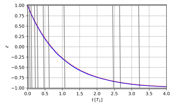
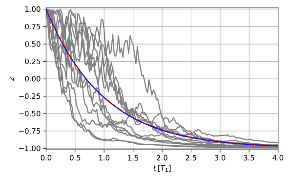
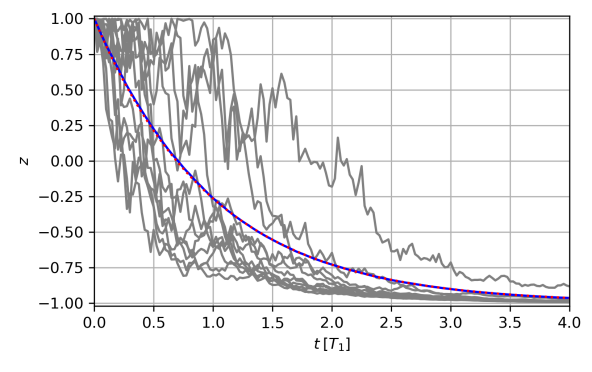
Figure 5: We show simulations of the decay from $\left|e\right\rangle$ to $\left|g\right\rangle$ under ideal measurements, including photodetection (a), heterodyne detection for $\theta=0$ (b), and homodyne detection for $\theta=0$ (c). In every case, we plot a dozen individual trajectories in grey, the average trajectory over an ensemble of 10,000 simulated trajectories in solid blue, and the unmonitored curve integrated from (10) in dotted red. As required by the SME, we see good agreement between the simulated paths averaged over measurement noise realizations (solid blue), and a direct computation of the un–monitored dynamics, which in the present case must simply follow $z(t)=2e^{-\gamma t}-1$ (dotted red). We can see the qualitative similarity between the diffusive homodyne and heterodyne trajectories in (b) and (c), respectively, as well as their stark difference with the jump trajectories generated by photodetection (a); these contrasts are clear and important, as is the average dynamics common to all three schemes, which follows from the shared underlying decay process at the heart of all three measurements considered here. All our simulations are performed by applying our Kraus operator methods.

We also use the Kraus operator to obtain some equations of motion. Consider the exapansion of the Kraus operator itself to $O(dt)$, which reads

$$\hat{M}_{\alpha}e^{|\mathbf{r}|^{2}dt/4}\approx\openone+dt\underbrace{\left(\begin{array}[]{cc}-\tfrac{\gamma}{2}&0\\ \sqrt{\tfrac{\gamma}{2}}(r_{X}+ir_{P})&0\end{array}\right)}_{\hat{m}_{\alpha}}+O(dt^{2})$$ (39)

for $|\mathbf{r}|^{2}=r_{X}^{2}+r_{P}^{2}$. We can strip the Gaussian factor $e^{-|\mathbf{r}|^{2}dt/4}$ from the operator for this purpose, since it appears in both the numerator and denominator of the state update expression (11), and thereby cancels off. Consider the following series of approximations, assuming small $dt$:

$$\begin{split}\rho(t+dt)&\approx\frac{(\openone+\hat{m}_{\alpha}dt)\rho(t)(\openone+\hat{m}_{\alpha}^{\dagger}dt)}{\text{tr}\left((\openone+\hat{m}_{\alpha}dt)\rho(t)(\openone+\hat{m}_{\alpha}^{\dagger}dt)\right)}\\ &\approx\rho+dt\left(\hat{m}_{\alpha}\rho+\rho\hat{m}_{\alpha}^{\dagger}-\rho\>\text{tr}\left(\hat{m}_{\alpha}\rho+\rho\hat{m}_{\alpha}^{\dagger}\right)\right),\end{split}$$ (40)

which can then be rearranged according to $\rho(t+dt)-\rho(t)\approx dt\>\dot{\rho}$, such that

$$\dot{\rho}\approx\hat{m}_{\alpha}\rho+\rho\hat{m}_{\alpha}^{\dagger}-\rho\>\text{tr}\left(\hat{m}_{\alpha}\rho+\rho\hat{m}_{\alpha}^{\dagger}\right).$$ (41)

This can be expressed in Bloch coordinates by

$$\dot{x}=\tfrac{\gamma}{2}x\>z+\sqrt{\tfrac{\gamma}{2}}\left[r_{X}(1+z-x^{2})-r_{P}\>x\>y\right],$$ (42a)

$$\dot{y}=\tfrac{\gamma}{2}y\>z+\sqrt{\tfrac{\gamma}{2}}\left[r_{P}(1+z-y^{2})-r_{X}\>x\>y\right],$$ (42b)

$$\dot{z}=\tfrac{\gamma}{2}(z^{2}-1)-\sqrt{\tfrac{\gamma}{2}}(1+z)\left[r_{X}\>x+r_{P}\>y\right].$$ (42c)

It is then straightforward to make the substitutions $r_{X}=x\sqrt{\gamma/2}+\xi_{X}$ and $r_{P}=y\sqrt{\gamma/2}+\xi_{P}$ (32), and see that these equations from the Kraus operator approach are identical to the Stratonovich equations (28) obtained by conversion from the SME approach; this relationship between a Kraus operator based on Bayesian logic, and the SME, is consistent with previous results for this particular measurement Jordan et al. (2015), and other types of continuous qubit measurements leading to diffusive SQTs Gambetta et al. (2008); Chantasri and Jordan (2015); Korotkov (2016); Lewalle et al. (2017).

Simulations can be generated by applying the state update rule (11) with $\hat{M}_{r}\rightarrow\hat{M}_{\alpha}$, with a pair of readouts drawn from Gaussians of means and variances described above, at each timestep. The resulting stochastic trajectories diffuse as expected, and recreate the required decay dynamics on average, as shown in Fig. 5(b).

IV.3 Generalizations

We consider the addition of a Rabi drive to the qubit (i.e. we now discuss additional tones inducing a unitary rotation in the Bloch sphere) by the addition of a Hamiltonian term $i[\rho,\hat{H}]$ to the SME ($\hbar\rightarrow 1$), or a corresponding operator $\hat{U}=e^{-i\hat{H}dt}$ to the measurement scheme with the Kraus operator (where the resulting equations of motion are insensitive to the order of operations, since they are only to $O(dt)$). Without loss of generality, we use $\hat{H}=\delta\hat{\sigma}_{z}/2+\Omega\hat{\sigma}_{y}/2$, where we have denoted the detuning $\delta=\omega_{\text{qb}}-\omega_{\text{dr}}$, with $\omega_{\text{dr}}$ the frequency of the tone. Such a tone induces a rotation around an axis tilted by an angle $\text{arctan}(\Omega/\delta)$ with respect to the $z$–axis. Note that the assumption in our derivation has been that only photons emitted by the qubit enter the transmission line which leads to the measurement apparatus; the simplest way to imagine engineering a system such that this remains valid with the Rabi drive on, is that the drive is being implemented by a tone which is off–resonant with the qubit/cavity/transmission line, such that the qubit photons couple to the output leading the measurement device only, and the drive photons couple to their own output only. As discussed earlier, this assumption also requires us to have the cavity resonance far from any of the Mollow triplet peaks, which are centered around $\omega_{\text{dr}}$ and $\omega_{\text{dr}}\pm\Omega_{\text{eff}}$, where $\Omega_{\text{eff}}=\sqrt{\Omega^{2}+\delta^{2}}$ is the generalized Rabi frequency; this regime and assumption is necessary if we want to treat the form of the decay channel as being unaffected by the drive. Drives of the type we have discussed apply generically in “resonance fluoresence” scenarios Kimble and Mandel (1976); Naghiloo et al. (2017); Quijandría et al. (2018), as well as any other situation in which additional tones are present in qubit’s cavity (e.g. to implement additional measurements Ficheux et al. (2018)). The situation we have described here is illustrated in Fig. 1(c).

Note that it is possible to generalize this heterodyne measurement by choosing the phase $\theta$ of the LO. The phase $\theta$ is a relative phase between the signal and LO, so it is equivalent to think of a phase plate having been put in the signal line instead of the LO such that $\hat{a}^{\dagger}\rightarrow e^{-i\theta}\hat{a}^{\dagger}$ in (34), with interference against a fixed pump. Mathematically, we can then assign readouts according to

$$\alpha=\sqrt{\frac{dt}{2}}e^{i\theta}(r_{I}-ir_{Q}),$$ (43)

which leads to

$$\begin{split}r_{I}&=\sqrt{\tfrac{\gamma}{2}}(x\cos\theta-y\sin\theta)+\xi_{I},\text{ and}\\ r_{Q}&=\sqrt{\tfrac{\gamma}{2}}(y\cos\theta+x\sin\theta)+\xi_{Q}.\end{split}$$ (44)

The operators for the SME which match the pair of observables we infer from the means of $\mathcal{G}$ are

$$\hat{L}_{I}=\sqrt{\tfrac{\gamma}{2}}e^{-i\theta}\hat{\sigma}_{-},\text{ and }\hat{L}_{Q}=i\sqrt{\tfrac{\gamma}{2}}e^{-i\theta}\hat{\sigma}_{-}.$$ (45)

We see that changing the phase $\theta$ between the signal and LO effectively rotates the quadrature pair we measure. We have here used notation such that $r_{I}=r_{X}$ and $r_{Q}=r_{P}$ for the choice $\theta=0$. The relationship between the Kraus operator equations of motion and SME equations of motion (Itô or Stratonovich) which we found in the $\theta=0$ case above, hold for arbitrary $\theta$.

We have reviewed the most basic features of an idealized heterodyne measurement. For a more advanced treatment of this system, refer to Jordan et al. (2015); we will now turn our attention to applying the framework we have just developed to homodyne measurement.

V Single–Qubit Homodyne Fluorescence Trajectories

Several experiments Naghiloo et al. (2017, 2016); Tan et al. (2017); Naghiloo et al. (2020) and some theory Bolund and Mølmer (2014) have been published about homodyne fluorescence measurement; we will develop our theory examples here far enough to compare them directly with the simplest experimental results.

V.1 Kraus Operator and Measurement Dynamics

Homodyne detection again involves interfering our signal with a strong LO. Practically, instead of amplifying both quadratures of the resulting signal as in heterodyne detection, homodyne detection involves amplifying one quadrature and de-amplifying the other Tyc and Sanders (2004) (“phase-sensitive” amplification). This procedure amounts to squeezing out the quadrature that isn’t measured, such that in the limit of ideal squeezing we project our signal onto a single quadrature’s eigenstate, instead of onto a coherent state Wiseman (1996); Wiseman and Milburn (2010). This yields a single readout signal, rather than the pair which arise in the heterodyne case. We will follow the same recipe as in the heterodyne case, except that we project onto a final state $\left|X\right\rangle$ (the eigenstate of the $\hat{X}=(\hat{a}^{\dagger}+\hat{a})/\sqrt{2}$ operator in the quadrature space), instead of the coherent state $\left|\alpha\right\rangle$. Again, those unfamiliar with this phase space terminology may wish to consult e.g. Ref. Silberhorn (2007). For dimensionless $X$, recall that we have the following solutions to the quantum harmonic oscillator, which models the field mode:

$$\langle X|0\rangle=\pi^{-\frac{1}{4}}e^{-X^{2}/2},\text{ and }\langle X|1\rangle=\pi^{-\frac{1}{4}}\sqrt{2}Xe^{-X^{2}/2}.$$ (46)

Projecting onto the general fluorescence operator, and suppressing the factors $\pi^{-\tfrac{1}{4}}$ on all terms, we get

$$\hat{M}_{x}=\left\langle X\right|\left(\begin{array}[]{cc}\sqrt{1-\epsilon}&0\\ \sqrt{\epsilon}\hat{a}^{\dagger}&1\end{array}\right)\left|0\right\rangle=e^{-X^{2}/2}\left(\begin{array}[]{cc}\sqrt{1-\epsilon}&0\\ \sqrt{2\epsilon}X&1\end{array}\right).$$ (47)

Then using a readout substituted in according to

$$X\rightarrow\sqrt{\frac{dt}{2}}r,$$ (48)

we find that the POVM is normalized, i.e.

$$\sqrt{\frac{dt}{2\pi}}\int_{-\infty}^{\infty}dr\>\hat{M}_{x}^{\dagger}\hat{M}_{x}=\openone.$$ (49)

The relationship between $X$ and $r$ is again set based on comparing the readout statistics with LO’s shot noise, as discussed in appendix A. Those readout statistics can be readily understood from the expression

$$\mathcal{G}_{hom}=-\tfrac{1}{2}\left(r-\sqrt{\gamma}x\right)^{2}-\tfrac{\gamma}{2}(1+z-x^{2}),$$ (50)

which again comes from expanding the logarithm of $\text{tr}(\hat{M}_{x}\rho\hat{M}_{x}^{\dagger})$. We infer that projecting onto $\left|X\right\rangle$ in the photon space leads to a signal related to $x$ in the qubit space, since $r$ has a mean $\sqrt{\gamma}x$, and variance $1/dt$.

As before, we may take $\hat{a}^{\dagger}\rightarrow\hat{a}^{\dagger}e^{-i\theta}$ to generalize the choice of measured quadrature, yielding an operator

$$\hat{M}_{x}=\left(\frac{dt}{2\pi}\right)^{\frac{1}{4}}e^{-r^{2}dt/4}\left(\begin{array}[]{cc}\sqrt{1-\gamma dt}&0\\ dt\sqrt{\gamma}\>re^{-i\theta}&1\end{array}\right),$$ (51)

which still generates a proper POVM. Expanding the log–probability density for the readout gives us

$$\begin{split}\mathcal{G}_{hom}^{\theta}=&-\tfrac{1}{2}\left[r-\sqrt{\gamma}(x\cos\theta-y\sin\theta)\right]^{2}\\ &-\tfrac{\gamma}{2}(1+z-(x\cos\theta-y\sin\theta)^{2});\end{split}$$ (52)

thus the mean of the Gaussian in $r$ matches the signal given by $\hat{L}+\hat{L}^{\dagger}=\sqrt{\gamma}(\hat{\sigma}_{x}\cos\theta-\hat{\sigma}_{y}\sin\theta)$ for the SME operator $\hat{L}=\sqrt{\gamma}e^{-i\theta}\hat{\sigma}_{-}$.

We proceed to find the equations of motion. Note that we can approximate $\hat{M}_{x}$ as we did $\hat{M}_{\alpha}$ (39), such that

$$\left(\begin{array}[]{cc}\sqrt{1-\gamma dt}&0\\ dt\sqrt{\gamma}\>re^{-i\theta}&1\end{array}\right)\approx\openone+dt\underbrace{\left(\begin{array}[]{cc}-\tfrac{\gamma}{2}&0\\ \sqrt{\gamma}\>re^{-i\theta}&0\end{array}\right)}_{\hat{m}_{x}}+O(dt^{2}).$$ (53)

Then by the logic of (40) and (41) we may derive equations of motion in terms of Bloch coordinates

$$\dot{x}=\tfrac{\gamma}{2}xz+\Omega z-\delta y+r\sqrt{\gamma}\left[(1+z-x^{2})\cos\theta+xy\sin\theta\right],$$ (54a)

$$\dot{y}=\tfrac{\gamma}{2}yz+\delta x+r\sqrt{\gamma}\left[(y^{2}-z-1)\sin\theta-xy\cos\theta\right],$$ (54b)

$$\dot{z}=\tfrac{\gamma}{2}(z^{2}-1)-\Omega x+r\sqrt{\gamma}(z+1)\left[y\sin\theta-x\cos\theta\right].$$ (54c)

We have again used a Rabi drive characterized by $\hat{H}=\Omega\hat{\sigma}_{y}/2+\delta\hat{\sigma}_{z}/2$, or $\hat{U}\approx\openone-i\Omega\hat{\sigma}_{y}dt/2-i\delta\hat{\sigma}_{z}dt/2$. As above, these equations are consistent with those derived from the SME (23), using $\hat{L}=\sqrt{\gamma}e^{-i\theta}\hat{\sigma}_{-}$, provided the SME output is correctly interpreted as an Itô equation, whose Stratonovich form then matches the above exactly. Simulated trajectories for the case $\theta=0$ and $\Omega=0$ are shown in Fig. 5(c), and demonstrate good agreement with expectations, as in the previous cases.

V.2 Inefficient Measurements

Inefficient measurement is easily included in the SME (23), and is completely described by the dimensionless parameter $\eta\in[0,1]$. In the Kraus operator picture, we must modify the amplitude of the signal going into the measurement apparatus; we will find a case intermediate between perfect measurements (11) and no measurement (20), reflecting that some fraction of the information is lost rather than collected. A straightforward way to represent this is with an unbalanced beamsplitter placed in front of our (still otherwise ideal) measurement device, as shown in Fig. 1(d). If $\hat{a}^{\dagger}$ creates a photon in the emitted field mode, the beamsplitter transforms it according to

$$\hat{a}^{\dagger}\rightarrow\sqrt{\eta}\>\hat{a}_{s}^{\dagger}+\sqrt{1-\eta}\>\hat{a}_{\ell}^{\dagger},$$ (55)

where the surviving signal $\hat{a}_{s}^{\dagger}$ goes to the detector with probability $\eta$, but the information in channel $\hat{a}_{\ell}^{\dagger}$ is lost with probability $1-\eta$, and outcomes (all of which could have occurred) in the latter channel must be traced out. We will do the trace of the lost channel in the Fock basis for simplicity (a sum of two terms is simpler than an integral over a continuous homodyne or heterodyne readout, although averaging over any complete set of hypothetical measurement outcomes is technically correct). The scheme we are describing, for homodyne detection with efficiency $\eta$, can be implemented with a pair of operators

$$\hat{M}_{xj}=\left\langle X_{s}j_{\ell}\right|\left(\begin{array}[]{cc}\sqrt{1-\epsilon}&0\\ \sqrt{\epsilon\eta}\>\hat{a}_{s}^{\dagger}+\sqrt{\epsilon(1-\eta)}\>\hat{a}_{\ell}^{\dagger}&1\end{array}\right)\left|00\right\rangle,$$ (56)

for Fock states $j=0,1$ in the lost mode, i.e.

$$\hat{M}_{x0}=e^{-X^{2}/2}\left(\begin{array}[]{cc}\sqrt{1-\epsilon}&0\\ \sqrt{2\epsilon\eta}X&1\end{array}\right),$$ (57a)

$$\hat{M}_{x1}=e^{-X^{2}/2}\left(\begin{array}[]{cc}0&0\\ \sqrt{\epsilon(1-\eta)}&0\end{array}\right),$$ (57b)

with a state update rule

$$\rho(t+dt)=\frac{\hat{M}_{x0}\rho(t)\hat{M}_{x0}^{\dagger}+\hat{M}_{x1}\rho(t)\hat{M}_{x1}^{\dagger}}{\text{tr}\left(\hat{M}_{x0}\rho(t)\hat{M}_{x0}^{\dagger}+\hat{M}_{x1}\rho(t)\hat{M}_{x1}^{\dagger}\right)}.$$ (58)

The measured homodyne signal is computed according to projection onto the states $\left|X\right\rangle$ exactly as above, and a drive could be added with unitaries in the same manner as above. The new operators (56) again denote a well–defined measurement, in that they form POVM elements, i.e.

$$\int_{-\infty}^{\infty}dX\sum_{j=0,1}\hat{M}_{xj}^{\dagger}\hat{M}_{xj}\propto\openone.$$ (59)

We find the same agreement between the expansion of the state update (58) to $O(dt)$, and the SME with finite $\eta$ (converted to its Stratonovich form), as in every case discussed. Thus the description of $\eta$ supposed by Fig. 1(d) and (55) is entirely equivalent to the description implicit in the SME, and clarifies the meaning of measurement “inefficiency”.

This picture of inefficiency is also readily connected to scenarios in which several observers simultaneously make measurements, and each gets only partial information Jacobs and Steck (2006); Dziarmaga et al. (2004); Harrington et al. (2019). One can imagine that an observer lives at each output of the beamsplitter in Fig. 1(d), each recieving some proportion of the information about the qubit carried by the decay process as they make measurements. If they do not share their results, each will have a different estimate of the qubit’s evolution conditioned on their partial information, and tracing out over the other observer’s measurement record which they do not have access to. Either of their estimates could be compared to some hypothetical “true” evolution which an observer able to access all the relevant measurement records could compute. In practice, it is effectively impossible to have a perfectly efficient measurement in any experiment, and some information is always irretrievably lost to the environment through any channel from which the primary system is not perfectly isolated (generically, this is “decoherence”). The methods we have presented here can readily be adapted to the kind of multiple–observer situation we have just described; this includes situations which involve both jumps and diffusion, due to different observers making different types of measurements (see e.g. appendix B of Lewalle et al. (2019a), or Kuramochi et al. (2013)). Such scenarios have recently been fruitfully investigated in the context of quantum state smoothing Guevara and Wiseman (2015); Chantasri et al. (2019); Guevara and Wiseman .

We perform simulations which include measurement inefficiency, which are shown in Fig. 7, and discussed further in connection with the “optimal path” techniques we develop shortly. Measurement inefficiency leads to decay that is qualitatively the same as in the ideal case discussed in Fig. 5, except that instead of trajectories being restricted to pure states on the surface of the Bloch sphere, as in the $\eta=1$ case, they instead move stochastically on the surface of an ellipsoid which contracts towards $\left|g\right\rangle$ over time as information is lost in the $\eta<1$ case. Qualitative agreement between these simulated results shown in Fig. 7 and those obtained in experiment for either the homodyne Naghiloo et al. (2016) or heterodyne Campagne-Ibarcq et al. (2016a) detection can be verified at a glance, and a quantitative understanding of this will be developed shortly.

As we have now successfully adapted and extended our presentation of basic methods for pertaining to quantum trajectories to the homodyne detection case, and established that they behave correctly, we can proceed by extending our analysis of this system into new examples which can introduce and highlight particular topics in the recent literature.

VI Special Topics and Further Examples

We will focus on connections to two areas, using homodyne fluorescence detection as our example of choice; first we describe how this example relates to recent work about the arrow of time in quantum measurement, which connects to work on fluctuation theorems for quantum trajectories, and the growing area of quantum thermodynamics more generally; second we will describe how “most–likely paths” can be derived from diffusive quantum trajectory dynamics using a variational principle.

VI.1 Time reversal symmetry and the arrow of time

How does an arrow of time emerge from microscopically time–reversible physical laws? The issue has been raised in the context of continuous quantum measurements Dressel et al. (2017); Manikandan and Jordan (2019); Manikandan et al. (2019); Harrington et al. (2019), and applies more broadly across many disciplines within physics Hawking (1985); Maccone (2009); Lebowitz (1993). In the quantum measurement case, one could pose this question as a game; a quantum trajectory is shown like a movie, forward and backward, and the goal of the game is to infer the direction in which the movie was originally recorded. We will find that the equations of motion are time–symmetric, (e.g. as in Hamiltonian dynamics), such that both the forward and backward movies both depict legitimate dynamics; this is not the whole story however, as the backward evolution (i.e. “wavefunction uncollapse”) does not necessarily occur with the same probability Jordan and Korotkov (2010); Korotkov and Jordan (2006). This leads to a natural discriminator for the arrow of time in terms of the probabilities of occurrence of forward and backward trajectories of the monitored quantum system, as developed in Refs. Dressel et al. (2017); Manikandan and Jordan (2019). Assuming no prior bias, we could use the measurement record as an additional tool to improve our inference about the direction in which the quantum state dynamics is originally recorded Dressel et al. (2017) (by analogy, the sound track for a movie could help us understand in which direction it is meant to run). Such an approach is fundamentally connected to the time–symmetry of underlying dynamical equations describing the measurement, and connects to the arrow of time analysis pertinent to the thermodynamics of small systems Chernyak et al. (2006); Manikandan et al. (2019).

Fluorescence appears to exhibit a clear arrow of time, and therefore the time–reversibility of continuously monitored fluorescence dynamics may seem rather surprising. For this reason, here we detail the time symmetry analysis of dynamical equations (54) which describe homodyne measurement of fluorescence, using the approach presented in Ref. Manikandan and Jordan (2019), wherein similar and detailed analysis was performed for the heterodyne case. The time–reversed dynamics can be considered as a legitimate measurement dynamics, starting from the time–reversed final state $\Theta|\psi_{f}\rangle$, evolving through the time–reversed counterpart of the forward sequence of states, back to the time–reversed initial state $\Theta|\psi_{i}\rangle$. The measurement operators of the backward dynamics are related to the forward dynamics by a Hermitian conjugate operation, i.e. $\hat{M}_{B}=\hat{M}_{F}^{\dagger}$; therefore the dynamical equations which describe the backward dynamics are also similar to the retrodicted dynamical equations Tan et al. (2015), but starting from the time–reversed final state. We may write the retrodicted dynamical equations corresponding to a homodyne measurement, where the quantum state is updated by

$$\underaccent{\bar}{\rho}(\underaccent{\bar}{t}+\underaccent{\bar}{dt})=\frac{\hat{M}_{x}^{\dagger}\underaccent{\bar}{\rho}(\underaccent{\bar}{t})\hat{M}_{x}}{\text{tr}[\hat{M}_{x}^{\dagger}\underaccent{\bar}{\rho}(\underaccent{\bar}{t})\hat{M}_{x}]}.$$ (60)

We have parameterized the single–qubit density matrix $\underaccent{\bar}{\rho}$ with Bloch coordinates according to

$$\underaccent{\bar}{\rho}=\frac{1}{2}\left(\begin{array}[]{cc}1+\underaccent{\bar}{z}&\underaccent{\bar}{x}-i\underaccent{\bar}{y}\\ \underaccent{\bar}{x}+i\underaccent{\bar}{y}&1-\underaccent{\bar}{z}\end{array}\right).$$ (61)

Using the form of measurement operators given in Eq. (51) The dynamical equations now take the form,

$$\dot{\underaccent{\bar}{x}}=\tfrac{\gamma}{2}\underaccent{\bar}{x}\underaccent{\bar}{z}+r\sqrt{\gamma}\left[(1-\underaccent{\bar}{z}-\underaccent{\bar}{x}^{2})\cos\theta+\underaccent{\bar}{x}\underaccent{\bar}{y}\sin\theta\right],$$ (62a)

$$\dot{\underaccent{\bar}{y}}=\tfrac{\gamma}{2}\underaccent{\bar}{y}\underaccent{\bar}{z}+r\sqrt{\gamma}\left[(\underaccent{\bar}{y}^{2}+\underaccent{\bar}{z}-1)\sin\theta-\underaccent{\bar}{x}\underaccent{\bar}{y}\cos\theta\right],$$ (62b)

$$\dot{\underaccent{\bar}{z}}=\tfrac{\gamma}{2}(\underaccent{\bar}{z}^{2}-1)+r\sqrt{\gamma}(-\underaccent{\bar}{z}+1)\left[-\underaccent{\bar}{y}\sin\theta+\underaccent{\bar}{x}\cos\theta\right].$$ (62c)

Note that the retrodicted equations under the time-reversal operation, $\underaccent{\bar}{x}\rightarrow-x,~{}\underaccent{\bar}{y}\rightarrow-y,~{}\underaccent{\bar}{z}\rightarrow-z$, and $\underaccent{\bar}{t}\rightarrow T-t$ (i.e., $\underaccent{\bar}{dt}\rightarrow-dt$) looks exactly like the forward dynamical equations (54), demonstrating their time–reversal invariance; we have eliminated the drive characterized by $\Omega$ and $\delta$ in the equations above for brevity, but including it does not affect the result. Time reversal symmetry of the dynamical equations suggests that the forward dynamics and the reverse dynamics both represent a physical quantum trajectory on the Bloch sphere. Given the measurement record, one can associate a probability each to the forward and backward trajectories, which can be used to infer an arrow of time for the measurement dynamics, and subsequently characterize the irreversibility of homodyne measurement of fluorescence using the associated fluctuation theorems Dressel et al. (2017); Manikandan and Jordan (2019); Manikandan et al. (2019).

We can expand on this story somewhat by noting that our diffusive trajectories in Fig. 5(b,c) do not diffuse monotonically downward from $\left|e\right\rangle$ towards $\left|g\right\rangle$. This suggests that the measurement process can actually cause the probability of the qubit being found in the more energetic of its states to rise in some realizations. While the average decays monotonically, fluctuations make this question of an arrow of time non–trivial in individual realizations; the probability of sustained re-excitation over a long period is low, but estimates of the arrow of time using only a short window of the evolution cannot necessarily be made with high confidence; rare events can decieve, and something resembling a “wavefunction uncollapse” is not merely hypothetical in this system. Such behavior has been noted in the literature Bolund and Mølmer (2014); while it may be initially intuitively challenging, this effect is perfectly correct, and reflects the nature of the information we get about the field when we make a weak ($dt\ll T_{1}$) quadrature measurement, and its backaction. A truly detailed description of the thermodynamics of quantum measurements or trajectories falls beyond our present scope, but is a fascinating area related to the questions we have discussed here, and enjoying increased recent research interest Cottet et al. (2017); Elouard et al. (2017a, b); Naghiloo et al. (2020); Elouard and Jordan (2018); Masuyama et al. (2018); Monsel et al. (2018, 2019); Mohammady et al. (2019). We encourage the curious reader to explore further.

VI.2 A Variational Principle for Quantum Trajectories

Optimal paths (OPs) Chantasri et al. (2013); Chantasri and Jordan (2015); Jordan et al. (2015); Areeya Chantasri (2016); Lewalle et al. (2017, 2018) have recently been used to elucidate a variety of quantum trajectory phenomena. We will here give a brief overview of their derivation, using the CDJ (Chantasri/Dressel/Jordan) path integral Chantasri et al. (2013), and then apply the formalism to the homodyne fluorescence examples we have developed above.

VI.2.1 Derivation of Optimal Paths

OPs can be understood as the path extremizing the probability to get from one given quantum state $\mathbf{q}_{i}$ to another $\mathbf{q}_{f}$ in a particular time interval, under the dynamics due to backaction from the continuous weak quantum measurement. The vector $\mathbf{q}$ parameterizes the quantum state, and here denotes coordinates on the Bloch sphere. Typically OPs will be most–likely paths (MLPs), which maximize the probability of the measurement record connecting the given boundary conditions according to an action–extremization principle. OPs should be confused neither with a globally most–likely path (i.e. the particular MLP post–selected on the most likely final state after a given time interval), or with an average path. Details about numerical procedures to extract an MLP from data, which corresponds to the theory we are about to develop, can be found in appendix B.

To begin, we explain how the path probability can be written in terms of an effective action, which can then be extremized according to a variational principle. We may write an expression for the probability of a quantum trajectory, which moves from $\mathbf{q}_{i}$ to $\mathbf{q}_{f}$ through a discrete sequence of measurements as

$$\begin{split}\mathcal{P}(\{\mathbf{q}\},\{\mathbf{r}\}|\mathbf{q}_{i},\mathbf{q}_{f})=\delta(\mathbf{q}_{i}-\mathbf{q}_{0})\delta(\mathbf{q}_{f}-\mathbf{q}_{n})\left\{\prod_{k=0}^{n-1}\wp(\mathbf{r}_{k}|\mathbf{q}_{k})\wp(\mathbf{q}_{k+1}|\mathbf{q}_{k},\mathbf{r}_{k})\right\}.\end{split}$$ (63)

The $\delta$–functions at the initial and final points impose the boundary conditions. The indices $k$ run over time, such that if $\rho_{k}=\rho(t)$, then $\rho(t+dt)=\rho_{k+1}$ and so on. The stochastic element of the dynamics arises in drawing the readout from the probability density determined by the denominator of the state update expression (11), i.e. $\wp(\mathbf{r}_{k}|\rho_{k})\propto\text{tr}(\hat{M}_{\mathbf{r}_{k}}\rho_{k}\hat{M}_{\mathbf{r}_{k}}^{\dagger})$, where $\hat{M}_{\mathbf{r}_{k}}$ could generically be any Kraus operator describing a weak measurement. We describe the deterministic update of the quantum state given the stochastic readout $\mathbf{r}_{k}$ according to $\wp(\mathbf{q}_{k+1}|\mathbf{q}_{k},\mathbf{r}_{k})=\delta(\mathbf{q}_{k+1}-\mathbf{q}_{k}-dt\>\mathcal{F}[\mathbf{q}_{k},\mathbf{r}_{k}])$, where $\dot{\mathbf{q}}=\mathcal{F}[\mathbf{q},\mathbf{r}]$ is an equation of motion, e.g. like (54). Recall that a $\delta$–function may be written $\delta(\mathbf{q})=(2\pi i)^{-\text{dim}(\mathbf{q})}\int_{-i\infty}^{i\infty}d\mathbf{p}\>\exp\left[-\mathbf{p}\cdot\mathbf{q}\right]$, where $\text{dim}(\mathbf{q})$ is the dimension of $\mathbf{q}$, and $d\mathbf{p}=dp_{1}\;dp_{2}\;...\;dp_{\text{dim}(\mathbf{q})}$. We apply this identity to all $\delta$–functions in (63), such that in the time–continuum limit we have a Feynman–like path integral, in which we effectively sum over all possible quantum trajectories which obey the given boundary conditions, i.e.

$$\begin{split}\mathcal{P}&=\underset{n\rightarrow\infty}{\text{lim}}\;\underset{dt\rightarrow 0}{\text{lim}}\;\mathcal{N}\idotsint\limits_{-i\infty}^{i\infty}\left(\prod_{k=0}^{n-1}d\mathbf{p}_{k}\right)\exp\bigg{[}\mathcal{B}+\sum_{k=0}^{n-1}\left(-\mathbf{p}_{k}\cdot(\mathbf{q}_{k+1}-\mathbf{q}_{k}-dt\>\mathcal{F}_{k})+\ln\wp(\mathbf{r}_{k}|\mathbf{q}_{k})\right)\bigg{]}\\ &\propto\int\mathcal{D}[\mathbf{p}]\exp\left[\mathcal{B}+\int_{0}^{T}dt\left(-\mathbf{p}\cdot\dot{\mathbf{q}}+\mathbf{p}\cdot\mathcal{F}[\mathbf{q},\mathbf{r}]+\mathcal{G}[\mathbf{q},\mathbf{r}]\right)\right]\\ &=\int\mathcal{D}[\mathbf{p}]\exp\left[\mathcal{B}+\int_{0}^{T}dt(\mathcal{H}(\mathbf{q},\mathbf{p},\mathbf{r})-\mathbf{p}\cdot\dot{\mathbf{q}})\right]=\int\mathcal{D}[\mathbf{p}]\exp\left(\mathcal{B}+\mathcal{S}[\mathbf{q},\mathbf{p},\mathbf{r}]\right)\end{split}$$ (64)

for $\mathcal{N}=(2\pi i)^{-(n+2)\cdot\text{dim}(\mathbf{q})}$, and where $\mathcal{D}[\mathbf{p}]$ arises from the infinite product of the $d\mathbf{p}_{k}(2\pi i)^{-\text{dim}(\mathbf{q}_{k})}$. We use the shorthand $\mathcal{B}=-\mathbf{p}_{-1}\cdot(\mathbf{q}_{0}-\mathbf{q}_{i})-\mathbf{p}_{n}\cdot(\mathbf{q}_{n}-\mathbf{q}_{f})$ for the boundary terms, and the shorthand $\mathcal{G}$ for the expansion to $O(dt)$ of the log–probability for the readouts $\ln\wp(\mathbf{r}|\mathbf{q})$ (see e.g. (52)). This relates a trajectory probability $\mathcal{P}$ to a “stochastic action” $\mathcal{S}$. That action is expressed in terms of a Hamiltonian $\mathcal{H}=\mathbf{p}\cdot\mathcal{F}+\mathcal{G}$.

We can then see that extremizing the probability corresponds to extremizing $\mathcal{S}$. Action extremization in this case can be expressed much the same way as it is in classical mechanics, such that

$$\begin{split}\delta\mathcal{S}&=0\\ &=\delta\int_{0}^{T}dt\left(-\mathbf{p}\cdot\dot{\mathbf{q}}+\mathcal{H}(\mathbf{q},\mathbf{p},r)\right)=\int_{0}^{T}dt\left(\frac{\partial\mathcal{H}}{\partial\mathbf{q}}\cdot\delta\mathbf{q}+\frac{\partial\mathcal{H}}{\partial\mathbf{p}}\cdot\delta\mathbf{p}+\frac{\partial\mathcal{H}}{\partial\mathbf{r}}\cdot\delta\mathbf{r}-\mathbf{p}\cdot\delta\dot{\mathbf{q}}-\dot{\mathbf{q}}\cdot\delta\mathbf{p}\right)\\ &=\mathbf{p}\cdot\delta\mathbf{q}|_{0}^{T}+\int_{0}^{T}dt\bigg{[}\delta\mathbf{q}\cdot\left(\frac{\partial\mathcal{H}}{\partial\mathbf{q}}+\dot{\mathbf{p}}\right)+\delta\mathbf{p}\cdot\left(\frac{\partial\mathcal{H}}{\partial\mathbf{p}}-\dot{\mathbf{q}}\right)+\delta\mathbf{r}\cdot\frac{\partial\mathcal{H}}{\partial\mathbf{r}}\bigg{]},\end{split}$$ (65)

which indicates that the OPs obey the equations

$$\dot{\mathbf{q}}=\frac{\partial\mathcal{H}}{\partial\mathbf{p}},\quad\dot{\mathbf{p}}=-\frac{\partial\mathcal{H}}{\partial\mathbf{q}},\quad\frac{\partial\mathcal{H}}{\partial\mathbf{r}}\bigg{|}_{\mathbf{r}^{\star}}=0.$$ (66)

These are Hamilton’s usual equations in the Bloch coordinates $\mathbf{q}$ and conjugate variables $\mathbf{p}$, plus an additional equation which stipulates that the stochastic readouts be optimized, leading to some smooth $\mathbf{r}^{\star}$ instead of the stochastic $\mathbf{r}$. The OPs are thus smooth curves, and are solutions to a Hamiltonian dynamical system of ordinary, rather than stochastic, differential equations. The OPs are themselves possible quantum trajectories (since $\dot{\mathbf{q}}=\mathcal{F}$ is preserved, by construction), even though the optimal readouts $\mathbf{r}^{\star}$ are smooth functions of time, rather than the stochastic readouts which occur in individual runs of an experiment. The Hamiltonian structure of the OP dynamics implies that, absent any explicitly time–dependent parameters, there is a conserved “stochastic energy” $E=\mathcal{H}$ associated with an OP.

The “momenta” $\mathbf{p}$ conjugate to the generalized Bloch coordinates $\mathbf{q}$, which arise in this optimization process, warrant further attention. The $\mathbf{p}$ are not directly measurable, but play a substantive mathematical role, in that they effectively generate displacements in the quantum state $\mathbf{q}$ according to the optimal measurement record $\mathbf{r}^{\star}$. They appear as the variables conjugate to $\mathbf{q}$ in the Fourier representation of the $\delta$–functions, and could be understood and Lagrange multipliers in the optimization process. They are perhaps best understood in analogy with classical optics, however: just as we have expressed a diffusive process in terms of an action, the underlying wave process in classical optics can be expressed as an action; extremization in the latter scenario leads to a ray description. Our OPs are related to the underlying diffusive process described above in much the same way that a ray description of light is related to the underlying wave optics process. Diffusive SQTs arrive at final states with a variety of probabilities (and the action representing this is real), whereas optical paths leading to different positions arrive with different phases, exhibiting interference (and the subsequent action in this case is imaginary). Continuing with this analogy, we could imagine that rays leave a source in different directions, i.e. with different wave–vectors (OPs leave their initial state $\mathbf{q}_{i}$ with a range of initial momenta $\mathbf{p}_{i}$); we may pick out a particular ray or subset of rays by choosing a particular initial wave–vector, or by choosing a final position to which they connect (a particular OP can be selected by choosing a value of $\mathbf{p}_{i}$, or by choosing a $\mathbf{q}_{f}$ at a later time). Thus, the degree of freedom in choosing an initial momentum $\mathbf{p}_{i}$ is the same degree of freedom which allows for post–selections to many $\mathbf{q}_{f}$; the mapping between the two is not necessarily one–to–one (see our work on “multipaths” for clarification of this point Lewalle et al. (2017); Naghiloo et al. (2017); Lewalle et al. (2018)). In a phase space with $N$ coordinates $\mathbf{q}$ and $N$ momenta $\mathbf{p}$ (a $2N$–dimensional phase space), the set of paths evolving from all $\mathbf{p}_{i}$ with a fixed $\mathbf{q}_{i}$ defines an $N$–dimensional Lagrangian manifold (LM) within the phase space; such a manifold can be understood as containing all of the possible dynamics originating from the state $\mathbf{q}_{i}$ in the OP description, i.e. such an LM explores the full space of optimal readouts $\mathbf{r}^{\star}$, just as the underlying diffusive process may explore the full space of stochastic measurement records. Our focus now will be on applying this formalism to our homodyne fluorescence measurement; some work in this vein, albeit with a different emphasis, appears in Ref. Naghiloo et al. (2017).

VI.2.2 Optimal Paths for Homodyne Fluorescence Trajectories

Notice that the system of equations (54) can be simplified straightforwardly; $\dot{y}=0$ if $y=0$ and $\theta=0$, and then all the dynamics are in the $xz$–plane of the Bloch sphere. It is then easy to write down a stochastic Hamiltonian

$$\begin{split}\mathcal{H}_{hom}^{xz}=&\quad p_{x}\left(\tfrac{\gamma}{2}xz+r\sqrt{\gamma}\left[1+z-x^{2}\right]\right)\\ &+p_{z}\left(\tfrac{\gamma}{2}(z^{2}-1)-r\sqrt{\gamma}(z+1)x\right)\\ &-\tfrac{1}{2}\left(r-\sqrt{\gamma}x\right)^{2}-\tfrac{\gamma}{2}(1+z-x^{2}),\end{split}$$ (67)

for the OP dynamics using formulas we have already derived above (with $\Omega=0=\delta$, and $\eta=1$) to describe the ideal measurement, its backaction, and statistics. The optimal readout obeys $\partial_{r}\mathcal{H}_{hom}^{xz}|_{r^{\star}}=0$, which we solve to obtain

$$r^{\star}=\sqrt{\gamma}\left(x+p_{x}(1+z-x^{2})-xp_{z}(1+z)\right);$$ (68)

we see that we have the signal $\sqrt{\gamma}x$, plus some additional terms which depend on the conjugate momenta $p_{x}$ and $p_{z}$, which implement the optimized effect of the noise (as discussed above).

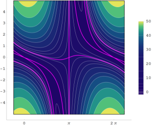
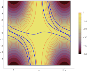
Figure 6: We show the OP phase space in $\vartheta$ and $p$, for an ideal homodyne measurement of the qubit fluorescence, and with $\gamma=1~{}\mathrm{MHz}$ and $\Omega=0$. We plot the stochastic Hamiltonian in the top panel. Contours are lines of constant “stochastic energy” $E=\mathcal{H}^{\vartheta\star}_{hom}$ in $\mathrm{MHz}$, which are solutions to the OP dynamics. Fixed points appear at $\vartheta=0$ and $\pi$, at $p=0$; the separatrices which pass through these points are shown in magenta. Those separatrices bound off distinct regions X, Y, and Z; each has some distinct behavior, all of them ultimately lead their paths to the ground state $\theta=\pi$. The regions come in pairs due to the symmetry of the phase space, where + denotes that the paths in that region approach the ground state from below (with $\vartheta$ increasing), and their mirror images - approach from above (with $\vartheta$ decreasing). We plot $\dot{\mathcal{S}}=\mathcal{H}^{\vartheta\star}_{hom}-p\dot{\vartheta}$ in the bottom panel; this quantity can be regarded as an approximate rate of probability decay, such that paths which spend time in regions of more negative $\dot{\mathcal{S}}$ correspond to sequences of measurement results which are relatively less likely. The OP phase space regions are overlaid on the bottom plot in blue for reference. Comparing the two panels, we see that we can associate paths with larger stochastic $E$ with less–likely dynamics (as a rule of thumb).

We can simplify the equations even more. Consider a change to polar coordinates according to the canonical transformation

$$\begin{array}[]{lcc}x&\rightarrow&R\sin\vartheta\\ z&\rightarrow&R\cos\vartheta\\ p_{x}&\rightarrow&p_{R}\sin\vartheta+p\cos\vartheta/R\\ p_{z}&\rightarrow&p_{R}\cos\vartheta-p\sin\vartheta/R\end{array}$$ (69)

which preserves the Poisson brackets between all of the pairs of conjugate variables. Then we see that for the choice $R=1$ and $p_{R}=0$, we have $\dot{R}=\partial_{p_{R}}\mathcal{H}_{hom}^{\star,R\vartheta}=0$, meaning that we can look at dynamics purely on the great circle of the Bloch sphere at $R=1$ (pure states), where states are parameterized entirely by a single coordinate $\vartheta$ (with $\vartheta=0\leftrightarrow\left|e\right\rangle$ and $\vartheta=\pi\leftrightarrow\left|g\right\rangle$). Making this transformation, and subtituting in the optimal readout such that $\mathcal{H}^{\star}=\mathcal{H}|_{r=r^{\star}}$, we obtain the Hamiltonian

$$\begin{split}\mathcal{H}_{hom}^{\vartheta\star}=&p^{2}\left(\gamma\cos\vartheta+\frac{1}{4}\gamma\cos(2\vartheta)+\frac{3\gamma}{4}\right)\\ &+p\left(\frac{3}{2}\gamma\sin\vartheta+\frac{1}{2}\gamma\sin(2\vartheta)\right)\\ &-\frac{1}{2}\gamma\cos\vartheta-\frac{1}{4}\gamma\cos(2\vartheta)-\frac{\gamma}{4},\end{split}$$ (70)

which generates the OPs in the simplest case we can consider for this system.

The phase space for this Hamiltonian is plotted in Fig. 6, along with the time–derivative of the stochastic action $\mathcal{S}$ which is extremized by the OP dynamics (effectively, $\dot{\mathcal{S}}$ gives an approximate representation of the probability cost involved with traversing certain regions of the OP phase space). A careful reading of these plots can provide an insightful overview of the system dynamics. First, we can immediately infer a rule of thumb: OPs with higher stochastic energy generically correspond to events which occur with lower probabilities (this is true to the extent that regions of large $E$ correspond to regions of more–negative $\dot{\mathcal{S}}$). Secondly, we see that all paths in the OP phase space eventually approach $\left|g\right\rangle$ ($\vartheta=\pi$) in the long–time limit, as we expect they must; there are possibilities for this to occur in either direction around the Bloch sphere with some probabilities, but these pure–state OPs never cross through $\vartheta=\pi$. The uni–directionality of the flow towards $\left|g\right\rangle$ after $t\gg T_{1}$ reflects our intuition that there should be a statistical arrow of time in the measurement–induced dynamics, as is discussed above and in detail elsewhere Manikandan and Jordan (2019); Manikandan et al. (2019). A particular point in the phase space is worthy of further attention; the unstable fixed point at $\vartheta=0$ and $p=0$ describes an OP which is stationary at $\left|e\right\rangle$ for all time; this does not violate our intuition however, since the probability cost involved with sitting at that point is greater than for sitting very close to $\left|g\right\rangle$, such that it is still virtually impossible to post–select on a state still at $\left|e\right\rangle$ after $t\gg T_{1}$. As noted before, it is possible for paths to start near the ground state, and re–excite, passing through $\left|e\right\rangle$ before asymptotically approaching $\left|g\right\rangle$ again around the other side of the Bloch sphere; while such behavior corresponds to relatively rare events (a relatively low–probability post–selection is required), the possibility of such events is readily visible in the OP phase portrait. Further details about OPs this system, for the case of $\Omega\neq 0$, can be found in Naghiloo et al. (2017), and more detailed investigations of the corresponding heterodyne cases can be found in Jordan et al. (2015).

VI.3 Optimal Paths for Inefficient Measurements, and Connections to Experiments

Figure 7: We show the evolution of the qubit state from $\left|e\right\rangle$, under the dynamics described by (71) and (73), for a realistic measurement efficiency $\eta=0.45$. We show the density of simulated quantum trajectories at different times in (a–d); our methods reproduce the ellipses (74), demonstrating quantitative agreement with the relevant experimental literature Naghiloo et al. (2016); Tan et al. (2017). In (e), we plot the Lagrangian manifold projected down into the $xz$ Bloch plane from the OP phase space at different times, starting with $t=T_{1}/2$, up to $t=4T_{1}$ in increments of $T_{1}/2$. The known analytic solutions (74) are plotted in grey, such that we can see the exact correspondence between the sampled LM, literature, and our simulations. The ellipsoids here and in Fig. 3 bear obvious similarities; we stress however, that there are several qualitative differences between these two cases. In the case of Fig. 3 we lose all the information, and many initial states, which originate deterministic solutions to (10), are required to see the decaying ellipses; in the present case, the ellipsoids arise from a single initial state, due to different measurement records which contain partial information from the qubit’s optical environment.

We develop a final example; in order to compare OPs directly to experimental results, we need to introduce measurement inefficiency. In the homodyne case with $\theta=0$ and $\Omega=0=\delta$, corresponding to the SME readout $r=\sqrt{\eta\gamma}\>x+\xi$, and the equations of motion from either expanding (58) to $O(dt)$, or converting the requisite SME from Itô to Stratonovich, are

$$\dot{x}=-rx^{2}\sqrt{\gamma\eta}+r(z+1)\sqrt{\gamma\eta}+\tfrac{\gamma}{2}x(\eta+\eta z-1)=f_{x},$$ (71a)

$$\dot{y}=y\left(\tfrac{\gamma}{2}(\eta+\eta z-1)-rx\sqrt{\gamma\eta}\right)=f_{y},$$ (71b)

$$\dot{z}=(z+1)\left(\tfrac{\gamma}{2}(\eta+\eta z-2)-rx\sqrt{\gamma\eta}\right)=f_{z}.$$ (71c)

We immediately see that for this choice of measured quadrature, the $y$ component of the dynamics can be eliminated with the choice $y=0$, leaving only dynamics in the $xz$–plane of the Bloch sphere; we will assume $y=0$ for the remainder of this section. These assumptions, with imperfect $\eta$, give us the simplest version of this system that can be compared directly with existing experiments. The last piece we need is an understanding of the probability density function from which the readouts are drawn; using the same methods as above, we find

$$\mathcal{G}_{hom}^{\eta}=-\tfrac{1}{2}\left(r-x\sqrt{\eta\gamma}\right)^{2}+\tfrac{1}{2}\eta\gamma\left(x^{2}-z-1\right).$$ (72)

Thus we see that simulations involve repeated state updates as per (58), with readouts drawn at each step from a Gaussian of mean $x\sqrt{\eta\gamma}$ and with variance $dt^{-1}$. Optimal paths are derived from a stochastic Hamiltonian

$$\mathcal{H}_{hom}^{\eta}=p_{x}f_{x}+p_{z}f_{z}+\mathcal{G}_{hom}^{\eta},$$ (73)

where $f_{x}$ and $f_{z}$ are the RHS of (71a) and (71c), respectively. Our aim below will be to elucidate the basic aspects system dynamics, and show that our simulations and OPs match relevant results in the experimental literature.

A particularly important feature of the dynamics under homodyne fluorescence detection (absent a Rabi drive or other dynamics) is that all trajectories are constrained to an ellipse in the Bloch sphere at any given time Naghiloo et al. (2016); Tan et al. (2017) (and a similar ellipsoid is apparent in the heterodyne case Campagne-Ibarcq et al. (2016b)). The functional form of these ellipses has been derived in the literature Tan et al. (2017), and follows

$$z(t)=\frac{1}{u(t)}\left[1\pm\sqrt{1-u(t)x^{2}}\right]-1,$$ (74)

for the time–dependent function

$$u(t)=\eta+(u_{0}-\eta)e^{\gamma t},$$ (75)

where $u_{0}$ is set by the initial state according to

$$u_{0}=\frac{2}{1+z_{0}}-\frac{x_{0}^{2}}{(1+z_{0})^{2}}.$$ (76)

For example, with the initial state $\left|e\right\rangle$, we have $u_{0}=1$ at $t=0$, and at any time $t>0$ all possible trajectories evolving from $\left|e\right\rangle$ under dynamics from the inefficient homodyne measurement can be found on the ellipse (74) (as a function of $x$); this ellipse is initially the great circle bounding the $xz$–plane of the Bloch sphere, and decays towards the ground state according to the time dependence (75). We develop this example in Fig. 7. In the left four panels (a–d) we show the density of simulated trajectories originating at $\left|e\right\rangle$ after different evolution times; we find essentially perfect agreement between the histograms of these simulated trajectory densities, and the analytic curves (74) known from the literature. We stress that in departure from many other quantum measurement scenarios, there are final states on which it is impossible to post–select in the present system; typically some states appear very rarely in the dynamics, but here large regions of the Bloch sphere are forbidden entirely.

We conclude by demonstrating the connection between the Lagrangian manifold from the OP phase space we described above, and the ellipses we have just described. The relative simplicity of the dynamics under inefficient homodyne fluorescence measurement make this an ideal example with which to illustrate the concepts discussed above. In Fig. 7(e) we show the projection of the LM originating at $\left|e\right\rangle$ into the $xz$–plane of the Bloch sphere (i.e. we evolve the OP equations sampled across the initial LM, and then flatten the two–dimensional manifold, which lives in the four–dimensional phase space, into a plot that appears in the coordinates $x$ and $z$ only, at selected times). We then see that we have exact agreement between the LM and the analytic curves (74), consistent with the fact that the OPs are themselves possible quantum trajectories. This reinforces our statements about the consistency between the methods reviewed here, and the broader literature on continuous monitoring of fluorescence, but also serves to illustrate the role of the initial momenta $\mathbf{p}_{i}$ in the OP formalism. Choosing a particular $\mathbf{p}_{i}$ selects particular boundary conditions from the possible multitude, and the complete set of $\mathbf{p}_{i}$ contained in the LM index a complete set of possibilities for the OPs originating at a particular state. While the LM in question may at first seem a somewhat abstract mathematical object, we are here able to highlight its physical character.

VII Closing Remarks

We have given an overview of many useful methods and insights that arise from considering continuous quantum measurement, emphasizing examples in which we track a quantum emitter’s state by gathering and measuring spontaneously–emitted photons. We have focused on a Kraus operator approach to this problem, most similar to that developed in Ref. Jordan et al. (2015), and made connections to a corresponding stochastic master equation description throughout. Many of the issues which arise in treating this particular type of system are common to stochastic quantum trajectories in general, and we have consequently addressed many of the important principles and typical problems one needs to become aware of when entering this research area. We have also been able to use the fluorescence examples above to offer accessible illustrations and introductions to selected advanced topics of contemporary interest; for example, we have been able to make comments to help the interested reader engage with work on the arrow of time in quantum trajectories, or understand how to generate and interpret trajectories which follow an optimal measurement record.

We can take a larger view of the processes we have described. We are accustomed to talking about the fluorescence process in terms of the emission of individual photons at particular times, from a sudden jump in the qubit state, i.e. we typically discuss fluorescence in language which lends itself naturally to the photodetection case shown in Fig. 5(a). This notion of a jump and photon emerging at a particular time were mathematically enforced in the framework presented above by choosing outcomes in the Fock basis of the field, and with perfect measurement efficiency, we can say that we have collected complete information about the output mode. The other measurements we have discussed, are however, just as “complete” (in the sense that we have a POVM, and can ascribe a pure state to the qubit at any time in the $\eta=1$ case; even in the $\eta<1$ case, we are able to assign a state to the qubit which is consistent with a subsequent tomographic verification Campagne-Ibarcq et al. (2016b); Naghiloo et al. (2016)). The trajectories generated by the heterodyne and homodyne measurement schemes do not readily admit interpretation in terms of a photon emerging at any particular time; there is no single point along a trajectory in Fig. 5(b or c) to which we can point and say “this is when the photon was emitted”. However, we can still ascribe a stochastic evolution to the qubit state, which agrees with any sensible check we know how to perform, and that evolution evidently depends on how or what type of environmental information was collected; the dynamics on average reflect the same decay statistics we are used to regardless of the measurements (which is always the case in such continuous quantum measurement problems, and more or less the only assumption we made to formulate the model we have used). In other words, we the observer can dynamically assign our qubit a state which may e.g. begin at $\left|e\right\rangle$ and eventually wind up in $\left|g\right\rangle$ according to the typical statistics of spontaneous emission; none of the other details of our photodetection story carry over in a simple way, however, to the case of generalized measurements. All of this is related to the fact that the emission process entangles the qubit with the field mode (see e.g. the transition from (12) to (13)); this correlation allows us, as observers, to infer an emitter state based on the field, but also means that the type of information we infer about the emitter depends on what kind of state we project the field into (we must choose what kind of question to ask the field, and this will affect the kind of answer we can subsequently expect). Such issues get to the heart of quantum mechanics, and quantum trajectories generally serve as an excellent point of departure for such discussions about the foundations and interpretations of the theory, and the role of an observer probing a system which is otherwise sufficiently isolated so as to behave “quantumly”.

There are, of course, many related topics which we have not been able to cover at all, but which we hope may become substantially easier for a new reader to digest with the foundation we have developed above. We highlight three in particular, in addition to those of a thermodynamic character Elouard et al. (2017a, b); Naghiloo et al. (2020); Masuyama et al. (2018), pertaining to quantum state smoothing Guevara and Wiseman (2015); Gough (2020); Chantasri et al. (2019); Guevara and Wiseman , or the optimal path methods Chantasri et al. (2013); Chantasri and Jordan (2015); Jordan et al. (2015); Areeya Chantasri (2016); Lewalle et al. (2017, 2018) we have already mentioned. First, some of the main interest in quantum trajectories is geared towards its applications to quantum control; we point out some literature which adapts the types of measurements we have described above to this purpose Wang and Wiseman (2001); Campagne-Ibarcq et al. (2016b). Second, dispersive measurements Murch et al. (2015); Gambetta et al. (2008); Murch et al. (2013); Weber et al. (2014), allowing for measurements of e.g. $\hat{L}\propto\sigma_{z}$, are extremely common in the literature; unlike the measurements we have described here, a qubit in a cavity (or coupled to a resonator) is directly probed with a pulse which reveals information about its state; virtually everything in terms of general approach we have developed above can be carried over to this case however. Such measurements have also been utilized in contemporary feedback control problems Patti et al. (2017); Hacohen-Gourgy et al. (2018); Minev et al. (2019), or in simultaneously weakly measuring multiple non–commuting observables Hacohen-Gourgy et al. (2016); Lewalle et al. (2017, 2018); Atalaya et al. (2018). Combinations of dispersive and fluorescence measurements have been realized experimentally Ficheux et al. (2018). An introduction to a simple model of dispersive measurements, similar in spirit to that above, can be found in the appendix of Ref. Lewalle et al. (2017) and references therein. Third, direct extensions of the measurements we have discussed here to the two–qubit case can serve as a springboard to study measurement–induced entanglement generation between a pair of emitters Mascarenhas et al. (2011); Santos et al. (2012); Lewalle et al. (2019b, a), and the decay of entangled states open to the influence of decay channels and/or measurements Yu and Eberly (2004); Mintert et al. (2005); Viviescas et al. (2010); Mascarenhas et al. (2010); Carvalho and Santos (2011). “Bell state measurements” are essential in recent tests of quantum mechanics and local realism Wiseman (2015). As such, we hope that our present work may help new readers to better digest a wide variety of literature concerning quantum measurements, open quantum systems, and beyond.

APPENDICES

Appendix A LO Power and Photocurrent Fluctuations

We consider the logic behind the scaling of the readouts in time in the dyne measurements, i.e. we justify the expressions (35) and (48). The argument we offer follows directly from Ref. Jordan et al. (2015). Dyne measurements involve interfering the signal beam (which here contains only zero or one photon) with a strong coherent state LO. Recall that a coherent state

$$\left|\alpha\right\rangle=e^{-|\alpha|^{2}/2}\sum_{n=0}^{\infty}\frac{\alpha^{n}}{\sqrt{n!}}\left|n\right\rangle$$ (77)

has a mean photon number

$$\left\langle N\right\rangle=\langle\alpha|a^{\dagger}a|\alpha\rangle=|\alpha|^{2}$$ (78)

with fluctuations

$$\Delta N=\sqrt{\left\langle a^{\dagger}aa^{\dagger}a\right\rangle-\left\langle a^{\dagger}a\right\rangle^{2}}=|\alpha|=\sqrt{\left\langle N\right\rangle}.$$ (79)

This is a direct result of the fact that a coherent state generates the Poisson statistics for photon arrival times; this is typical for arrival times pertaining to any random process characterized by a constant average rate. A constant underlying rate is, of course, consistent with an assumption that the LO has constant power (on average, up to the quantum fluctuations). If $h\nu$ is the energy per photon at frequency $\nu$ in the LO beam, then the LO power corresponds to the average photon number arriving in a time interval $dt$ according to $\left\langle P\right\rangle=\left\langle N\right\rangle h\nu/dt$, and we have fluctuations $\left\langle N\right\rangle\pm\sqrt{\left\langle N\right\rangle}$ or

$$\left\langle P\right\rangle\pm\Delta P=\frac{h\nu}{dt}\left(\left\langle N\right\rangle\pm\sqrt{\left\langle N\right\rangle}\right).$$ (80)

We can talk about the fluctuations either in photon number, or LO power, which are

$$\Delta N=\sqrt{\left\langle N\right\rangle}=\sqrt{\frac{dt\left\langle P\right\rangle}{h\nu}},\text{ or}$$ (81a)

$$\Delta P=\frac{h\nu}{dt}\sqrt{\left\langle N\right\rangle}=\sqrt{\frac{h\nu\left\langle P\right\rangle}{dt}}$$ (81b)

Thus we stress that for fixed $\nu$ and $\left\langle P\right\rangle$, the fluctuations in the LO photon number go like $\sqrt{dt}$, and the fluctuations in the LO power go like $1/\sqrt{dt}$. In other words, for fixed average LO power, there are fluctuations in the subsequent photocurrent with variance $1/dt$, and it is precisely these physics which motivate the assignments (35) and (48) in modeling the heterodyne and homodyne measurements, respectively. Those fluctuations are well approximated as Gaussian for large $\left\langle N\right\rangle$ (the Poisson distribution converges to a Gaussian for large numbers). That our formalism leads to agreement with standard tools like the SME, and with experimental data (e.g. as in Fig. 7), further justifies the use of the intuition we provide here, connecting our measurement noise to the shot noise of the measurement LO / amplification pump.

Appendix B Connection Between Optimal Paths and Simulation / Data

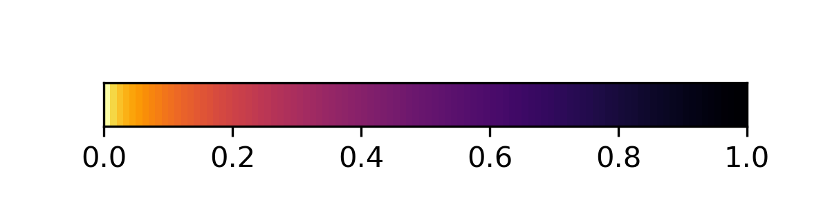
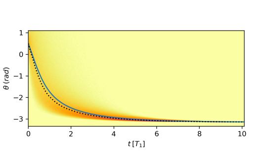
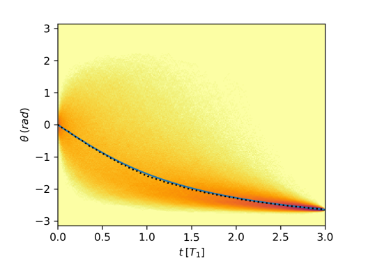
Figure 8: We compare ideal (pure–state) simulations against OPs generated by (70), between a few boundary conditions. All times ($x$–axes) are expressed in units of $T_{1}$, and all cases shown use $\Omega=0$. We plot the density of trajectories initialized at a given state $\vartheta_{i}$, and post–selected to within $\vartheta_{f}\pm 0.01$ at the final time on each plot; the density scale, which is normalized between the initial and final timesteps, is shown on the accompanying colorbar. The “experimental MLP” extracted from the post–selected SQTs, as described in sec. B, is shown over the density in dotted black, while the corresponding curve derived from the stochastic Hamiltonian (70) is shown in solid blue. In (a), we use $\vartheta_{i}=\tfrac{1}{2}$, and $\vartheta_{f}=-\pi+0.01$ at $T=10.1T_{1}$ (the post–selection window keeps SQTs which satisfy $\vartheta(10.1)\in[-\pi,-\pi+0.02]$). These boundary conditions are chosen such that the MLP shown approximately follows the separatrix in Fig. 6 from a state near $\left|e\right\rangle$, over the excited state, before decaying towards $\left|g\right\rangle$. In (b), we look at a somewhat less likely case, where trajectories are initialized at $\vartheta_{i}=0$ (the excited state $\left|e\right\rangle$), and the post–selection is applied at $\vartheta_{f}=-\pi+\tfrac{1}{2}$ at $T=3T_{1}$; so we are looking at anomalously slow decay, which is still hovering a bit above the ground state $\left|g\right\rangle$ after several decay times. We note that we have excellent agreement between the theoretical and numerical MLPs. It is also apparent that paths which dip “below” our chosen $\vartheta_{f}$ and then rise back to it are exceedingly rare; there are far more events in this PSSE which decayed partially to the “wrong” side of the Bloch sphere at early times and then came back over $\left|e\right\rangle$ to meet the final boundary condition.

Our expectation in deriving most–likely paths (MLPs) is that, in typical cases, they should correspond approximately to a highest–probability peak in the post–selected sub–ensemble of trajectories connecting an initial and final state (see comments below about some of the subtleties, however). Our aim here is to describe the procedure by which we approximate this concept in extracting a MLP from simulated SQTs or data, and show by example that such results are in good correspondence with those given by the CDJ optimization (see Sec. VI.2.1). This has been performed in a variety of cases elsewhere Weber et al. (2014); Naghiloo et al. (2017); Lewalle et al. (2018), and we here describe and perform the requisite analysis for solutions of (70) and the corresponding simulation.

We generically suppose that we are given a simulated ensemble of SQTs $\{{\rho(t)}\}$, initialized at a particular $\rho_{0}$; such trajectories are necessarily sampled over some small but discreet timestep $dt$, consistent with the simulation procedures described in the main body of the text above. We describe the numerical manipulations we perform on such a set of $\{{\rho(t)}\}$ to extract an “experimental MLP” which may be compared directly with theory. These go as follows:

1. We begin by imposing the final boundary condition, i.e. we post–select on the desired $\rho_{T}$, at a later time $T$. This means that we must pick a distance measure $D(\rho_{1},\rho_{2})$ between quantum states (e.g. fidelity, Bures distance, or similar), and keep the sub–ensemble for which $D(\rho(t=T),\rho_{T})\leq W$, where $W$ is some small widow or allowed tolerance about the chosen final state. We’ll call the post–selected sub–ensemble (PSSE) $\{\rho(t)\}_{ps}$; this is, by construction, the set of trajectories which connect $\rho_{0}$ to $\rho_{T}$.

2. A simple intuition about the meaning of the MLP is that it should follow a densest cluster of trajectories in $\{\rho(t)\}_{ps}$; in order to approximate this concept of a “densest cluster” numerically, we must rank each SQT in $\{\rho(t)\}_{ps}$ according to its distance to all other SQTs in $\{\rho(t)\}_{ps}$. It is useful to construct a matrix of elements $\mathfrak{D}_{nm}$, where $n$ and $m$ are indices which run over the SQTs in $\{\rho(t)\}_{ps}$; we write

   $$\mathfrak{D}_{nm}=\sum_{k}D(\rho_{n,k},\rho_{m,k}),$$ (82)

   where the sum over $k$ runs over all the timesteps between $t=0$ and $t=T$. The matrix $\mathfrak{D}$ will be symmetric as long as the distance measure $D$ is symmetric (we strongly discourage the use of any asymmetric distance measures for our present purposes). Then each SQT can be assigned a distance score relative to all other elements of $\{\rho(t)\}_{ps}$ according to $\bar{\mathfrak{D}}_{n}=\sum_{m}\mathfrak{D}_{nm}$, where a relatively smaller value of $\bar{\mathfrak{D}}_{n}$ indicates that trajectory $n$ of is closer to other trajectories in the post–selected set. These distances scores thus allow us to rank all of the trajectories in the PSSE.

3. The final step in the procedure is a simple average; we take the the closest–clustered 5%-10% of trajectories in $\{\rho(t)\}_{ps}$, (those with the smallest 5%-10% of $\bar{\mathfrak{D}}_{n}$), and average them. The idea is that this approximates the smooth curve following the densest cluster of SQTs in $\{\rho(t)\}_{ps}$.

We apply this procedure, and compare with the analytic solutions to (70), for a few selected boundary conditions, in Fig. 8.

We close with a few remarks about the procedure we have just described. We lack a formal proof that the numerical procedure just outlined necessarily always converges to the optimization we perform by the CDJ path integral method Chantasri et al. (2013). We nonetheless see in Fig. 8 that the present case continues to support the agreement between SQTs (from either simulation, or real data) and OPs, which have been successfully compared in many other scenarios as well Weber et al. (2014); Naghiloo et al. (2017); Lewalle et al. (2018). An important feature of the numerical procedure we have described is that it ranks trajectories by considering their entire evolution connecting $\mathbf{q}_{i}$ and $\mathbf{q}_{f}\tilde{\pm}W$, rather than looking for some piecewise optimization, or explicitly following a peak trajectory density at particular times. This reflects the character of the variational approach we have used in the theory; invoking $\delta\mathcal{S}=0$ leads to an optimization over an entire trajectory duration. While in many simple cases some piecewise numerical optimization could get us similar results, we would expect this simplified picture to fail in other cases, as it makes a substantial conceptual departure from the theory we want these numerics to match. In terms of practical considerations, we point out that the “experimental MLP” procedure above leads to an attrition in the number of SQTs used at each step, first due to post–selection, and then due to the ranking procedure. In order to obtain smooth results, it is necessary that at least several hundred SQTs make it into the final, most–closely clustered group which are averaged in step 3 above. The number of trajectories before post–selection, the size of the post–selection window, and the overall probability for trajectories to reach the desired final state, all play a role in these final numbers. The finer the post–selection window, the more initial trajectories are required at the beginning in order to obtain smooth results. Post–selections on very rare events may be prohibitively difficult to verify in practice, simply due to the overwhelming amount of data that would need to be collected / generated in order to have an appropriate number of SQTs in the PSSE.

References

- Einstein (1916) Albert Einstein, “Strahlungs-Emission und Absorption nach der Quantentheorie,” Deutsche Physikalische Gesellschaft 18 (1916).
- Dirac (1927) Paul A. M. Dirac, “The quantum theory of the emission and absorption of radiation,” Proceedings of the Royal Society A 114 (1927).
- Weisskopf and Wigner (1930) V. Weisskopf and E. Wigner, “Berechnung der natürlichen linienbreite auf grund der diracschen lichttheorie,” Zeitschrift für Physik 63, 54–73 (1930).
- Mollow (1969) B. R. Mollow, “Power spectrum of light scattered by two-level systems,” Phys. Rev. 188, 1969–1975 (1969).
- Ackerhalt et al. (1973) Jay R. Ackerhalt, Peter L. Knight, and Joseph H. Eberly, “Radiation reaction and radiative frequency shifts,” Phys. Rev. Lett. 30, 456–460 (1973).
- Kimble and Mandel (1976) H. J. Kimble and L. Mandel, “Theory of resonance fluorescence,” Phys. Rev. A 13, 2123–2144 (1976).
- Milonni (1984) P. W. Milonni, “Why spontaneous emission?” American Journal of Physics 52, 340–343 (1984).
- Haroche and Kleppner (1989) Serge Haroche and Daniel Kleppner, “Cavity quantum electrodynamics,” Physics Today 42, 24 (1989).
- Carmichael (1993) H. J. Carmichael, An Open Systems Approach to Quantum Optics (Springer, Berlin, 1993).
- Gardiner and Zoller (2004) C. W. Gardiner and P. Zoller, Quantum Noise: A Handbook of Markovian and Non-Markovian Quantum Stochastic Methods with Applications to Quantum Optics (Springer, 2004).
- Percival (1998) I. C. Percival, Quantum State Diffusion (Cambridge University Press, 1998).
- Wiseman and Milburn (2010) H. M. Wiseman and G. J. Milburn, Quantum measurement and control (Cambridge University Press, 2010).
- Barchielli and Gregoratti (2009) A. Barchielli and M. Gregoratti, Quantum trajectories and measurements in continuous time (Springer-Verlag Berlin Heidelberg, 2009).
- Jacobs (2014) Kurt Jacobs, Quantum Measurement Theory and its Applications (Cambridge University Press, 2014).
- Gisin (1984) N. Gisin, “Quantum measurements and stochastic processes,” Phys. Rev. Lett. 52, 1657–1660 (1984).
- Barchielli (1986) Alberto Barchielli, “Measurement theory and stochastic differential equations in quantum mechanics,” Phys. Rev. A 34, 1642–1649 (1986).
- Caves and Milburn (1987) Carlton M. Caves and G. J. Milburn, “Quantum-mechanical model for continuous position measurements,” Phys. Rev. A 36, 5543–5555 (1987).
- Diósi (1988) L. Diósi, “Continuous quantum measurement and Itô formalism,” Physics Letters A 129, 419 – 423 (1988).
- Gisin and Cibils (1992) N. Gisin and M. B. Cibils, “Quantum diffusions, quantum dissipation and spin relaxation,” Journal of Physics A: Mathematical and General 25, 5165–5176 (1992).
- Gisin and Percival (1992) N. Gisin and I. C. Percival, “The quantum-state diffusion model applied to open systems,” Journal of Physics A: Mathematical and General 25, 5677–5691 (1992).
- Wiseman and Milburn (1993a) H. M. Wiseman and G. J. Milburn, “Quantum theory of optical feedback via homodyne detection,” Phys. Rev. Lett. 70, 548–551 (1993a).
- Wiseman and Milburn (1993b) H. M. Wiseman and G. J. Milburn, “Quantum theory of field-quadrature measurements,” Phys. Rev. A 47, 642–662 (1993b).
- Wiseman and Milburn (1993c) H. M. Wiseman and G. J. Milburn, “Interpretation of quantum jump and diffusion processes illustrated on the bloch sphere,” Phys. Rev. A 47, 1652–1666 (1993c).
- Wiseman (1996) H. M. Wiseman, “Quantum trajectories and quantum measurement theory,” Quantum and Semiclassical Optics: Journal of the European Optical Society Part B 8, 205–222 (1996).
- Brun (2002) Todd A. Brun, “A simple model of quantum trajectories,” American Journal of Physics 70, 719 (2002).
- Gough and Sobolev (2004) John Gough and Andrei Sobolev, “Continuous measurement of canonical observables and limit stochastic Schrödinger equations,” Phys. Rev. A 69, 032107 (2004).
- Jacobs and Steck (2006) Kurt Jacobs and Daniel A. Steck, “A straightforward introduction to continuous quantum measurement,” Contemporary Physics 47, 279–303 (2006).
- Clerk et al. (2010) A. A. Clerk, M. H. Devoret, S. M. Girvin, Florian Marquardt, and R. J. Schoelkopf, “Introduction to quantum noise, measurement, and amplification,” Rev. Mod. Phys. 82, 1155–1208 (2010).
- Santos and Carvalho (2011) M. F. Santos and A. R. R. Carvalho, “Observing different quantum trajectories in cavity QED,” EPL (Europhysics Letters) 94, 64003 (2011).
- Gough et al. (2012) John E. Gough, Matthew R. James, Hendra I. Nurdin, and Joshua Combes, “Quantum filtering for systems driven by fields in single-photon states or superposition of coherent states,” Phys. Rev. A 86, 043819 (2012).
- Jordan (2013) Andrew N. Jordan, “Quantum physics: Watching the wavefunction collapse,” Nature 502, 177–178 (2013).
- Chantasri et al. (2013) A. Chantasri, J. Dressel, and A. N. Jordan, “Action principle for continuous quantum measurement,” Phys. Rev. A 88, 042110 (2013).
- Bolund and Mølmer (2014) Anders Bolund and Klaus Mølmer, “Stochastic excitation during the decay of a two-level emitter subject to homodyne and heterodyne detection,” Phys. Rev. A 89, 023827 (2014).
- Chantasri and Jordan (2015) Areeya Chantasri and Andrew N. Jordan, “Stochastic path-integral formalism for continuous quantum measurement,” Phys. Rev. A 92, 032125 (2015).
- Korotkov (2016) Alexander N. Korotkov, “Quantum Bayesian approach to circuit QED measurement with moderate bandwidth,” Phys. Rev. A 94, 042326 (2016).
- Gross et al. (2018) Jonathan A. Gross, Carlton M. Caves, Gerard J. Milburn, and Joshua Combes, “Qubit models of weak continuous measurements: Markovian conditional and open-system dynamics,” Quantum Science and Technology 3, 024005 (2018).
- Gough (2018a) John E. Gough, “An introduction to quantum filtering,” arXiv:1804.09086 (2018a).
- Gough (2018b) John E. Gough, “The Gisin-Percival stochastic Schrödinger equation from standard quantum filtering theory,” Journal of Mathematical Physics 59, 043509 (2018b).
- Gough (2019) John E. Gough, “How to estimate past measurement interventions on a quantum system undergoing continuous monitoring,” arXiv:1904.06364 (2019).
- Gough (2020) John E. Gough, “The collapse before a quantum jump transition,” Reports on Mathematical Physics 85, 69 – 76 (2020).
- Crowder et al. (2020) Gavin Crowder, Howard Carmichael, and Stephen Hughes, “Quantum trajectory theory of few-photon cavity-qed systems with a time-delayed coherent feedback,” Phys. Rev. A 101, 023807 (2020).
- Gisin et al. (1993) N. Gisin, P. L. Knight, I. C. Percival, R. C. Thompson, and D. C. Wilson, “Quantum state diffusion theory and a quantum jump experiment,” 40, 1663–1671 (1993).
- Gambetta et al. (2008) Jay Gambetta, Alexandre Blais, M. Boissonneault, A. A. Houck, D. I. Schuster, and S. M. Girvin, “Quantum trajectory approach to circuit QED: Quantum jumps and the Zeno effect,” Phys. Rev. A 77, 012112 (2008).
- Murch et al. (2013) K. W. Murch, S. J. Weber, C. Macklin, and I. Siddiqi, “Observing single quantum trajectories of a superconducting quantum bit,” Nature 502, 211 (2013).
- Weber et al. (2014) S. J. Weber, A. Chantasri, J. Dressel, A. N. Jordan, K. W. Murch, and I. Siddiqi, “Mapping the optimal route between two quantum states,” Nature 511, 570 (2014).
- Hacohen-Gourgy et al. (2016) S. Hacohen-Gourgy, L. S. Martin, E. Flurin, V. V. Ramasesh, K. B. Whaley, and I. Siddiqi, “Dynamics of simultaneously measured non-commuting observables,” Nature 538, 491 (2016).
- Lewalle et al. (2017) Philippe Lewalle, Areeya Chantasri, and Andrew N. Jordan, “Prediction and characterization of multiple extremal paths in continuously monitored qubits,” Phys. Rev. A 95, 042126 (2017).
- Dressel et al. (2017) Justin Dressel, Areeya Chantasri, Andrew N. Jordan, and Alexander N. Korotkov, “Arrow of time for continuous quantum measurement,” Phys. Rev. Lett. 119, 220507 (2017).
- Manikandan and Jordan (2019) Sreenath K. Manikandan and Andrew N. Jordan, “Time reversal symmetry of generalized quantum measurements with past and future boundary conditions,” Quantum Studies: Mathematics and Foundations 6, 241 (2019).
- Lewalle et al. (2018) Philippe Lewalle, John Steinmetz, and Andrew N. Jordan, “Chaos in continuously monitored quantum systems: An optimal-path approach,” Phys. Rev. A 98, 012141 (2018).
- Manikandan et al. (2019) Sreenath K. Manikandan, Cyril Elouard, and Andrew N. Jordan, “Fluctuation theorems for continuous quantum measurements and absolute irreversibility,” Phys. Rev. A 99, 022117 (2019).
- Patti et al. (2017) Taylor Lee Patti, Areeya Chantasri, Luis Pedro García-Pintos, Andrew N. Jordan, and Justin Dressel, “Linear feedback stabilization of a dispersively monitored qubit,” Phys. Rev. A 96, 022311 (2017).
- Hacohen-Gourgy et al. (2018) S. Hacohen-Gourgy, L. P. García-Pintos, L. S. Martin, J. Dressel, and I. Siddiqi, “Incoherent qubit control using the quantum Zeno effect,” Phys. Rev. Lett. 120, 020505 (2018).
- Minev et al. (2019) Z. K. Minev, S. O. Mundhada, S. Shankar, P. Reinhold, R. Gutierrez-Jauregui, R. J. Schoelkopf, M. Mirrahimi, H. J. Carmichael, and M. H. Devoret, “To catch and reverse a quantum jump mid-flight,” Nature 570, 200 (2019).
- Nielsen and Chuang (2000) M. A. Nielsen and I. L. Chuang, Quantum Computation and Quantum Information (Cambridge University Press, 2000).
- von Neumann (1932) J. von Neumann, Mathematical Foundations of Quantum Mechanics (Springer, 1932).
- Haroche and Raimond (2006) Serge Haroche and Jean-Michel Raimond, Exploring the Quantum: Atoms, Cavities, and Photons (Oxford Graduate Texts) (Oxford University Press, 2006).
- Aharonov et al. (1988) Yakir Aharonov, David Z. Albert, and Lev Vaidman, “How the result of a measurement of a component of the spin of a spin-1/2 particle can turn out to be 100,” Phys. Rev. Lett. 60, 1351–1354 (1988).
- Tamir and Cohen (2013) Boaz Tamir and Eliahu Cohen, “Introduction to weak measurements and weak values,” Quanta 2, 7–17 (2013).
- Fuchs and Peres (1996) Christopher A. Fuchs and Asher Peres, “Quantum-state disturbance versus information gain: Uncertainty relations for quantum information,” Phys. Rev. A 53, 2038–2045 (1996).
- Fuchs and Jacobs (2001) Christopher A. Fuchs and Kurt Jacobs, “Information-tradeoff relations for finite-strength quantum measurements,” Phys. Rev. A 63, 062305 (2001).
- Oreshkov and Brun (2005) Ognyan Oreshkov and Todd A. Brun, “Weak measurements are universal,” Phys. Rev. Lett. 95, 110409 (2005).
- Leuchs (1988) Gerd Leuchs, “Squeezing the quantum fluctuations of light,” Contemporary Physics 29, 299–314 (1988).
- Silberhorn (2007) Christine Silberhorn, “Detecting quantum light,” Contemporary Physics 48, 143–156 (2007).
- Campagne-Ibarcq et al. (2014) P. Campagne-Ibarcq, L. Bretheau, E. Flurin, A. Auffèves, F. Mallet, and B. Huard, “Observing interferences between past and future quantum states in resonance fluorescence,” Phys. Rev. Lett. 112, 180402 (2014).
- Jordan et al. (2015) Andrew N. Jordan, Areeya Chantasri, Pierre Rouchon, and Benjamin Huard, “Anatomy of fluorescence: Quantum trajectory statistics from continuously measuring spontaneous emission,” Quantum Studies: Math. and Found. 3, 237 (2015).
- Campagne-Ibarcq et al. (2016a) P. Campagne-Ibarcq, P. Six, L. Bretheau, A. Sarlette, M. Mirrahimi, P. Rouchon, and B. Huard, “Observing quantum state diffusion by heterodyne detection of fluorescence,” Phys. Rev. X 6, 011002 (2016a).
- Campagne-Ibarcq et al. (2016b) P. Campagne-Ibarcq, S. Jezouin, N. Cottet, P. Six, L. Bretheau, F. Mallet, A. Sarlette, P. Rouchon, and B. Huard, “Using spontaneous emission of a qubit as a resource for feedback control,” Phys. Rev. Lett. 117, 060502 (2016b).
- Naghiloo et al. (2016) M. Naghiloo, N. Foroozani, D. Tan, A. Jadbabaie, and K. W. Murch, “Mapping quantum state dynamics in spontaneous emission,” Nature Communications 7, 11527 (2016).
- Naghiloo et al. (2017) M. Naghiloo, D. Tan, P. M. Harrington, P. Lewalle, A. N. Jordan, and K. W. Murch, “Quantum caustics in resonance-fluorescence trajectories,” Phys. Rev. A 96, 053807 (2017).
- Tan et al. (2017) D. Tan, N. Foroozani, M. Naghiloo, A. H. Kiilerich, K. Mølmer, and K. W. Murch, “Homodyne monitoring of postselected decay,” Phys. Rev. A 96, 022104 (2017).
- Naghiloo et al. (2020) M. Naghiloo, D. Tan, P. M. Harrington, J. J. Alonso, E. Lutz, A. Romito, and K. W. Murch, “Heat and work along individual trajectories of a quantum bit,” Phys. Rev. Lett. 124, 110604 (2020).
- Ficheux et al. (2018) Q. Ficheux, S. Jezouin, Z. Leghtas, and B. Huard, “Dynamics of a qubit while simultaneously monitoring its relaxation and dephasing,” Nat. Comm. 9, 1926 (2018).
- Ficheux (2018) Quentin Ficheux, “Quantum trajectories with incompatible decoherence channels,” Dissertation, École normale supérieure—Paris (2018).
- Naghiloo (2019) Mahdi Naghiloo, “Introduction to experimental quantum measurement with superconducting qubits,” arXiv 1904.09291 (2019).
- Areeya Chantasri (2016) Areeya Chantasri, “Stochastic path integral formalism for continuous quantum measurement,” PhD Dissertation, University of Rochester (2016).
- Bergeal et al. (2010) N. Bergeal, F. Schackert, M. Metcalfe, R. Vijay, V. E. Manucharyan, L. Frunzio, D. E. Prober, R. J. Schoelkopf, S. M. Girvin, and M. H. Devoret, “Phase-preserving amplification near the quantum limit with a Josephson ring modulator,” Nature 465, 6 (2010).
- Emmanuel Flurin (2014) Emmanuel Flurin, “The Josephson Mixer: A Swiss army knife for microwave quantum optics,” PhD Dissertation, Ecole Normale Supérieure, Paris (2014).
- Roy and Devoret (2016) Ananda Roy and Michel Devoret, “Introduction to parametric amplification of quantum signals with Josephson circuits,” Comptes Rendus Physique 17, 740 – 755 (2016).
- Breuer et al. (1997) Heinz-Peter Breuer, Bernd Kappler, and Francesco Petruccione, “Stochastic wave-function approach to the calculation of multitime correlation functions of open quantum systems,” Phys. Rev. A 56, 2334 (1997).
- Cohen-Tannoudji et al. (1998) Claude Cohen-Tannoudji, Jacques Dupont-Roc, and Gilbert Grynberg, Atom—Photon Interactions (1998).
- Breuer and Petruccione (2002) H.-P. Breuer and F. Petruccione, The Theory of Open Quantum Systems (Oxford University Press, 2002).
- Murch et al. (2012) K. W. Murch, U. Vool, D. Zhou, S. J. Weber, S. M. Girvin, and I. Siddiqi, “Cavity-Assisted Quantum Bath Engineering,” Phys. Rev. Lett. 109, 183602 (2012).
- Carmichael (1999) Howard J. Carmichael, Statistical Methods in Quantum Optics I: Master Equations and Fokker–Planck Equations (Springer–Verlag Berlin Heidelberg, 1999).
- (85) R. P. Feynman, “The Brownian Movement,” in The Feynman Lectures on Physics, Volume I (CalTech) Chap. 41.
- Gardiner (2004) C. W. Gardiner, Handbook of Stochastic Methods for Physics, Chemistry and the Natural Sciences (Springer, 2004).
- Kloeden and Platen (1992) Peter E. Kloeden and Eckhard Platen, Numerical Solution of Stochastic Differential Equations (Springer, 1992).
- Press et al. (1988) William H. Press, Brian P. Flannery, Saul A. Teukolsky, and William T. Vetterling, Numerical Recipes in C (Cambridge University Press, 1988).
- Rouchon and Ralph (2015) Pierre Rouchon and Jason F. Ralph, “Efficient quantum filtering for quantum feedback control,” Phys. Rev. A 91, 012118 (2015).
- Quijandría et al. (2018) Fernando Quijandría, Ingrid Strandberg, and Göran Johansson, “Steady-State Generation of Wigner-Negative States in One-Dimensional Resonance Fluorescence,” Phys. Rev. Lett. 121, 263603 (2018).
- Tyc and Sanders (2004) Tomáš Tyc and Barry C. Sanders, “Operational formulation of homodyne detection,” Journal of Physics A: Mathematical and General 37, 7341 (2004).
- Dziarmaga et al. (2004) Jacek Dziarmaga, Diego A. R. Dalvit, and Wojciech H. Zurek, “Conditional quantum dynamics with several observers,” Phys. Rev. A 69, 022109 (2004).
- Harrington et al. (2019) P. M. Harrington, D. Tan, M. Naghiloo, and K. W. Murch, “Characterizing a statistical arrow of time in quantum measurement dynamics,” Phys. Rev. Lett. 123, 020502 (2019).
- Lewalle et al. (2019a) Philippe Lewalle, Cyril Elouard, Sreenath K. Manikandan, Xiao-Feng Qian, Joseph H. Eberly, and Andrew N. Jordan, “Entanglement of a pair of quantum emitters under continuous fluorescence measurements,” arXiv: 1910.01206 (2019a).
- Kuramochi et al. (2013) Yui Kuramochi, Yu Watanabe, and Masahito Ueda, “Simultaneous continuous measurement of photon-counting and homodyne detection on a free photon field: dynamics of state reduction and the mutual influence of measurement backaction,” Journal of Physics A: Mathematical and Theoretical 46, 425303 (2013).
- Guevara and Wiseman (2015) Ivonne Guevara and Howard Wiseman, “Quantum state smoothing,” Phys. Rev. Lett. 115, 180407 (2015).
- Chantasri et al. (2019) Areeya Chantasri, Ivonne Guevara, and Howard M Wiseman, “Quantum state smoothing: why the types of observed and unobserved measurements matter,” New Journal of Physics 21, 083039 (2019).
- (98) Ivonne Guevara and Howard M. Wiseman, “Completely positive quantum trajectories with applications to quantum state smoothing,” arXiv:1909.12455 .
- Hawking (1985) S. W. Hawking, “Arrow of time in cosmology,” Phys. Rev. D 32, 2489–2495 (1985).
- Maccone (2009) Lorenzo Maccone, “Quantum solution to the arrow-of-time dilemma,” Phys. Rev. Lett. 103, 080401 (2009).
- Lebowitz (1993) Joel L. Lebowitz, “Boltzmann’s entropy and time’s arrow,” Physics Today 46, 32 (1993).
- Jordan and Korotkov (2010) Andrew N. Jordan and Alexander N. Korotkov, “Uncollapsing the wavefunction by undoing quantum measurements,” Contemporary Physics 51, 125–147 (2010).
- Korotkov and Jordan (2006) Alexander N. Korotkov and Andrew N. Jordan, “Undoing a weak quantum measurement of a solid-state qubit,” Phys. Rev. Lett. 97, 166805 (2006).
- Chernyak et al. (2006) Vladimir Y. Chernyak, Michael Chertkov, and Christopher Jarzynski, “Path-integral analysis of fluctuation theorems for general Langevin processes,” Journal of Statistical Mechanics: Theory and Experiment 2006, P08001 (2006).
- Tan et al. (2015) D. Tan, S. J. Weber, I. Siddiqi, K. Mølmer, and K. W. Murch, “Prediction and retrodiction for a continuously monitored superconducting qubit,” Phys. Rev. Lett. 114, 090403 (2015).
- Cottet et al. (2017) Nathanaël Cottet, Sébastien Jezouin, Landry Bretheau, Philippe Campagne-Ibarcq, Quentin Ficheux, Janet Anders, Alexia Auffèves, Rémi Azouit, Pierre Rouchon, and Benjamin Huard, “Observing a quantum Maxwell demon at work,” PNAS 114, 7561–7564 (2017).
- Elouard et al. (2017a) Cyril Elouard, David A. Herrera-Martí, Maxime Clusel, and Alexia Auffèves, “The role of quantum measurement in stochastic thermodynamics,” NPJ Quantum Information 3, 9 (2017a).
- Elouard et al. (2017b) Cyril Elouard, David Herrera-Martí, Benjamin Huard, and Alexia Auffèves, “Extracting Work from Quantum Measurement in Maxwell’s Demon Engines,” Phys. Rev. Lett. 118, 260603 (2017b).
- Elouard and Jordan (2018) Cyril Elouard and Andrew N. Jordan, “Efficient quantum measurement engines,” Phys. Rev. Lett. 120, 260601 (2018).
- Masuyama et al. (2018) Y. Masuyama, K. Funo, Y. Murashita, A. Noguchi, S. Kono, Y. Tabuchi, R. Yamazaki, M. Ueda, and Y. Nakamura, “Information-to-work conversion by Maxwell’s demon in a superconducting circuit quantum electrodynamical system,” Nature Communications 9, 1291 (2018).
- Monsel et al. (2018) Juliette Monsel, Cyril Elouard, and Alexia Auffèves, “An autonomous quantum machine to measure the thermodynamic arrow of time,” npj Quantum Information 4, 59 (2018).
- Monsel et al. (2019) Juliette Monsel, Marco Fellous-Asiani, Benjamin Huard, and Alexia Auffèves, “A coherent quantum engine based on bath and battery engineering,” arXiv:1907.00812 (2019).
- Mohammady et al. (2019) M. H. Mohammady, A. Auffèves, and J. Anders, “Energetic footprints of irreversibility in the quantum regime,” arXiv:1907.06559 (2019).
- Wang and Wiseman (2001) Jin Wang and H. M. Wiseman, “Feedback-stabilization of an arbitrary pure state of a two-level atom,” Phys. Rev. A 64, 063810 (2001).
- Murch et al. (2015) Kater W. Murch, Rajamani Vijay, and Irfan Siddiqi, “Weak measurement and feedback in superconducting quantum circuits,” arXiv:1507.04617v2 (2015).
- Atalaya et al. (2018) Juan Atalaya, Shay Hacohen-Gourgy, Leigh S. Martin, Irfan Siddiqi, and Alexander N. Korotkov, “Multitime correlators in continuous measurement of qubit observables,” Phys. Rev. A 97, 020104 (2018).
- Mascarenhas et al. (2011) Eduardo Mascarenhas, Daniel Cavalcanti, Vlatko Vedral, and Marcelo França Santos, “Physically realizable entanglement by local continuous measurements,” Phys. Rev. A 83, 022311 (2011).
- Santos et al. (2012) M. F. Santos, M. Terra Cunha, R. Chaves, and A. R. R. Carvalho, “Quantum computing with incoherent resources and quantum jumps,” Phys. Rev. Lett. 108, 170501 (2012).
- Lewalle et al. (2019b) Philippe Lewalle, Cyril Elouard, Sreenath K. Manikandan, Xiao-Feng Qian, Joseph H. Eberly, and Andrew N. Jordan, “Diffusive entanglement generation by continuous homodyne monitoring of spontaneous emission,” arXiv: 1910.01204 (2019b).
- Yu and Eberly (2004) Ting Yu and J. H. Eberly, “Finite-time disentanglement via spontaneous emission,” Phys. Rev. Lett. 93, 140404 (2004).
- Mintert et al. (2005) Florian Mintert, André R. R. Carvalho, Marek Kuś, and Andreas Buchleitner, “Measures and dynamics of entangled states,” Physics Reports 415, 207 – 259 (2005).
- Viviescas et al. (2010) Carlos Viviescas, Ivonne Guevara, André R. R. Carvalho, Marc Busse, and Andreas Buchleitner, “Entanglement dynamics in open two-qubit systems via diffusive quantum trajectories,” Phys. Rev. Lett. 105, 210502 (2010).
- Mascarenhas et al. (2010) Eduardo Mascarenhas, Breno Marques, Marcelo Terra Cunha, and Marcelo França Santos, “Continuous quantum error correction through local operations,” Phys. Rev. A 82, 032327 (2010).
- Carvalho and Santos (2011) André R. R. Carvalho and Marcelo França Santos, “Distant entanglement protected through artificially increased local temperature,” New Journal of Physics 13, 013010 (2011).
- Wiseman (2015) Howard M. Wiseman, “Death by experiment for local realism,” Nature 526, 649 (2015).