Critical Decisions for Asset Allocation via Penalized Quantile Regression

Abstract

We extend the analysis of investment strategies derived from penalized quantile regression models, introducing alternative approaches to improve state–of–art asset allocation rules. First, we use a post–penalization procedure to deal with overshrinking and concentration issues. Second, we investigate whether and to what extent the performance changes when moving from convex to nonconvex penalty functions. Third, we compare different methods to select the optimal tuning parameter which controls the intensity of the penalization. Empirical analyses on real–world data show that these alternative methods outperform the simple LASSO. This evidence becomes stronger when focusing on the extreme risk, which is strictly linked to the quantile regression method.

Keywords: Penalized quantile regression $\cdot$ Portfolio optimization $\cdot$ Performance evaluation

1 Introduction

Recent financial crises have shown the impact of extreme losses on the overall system, highlighting the need to design better investment strategies and risk management policies to minimize or predict more accurately the effects of tail events. Therefore, the focus has begun to shift toward pessimistic asset allocation strategies, designed to minimize measures of extreme risk, going beyond the classical mean–variance theory pioneered by Markowitz (1952). Among the various measures of extreme risk studied in the theoretical and empirical literature, the expected shortfall (ES) introduced by the seminal works of Rockafellar and Uryasev (2000) and Acerbi and Tasche (2002) has received a relevant attention (see, among many others, Yamai and Yoshiba (2005), Chen (2008), Assa (2015), Gijbels and Herrmann (2018), Kratz et al. (2018) and Patton et al. (2019)). This is mainly due to the fact that the ES has useful mathematical and statistical properties, being a coherent risk measure according to Artzner et al. (1999).

Several works used the ES as a target measure in portfolio optimization problems (see, e.g., Gilli and Këllezi (2002) and Ciliberti et al. (2007)). Bassett et al. (2004) showed that it is possible to efficiently minimize the ES of a given portfolio using the quantile regression method introduced by Koenker and Bassett (1978). Indeed, the coefficients of a quantile regression model, whose variables are computed from the returns yielded by the selected stocks, coincide with the weights of the portfolio with minimum ES. Financial portfolios are typically built using a large number of stocks to exploit the advantages arising from their diversification. On the other hand, the larger the portfolio dimensionality is, the larger the number of parameters to estimate. The resulting accumulation of estimation errors is then a critical issue, especially in terms of out–of–sample performance. Moreover, financial returns are typically highly correlated and the resulting portfolio weights turn out to be poorly determined, exhibiting a relevant variance.

In a context in which the optimal weights of a given portfolio are derived from regression models, regularization techniques have proven to be an effective tool to deal with the curse of dimensionality. For instance, Fastrich et al. (2015) showed that sparse portfolios derived from penalized regression models provide improvements in terms of a lower concentration and turnover. Giuzio and Paterlini (2018) highlighted the positive impact of regularized models on the portfolio performance during stressed market conditions. Kremer et al. (2018) used regularization techniques to minimize the risk in multi–factor portfolios. The studies cited above, as well as many others in the literature, used various penalty functions to regularize a given regression model. Among them, the $\ell_{1}$–norm penalty, leading to the Least Absolute Shrinkage and Selection Operator (LASSO) introduced by Tibshirani (1996), is one of the most commonly used penalization method in the financial literature (see, e.g., Brodie et al. (2009), DeMiguel et al. (2009), Fan et al. (2012) and Yen and Yen (2014)). In recent years, the LASSO has gained attention in the statistical literature not only when implemented on standard linear regressions but also on quantile regression models (see, e.g., Koenker (2005), Li and Zhu (2008) and Belloni and Chernozhukov (2011)). In contrast, applications of penalized quantile regression models to build asset allocation strategies are still limited.

In this study, we focus on Bonaccolto et al. (2018), who analyzed the performance of financial portfolios derived from quantile regression models including an $\ell_{1}$–norm penalty, highlighting the resulting improvements in terms of out–of–sample performance. However, the work of Bonaccolto et al. (2018) opened the door to further research, that we investigate in this study. An important research question is related to the use of the LASSO. Indeed, although the LASSO has many remarkable properties, it suffers from some limitations. For instance, it typically provides biased estimates, overshrinking the retained variables (see, e.g., Fan and Li (2001)). Under a financial viewpoint, this overshrinking causes a problematic consequence. Indeed, as highlighted by Bonaccolto et al. (2018), the asset having the role of response variable in the underlying regression model is typically overweighted. This raises problems in terms of portfolio concentration. In this study, we address this issue using a post–LASSO procedure, that is a well–known method in the financial econometrics literature. For instance, Hautsch et al. (2014) used a post–LASSO method to estimate pessimistic financial networks. Moreover, we also use nonconvex penalty functions, such as the Smoothly Clipped Absolute Deviation (SCAD) and the Minimax Concave Penalty (MCP), introduced, respectively, by Fan and Li (2001) and Zhang (2010), which have the oracle property as defined by Fan and Li (2001). Many works in the literature used nonconvex penalty functions in standard linear regression models to build financial portfolios (see, among others, Giuzio (2017)). Nevertheless, to the best of our knowledge, this is the first study in which a post–LASSO procedure and nonconvex penalty functions are used within a quantile regression model to design asset allocation strategies.

Another relevant point is related to the method we use to control the intensity of the penalization; that is, the optimal tuning parameter. Bonaccolto et al. (2018) used the data–driven method that Belloni and Chernozhukov (2011) developed for quantile regression models including an $\ell_{1}$–norm penalty. However, other selection methods are available in the literature. In this study, we also use a Bayesian Information Criterion (BIC) that Lee et al. (2014) designed for quantile regression models and the $K$–fold cross–validation, that is commonly used in applied machine learning, being flexible and easy to understand and implement (see, e.g., Hastie et al. (2009)). In contrast to the method of Belloni and Chernozhukov (2011), the BIC and the $K$–fold cross–validation are flexible to be used on any penalized quantile regression model, regardless of the specification of its penalty function. To the best of our knowledge, the BIC of Lee et al. (2014) and cross–validation techniques have never been tested in building financial portfolios from quantile regression models.

We evaluate the competing penalty functions and regularization parameter selection methods, as well as the opportunity of using a post–penalization procedure, by means of an extensive empirical analysis. The out–of–sample results highlight the significant improvements yielded by some of the resulting portfolios. Among them, we emphasize the outperformance of the rule in which we combine the post–LASSO procedure with the selection method of Belloni and Chernozhukov (2011). This evidence becomes stronger when focusing on the risk dimension, in terms of both standard deviation and expected shortfall of the out–of–sample portfolio returns. In particular, the latter acquires a central role in this study, as it represents the risk measure we minimize when estimating a quantile regression model. We also observe that nonconvex penalty functions often outperform the simple LASSO, providing then an additional valid alternative to state–of–art methods. Moreover, our proposal turns out to be an effective tool to deal with the portfolio concentration issues highlighted by Bonaccolto et al. (2018), mitigating the weight of the stock whose return represents the response variable in the underlying quantile regression model. Finally, our portfolio strategies are computationally efficient, providing then an advantageous tool for different financial agents, such as hedge funds, to improve the performance of their portfolios, while controlling the risk of incurring large losses during tail events.

The paper is structured as follows. Section 2 describes the penalized quantile regression models we estimate to build financial portfolios. Section 3 reports the details of the empirical set–up. Section 4 reports and discusses the main empirical results, whereas Section 5 concludes the paper.

2 Methods

Let $\textbf{r}_{t}=\left[r_{1,t}\;r_{2,t}\;\cdots\;r_{N,t}\right]$ be an $1\times N$ vector of returns yielded by $N$ assets that we observe at time $t$, for $t=1,...,T$. We also define an $1\times N$ vector of portfolio weights, denoted as $\textbf{w}=\left[w_{1}\;w_{2}\;\cdots\;w_{N}\right]$. We focus on portfolios satisfying the budget constraint, such that $\textbf{w}\left(\textbf{1}_{N}\right)^{\prime}=1$, where $\textbf{1}_{N}$ is an $1\times N$ unit vector. We then compute the portfolio return as $r_{p,t}=\textbf{r}_{t}\textbf{w}^{\prime}$, for $t=1,...,T$.

Following Fan et al. (2012), we can efficiently rewrite the return of a portfolio satisfying the budget constraint. For this purpose, we must select a reference index $s\in\{1,...,N\}$ and then define the variables $x_{s,t}=r_{s,t}$ and $x_{j,t}=x_{s,t}-r_{j,t}$, for $1\leq j\leq N$ and $j\neq s$. As a result, the return of this portfolio is defined as follows:

$$r_{p,t}=x_{s,t}-\sum_{\begin{subarray}{c}j=1\\ j\neq s\end{subarray}}^{N}w_{j}x_{j,t},$$ (1)

where the weight of the $s$–th asset is equal to $w_{s}=1-\sum_{\begin{subarray}{c}j=1\\ j\neq s\end{subarray}}^{N}w_{j}$ to satisfy the condition $\textbf{w}\left(\textbf{1}_{N}\right)^{\prime}=1$.

Bassett et al. (2004) introduced a method building on the quantile regression method (Koenker and Bassett, 1978) to minimize the expected shortfall (ES) at the level $\tau$ of a given portfolio, where $\tau$ takes low values, typically in the interval $(0,0.05]$ (see Acerbi and Tasche (2002), Rockafellar and Uryasev (2000) and Artzner et al. (1999) for a detailed description of the properties of the ES). Bonaccolto et al. (2018) studied the performance of large portfolios keeping the focus on the pessimistic asset allocation of Bassett et al. (2004). The number of parameters to estimate increases with $N$. The accumulation of estimation errors becomes then a critical issue when $N$ takes large values. Bonaccolto et al. (2018) dealt with the curse of dimensionality using the Least Absolute Shrinkage and Selection Operator (LASSO) introduced by Tibshirani (1996). In particular, by adding an $\ell_{1}$–norm penalty to the objective function of the standard quantile regression model, Bonaccolto et al. (2018) derived the portfolio weights from the following minimization problem:

$$\operatorname*{arg\,min}_{(\textbf{w}_{(-s)},\;\mu)\in\mathbb{R}^{N}}\frac{1}{T}\sum_{t=1}^{T}\rho_{\tau}\left(x_{s,t}-\sum_{\begin{subarray}{c}j=1\\ j\neq s\end{subarray}}^{N}w_{j}x_{j,t}-\mu\right)+\lambda\frac{\sqrt{\tau(1-\tau)}}{T}\sum_{\begin{subarray}{c}j=1\\ j\neq s\end{subarray}}^{N}\widehat{\sigma}_{j}|w_{j}|,$$ (2)

where $\rho_{\tau}(u)=u\left(\tau-\mathbb{I}_{\{u<0\}}\right)$ is the asymmetric loss function used by Koenker and Bassett (1978), $\mathbb{I}_{\{\cdot\}}$ is an indicator function which takes the value of one if the condition in $\{\cdot\}$ is true, the value of zero otherwise, $\textbf{w}_{(-s)}$ is the vector of the portfolio weights without $w_{s}$ (which is computed in a subsequent step as $w_{s}=1-\sum_{\begin{subarray}{c}j=1\\ j\neq s\end{subarray}}^{N}w_{j}$), $\widehat{\sigma}_{j}$ is the sample standard deviation of the variable $x_{j,t}$ and $\lambda>0$ is a tuning parameter.

The statistical properties of the penalized quantile regression model building on the minimization problem in (2) were widely studied by Belloni and Chernozhukov (2011). The tuning parameter $\lambda$ acquires a central role, as it controls the intensity of the penalization. Indeed, the greater $\lambda$ is, the sparser the solution derived from (2), with an increasing number of coefficients (the portfolio weights) which approach zero. Belloni and Chernozhukov (2011) introduced a data–driven method with optimal asymptotic properties to determine the optimal value of $\lambda$. This method requires to compute the following quantity:

$$\Lambda=T\operatorname*{max}_{\begin{subarray}{c}1\leq j\leq N\\ j\neq s\end{subarray}}\left|\frac{1}{T}\sum_{t=1}^{T}\left[\frac{x_{j,t}(\tau-\mathbb{I}_{\{e_{t}\leq\tau\}})}{\widehat{\sigma}_{j}\sqrt{\tau(1-\tau)}}\right]\right|,$$ (3)

where $e_{1},\cdots,e_{T}$ are i.i.d. uniform $(0,1)$ random variables.

We then estimate the empirical distribution function of $\Lambda$ by running $B$ iterations and compute the optimal value of $\lambda$ as follows:

$$\lambda^{\star}=c\cdot\Lambda(1-\beta|\textbf{X}),$$ (4)

where $\Lambda(1-\beta|\textbf{X})$ is the $(1-\beta)$–th quantile of $\Lambda$ conditional on the covariates $x_{j,t}$, for $1\leq j\leq N$ and $j\neq s$, whereas $c>1$ is a scalar parameter.

In sum, Bonaccolto et al. (2018) derived the weights of the portfolio with minimum ES at the level $\tau$ from the minimization problem in (2), where the optimal value of $\lambda$ is computed from (4). We label this strategy as LBCH, where L and BCH stand, respectively, for the LASSO and for the regularization parameter selection method of Belloni and Chernozhukov (2011).

The LASSO is one of the most commonly used penalization method in the statistical literature because it has important properties. Nevertheless, it also suffers from some limitations. For instance, it typically provides biased estimates, overshrinking the retained variables (see e.g., Fan and Li (2001)). As a result, when implementing the strategy LBCH, the $s$–th asset tends to be overweighted, as highlighted by Bonaccolto et al. (2018). Indeed, the $\ell_{1}$–norm penalizes the coefficients of the regressors in (2), shrinking the value of $\sum_{\begin{subarray}{c}j=1\\ j\neq s\end{subarray}}^{N}w_{j}$. This increases the value of $w_{s}$, being computed in a subsequent step (i.e., after minimizing the loss in (2)) as the complement of $\sum_{\begin{subarray}{c}j=1\\ j\neq s\end{subarray}}^{N}w_{j}$. Moreover, the coefficients derived from (2) are generally downwardly biased in finite samples (see Belloni and Chernozhukov (2011) and Hautsch et al. (2014)). In this study, we address this issue by using the post–LASSO procedure. This is a well–known method in the financial econometrics literature. For instance, Hautsch et al. (2014) used the post–LASSO rule to estimate pessimistic financial networks. However, to the best of our knowledge, this is the first study which uses the post–LASSO estimation to build financial portfolios from penalized (not only quantile) regression models.

Following Hautsch et al. (2014), we minimize in the first step the loss in (2) and discard the $j$–th regressor $x_{j,t}$ if its shrunken absolute coefficient is sufficiently close to zero; that is, if $|w_{j}|\leq\eta$, where $\eta$ is a given threshold. In contrast, we select the $D$ regressors (with $D\leq N-1$) with a relevant impact—the ones whose absolute coefficients satisfy the condition $|w_{j}|>\eta$, for $1\leq j\leq N$ and $j\neq s$. Given the set $\mathcal{D}=\{j_{1},\cdots,j_{D}\}\subset\{1,\cdots,N\}$, we define: i) the vector of the selected covariates as $\textbf{x}_{\mathcal{D},t}=\left[x_{j_{1},t}\;\cdots\;x_{j_{D},t}\right]$; and ii) the vector including their weights as $\textbf{w}_{\mathcal{D}}=\left[w_{j_{1}}\;\cdots\;w_{j_{D}}\right]$. In the second step, we compute the optimal weights of the selected assets from the following (nonpenalized) minimization problem:

$$\operatorname*{arg\,min}_{(\textbf{w}_{\mathcal{D}},\;\mu^{\star})\in\mathbb{R}^{(D+1)}}\frac{1}{T}\sum_{t=1}^{T}\rho_{\tau}\left(x_{s,t}-\textbf{x}_{\mathcal{D},t}\cdot(\textbf{w}_{\mathcal{D}})^{\prime}-\mu^{\star}\right),$$ (5)

whereas the coefficients of the regressors which do not appear in (5) (i.e., the ones we discard in the first step) are set to zero.

Therefore, in contrast to Bonaccolto et al. (2018), we use the LASSO as a selection variable tool only in the first step. Indeed, the portfolio weights are computed in the second step from the nonpenalized minimization problem in (5). The post–LASSO procedure provides improvements under both a statistical and a financial viewpoint. For example, as highlighted by Belloni and Chernozhukov (2011) and Hautsch et al. (2014), the post–LASSO method outperforms both the simple LASSO and the standard quantile regression, which suffer from overidentification problems. Moreover, we compute the portfolio weights without penalizing the coefficients in (5). As a result, we mitigate the complement of the sum $\sum_{d=1}^{D}w_{j_{d}}$; that is, the weight of the $s$–th asset. We label this strategy as PLBCH, where PL stands for post–LASSO, whereas BCH denotes the method of Belloni and Chernozhukov (2011) that we adopt to select the optimal value of $\lambda$ in the first step.

The asset allocation strategies described so far rely on the regularization parameter selection method of Belloni and Chernozhukov (2011). Nevertheless, other competing rules are available in the statistical literature. Therefore, it is interesting to compare these different approaches and assess whether and to what extent they affect the portfolio performance. The second selection method we consider in this study is the Bayesian Information Criterion (BIC) introduced by Lee et al. (2014). Lee et al. (2014) proposed a BIC for quantile regression models under the assumption that the error term $\epsilon_{t}=x_{s,t}-\textbf{x}_{\mathcal{D},t}\cdot(\widehat{\textbf{w}}_{\mathcal{D}})^{\prime}-\widehat{\mu}^{\star}$ has an asymmetric Laplace distribution with the following density function:

$$f(\epsilon_{t};\tau,\sigma)=\frac{\tau(1-\tau)}{\nu}\exp\left\{-\frac{\rho_{\tau}(\epsilon_{t})}{\nu}\right\},$$ (6)

where the maximum likelihood estimator of $\nu$ is defined as follows:

$$\widehat{\nu}=\frac{1}{T}\sum_{t=1}^{T}\rho_{\tau}\left(x_{s,t}-\textbf{x}_{\mathcal{D},t}\cdot(\widehat{\textbf{w}}_{\mathcal{D}})^{\prime}-\widehat{\mu}^{\star}\right),$$ (7)

whereas the coefficients $\widehat{\mu}^{\star}$ and $\widehat{\textbf{w}}_{\mathcal{D}}$ are obtained by minimizing the loss in (5).

Among the alternative specifications proposed by Lee et al. (2014), we adopt the following one:

$$BIC_{L}^{H}(\mathcal{D})=\log\left(2\sum_{t=1}^{T}\rho_{\tau}\left(x_{s,t}-\textbf{x}_{\mathcal{D},t}\cdot(\widehat{\textbf{w}}_{\mathcal{D}})^{\prime}-\widehat{\mu}^{\star}\right)\right)+|\mathcal{D}|\frac{\log T}{2T}C_{T},$$ (8)

where $|\mathcal{D}|$ is the cardinality of the set $\mathcal{D}=\{j_{1},\cdots,j_{D}\}$, whereas $C_{T}$ is a positive constant.

We choose $BIC_{L}^{H}(\mathcal{D})$ because it provides consistent results in high–dimensional problems (Lee et al., 2014). Again, we implement the post–LASSO procedure. In particular, we minimize the loss function in (2) by using a large grid of $\lambda$ values. For each value of $\lambda$, we then select the relevant regressors, including them in (5) to obtain the post–LASSO portfolio weights. Among the different solutions derived from (5), we choose the one providing the minimum $BIC_{L}^{H}$. We label this strategy as PLBIC because it combines the post–LASSO method with the BIC proposed by Lee et al. (2014).

The third selection method we use in this study is the $K$–fold cross–validation (CV$K$). It is commonly used in applied machine learning, being flexible and easy to implement (see, e.g., Hastie et al. (2009)). The $K$–fold cross–validation requires the following steps:

• we randomly divide our dataset into $K$ folds of (approximately) equal size;

• we use the first fold as the validation set, whereas the remaining ones form the training set;

• for a given value of $\lambda$ and using the data included in the training set, we minimize the loss in (2) and obtain the coefficients $[\widetilde{\mu},\;\widetilde{\textbf{w}}_{(-s)}]$;

• we assess the fit of the model obtained in iii) on the validation set; that is, we compute the following loss:

  $$L_{1}=\frac{1}{T_{1}}\sum_{t=1}^{T_{1}}\rho_{\tau}\left(x_{s,t}-\sum_{\begin{subarray}{c}j=1\\ j\neq s\end{subarray}}^{N}\widetilde{w}_{j}x_{j,t}-\widetilde{\mu}\right)$$

  using the data included in the validation set (the first fold), whose size is equal to $T_{1}$;

• we repeat the steps ii)—iv) $K$ times, using, from time to time, the $j$–th fold as the validation set, whereas the others form the training set, for $j=1,...,K$. We then compute the mean of the resulting losses: $\bar{L}=K^{-1}\cdot\sum_{j=1}^{K}L_{j}$;

• we repeat the steps ii)—v) employing a large grid of $\lambda$ values and choose, among them, the value which produces the lowest loss $\bar{L}$.

Other cross–validation schemes are available in the literature. For instance, we cite the single validation set and the leave–one–out cross–validation approaches. However, we choose the $K$–fold cross–validation because it is not computationally expensive and provides accurate estimates (Hastie et al., 2009). As said above, the LASSO suffers from relevant estimation problems (Fan and Li, 2001). This has also motivated the development of other penalty functions. Two relevant examples are the Smoothly Clipped Absolute Deviation (SCAD) and the Minimax Concave Penalty (MCP), introduced by Fan and Li (2001) and Zhang (2010), respectively. In contrast to the LASSO, the SCAD and the MCP build on nonconvex penalty functions and possess the oracle property as defined by Fan and Li (2001). In particular, when using the SCAD, we solve the following minimization problem:

$$\operatorname*{arg\,min}_{(\textbf{w}_{(-s)},\;\mu)\in\mathbb{R}^{N}}\frac{1}{T}\sum_{t=1}^{T}\rho_{\tau}\left(x_{s,t}-\sum_{\begin{subarray}{c}j=1\\ j\neq s\end{subarray}}^{N}w_{j}x_{j,t}-\mu\right)+$$ (9)

$$+\sum_{\begin{subarray}{c}j=1\\ j\neq s\end{subarray}}^{N}\lambda|w_{j}|\mathbb{I}_{\{0\leq|w_{j}|<\lambda\}}+\frac{a\lambda|w_{j}|-\left(w_{j}^{2}+\lambda^{2}\right)/2}{a-1}\mathbb{I}_{\{\lambda\leq|w_{j}|\leq a\lambda\}}+\frac{\left(a+1\right)\lambda^{2}}{2}\mathbb{I}_{\{|w_{j}|>a\lambda\}},$$

where $a>2$ and $\lambda>0$.

In contrast, the minimization problem we solve when using the MCP is defined as follows:

$$\operatorname*{arg\,min}_{(\textbf{w}_{(-s)},\;\mu)\in\mathbb{R}^{N}}\frac{1}{T}\sum_{t=1}^{T}\rho_{\tau}\left(x_{s,t}-\sum_{\begin{subarray}{c}j=1\\ j\neq s\end{subarray}}^{N}w_{j}x_{j,t}-\mu\right)+$$ (10)

$$+\sum_{\begin{subarray}{c}j=1\\ j\neq s\end{subarray}}^{N}\lambda\left(|w_{j}|-\frac{w_{j}^{2}}{2a\lambda}\right)\mathbb{I}_{\{0\leq|w_{j}|\leq a\lambda\}}+\frac{a\lambda^{2}}{2}\mathbb{I}_{\{|w_{j}|>a\lambda\}},$$

where $a>1$ and $\lambda>0$.

We employ the $K$–fold cross–validation method on the three penalty functions described above; that is, LASSO, SCAD and MCP. In doing so, we can evaluate the impact of the different penalty specifications for a given selection method (CV$K$), with or without the post–penalization procedure. In the former case, we select the relevant regressors from (2), (9) and (10), respectively, using the selection method CV$K$. We then compute the portfolio weights from (5). The corresponding strategies are denoted as PLCV$K$ (post–LASSO with CV$K$), PSCV$K$ (post–SCAD with CV$K$) and PMCV$K$ (post–MCP with CV$K$). In contrast, the portfolio weights are directly computed from (2), (9) and (10) when we do not use the post–penalization method. The resulting investment rules are then denoted as LCV$K$, SCV$K$ and PMCV$K$, respectively.

3 Empirical set–up

We implement the portfolio strategies described in Section 2 using two datasets: the 49 Industry Portfolios (49P) and the 100 Portfolios Formed on Size and Book–to–Market (100P). We use a weekly horizon as it better reflects the rebalancing activity of fund managers, while a daily frequency is typically a too short time interval. Both datasets include $Q=1,006$ weeks in the interval 14/01/2000—26/04/2019. The number of assets ($N$) is equal to 49 when using the 49P dataset, whereas $N=100$ in the 100P dataset. We focus on the out–of–sample performance rather than on the in–sample one because only the former reproduces the real activity of investors who rebalance weekly their portfolios. The evaluation of the out–of–sample performance builds on a rolling window procedure, that we describe below.

For both datasets, we iteratively divide the overall time series with a dimension $Q\times N$ into $Q-T$ equally–sized subsamples, each of which has a dimension $T\times N$, where $T<Q$. As a result, the first subsample includes the returns from the first to the $T$–th week. The second subsample is obtained by removing the oldest observations and including the ones of the $(T+1)$–th week. This procedure continues until the $(Q-1)$–th week is reached, with the last subsample which spans the interval $[Q-T,Q-1]$. We use two different values of $T$ in the empirical analysis; that is, $T=\{100,200\}$. This allows us to check whether the results change according to the portfolio dimensionality ($N$) as well as to the sample size ($T$). The case of $T=100$ and $N=100$ acquires a relevant interest in this study, as it allows us to test the effectiveness of the regularization techniques when the ratio $T/N$ takes relatively low values. For each subsample and for a given investment rule, we estimate the portfolio weights denoted as $\widehat{\textbf{w}}_{t}$, for $t=T,...,Q-1$. We then obtain the out–of–sample portfolio returns as $r_{p,t+1}=\textbf{r}_{t+1}\widehat{\textbf{w}}_{t}^{\prime}$, for $t=T,...,Q-1$. As a result, we obtain a $(Q-T)$ vector of out–of–sample portfolio returns for each investment strategy, from which we compute the performance measures described below. Following Chen (2008), we first compute the expected shortfall at the level $\tau$ as follows:

$$ES=-\frac{\sum_{t=T}^{Q-1}r_{p,t+1}\mathbb{I}_{\{r_{p,t+1}<VaR\}}}{\sum_{t=T}^{Q-1}\mathbb{I}_{\{r_{p,t+1}<VaR\}}},$$ (11)

where $VaR$ is the value–at–risk of the portfolio return; that is, the $\tau$–th quantile of $r_{p,t+1}$, for $t=T,...,Q-1$.

The second measure we compute is the sample standard deviation of $r_{p,t+1}$, for $t=T,...,Q-1$, denoted as $SD$. Assuming that the risk–free rate is equal to zero, we then calculate the Sharpe ratio (SR) as follows:

$$SR=\frac{\bar{r}_{p}}{SD},$$ (12)

where $\bar{r}_{p}$ is the sample mean of $r_{p,t+1}$, for $t=T,...,Q-1$.

In the empirical analysis, we also test whether the variances and the Sharpe ratios of the competing investment strategies are statistically different using the test proposed by Ledoit and Wolf (2008). The three statistics described above are computed on the portfolio returns and convey information about the extreme risk (i.e., the risk of incurring extreme losses when tail events occur), the volatility and the risk–adjusted return. In contrast, the statistics described below are computed on the portfolio weights. We evaluate the stability of the estimates (i.e., the portfolio weights) as well as the impact of the trading fees on the rebalancing activity using the turnover, defined as follows:

$$TO=\frac{1}{Q-T-1}\sum_{t=T+1}^{Q-1}\left[\sum_{j=1}^{N}|\widehat{w}_{j,t}-w^{\star}_{j,t}|\right],$$ (13)

where $\widehat{w}_{j,t}$ and $w^{\star}_{j,t}$ are the weights of the $j$–th asset at time $t$, immediately after and immediately before rebalancing the portfolio, respectively, for $j=1,...,N$.

We also compute the average number of active ($AP$) and short ($SP$) positions as follows:

$$AP=\frac{1}{Q-T}\sum_{t=T}^{Q-1}\left[\sum_{j=1}^{N}\mathbb{I}_{\{|\widehat{w}_{j,t}|>\eta\}}\right],$$ (14)

$$SP=\frac{1}{Q-T}\sum_{t=T}^{Q-1}\left[\sum_{j=1}^{N}\mathbb{I}_{\{\widehat{w}_{j,t}<-\eta\}}\right],$$ (15)

where $\eta$ is the same threshold value that we impose when selecting the relevant covariates to employ in the post–penalization procedure (see Section 2); we then focus on either active or short positions which are significantly different from zero; in our empirical study, we set $\eta=0.00001$.

We report below a set of details about the implementation of the investment strategies listed in Table 1. We set $\tau=0.05$ when estimating the regression models described in Section 2 as well as when computing ES in (11). In doing so, we focus on the left–tail relationships among the assets we focus on. As we already said in Section 2, selecting the value of $s\in\{1,...,N\}$ to define the response variable $x_{s,t}$ of the regression models defined in Section 2 is an important step. Following Bonaccolto et al. (2018), we define $x_{s,t}$ as the return yielded by the $j$–th asset ($1\leq j\leq N$) which records the lowest in–sample expected shortfall for each subsample in the rolling window scheme. In doing so, we emphasize the central role of the expected shortfall in this study—it is the target measure we minimize when estimating a quantile regression model—and always select the asset with the lowest extreme risk, providing benefits for the overall portfolio. Following the recommendation of Belloni and Chernozhukov (2011), we set $B=1,000$, $c=2$ and $1-\beta=0.9$ when implementing their regularization parameter selection method. When using the BIC of Lee et al. (2014), we set $C_{T}=\log T$ because this choice provides good results in a wide range of settings (Lee et al., 2014). In contrast, we implement the $K$–fold cross–validation by setting $K=5$, which represents a standard choice in the literature (Hastie et al., 2009). We employ both BIC and CV5 using a large grid of 100 values of $\lambda$, from which we select the optimal tuning parameter. We estimate the quantile regression models defined in Section 2 using the R package ‘quantreg’ when using the LASSO. In contrast, we use the R package ‘rqPen’ when using the penalties SCAD and MCP. We check that the LASSO penalty, combined with the selection method BCH, significantly reduces the computational burden.

For instance, when implementing the rule LBCH, the mean runtimes we record on an Intel®Core i7-4710HQ@2.50GHz (64-bit operating system) computer for a single $T\times N$ subsample are equal to: 0.031 (49P dataset with $T=100$), 0.047 (49P dataset with $T=200$), 0.047 (100P dataset with $T=100$) and 0.062 (100P dataset with $T=200$) seconds. These values increase to 0.469, 0.621, 1.718 and 2.167 seconds, respectively, when adopting the strategy LCV5 (we record similar runtimes applying the selection method BIC). They significantly increase when using either the SCAD or the MCP penalty functions. For example, we record the following mean runtimes for the rule SCV5: 2.546 (49P dataset with $T=100$), 3.343 (49P dataset with $T=200$), 6.953 (100P dataset with $T=100$) and 32.283 (100P dataset with $T=200$) seconds (we observe similar values for the strategy MCV5). Finally, we check that the runtimes do not significantly increase when adopting a post–penalization procedure.

Table 1: Investment strategies

LABEL	post–penalization	PENALTY	SELECTION METHOD
LBCH	N	LASSO	BCH
LCV5	N	LASSO	CV5
PLBCH	Y	LASSO	BCH
PLCV5	Y	LASSO	CV5
PLBIC	Y	LASSO	BIC
SCV5	N	SCAD	CV5
PSCV5	Y	SCAD	CV5
MCV5	N	MCP	CV5
PMCV5	Y	MCP	CV5
EW	—	—	—

The table reports the description of the asset allocation strategies we implement in the empirical analysis. The first column reports the label of each strategy. The second column indicates whether the post–penalization procedure has been used (Y) or not (N) to compute the final portfolio weights. The third column reports the specification of the penalty function. The fourth column reports the regularization parameter selection method. We use the following selection methods: i) BCH; that is, the method of Belloni and Chernozhukov (2011); ii) CV5; that is, the 5–fold cross–validation; and iii) BIC; that is, the Bayesian Information Criterion of Lee et al. (2014). EW is the equally weighted portfolio.

4 Empirical findings

We report the out–of–sample results in Table 2. We first analyze the performance of the competing asset allocation strategies in terms of expected shortfall (ES), as it is the target measure we aim to minimize when building financial portfolios from quantile regression models. PLBCH records the best performance, generating the lowest ES in all but one case, whereas only PLCV5 outperforms PLBCH when using the 49P dataset with $T=200$. We now analyze in more detail the drivers of this performance, which depends on more than one factor, such as the specification of the penalty function, the regularization parameter selection method and the use of the post–penalization procedure. We first compare LCV5, SCV5 and MCV5 to evaluate the impact of the different penalty functions for a given selection criterion (CV5), excluding the effects of the post–penalization procedure. MCV5 generates the lowest ES in all but one case. However, LCV5, SCV5 and MCV5 produce similar values of ES. In contrast, we record significant improvements when applying the post–penalization procedure. Indeed, the values of ES significantly decrease when moving from LBCH, LCV5, SCV5 and MCV5 to PLBCH, PLCV5, PSCV5 and PMCV5, respectively. We now compare the contribution of the different selection criteria, focusing on PLBCH, PLCV5 and PLBIC. The method of Belloni and Chernozhukov (2011)—BCH—outperforms the other criteria in all but one case (with the only exception in Panel (d) of Table 2, where PLBCH achieves the second best performance). Interestingly, the good performance of BCH is less evident when the post–LASSO method is not used, as LCV5 outperforms LBCH in all but one case. We highlight the gap between EW and the other portfolios (which are retrieved from penalized quantile regression models), emphasizing the utility provided by the latter when the extreme risk is the primary focus.

Table 2: Out–of–sample statistics

STRATEGY	ES	SD	SR	TO	AP	SP	ES	SD	SR	TO	AP	SP
	(a) 49P DATASET, $T=100$						(b) 49P DATASET, $T=200$
LBCH	4.378	1.877	9.334	0.143	3.861	1.103	4.288	1.881	11.917	0.108	5.483	1.679
LCV5	4.492	1.900	8.767	0.430	5.075	1.840	4.236	1.854	9.314	0.585	10.295	3.603
PLBCH	3.150	1.291	12.060	0.283	2.827	0.929	3.894	1.723	13.901	0.240	5.238	1.716
PLCV5	4.000	1.636	7.196	0.840	4.634	1.708	3.680	1.671	11.259	1.068	10.239	3.743
PLBIC	4.010	1.634	4.859	0.207	2.040	0.762	4.017	1.613	8.989	0.262	2.895	1.029
SCV5	4.450	1.883	7.994	0.652	4.230	1.477	4.473	1.937	9.753	1.028	7.091	2.645
PSCV5	3.825	1.514	7.835	0.825	3.619	1.323	3.950	1.716	11.057	1.102	6.883	2.603
MCV5	4.408	1.875	7.632	0.641	4.236	1.481	4.450	1.945	9.686	1.003	7.048	2.632
PMCV5	3.784	1.523	7.154	0.814	3.632	1.337	3.912	1.722	11.168	1.080	6.831	2.587
EW	6.376	2.546	6.137	0.015	49.000	0.000	6.475	2.578	6.273	0.015	49.000	0.000
	(c) 100P DATASET, $T=100$						(d) 100P DATASET, $T=200$
LBCH	4.870	2.128	13.251	0.228	4.188	1.983	4.819	2.010	8.727	0.189	5.797	3.022
LCV5	4.724	2.101	13.619	0.753	6.205	2.955	4.042	1.782	13.014	1.163	15.167	7.743
PLBCH	3.642	1.514	12.504	0.563	3.210	1.600	3.744	1.609	10.061	0.472	5.220	2.635
PLCV5	4.177	1.824	11.986	1.423	5.820	2.843	3.889	1.702	14.881	2.084	15.159	7.728
PLBIC	3.803	1.656	10.502	0.204	1.359	0.627	4.574	1.846	7.121	0.437	3.618	1.764
SCV5	4.767	2.119	14.619	1.424	7.882	3.926	4.022	1.757	12.015	2.230	18.543	9.603
PSCV5	4.387	1.864	10.399	2.269	7.523	3.712	3.926	1.757	13.226	3.561	18.530	9.561
MCV5	4.723	2.135	14.144	1.476	8.215	4.147	3.915	1.729	13.076	2.161	18.737	9.649
PMCV5	4.198	1.855	12.947	2.447	7.861	3.911	3.846	1.735	13.422	3.593	18.721	9.643
EW	6.872	2.785	5.864	0.010	100.000	0.000	7.011	2.810	5.854	0.010	100.000	0.000

The table reports the performance measures computed for the portfolio strategies listed in the first column. From left to right, the table reports the following statistics: expected shortfall at the 5% level (ES, %), standard deviation (SD, %), Sharpe ratio (SR, %), turnover (TO), mean of active (AP) and short (SP) positions. These statistics are computed by using two different datasets: the 49 Industry Portfolios (49P) and the 100 Portfolios Formed on Size and Book–to–Market (100P), implementing the rolling window procedure with two different sizes of the estimation window ($T=\{100,200\}$).

We obtain similar results when analyzing the standard deviation (SD) of the out–of–sample portfolio returns. Indeed, PLBCH records the best performance, providing the lowest standard deviation in all but one case (with the only exception in Panel (b) of Table 2, where PLBCH achieves the second best performance). Moreover, the standard deviations produced by PLBCH and the ones obtained from the other strategies are statistically different at the 5% level in most of the cases (see the results of the Ledoit and Wolf (2008)’s test in Panel (a) of Tables 3 and 4).

Table 3: Ledoit and Wolf (2008)’s test using the 49P dataset

(a) VARIANCE
	LBCH	LCV5	PLBCH	PLCV5	PLBIC	SCV5	PSCV5	MCV5	PMCV5	EW
LBCH	-	27.237	0.000	0.112	0.208	86.812	0.000	93.938	0.000	0.000
LCV5	38.033	-	0.000	0.009	0.046	57.838	0.000	40.993	0.000	0.000
PLBCH	0.002	0.076	-	0.214	0.507	0.000	5.032	0.000	4.129	0.000
PLCV5	5.862	10.585	63.518	-	97.436	0.038	5.635	0.057	8.388	0.000
PLBIC	2.871	6.183	38.741	40.671	-	0.193	9.608	0.274	12.390	0.000
SCV5	27.060	9.823	0.021	2.103	0.752	-	0.000	18.039	0.000	0.000
PSCV5	18.752	28.840	95.619	46.305	8.163	4.852	-	0.000	37.538	0.000
MCV5	19.891	7.469	0.023	1.703	0.553	46.858	4.088	-	0.000	0.000
PMCV5	20.330	31.028	99.336	41.520	6.854	5.674	65.528	4.526	-	0.000
EW	0.000	0.000	0.000	0.000	0.000	0.000	0.000	0.000	0.000	-
(b) SHARPE RATIO
	LBCH	LCV5	PLBCH	PLCV5	PLBIC	SCV5	PSCV5	MCV5	PMCV5	EW
LBCH	-	54.392	37.209	37.067	6.273	39.553	57.093	26.071	39.654	24.830
LCV5	3.303	-	29.432	46.415	9.413	57.439	70.456	39.423	50.056	38.210
PLBCH	22.082	1.189	-	16.275	2.820	18.311	22.110	15.083	15.095	11.703
PLCV5	79.544	37.491	34.951	-	37.488	73.018	79.610	84.895	98.607	76.886
PLBIC	33.568	91.580	13.683	44.384	-	20.002	30.551	25.783	42.330	71.317
SCV5	25.451	78.198	6.899	57.917	80.700	-	94.166	30.145	69.935	56.759
PSCV5	75.899	52.152	36.704	93.507	44.833	53.039	-	92.658	37.237	64.397
MCV5	25.393	81.935	7.012	56.508	82.548	90.673	52.226	-	82.292	64.281
PMCV5	79.331	50.018	39.270	97.150	42.811	51.611	88.907	47.371	-	78.113
EW	6.484	36.351	2.564	19.716	53.075	33.597	23.874	35.038	23.217	-

For each pair of the portfolio strategies ordered by row and column, the table provides the p–values (%) of the Ledoit and Wolf (2008)’s test that we implement to check whether the differences computed on both the variances (Panel (a)) and Sharpe ratios (Panel (b)) are statistically significant. The results are obtained by using the 49 Industry Portfolios (49P) dataset. We report the p–values obtained by setting $T=100$ ($T=200$) in the rolling window procedure above (below) the main diagonals in Panels (a)—(b).

Again, we do not observe relevant differences when comparing the different penalty functions in LCV5, SCV5 and MCV5 and none of these three rules dominates the others. In fact, LCV5 records the best performance when using the 49P dataset with $T=200$ and the 100P dataset with $T=100$, whereas MCV5 provides the lowest SD in the remaining cases; SCV5 always achieves the second best performance. The post–penalization procedure reduces the values of SD in all but two cases (the volatility does not decrease from SCV5 and MCV5 to PSCV5 and PMCV5, respectively, in Panel (d) of Table 2). As with the previous analysis, the selection method of Belloni and Chernozhukov (2011) provides the best results when using the post–LASSO procedure (PLBCH outperforms PLCV5 and PLBIC in all but one case), whereas this evidence is less clear without the post–LASSO (for instance, when comparing LBCH with LCV5). The gap between EW and the other rules is relevant also in terms of SD, as the former provides portfolios which are much more volatile. In addition, the differences between EW and the other strategies are always highly statistically significant (see Panel (a) of Tables 3 and 4).

Table 4: Ledoit and Wolf (2008)’s test using the 100P dataset

(a) VARIANCE
	LBCH	LCV5	PLBCH	PLCV5	PLBIC	SCV5	PSCV5	MCV5	PMCV5	EW
LBCH	-	48.651	0.000	0.000	0.000	82.664	0.243	88.578	0.002	0.000
LCV5	0.049	-	0.000	0.000	0.000	52.176	0.365	35.152	0.000	0.000
PLBCH	0.002	0.394	-	0.251	21.523	0.000	0.253	0.000	0.123	0.000
PLCV5	0.002	13.234	13.941	-	1.658	0.000	59.300	0.000	50.844	0.000
PLBIC	3.079	39.353	0.719	1.541	-	0.000	2.106	0.000	0.288	0.000
SCV5	0.007	61.021	2.299	12.310	8.114	-	0.133	68.513	0.000	0.000
PSCV5	0.129	69.308	3.472	9.065	15.177	99.247	-	0.107	88.837	0.000
MCV5	0.002	34.157	8.035	41.116	3.139	22.336	44.671	-	0.000	0.000
PMCV5	0.058	44.778	7.351	29.367	7.493	56.928	42.841	86.000	-	0.000
EW	0.000	0.000	0.000	0.000	0.000	0.000	0.000	0.000	0.000	-
(b) SHARPE RATIO
	LBCH	LCV5	PLBCH	PLCV5	PLBIC	SCV5	PSCV5	MCV5	PMCV5	EW
LBCH	-	74.836	79.468	57.863	31.212	32.747	29.670	55.666	90.404	0.717
LCV5	2.305	-	68.865	42.232	23.247	37.651	22.894	68.547	78.145	0.591
PLBCH	61.385	27.823	-	86.902	56.815	48.790	55.017	58.748	89.619	7.432
PLCV5	0.999	18.238	9.413	-	55.645	21.871	52.689	34.496	66.666	6.894
PLBIC	51.585	1.475	33.225	0.421	-	12.042	97.196	18.842	36.616	17.628
SCV5	10.825	48.498	48.246	8.573	4.313	-	8.350	64.948	45.467	0.246
PSCV5	7.333	91.265	28.084	33.589	3.116	40.361	-	15.190	18.056	17.532
MCV5	4.281	96.675	29.489	26.600	1.762	33.727	92.909	-	58.152	0.491
PMCV5	7.775	84.275	28.293	44.147	3.126	44.304	89.757	81.859	-	3.002
EW	30.201	2.247	22.521	0.430	70.960	5.254	2.835	2.937	2.833	-

For each pair of the portfolio strategies ordered by row and column, the table provides the p–values (%) of the Ledoit and Wolf (2008)’s test that we implement to check whether the differences computed on both the variances (Panel (a)) and Sharpe ratios (Panel (b)) are statistically significant. The results are obtained by using the 100 Portfolios Formed on Size and Book–to–Market (100P) dataset. We report the p–values obtained by setting $T=100$ ($T=200$) in the rolling window procedure above (below) the main diagonals in Panels (a)—(b).

We now analyze the Sharpe ratio (SR) of the out–of–sample portfolio returns. We can see from Table 2 that PLBCH provides the best results when using the 49P dataset, for both sample sizes ($T=\{100,200\}$). Nevertheless, the differences with the other strategies are rarely statistically significant (see Panel (b) of Table 3). In contrast, SCV5 outperforms the other rules when using the 100P dataset with $T=100$, whereas MCV5 achieves the second best performance. This highlights the good performance of SCV5 and MCV5 in terms of risk–adjusted return for low values of the ratio $T/N$, despite SCV5 and MCV5 suffer from relatively high standard deviations. PLCV5 yields the greatest SR when using the 100P dataset with $T=200$, whereas PMCV5 and PSCV5 record the second and the third best results, outperforming MCV5 and SCV5, respectively. However, the differences with the other strategies are rarely statistically significant (see Panel (b) of Table 4). When comparing the different penalty functions, we check that LCV5, SCV5 and MCV5 generate similar values of SR, consistent with the previous analyses. The effects of the post–penalization procedure are less clear with respect to the previous analyses. In fact, PLBCH outperforms LBCH in all but one case, whereas PLCV5, PSCV5 and PMCV5 outperform LCV5, SCV5 and MCV5, respectively, only for $T=200$. Again, the selection method of Belloni and Chernozhukov (2011) works better when using the post–LASSO procedure. Indeed, PLBCH outperforms PLCV5 and PLBIC in all but one case. In contrast, LCV5 dominates LBCH when using the 100P dataset. The portfolios derived from the penalized quantile regression models outperform EW in all but one case and the resulting differences are often statistically significant at the 5% level, mainly when using the 100P dataset (see Panel (b) of Tables 3 and 4).

We now analyze the statistics computed on the portfolio weights, starting from the turnover (TO). EW outperforms the other strategies with values of TO that approach zero (see Table 2). This is due to the fact that the optimal weights of EW that we set when rebalancing the portfolio are constant at the level $1/N$. When restricting the attention on the other strategies derived from penalized quantile regression models, we check that the rules in which we combine the LASSO penalty with either the BCH (Belloni and Chernozhukov, 2011) or the BIC (Lee et al., 2014) selection criteria (i.e., the strategies LBCH, PLBCH and PLBIC) provide values of TO which are significantly lower than the ones obtained from the other portfolios. Therefore, LBCH, PLBCH and PLBIC provide advantages in terms of a greater stability in the resulting estimates and a lower impact of transaction costs.

In contrast to EW, in which all positions are active and long by definition, the portfolios derived from penalized quantile regression models are sparse (see Table 2). Indeed, they yield, on average, 3.795 (6.889) active positions (AP) when using the 49P dataset with $T=100$ ($T=200$). These values increase to 5.807 (13.277) when using the 100P dataset with $T=100$ ($T=200$). Therefore, the lower the ratio $T/N$ is, the greater the impact of the penalty in the underlying quantile regression models, resulting in a lower number of active positions. The strategies in which we use either the BCH (Belloni and Chernozhukov, 2011) or the BIC (Lee et al., 2014) criteria (i.e., LBCH, PLBCH and PLBIC) provide, on average, a lower number of active positions, consistent with the values of TO. Moreover, they also yield, on average, a lower number of short positions (SP). As a result, LBCH, PLBCH and PLBIC would be useful in situations where short–selling restrictions are imposed.

In sum, a joint analysis of the six performance indicators described above, which convey information about the portfolio performance from different viewpoints, such as risk, profitability and turnover, highlights the significant improvements provided by the post–penalization procedure. In addition, the results improve further when combining the post–LASSO with the selection method of Belloni and Chernozhukov (2011) within the same strategy; that is, PLBCH. This evidence is stronger when focusing on the risk dimension, in terms of both standard deviation (the results acquire a greater statistical significance with the Ledoit and Wolf (2008)’s test) and expected shortfall. In particular, the latter has a relevant role in this study, as it represents the measure we minimize when estimating a quantile regression model. Surprisingly, PLBCH outperforms EW, a benchmark known to be difficult to beat out–of–sample (see, e.g., DeMiguel et al. (2009), Duchin and Levy (2009) and Tu and Zhou (2011)), also in terms of risk–adjusted return (quantified by the Sharpe ratio in Table 2) and profitability. This evidence is clear when comparing the wealth produced by PLBCH and EW, respectively. Indeed, PLBCH dominates EW, yielding a greater wealth in most of the weeks included in our dataset (see Figure 1).

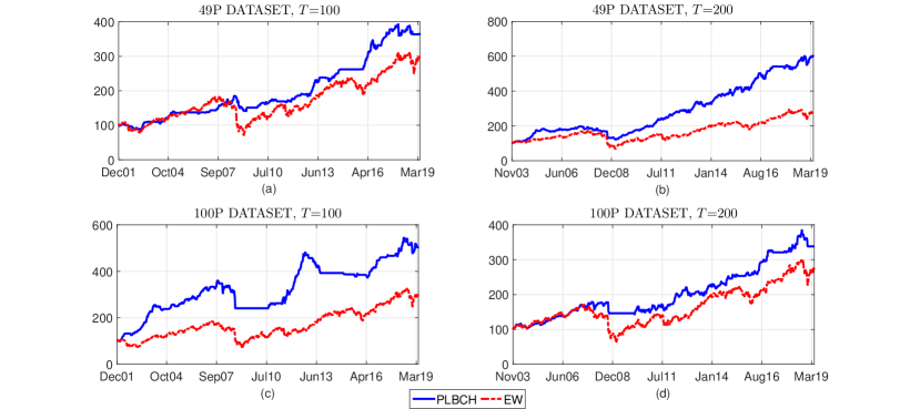
Figure 1: The figure displays the wealth provided by PLBCH and EW over time. Subfigures (a)—(b) display the results we obtain using the 49 Industry Portfolios (49P) dataset, implementing the rolling window procedure with, respectively, $T=100$ and $T=200$ observations. Subfigures (c)—(d) display the results we obtain using the 100 Portfolios Formed on Size and Book–to–Market (100P) dataset, implementing the rolling window procedure with, respectively, $T=100$ and $T=200$ observations.

Finally, we check that the post–penalization procedure turns out to be an effective tool to deal with the portfolio concentration issues highlighted by Bonaccolto et al. (2018). Indeed, it significantly mitigates the weight of the $s$–th asset; that is, the one whose return represents the response variable in the estimated quantile regression model. For instance, when using the 49P dataset with $T=100$, such a weight falls from an average value of 0.9310 with LBCH to an average value of 0.3621 with PLBCH.

5 Concluding remarks

We show that the performance of financial portfolios derived from penalized quantile regression models crucially depends on the specification of the penalty function, on the regularization parameter method selection and on the use of the post–penalization procedure. Although the properties of these methods have been widely studied in the statistical literature, they have never been tested from a financial viewpoint when building investment strategies using quantile regression models.

A joint analysis of six performance indicators providing information about risk, profitability and turnover highlights the significant improvements we can achieve going beyond the simple LASSO method. These improvements are clear when focusing on the risk dimension, in terms of a lower volatility and extreme risk. This is a relevant result in this study, as the expected shortfall represents the target measure we aim to minimize when estimating a quantile regression model. Surprisingly, we also record gains in terms of risk–adjusted return and profitability, outperforming the equally weighted portfolio, which is a benchmark known to be difficult to beat out–of–sample. In addition, our proposal turns out to be an effective tool to deal with the portfolio concentration issues highlighted by Bonaccolto et al. (2018), mitigating the weight of the stock whose return represents the response variable of the estimated regression models. Finally, the new strategies we propose in this study are computationally efficient, providing then an advantageous tool for several financial agents, such as traders and hedge funds, to improve the performance of their portfolios, while controlling the risk of incurring large losses during tail events.

Here, we build financial portfolios from quantile regression models estimated at the 5% level. It would be interesting to analyse how the results change when using other quantile levels, not only the ones belonging to the left tail of the return distributions (reflecting a pessimistic asset allocation), but also those which refer to the right tail (suitable when markets are trending upward). Furthermore, we can also combine the strategies resulting from different quantile levels in the range $(0,1)$, adapting them to the different market conditions, exploiting the strengths of the different asset allocation schemes over time. We include these further analyses in our research agenda.

References

- Acerbi and Tasche (2002) Acerbi, C. and D. Tasche (2002). Expected shortfall: A natural coherent alternative to value at risk. Economic Notes 31(2), 379–388.
- Artzner et al. (1999) Artzner, P., F. Delbaen, J. Eber, and D. Heath (1999). Coherent measures of risk. Mathematical Finance 9(3), 203–228.
- Assa (2015) Assa, H. (2015). Risk management under a prudential policy. Decisions in Economics and Finance 38(2), 217–230.
- Bassett et al. (2004) Bassett, G., R. Koenker, and G. Kordas (2004). Pessimistic portfolio allocation and choquet expected utility. Journal of Financial Econometrics 2(4), 477–492.
- Belloni and Chernozhukov (2011) Belloni, A. and V. Chernozhukov (2011). L1-penalized quantile regression in high-dimensional sparse models. The Annals of Statistics 39(1), 82–130.
- Bonaccolto et al. (2018) Bonaccolto, G., M. Caporin, and S. Paterlini (2018). Asset allocation strategies based on penalized quantile regression. Computational Management Science 15(1), 1–32.
- Bonaccolto and Paterlini (2019) Bonaccolto, G. and S. Paterlini (2019). Developing new portfolio strategies by aggregation. Annals of Operations Research (forthcoming).
- Brodie et al. (2009) Brodie, J., I. Daubechies, C. D. Mol, D. Giannone, and I. Loris (2009). Sparse and stable markowitz portfolios. PNAS 106(30), 12267–12272.
- Chen (2008) Chen, S. X. (2008). Nonparametric estimation of expected shortfall. Journal of Financial Econometrics 6(1), 87–107.
- Ciliberti et al. (2007) Ciliberti, S., I. Kondor, and M. Mézard (2007). On the feasibility of portfolio optimization under expected shortfall. Quantitative Finance 7(4), 389–396.
- DeMiguel et al. (2009) DeMiguel, V., L. Garlappi, F. J. Nogales, and R. Uppal (2009). A generalized approach to portfolio optimization: Improving performance by constraining portfolio norms. Management Science 55(5), 798–812.
- DeMiguel et al. (2009) DeMiguel, V., L. Garlappi, and R. Uppal (2009). Optimal versus naive diversification: How inefficient is the 1/N portfolio strategy? Review of Financial Studies 22, 1915–1953.
- Duchin and Levy (2009) Duchin, R. and H. Levy (2009). Markowitz versus the talmudic portfolio diversification strategies. Journal of Portfolio Management 35, 71–74.
- Fan and Li (2001) Fan, J. and R. Li (2001). Variable selection via nonconcave penalized likelihood and its oracle properties. Journal of the American Statistical Association 96(456), 1348–1360.
- Fan et al. (2012) Fan, J., J. Zhang, and K. Yu (2012). Vast portfolio selection with gross-exposure constraints. Journal of the American Statistical Association 107(498), 592–606.
- Fastrich et al. (2015) Fastrich, B., S. Paterlini, and P. Winker (2015). Constructing optimal sparse portfolios using regularization methods. Computational Management Science 12(3), 417–434.
- Gijbels and Herrmann (2018) Gijbels, I. and K. Herrmann (2018). Optimal expected-shortfall portfolio selection with copula-induced dependence. Applied Mathematical Finance 25(1), 66–106.
- Gilli and Këllezi (2002) Gilli, M. and E. Këllezi (2002). A global optimization heuristic for portfolio choice with VaR and Expected Shortfall. In E. J. Kontoghiorghes, B. Rustem, and S. Siokos (Eds.), Computational Methods in Decision-Making, Economics and Finance. Applied Optimization, Volume 74, pp. 167–183. Boston, MA: Springer.
- Giuzio (2017) Giuzio, M. (2017). Genetic algorithm versus classical methods in sparse index tracking. Decisions in Economics and Finance 40(1-2), 243–256.
- Giuzio and Paterlini (2018) Giuzio, M. and S. Paterlini (2018). Un–diversifying during crises: is it a good idea? Computational Management Science 16(3), 401–432.
- Hastie et al. (2009) Hastie, T., R. Tibshirani, and J. Friedman (2009). The Elements of Statistical Learning. Springer.
- Hautsch et al. (2014) Hautsch, N., J. Schaumburg, and M. Schienle (2014). Financial network systemic risk contributions. Review of Finance 19(2), 685–738.
- Koenker (2005) Koenker, R. (2005). Quantile regression. Number 38. Cambridge university press.
- Koenker and Bassett (1978) Koenker, R. and G. Bassett (1978). Regression quantiles. Econometrica 46(1), 33–50.
- Kratz et al. (2018) Kratz, M., Y. H. Lok, and A. J. McNeil (2018). Multinomial VaR backtests: a simple implicit approach to backtesting expected shortfall. Journal of Banking & Finance 88, 393–407.
- Kremer et al. (2018) Kremer, P. J., A. Talmaciu, and S. Paterlini (2018). Risk minimization in multi–factor portfolios: what is the best strategy? Annals of Operations Research 266(1-2), 255–291.
- Ledoit and Wolf (2008) Ledoit, O. and M. Wolf (2008). Robust performance hypothesis testing with the Sharpe ratio. Journal of Empirical Finance 15(5), 850–859.
- Lee et al. (2014) Lee, E. R., H. Noh, and B. U. Park (2014). Model selection via Bayesian information criterion for quantile regression models. Journal of the American Statistical Association 109(505), 216–229.
- Li and Zhu (2008) Li, Y. and J. Zhu (2008). L1-norm quantile regression. Journal of Computational and Graphical Statistics 17(1), 163–185.
- Markowitz (1952) Markowitz, H. (1952). Portfolio selection. The Journal of Finance 7, 77–91.
- Patton et al. (2019) Patton, A. J., J. F. Ziegel, and R. Chen (2019). Dynamic semiparametric models for expected shortfall (and Value–at–Risk). Journal of Econometrics 211(2), 388 – 413.
- Rockafellar and Uryasev (2000) Rockafellar, R. and S. Uryasev (2000). Optimization of conditional var. Journal of Risk 2(3), 21–41.
- Tibshirani (1996) Tibshirani, R. (1996). Regression analysis and selection via the lasso. Journal of the Royal Statistical Society, Series B 58(1), 267–288.
- Tu and Zhou (2011) Tu, J. and G. Zhou (2011). Markowitz meets Talmud: A combination of sophisticated and naive diversification strategies. Journal of Financial Economics 99(1), 204–215.
- Yamai and Yoshiba (2005) Yamai, Y. and T. Yoshiba (2005). Value–at–risk versus expected shortfall: a practical perspective. Journal of Banking & Finance 29(4), 997–1015.
- Yen and Yen (2014) Yen, Y. and T. Yen (2014). Solving norm constrained portfolio optimization via coordinate-wise descent algorithms. Computational Statistics and Data Analysis 76, 737–759.
- Zhang (2010) Zhang, C.-H. (2010). Nearly unbiased variable selection under minimax concave penalty. The Annals of Statistics 38(2), 894–942.