First-principles many-body non-additive polarization energies from monomer and dimer calculations only : A case study on water

Abstract

The many-body polarization energy is the major source of non-additivity in strongly polar systems such as water. This non-additivity is often considerable and must be included, if only in an average manner, to correctly describe the physical properties of the system. Models for the polarization energy are usually parameterized using experimental data, or theoretical estimates of the many-body effects. Here we show how many-body polarization models can be developed for water complexes using data for the monomer and dimer only using ideas recently developed in the field of intermolecular perturbation theory and state-of-the-art approaches for calculating distributed molecular properties based on the iterated stockholder atoms (ISA) algorithm. We show how these models can be calculated, and validate their accuracy in describing the many-body non-additive energies of a range of water clusters. We further investigate their sensitivity to the details of the polarization damping models used. We show how our very best polarization models yield many-body energies that agree with those computed with coupled-cluster methods, but at a fraction of the computational cost.

I Introduction

Ab initio intermolecular interaction models have come a long way in recent years. We have seen the development both of specific interaction models, for high-accuracy calculations on specific systems, and of classes of models designed to be more generally applicable to a broad range of systems. By and large, these models are constructed using well-defined theoretically motivated functional forms, with parameters either extracted from molecular properties, or fitted to a range of ab initio interaction energy calculations, or a combination of these. The successes of these approaches have now been well documented and include the fields of molecular organic crystal structure prediction, Welch et al. (2008); Cooper et al. (2008a); Price et al. (2010); Misquitta et al. (2008a) simulation of liquids such as water, Bukowski et al. (2007) high-accuracy spectroscopy (see for example Jankowski and Szalewicz (1998); Groenenboom et al. (2000); van der Avoird et al. (2010); Vissers et al. (2005)), and other bulk properties.

In principle, creating a model from first principles may seem reasonably straightforward: a functional form with a fixed number of parameters which are determined using as large a data set of ab initio interaction energies as is needed. This is of course a simplistic view of what is a complex fitting problem in a high dimensional space with parameters that are often heavily correlated. However, for the two-body interaction (here and elsewhere in this paper by ‘body’ we mean an interacting unit, that is, a molecule), particularly with the rigid-body approximation, this problem has been largely solved using advanced, hierachical fitting techniques in which the bulk of the parameters are extracted from the charge-density and static and frequency-dependent density linear-response functions or are given prior values (in the Bayesian sense) via a density-overlap model Misquitta and Stone (2016); Stone and Misquitta (2007); Misquitta et al. (2008a); Van Vleet et al. (2016); Van Vleet et al. (2018); Metz et al. (2016). Additionally, machine learning algorithms are being used, particularly for high-accuracy modelling of small systems Uteva et al. (2017), though these techniques are being used on larger systems too Li et al. (2017); Popelier (2015).

Many-body non-additive effects complicate matters considerably. Even with the rigid-body approximation, the dimension of the fitting space is much larger when many-body effects are included. Here, more than ever, we need recourse to physical models rather than brute-force fitting to computed data.

The importance of many-body effects cannot be disputed. The non-trivial consequences of many-body dispersion energies have been extensively documented in the recent literature in the condensed phase, or in low-dimensional systems, these effects can lead to qualitative deviations from the two-body additive description. Likewise, many-body polarization effects have been shown to play an important role in molecular organic crystals, Welch et al. (2008); Cooper et al. (2008b) interfaces, Harder et al. (2009); Misra and Blankschtein (2017) ion solvation, the anomalous properties of water, and more generally, in any system with strong permanent multipoles and high polarizabilities. Besides these there are many-body effects arising from the exchange energy, charge-delocalization energy (often termed “charge-transfer”, but see the discussion below), and the various couplings between these and the dispersion and polarization. In this paper we will be concerned with many-body polarization models only.

In some cases, it is possible to mimic the average effect of the many-body interactions by adjusting the parameters in the two-body model. For example, in bulk water the many-body polarization leads to a charge movement in the water molecules that can be used to approximate the effects of polarization without the need for an effective polarization model. This is of course only approximate and leads to models such as TIP4P that use a fixed enhanced dipole moment but are limited in applicability to situations where the water is ‘bulk-like’, and fail where the water molecules are in a manifestly different state, for example in clusters cis and at interfaces Harder et al. (2009); Misra and Blankschtein (2017). If we seek to develop models that are applicable to an ever wider range of applications, then we much describe these complex effects correctly, preferably from first principles.

In principle the development of a many-body polarization model is straightforward: the system is assigned permanent multipoles and static (zero-frequency) polarizabilities. These are coupled together and the polarization energy is determined through the self-consistent multipole-moment changes in a manner described by Stone Stone (2013). In some models Drude oscillators are used in place of point polarizabilities, but these do not differ in a fundamental way, except that we understand better how to increase the ranks of the point polarizabilities. The multipoles and polarizabilities need to be distributed for all but the smallest of molecules and they need to include terms of high enough rank to ensure convergence. The difficulty with the polarization model lies in the choice of damping: all polarization models need some form of damping to ensure that the many-body polarization energies are meaningful. While the choice of damping may not appear to have a significant effect on the two-body energies, the consequences for the many-body energies can be enormous, particularly as we increase the ranks of the polarizabilitity tensors.

Thus far there have been two main approaches to developing many-body models for water: the first approach combines a two-body (2B) interaction model with an $N$-body (NB) polarization model, and the second uses both a two-body and three-body (3B) model with non-additive contributions involving four and more bodies described using a polarization model. We will refer to these approaches as the “2B+NBpol” and “2B+3B+NBpol” models, respectively. Note that here and elsewhere in this paper we refer to a (water) molecule as a “body”. The advantage of the first approach is simplicity: such a model will be more efficiently evaluated in a simulation, but the latter approach is expected to be more accurate as it offers the possibility of including three-body non-additivity from the exchange and dispersion effects in addition to that from the induction contribution to the interaction energy. The disadvantage of the second approach is one of dimensionality: for rigid water molecules the 2B model is 6-dimensional, but the 3B model is 12-dimensional. If the water molecules are considered flexible then the number of dimensions increases to 12 and 21 respectively. This has meant that recent models based on the second approach, in particular the MB-pol model Babin et al. (2013, 2014), which includes molecular flexibility, and the CCpol23+ model, which does not, have been parameterised using an enormous amount of data. The three-body part of MB-pol used 12,000 water trimer calculations and CCpol23+ used more than 71,000 trimers. Additionally CCpol23+ used tetramers of water extracted from the known water hexamers.

Any model based on the 2B+NBpol approach will need far less data for its parameterization. However as this class of models relies entirely on the classical polarizable model for the many-body non-additivity, some, carefully chosen clusters of water are needed in practice to help tune the parameters in the polarization model so as to result in a reasonable description of the many-body effects. This is the approach taken by the DPP and DPP2 models. Kumar et al. (2010) Interestingly, the one exception to this is are the ASP-W potentials Millot et al. (1998) which are constructed without recourse to cluster data.

While extensive data sets of clusters of more than two molecules is a viable approach for the water molecule, for larger systems both the 2B+3B+NBpol and 2B+NBpol approaches can prove both computationally formidable and also cumbersome. As we seek to develop many-body interaction models for larger systems we need to find ways of reducing our dependence on data and also reduce fitting to a minimum. Indeed, with these considerations in mind, over the last few years we have developed techniques for constructing many-body polarization models from accurate distributed multipoles Misquitta et al. (2014) and distributed polarizabilities Misquitta and Stone (2018a), based both on a basis-space version Misquitta et al. (2014) of the iterated stockholder atoms (ISA) algorithm Lillestolen and Wheatley (2008) and a detailed understanding of the link between the polarization, charge-delocalization and induction energies made through Reg-SAPT(DFT) Misquitta (2013). While we have used some of these methods in developing the many-body model for the pyridine complex and have successfully used this model to find the two known forms as well as a new, third form of the pyridine crystal, Aina et al. (2017) we have never put these models to detailed tests of their capacity to describe the many-body energies of complexes. This is what we do now, using some of the extensive datasets available for the water system. Additionally, as we wish to explore the limits of this approach — that uses only monomer and dimer data — in the prediction of the many-body non-additive energies, we pose the following questions:

• Q1: Can many-body polarization models be developed from the properties of the monomer and dimer energy calculations only?

• Q2: Can we develop a systematic hierarchy of polarizability models of increasing rank, and how do the accuracies of these models vary with rank?

• Q3: How accurate are the damping models obtained from Reg-SAPT(DFT) and how sensitive are the many-body energies and cluster geometries to deviations from them?

The first question is central to this paper: we will show that under some assumptions, the many-body polarization energy can indeed be determined from monomer properties and dimer energies only; no more information is needed. The second question is posed as this question has never been addressed in a systematic study: most polarization models make use of dipole-dipole polarizabilities only, and only ASP-W4 Millot et al. (1998) and SCME Wikfeldt et al. (2013) make use of quadrupolar polarizabilities, but neither fare well on reproducing the energies of the water hexamers cis . As we shall show, the dipole-dipole polarizability model is a sweet spot for water, but for higher accuracy, particularly for systems with heavier atoms, higher ranking terms may be needed. Finally we pose the third question as we have previously argued that the true polarization energy (at second order) is well-defined through Reg-SAPT(DFT) Misquitta (2013) and this allows us to determine the polarization damping needed for a specified polarization model. Here we test just how close to optimum is this approach and what happens to the errors in the many-body energies if the damping parameters are altered from the proposed values.

II Computational details

The molecular properties used in this work were computed using the modified basis-space iterated stockholder atoms (BS-ISA) and the ISA-Pol algorithms implemented in CamCASP 6.0 Misquitta and Stone (2018b). The Kohn–Sham orbitals and orbital energies needed for these calculations were calculated using the DALTON2006 Helgaker et al. (2005) code with a patch from the SAPT Bukowski et al. (2008) code. We used the asymptotically corrected PBE0 Adamo and Barone (1999) functional with the d-aug-cc-pVTZ basis set. For the asymptotic correction we used the Fermi–Amaldi Fermi and Amaldi (1934) long-range form with the Tozer & Handy splicing Tozer and Handy (1998) and a shift computed using the vertical ionization energy of $0.4638$ Hartree Lias . The linear-response density functional calculations were performed using the hybrid ALDA+CHF kernel in CamCASP 6.0 Misquitta and Stone (2018b, 2016).

The SAPT(DFT) interaction energy calculations used to determine the induction energies and regularized induction energies for the polarization models were computed using CamCASP 6.0 Misquitta and Stone (2018b) with the above numerical details except that we used the aug-cc-pVTZ basis in the MC+BS format Williams et al. (1995) using a 3s2p1d1f mid-bond basis. Note that in CamCASP 6.0 the second-order exchange-induction energy is computed without the single-exchange ($S^{2}$) approximation using a closed-shell implementation of the general energy expression derived by Schaffer & Jansen Schäffer and Jansen (2012).

To develop the non-polarization terms in the two-body potential we used 2048 dimers selected at random using an algorithm based on Shoemake’s uniform random rotations scheme Shoemake (1992) which we have described in previous publications Stone and Misquitta (2007); Misquitta et al. (2008a); Misquitta and Stone (2016) and have implemented in the CamCASP program. SAPT(DFT) interaction energies were computed using the above basis but with CamCASP 5.9, that is, the $S^{2}$ approximation was used with $E^{(2)}_{\rm ind,exch}$. However as observed by Schaffer & Jansen, the error is largely cancelled with a corresponding error of the opposite sign in the $\delta^{\rm HF}_{\rm int}$ term.

III Notation & Nomenclature

In this paper we adopt the notation for the SAPT(DFT) interaction energy components introduced in a recent paper Misquitta and Stone (2016): $E^{(1)}_{\rm elst}$ and $E^{(1)}_{\rm exch}$ are the first-order electrostatic and exchange-repulsion energies, $E^{(2)}_{\rm IND}=E^{(2)}_{\rm ind,pol}+E^{(2)}_{\rm ind,exch}$ is the total second-order induction energy, $E^{(2)}_{\rm IND}({\rm Reg})=E^{(2)}_{\rm ind,pol}({\rm Reg})+E^{(2)}_{\rm ind,exch}({\rm Reg})$ is the total regularized second-order induction energy Misquitta (2013), $E^{(2)}_{\rm DISP}=E^{(2)}_{\rm disp,pol}+E^{(2)}_{\rm disp,exch}$ is the total dispersion energy, and $\delta^{\rm HF}_{\rm int}$ is the estimate of effects of third and higher order, primarily induction Jeziorska et al. (1987); Moszynski et al. (1996).

We will partition the total second-order induction energy, $E^{(2)}_{\rm IND}$, into a charge-delocalization (CD) and true polarization (POL) energy at second-order: $E_{\rm CD}^{(2)}$ and $E_{\rm POL}^{(2)}$. Higher-order terms will be defined below. Note that in previous works we have termed the charge-delocalization energy as the “charge-transfer” energy, which is the term used by much of the literature. Also note that what we will call the polarization energy is often, and confusingly, termed the “induction” energy in texts Stone (2013) and our past papers Misquitta and Stone (2008); Misquitta et al. (2008b).

Note that the SAPT energy components without exchange effects included are also termed “polarization” Jeziorski et al. (1994), but these are not the same as the polarization energies that arise from the conventional electromagnetic polarization that will be the focus of this paper.

IV The models: Derived Intermolecular Force-Fields (DIFF)

We have described the procedure used to develop the derived intermolecular force-fields, or DIFF models, in previous works Misquitta and Stone (2016). In brief, at long-range, distributed multipole expansions for the electrostatics, polarization and dispersion terms are computed from the unperturbed molecular properties, and at short-range the polarization and dispersion expansions are damped and electrostatic penetration, exchange-repulsion and charge-delocalization energies are described using an anisotropic Born–Mayer functional form, with the anisotropy described through atomic shape-functions. Here we list some of the important numerical choices made that are relevant to this work; the full potential specifications and parameters are provided in the Supplementary Information.

• Electrostatic multipoles were calculated using the ISA-A functional from the modified version Misquitta and Stone (2018a) of the basis-space iterated stockholder atoms (BS-ISA) algorithm Misquitta et al. (2014). Terms of maximum rank 4 were kept on all atoms, and the electrostatic expansion is not damped.

• Polarizability models were calculated using the ISA-Pol algorithm Misquitta and Stone (2018a) in a manner consistent with the electrostatic moments. The non-local polarizabilites from the ISA-Pol algorithm include terms from ranks 0 to 4 and are cumbersome to be used directly, consequently we have localized the polarizabilities Misquitta and Stone (2018a) to result in three models of maximum ranks 1, 2 and 3. These polarizability models are local but anisotropic and include all intramolecular couplings. The polarization damping models are described below in detail.

• Dispersion models for the water dimer are identical to those reported in an earlier work Misquitta and Stone (2018a). They were calculated in a similar manner from the frequency-dependent localized and isotropic ISA-Pol polarizabilities, with all site pairs including terms from $C_{6}$ to $C_{12}$. We have used the Tang & Toennies damping functions Tang and Toennies (1992) with damping parameters determined using the scaled-ISA-exponents algorithm Misquitta and Stone (2018a) which gives damping parameters: $\beta_{\rm disp}^{\mathrm{OO}}=1.7794$, $\beta_{\rm disp}^{\mathrm{OH}}=1.9011$, and $\beta_{\rm disp}^{\mathrm{HH}}=2.0227$ atomic units.

• Short-range terms were modelled using an anisotropic Born–Mayer functional form in site–site form Misquitta and Stone (2016). The parameters in this part of the model were determined by fitting to reference SAPT(DFT) interaction energies which fully account for the electrostatic penetration, exchange-repulsion and charge-delocalization energies.

The full specifications of the model parameters are included in the supporting information.

Note that in previous works we have fitted the short-range interaction model in a multi-step procedure that used the distributed density-overlap model as a means to obtain prior values to the model parameters Misquitta and Stone (2016). We have not done this here as the water molecule is small enough that all parameters are well determined by the computed data.

IV.1 The polarization models

The damped classical polarization model is described comprehensively in texts such as that by Stone Stone (2013) so we outline only the points that relate to this paper. The classical polarization energy of a molecule $A$ in a cluster is defined as:

$$E_{\rm pol,cl}{}(A) =\frac{1}{2}\sum_{a\in A}\sum_{B\neq A}\sum_{b\in B}\sum_{tu}\Delta Q^{a}_{t}f_{n(tu)}(\beta_{\rm pol}^{ab}R_{ab})T^{ab}_{tu}Q^{b}_{u},$$ (1)

where the ranks of the moments are given in the compact form $t\equiv l\kappa$ where $l=0,1,2,\dots$ is the angular momentum quantum number and $\kappa=0,1c,1s,\dots,lc,ls$ labels the real components of the spherical harmonics of rank $l$ (see Appendix B in Stone Stone (2013)). $Q^{a}_{t}$ is the multipole moment operator for moment $t$ at site $a$, and $T^{ab}_{tu}$ is the interaction tensor Stone (2013) which describes the interaction between a multipole $Q^{b}_{u}$ at site $b$ and a multipole $Q^{a}_{t}$ at site $a$. $f_{n(tu)}(\beta_{\rm pol}^{ab}R_{ab})$ is a damping function of order $n$. Here $n$ is a function of the tensor ranks $t$ and $u$, and if $t=l_{1}\kappa_{1}$ and $u=l_{2}\kappa_{2}$, then $n=l_{1}+l_{2}+1$. We assume that the damping depends only on the distance $R_{ab}$ between sites $a$ and $b$ and not on their relative orientation. This is an approximation that needs assessment, but we do not address this issue in this paper. The strength of the damping is governed by the damping parameter $\beta_{\rm pol}^{ab}$. In the above expression, $\Delta Q^{a}_{t}$ is the change in multipole moment $t$ at $a$ due to the self-consistent polarization of site $a$ in the field of all sites on other molecules, and is given by

$$\Delta Q^{a}_{t} =-\sum_{a^{\prime}\in A}\sum_{B\neq A}\sum_{b\in B}\sum_{t^{\prime}v}\alpha^{aa^{\prime}}_{tt^{\prime}}f_{n(t^{\prime}v)}(\beta_{\rm pol}^{a^{\prime}b}R_{a^{\prime}b})T^{a^{\prime}b}_{t^{\prime}v}(Q^{b}_{v}+\Delta Q^{b}_{v}),$$ (2)

where $\alpha^{aa^{\prime}}_{tt^{\prime}}$ is the distributed polarizability for sites $(a,a^{\prime})$ which describes the response of the multipole moment component $Q^{a}_{t}$ at site $a$ to the $t^{\prime}$-component of the field at site $a^{\prime}$. To find $\Delta Q^{a}_{t}$ we need to solve eq. (2) iteratively and this leads to the significant computational cost of the classical polarization model, though there are now methods to reduce this cost Albaugh and Head-Gordon (2017); Lagardère et al. (2017). If $\Delta Q^{b}_{v}$ is dropped from the right-hand-side of this equation then the resulting $\Delta Q^{a}_{t}$, when inserted in eq. (1) leads to the second-order polarization energy, $E^{(2)}_{\rm pol,cl}$.

In the polarization models used in this paper we assume the Tang–Toennies form for the damping functions Tang and Toennies (1984). Further we use the localized form Misquitta and Stone (2008); Misquitta et al. (2008b) of the distributed polarizability tensor, that is, the non-local polarizability $\alpha^{aa^{\prime}}_{tu}$ in eq. (2) is replaced by $\alpha^{a}_{tu}\delta_{aa^{\prime}}$, where $\delta_{aa^{\prime}}$ is the Kronecker-delta and $\alpha^{a}_{tu}$ is the localized polarizability tensor of the same rank.

Without the damping functions, the classical polarization model can be used to determine the polarization energy at long-range only, where orbital overlap effects are negligible. At short-range, damping needs to be included to suppress the $1/R$ divergences that set in as $R\rightarrow 0$. Besides the elimination of the mathematical singularity, the damping functions are also required to enable the damped classical polarization energies to match the reference, non-expanded polarization energies. This poses a problem as neither SAPT(DFT) nor SAPT have an explicit polarization energy term, instead in both theories the induction energy can be considered the sum of the polarization (POL) and charge-delocalization (CD) energies Misquitta (2013). To complicate matters, just about any partitioning of the induction energy into CD and POL is consistent with a particular damped classical polarization model as long as the CD component is exponentially decaying (and thereby lacks a multipole expansion). That is, there are infinitely many damped classical polarization models that are consistent with the SAPT(DFT) induction energies. This would not be a problem if we were interested in dimer energies alone, but, as was already indicated by Misquitta Misquitta (2013), and as we demonstrate here with extensive datasets, the choice of damping can lead to vastly different predictions for the many-body polarization energies, and the system geometries. Consequently the choice of charge-delocalization energy is crucial.

IV.1.1 The charge-delocalization (CD) energy

The charge-delocalization may be thought of as a quantum delocalization process in which there is a (typically small) probability of the electronic charge density of a molecule to tunnel onto the atomic sites of a neighbouring molecule Misquitta (2013). The energy of stabilization of this process is the charge-delocalization energy. The physical origin of the CD energy is distinct from that of the classical polarization energy which originates from local responses in the charge denstiy. In fact, no polarization model with only rank 1 (dipole-dipole) polarizabilities and those of higher ranks can describe the CD process. Instead the charge movement in the CD process probably needs to be described by the rank 0 by 0 polarizabilities, also called charge-flow polarizabilities (see Chapter 9 in Stone Stone (2013)). These are non-local and are thus able to describe charge movement across a system Misquitta and Stone (2006); Misquitta et al. (2010); Liu et al. (2011) but are rarely applied in polarization models. While the non-local polarizabilities, including the charge-flow terms, are computed as part of the ISA-Pol calculation Misquitta and Stone (2018a), they are subsequently transformed away into higher-ranking polarizabilities using localization algorithms Le Sueur and Stone (1994); Lillestolen and Wheatley (2007). Even if these terms were retained, it is not clear how to use them directly in calculations of the CD energy. Consequently when developing classical polarization models with the localized polarizability models such as those we will use here, we need to ensure that the models are constructed to model only that part of the induction energy associated with local responses. That is, the charge-delocalization energy, which involves longer ranged charge movement, must be separated out from the induction.

Regularized SAPT(DFT) in brief: We use the definition of the CD energy based on regularised SAPT(DFT) Misquitta (2013), or Reg-SAPT(DFT). In this approach, the second-order induction energy is split into (second-order) polarization and (second-order) charge-delocalization contributions using a modified electron-nuclear interaction operator. Conceptually this involves interpreting the charge-delocalization energy as arising from a tunneling of the charge of one monomer into the attractive potential well arising from an electron-deficient site in a partner monomer. More specifically, we begin with the second-order induction energy of a molecule (A): this is the energy of stabilization in response to the total electrostatic potential arising from the unperturbed partner (B). In Reg-SAPT(DFT) we write the regularized electrostatic potential of monomer B as $\omega^{\rm B}_{\rm Reg}$ given by:

$$\omega^{\rm B}_{\rm Reg}({\mathbf{r}}) =-\sum_{\beta\in\mathrm{B}}Z_{\beta}\frac{1}{|{\mathbf{r}}-{\mathbf{R}}_{\beta}|}\left(1-e^{-\eta|{\mathbf{r}}-{\mathbf{R}}_{\beta}|^{2}}\right)+\int\frac{\rho^{\rm B}({\mathbf{r}^{\prime}})}{|{\mathbf{r}}-{\mathbf{r}^{\prime}}|}d{\mathbf{r}^{\prime}},$$ (3)

where $\beta$ labels the nuclei of monomer B, $Z_{\beta}$ is the nuclear charge located at position ${\mathbf{R}}_{\beta}$, $\rho^{\rm B}({\mathbf{r}})$ is the unperturbed electronic density of B, and $\eta$ is the regularization parameter. The regularized second-order “polarization” (not to be confused with the classical polarization energy) component of the induction energy is then defined as:

$$E^{(2)}_{\rm ind,pol}({\rm Reg})\mathrm{[A]} ={\sum_{r\neq 0}}\frac{|<\Phi^{\mathrm{A}}_{r}|\hat{\Omega}^{\rm B}_{\rm Reg}|\Phi^{\mathrm{A}}_{0}>|^{2}}{E^{\mathrm{A}}_{0}-E^{\mathrm{A}}_{r}},$$ (4)

where $\hat{\Omega}^{\rm B}_{\rm Reg}=\sum_{i}\omega^{\rm B}_{\rm Reg}({\mathbf{r}}_{i})$ is the many-body form of the electrostatic potential of monomer B, and $\Phi^{\mathrm{A}}_{r}$ and $E^{\mathrm{A}}_{r}$ are the excited states and energies of monomer A. A similar expression applies for $E^{(2)}_{\rm ind,pol}({\rm Reg})\mathrm{[B]}$. $E^{(2)}_{\rm ind,pol}({\rm Reg})$ is then the sum of the contributions from monomers A and B. This expression is readily evaluated using linear-response theory within the SAPT(DFT) framework, as is the accompanying second-order regularized exchange-induction contribution Misquitta (2013) without the single-exchange approximation Schäffer and Jansen (2012). These techniques are available in the CamCASP 6.0 code and have also been recently implemented in the Molpro code Hesselmann (2019).

The extent of the regularization is controlled by $\eta$: as $\eta\rightarrow\infty$ the regularization is switched off and we recover $E^{(2)}_{\rm IND}$. For any finite and positive value of $\eta$ we suppress some fraction of the second-order induction energy, and with $\eta=3.0$ a.u., Misquitta has demonstrated that is possible to suppress the CD contribution to $E^{(2)}_{\rm IND}$ thereby allowing us to define the second-order polarization energy as

$$E_{\rm POL}^{(2)} =E^{(2)}_{\rm IND}({\rm Reg})\equiv E^{(2)}_{\rm ind,pol}({\rm Reg})+E^{(2)}_{\rm ind,exch}({\rm Reg}).$$ (5)

And the second-order charge-delocalization energy is defined as the difference:

$$E_{\rm CD}^{(2)} =E^{(2)}_{\rm IND}-E^{(2)}_{\rm IND}({\rm Reg})$$ (6)

$$\equiv\left(E^{(2)}_{\rm ind,pol}-E^{(2)}_{\rm ind,pol}({\rm Reg})\right)+\left(E^{(2)}_{\rm ind,exch}-E^{(2)}_{\rm ind,exch}({\rm Reg})\right).$$ (7)

Notice that both $E_{\rm POL}^{(2)}$ and $E_{\rm CD}^{(2)}$ contain contributions from the exchange-induction energy. This fundamentally differentiates $E_{\rm POL}^{(2)}$ from the second-order induction “polarization” energy, $E^{(2)}_{\rm ind,pol}$, defined in SAPT(DFT).

The strength of this approach is that both $E_{\rm POL}^{(2)}$ and $E_{\rm CD}^{(2)}$ are well-defined in the complete basis set limit and $E_{\rm CD}^{(2)}$ is exponentially decaying as would be expected on physical grounds, even for very strongly bound complexes Misquitta (2013). However the downsides of this approach are that there is as yet no rigorous way of determining which value of $\eta$ exactly suppresses the charge-delocalization states in all cases, and in its present implementation the technique is applicable at second-order only. As has been demonstrated by Misquitta & Stone Misquitta and Stone (2016), the second difficulty can be overcome using the classical polarization model. We describe how this is done in  §IV.1.4 below. The first issue is the more challenging one as, while Misquitta has argued Misquitta (2013) that $\eta=3.0$ a.u. is an appropriate value for the regularization parameter, a more general algorithm to determine $\eta$ is needed.

Fitting the polarization model damping to $E_{\rm POL}^{(2)}$: Once we have determined the $E_{\rm POL}^{(2)}$ energies for a representative set of dimers, the polarization model damping in eq. (1) and eq. (2) can be determined by fitting to these energies. Since $E_{\rm POL}^{(2)}$ is equivalent to the classical polarization energy evaluated at the first step of the self-consistent process, no iterations are performed when determining the damping. That is, at this stage, the polarization energy is computed in response to the permanent fields only.

It may seem paradoxical that the many-body polarization energies can depend strongly on the definition of the charge-delocalization energy; after all the former arises from long-range interactions while the latter is a short-range phenomenon. The key issue here is that the polarization model damping (a short-range effect) depends on the definition of the CD energy, and so the induced moments also depend on the CD energy. These induced moments then interact with other bodies in the system through the long-range electrostatic interaction, and thereby can have major consequences for the energy of clusters or the condensed phase.

IV.1.2 Polarization in the DIFF models for water

We have created three DIFF polarization models for water with maximum polarizability ranks 1, 2 and 3, respectively. As already stated, the distributed polarizability models were computed using the ISA-Pol algorithm Misquitta and Stone (2018a) and these include anisotropy, and consequently also include couplings between the ranks. These localized models are fully coupled in the sense that polarization effects within the water molecule are fully accounted for. However, like the ISA-DMA multipoles, they have been computed for a fixed water geometry and will therefore be incorrect when applied to water molecules in different conformations. We note here that in previous works we have often limited the polarizability ranks Misquitta and Stone (2008); Misquitta et al. (2008b) on the hydrogen atoms to rank 1 (dipole-dipole), but here we have used the same maximum rank on all atoms.

There are three unique site-pairs in the water dimer (O…O, O…H, and H…H) and we associate each of these with a unique damping parameter, consequently we need to select dimers with suitable close contacts so as to be able to extract the damping information from the $E_{\rm POL}^{(2)}$ energies. Following earlier work Misquitta (2013) we use the three dimer orientations shown in Figure 1, and for each dimer orientation, $E^{(2)}_{\rm IND}({\rm Reg})$ energies are computed at several intermolecular separations. The polarization damping parameters, $\beta_{\rm pol}^{\mathrm{OO}}$, $\beta_{\rm pol}^{\mathrm{OH}}$, and $\beta_{\rm pol}^{\mathrm{HH}}$ for the three DIFF models are shown in Table 1, and in Figure 2 we display the scatter plot of $E^{(2)}_{\rm IND}({\rm Reg})$ energies versus the corresponding energies from the three DIFF polarization models. We see that the O…O pair needs more damping (a smaller damping coefficient) than the H…H pair, with the mixed, O…H damping coefficient intermediate. Further, as the maximum rank of the polarizability terms decreases, $\beta_{\rm pol}^{\mathrm{OH}}$ increases, presumably to make up for the missing effects. The polarization energies are most sensitive to the O…H cross term and least sensitive to the H…H term. In fact, with the data available to us, we were unable to precisely determine the H…H polarization damping parameter other than to state that it is large and close to the chosen value of $\beta_{\rm pol}^{\mathrm{HH}}=2.0$ a.u. To determine the damping for the O…O site pair we needed to compromise by focusing only on dimers with interaction energy less than $45.0$ $\,\rm{kJ\,mol}^{-1}$, or just over twice the absolute binding energy of the water dimer. It was not possible to find a damping model that worked for the more repulsive configurations, presumably because the anisotropy of the oxygen atom in water requires an angular dependence in the $\beta_{\rm pol}^{\mathrm{OO}}$ parameter.

These damping models combined with the polarizabilities and the appropriate two-body models result in the DIFF-L$n$pol models, where $n=1,2,3$ indicates the maximum rank of the polarizability tensors included in the model.

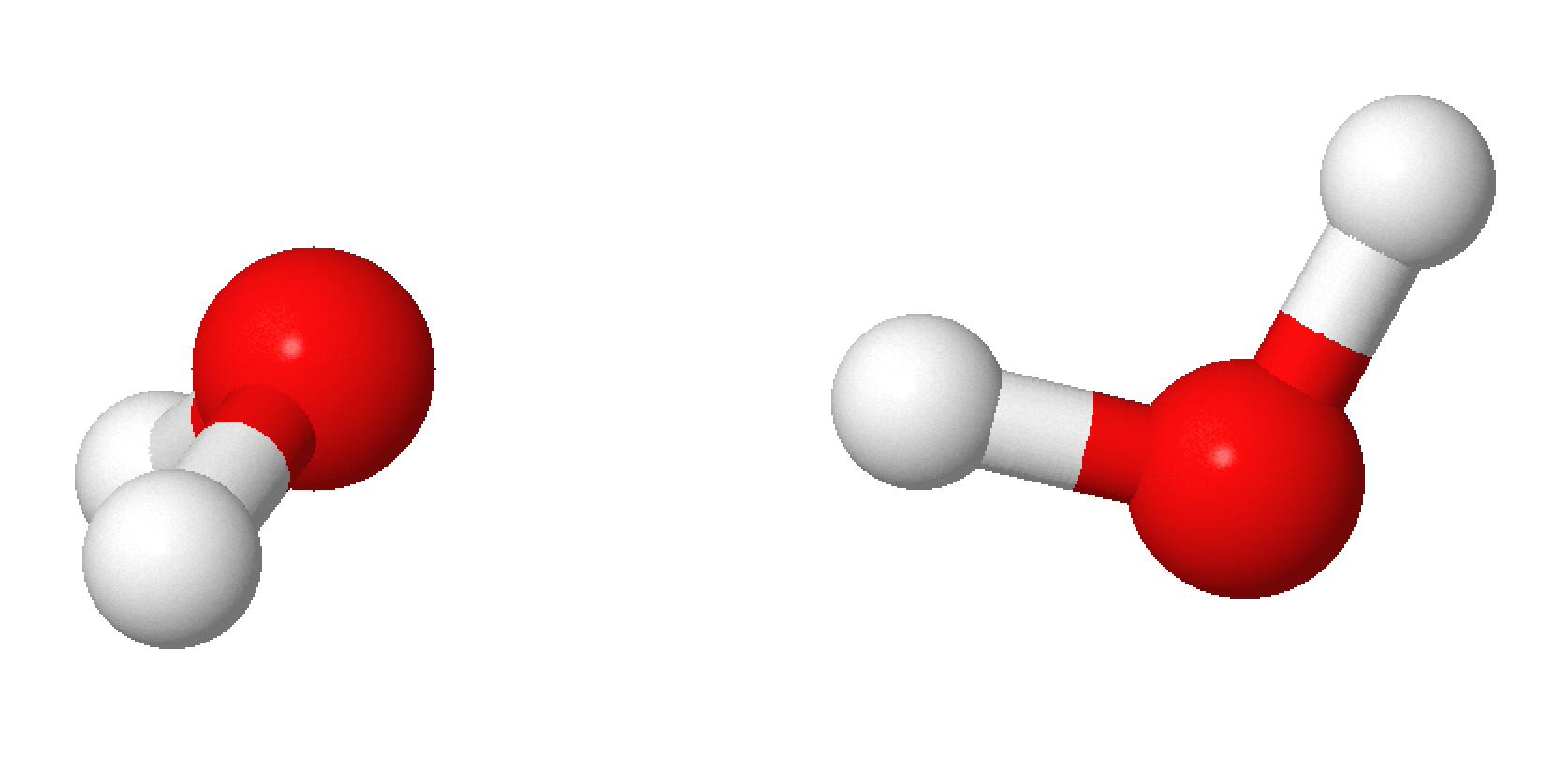
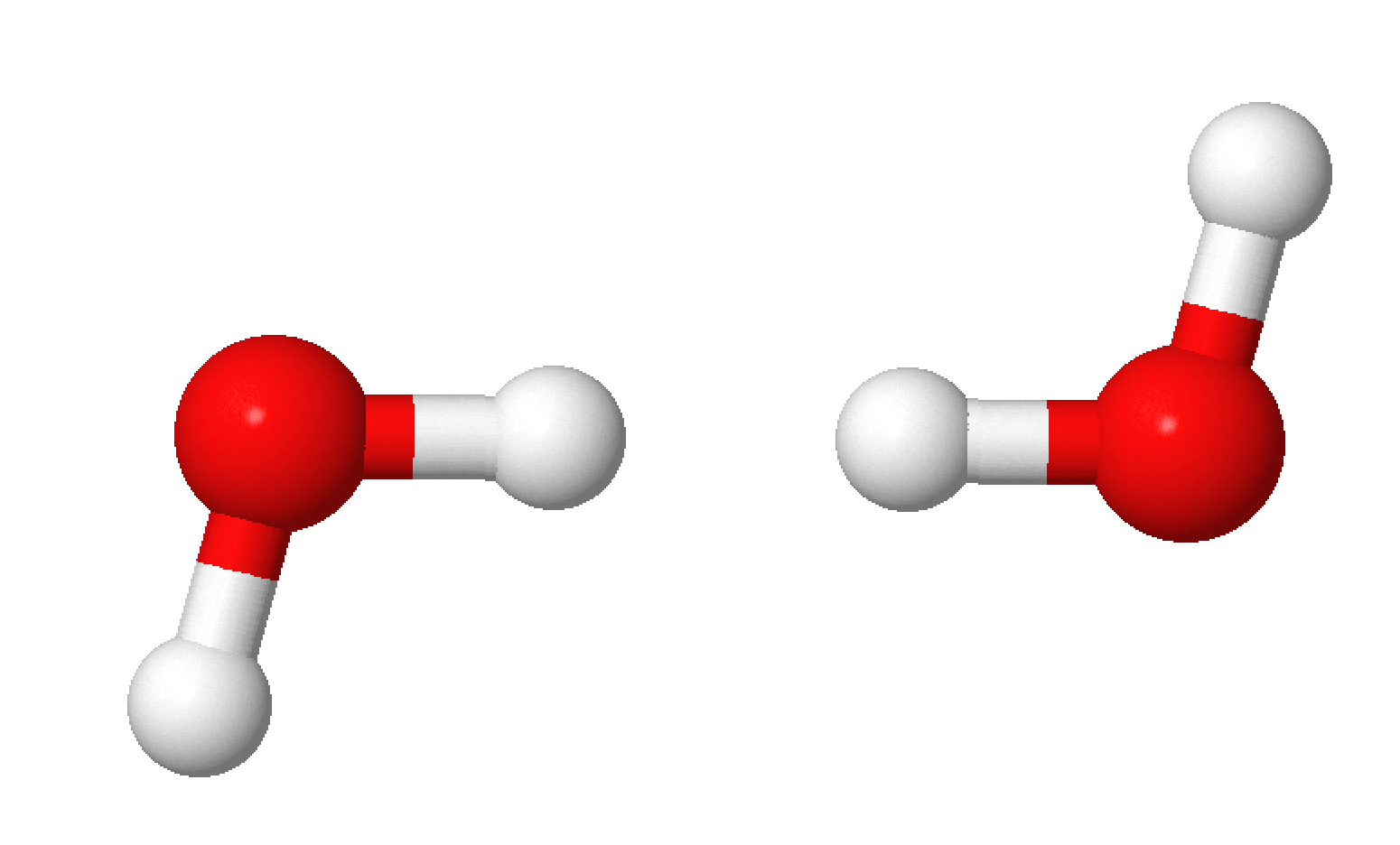
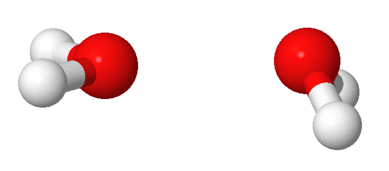
[-5pt](a) O..H contact [-5pt](b) H..H contact [-5pt](c) O..O contact

Figure 1: A representative sample of the water dimer configurations used in determining the polarization model damping parameters. In case (c) the angles of the planes of the two water molecules were sampled in 30° intervals. In all cases the dimer separations were sampled along the O..O separation vector.

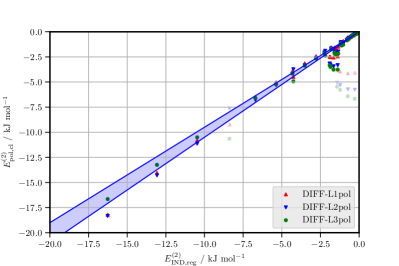
Figure 2: Scatter plot of second-order polarization energies computed using the three DIFF models against the reference $E^{(2)}_{\rm IND}({\rm Reg})$ energies computed for the dimer orientations shown in fig. 1. The solid points denote dimers with total energy less than $45.0$ $\,\rm{kJ\,mol}^{-1}$ and the faded points denote dimers with larger total interaction energies. The latter were not considered when determining the damping parameters for this model.

	IP		DIFF
	$x=0$	$x=0.5$	$x=1$	$x=1.5$
L3:
$\beta_{OO}$	1.926	1.588	1.25	0.912
$\beta_{OH}$	1.926	1.698	1.47	1.242
$\beta_{HH}$	1.926	1.963	2.00	2.037
L2:
$\beta_{OO}$	–	–	1.25	–
$\beta_{OH}$	–	–	1.57	–
$\beta_{HH}$	–	–	2.00	–
L1:
$\beta_{OO}$	1.926	1.588	1.25	0.912
$\beta_{OH}$	1.926	1.803	1.68	1.557
$\beta_{HH}$	1.926	1.963	2.00	2.037

Table 1: Polarisation damping parameters used for each model used in this work. The column titled “IP” indicates the damping based on the ionization potential of water (see text for details), and “DIFF” indicates the optimized damping for the DIFF models.

IV.1.3 Alternative polarization damping models

In addition to the DIFF-L$n$pol models described above we have explored models with alternative polarization damping in order to shed light on the importance of the choice of damping on the many-body energies and energy landscape.

In an early work on what were then termed “induction models”, Misquitta, Stone & Price recommended that the induction damping be determined from the molecular ionization potentials according to the formula Misquitta et al. (2008b):

$$\beta_{\rm pol}^{\mathrm{IP}}=\sqrt{2I_{A}}+\sqrt{2I_{B}},$$ (8)

where $I_{A/B}$ (in a.u.) are the vertical ionization potentials for monomers A and B. Notice that unlike the three-parameter DIFF damping models, this procedure results in a single parameter for all site pairs: that is, the damping depends on the interacting molecules as a whole. Despite this simplicity this damping model, which we will call the IP-based model, was shown to work remarkably well for a set of systems, but with this model the damped polarization energy was always close to $E^{(2)}_{\rm IND}$; that is, the total second-order induction energy which includes both the polarization and charge-delocalization energies at second-order.

In Figure 3 we display $E^{(2)}_{\rm IND}$ and $E^{(2)}_{\rm IND}({\rm Reg})$ for the water dimer in the hydrogen-bonded configuration. Also displayed are polarization models all with maximum rank of 3 but with different damping models. First of all, the DIFF-L3pol model can be clearly seen to reproduce $E^{(2)}_{\rm IND}({\rm Reg})$, but as found by Misquitta et al. Misquitta et al. (2008b), the IP-damped model reproduces $E^{(2)}_{\rm IND}$. We also display two additional models, one over-damped and the other under-damped, but intermediate to the DIFF-L3pol model and the IP-based one. The damping coefficients used in these four polarization models are related through linear interpolation with the parameter $x$ determining the model as follows:

$$\beta_{\rm pol}^{ab}(x)=\beta_{\rm pol}^{\mathrm{IP}}+x(\beta_{\rm pol}^{ab}-\beta_{\rm pol}^{\mathrm{IP}}),$$ (9)

where $\beta_{\rm pol}^{\mathrm{IP}}=1.926$ a.u. is the IP-based damping derived using eq. (8) using a vertical ionization of $0.4638$ a.u. Lias , and $\beta_{\rm pol}^{ab}$ are the optimized DIFF damping parameters for site-pair $ab$ shown in Table 1. Varying $x$ allows us to smoothly interpolate between the significantly underdamped IP-based damping model ($x=0.0$), through a moderately underdamped $x=0.5$ model, to the optimized DIFF model ($x=1.0$), and to an overdamped model with $x=1.5$. We have created complete interaction models for $x=0.0,0.5,1.0,~{}\text{and}~{}1.5$ for the polarization models with maximum rank 1 and 3, and can therefore perform energy evaluations and geometry optimizations with these models. The second-order polarization energies from the $x=0.5$ and $x=1.5$ models are displayed in Figure 3.

The range of polarization models available to us (both in rank and in choice of damping model) will allow us to evaluate the performance of these models in ways not possible before. In particular, we will be able to assess the predictive power of the DIFF damping models based on $E^{(2)}_{\rm IND}({\rm Reg})$ energies as described earlier in this section, and the availability of entire interaction models with different polarization damping will allow us to assess the importance of the choice of damping on the structures of water clusters.

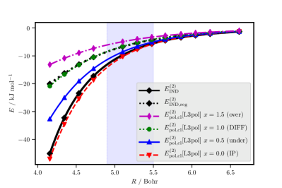
Figure 3: The second-order induction energy, $E^{(2)}_{\rm IND}$, regularised induction, $E^{(2)}_{\rm IND}({\rm Reg})$, and second-order polarization energies from the ISA-Pol-L3 polarizabilities with various damping models, all plotted as a function of the O..O separation in the water dimer in its hydrogen-bonded configuration (dimer (a) in fig. 1). As explained in the text, $x=1.5$ is the over-damped model, $x=1.0$ is the DIFF model with damping obtained from the regularised induction energies, $x=0.5$ is an underdamped model, and $x=0.0$ is an even more underdamped model derived from the ionisation energies of the water molecules.

IV.1.4 The infinite-order polarization charge-delocalization

Before moving on we note that having obtained the DIFF damping parameters, we can proceed to define the infinite-order CD and POL energies. Following Misquitta & Stone Misquitta and Stone (2016), this is done by first approximating the infinite-order induction energy as:

$$E^{(2-\infty)}_{\rm IND}\approx E^{(2)}_{\rm IND}+\delta^{\rm HF}_{\rm int}$$ (10)

and then defining the two-body infinite-order charge-delocalization energy to be

$$E_{\rm CD}^{(2-\infty)} =E^{(2-\infty)}_{\rm IND}-E_{\rm POL}^{(2-\infty)}$$

$$\approx E^{(2)}_{\rm IND}+\delta^{\rm HF}_{\rm int}-E^{(2-\infty)}_{\rm pol,cl},$$ (11)

where $E_{\rm POL}^{(2-\infty)}$ is the infinite-order polarization energy which is approximated by $E^{(2-\infty)}_{\rm pol,cl}$ from the classical polarization model iterated to convergence (see eq. (1) and eq. (2)). While this expression is readily implemented, it has a drawback in that the definition depends on the type of polarization model used, but this dependence is relatively minor.

The CD contributions from higher than second order are important and actually dominate at the H-bonded minimum energy dimer geometry: Here $E_{\rm CD}^{(2)}=-0.95$ $\,\rm{kJ\,mol}^{-1}$, but using $E^{(2-\infty)}_{\rm pol,cl}$ from the DIFF-L3pol polarization model we get, from eq. (11), $E_{\rm CD}^{(2-\infty)}=-3.30$ $\,\rm{kJ\,mol}^{-1}$, which is in good agreement with the ALMO(CCSD) result of $-3.51$ $\,\rm{kJ\,mol}^{-1}$ from Azar & Head-Gordon Azar and Head-Gordon (2012).

IV.1.5 Summary of main features of the DIFF polarization models

• Only 1-body and 2-body information is used. To construct the polarization models we need the molecular multipole moments and the molecular static polarizabilities. Both are 1-body properties that depend on many-body effects only through the dependence of the molecular conformation on the many-body interactions. The damping is determined using only two-body second-order induction energies calculated through Reg-SAPT(DFT).

• Reg-SAPT(DFT) allows us to define a definite damping model whose parameters vary only with the ranks of the multipole and polarizability models.

• Models of arbitrary rank can be created. The algorithm present here can be used to develop models of any rank or complexity. That is, while we will use multipole models with maximum rank 4 and anisotropic, fully coupled point-polarizability models with maximum ranks 1, 2 and 3, it should be equally possible to use Drude oscillator models with multipoles represented by point charges only.

It is perhaps the first of these points which is the most important: In the above procedure, no many-body information is used. In this respect, the models we present in this paper will differ from almost every other previously developed many-body polarization model.

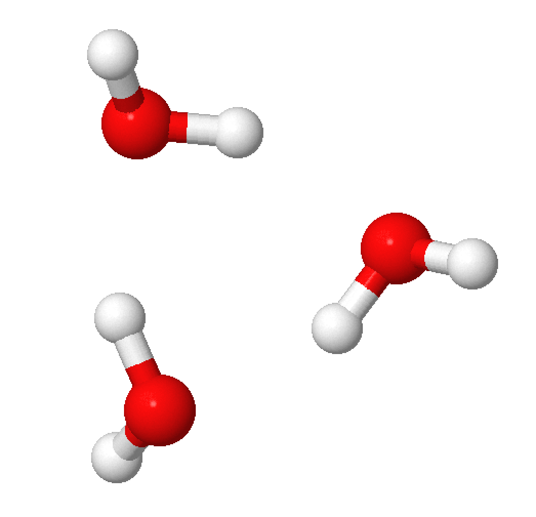
Figure 4: Water trimer structure.

V Assessment of the DIFF models

Ideally we would use the DIFF models to simulate various bulk properties of water, but this is not yet possible as even the simplest of these models cannot yet be used in mainstream simulation programs. While this may be possible soon, at present we are limited to tests on water clusters only. In some ways, this is advantageous as one of the main aims of this paper is to assess the predictive power of the DIFF models for the many-body energies, and a detailed analysis of water clusters of various sizes can allow us to make this assessment in an unambiguous manner as we have very accurate energies and optimized geometries for a whole range of water clusters from high-accuracy theory, as well as some information from experiment.

V.1 Trimers: Three-body (3B) non-additivity

The water trimers provide us with the first test of the capability of the DIFF models to describe the non-additive energies. We first use the reference trimer set from Liu et al. Liu et al. (2017) which consists of variations of the water trimer in its minimum energy configuration shown in Figure 4 with O…O bonds changed in a systematic manner. The trimer non-additive energies have been computed by Liu et al. using second-order Møller–Plesset (MP2) perturbation theory at the complete basis-set (CBS) limit. Note that the monomer geometries used for these trimers is the same as that used to construct the DIFF models and consequently the DIFF multipoles and polarizabilities are appropriate for these trimers.

In Figure 5 we display the non-additive 3B energies for these trimers from the DIFF models as well as from the AMOEBA model studied by Liu et al. Liu et al. (2017) The performance of all models is good with energy differences not exceeding 2 $\,\rm{kJ\,mol}^{-1}$, but the DIFF-L2pol and DIFF-L3pol models show the best agreement with the MP2/CBS data with most of the differences being substantially less than 0.5 $\,\rm{kJ\,mol}^{-1}$. The DIFF-L1pol model tends to underestimate the 3B non-additive energies, but usually this by less than 1 $\,\rm{kJ\,mol}^{-1}$, and for the lowest energy trimers (structures 0 and 1) this model comes closer to MP2 reference energies than the others.

In Figure 6 we display the 3B non-additive energies from the L1 and L3 polarization models with the alternative damping models described in  §IV.1.3. The models with maximum rank 1 (L1pol), that is, those that include dipole-dipole polarizabilies only are not very sensitive to the choice of damping. The 3B energies for these models vary by just over 5 $\,\rm{kJ\,mol}^{-1}$ in the worse case, but by around 2 $\,\rm{kJ\,mol}^{-1}$ for the majority of the 24 trimers. This shows that, at least for the trimers, the dipole-dipole polarization models are not too sensitive to the choice of damping model.

On the other hand, also shown in Figure 6 is the sensitivity of the polarization models with maximum rank 3 (L3pol) to the choice of damping, and here we see a very different picture. The DIFF-L3pol model with its damping determined by fitting to the $E^{(2)}_{\rm IND}({\rm Reg})$ energies is the best, with a near perfect agreement with the MP2/CBS reference energies. All the other damping models result in vastly different 3B non-additive energies. The IP-based damping model ($x=0.0$), which reproduces $E^{(2)}_{\rm IND}$ for the dimers (see Figure 3), results in an overestimation of the 3B non-additivity by more than a 100%, and for the $x=0.5$ model the overestimation is over 30%. At the other end, the over-damped $x=1.5$ model underestimates the non-additivity by more than 30%.

In Figure 7 we display the mean-absolute errors (MAEs) of the three polarization models as a function of the interpolation parameter $x$ (see eq. (9)). We see that for the L1 polarization model the MAE shows a shallow minimum at $x=0.4$, that is, for this model and for the timers used in this test, the dipole-dipole polarization model needs to be under-damped. However, for the L2 and L3 polarization models there is a very clear and sharp minimum in the MAE very close to $x=1.0$, which is the (DIFF) damping obtained using the procedure described in  §IV.1.

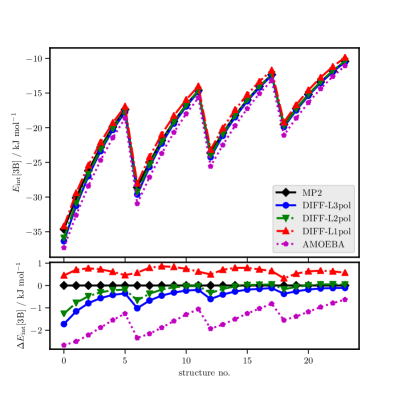
Figure 5: Trimer three-body energies using the three DIFF models as well as the AMOEBA model. Trimer geometries, MP2 and AMOEBA energies are from from Liu et al. Liu et al. (2017). The lower panel displays three-body non-additive energies relative to those from MP2.

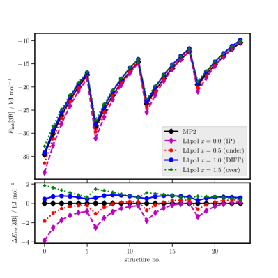
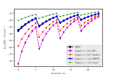
Figure 6: Trimer three-body energies using all seven models. Geometries, MP2 and AMOEBA energies from Liu et al. Liu et al. (2017). For the L1pol models the three-body non-additive energies are also displayed relative to those from MP2.

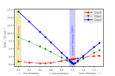
Figure 7: Sensitivity of the 3-body energy of the trimers from the set of Liu et al. Liu et al. (2017) to changes in the damping model. The proposed (DIFF) damping model ($x=1$) is indicated in blue, and the IP-based model ($x=0$) is indicated in yellow.

The water trimers tested thus far are all based on the most stable trimer configuration and all have negative three-body non-additive energies. Akin-Ojo and Szalewicz Akin-Ojo and Szalewicz (2013) have provided a more extensive set of 600 trimers obtained from snapshots taken from a water simulation. These include not only clusters with an attractive 3B contribution, but also those with a repulsive 3B energy, and consequently present a more challenging test for the many-body non-additive models. As with the trimers from Liu et al. (above), the monomer geometries used in this larger set of timers is the same as that used in the construction of the DIFF models.

In Figure 8 we display the 3B non-additive energies from the three DIFF models against the CCSD(T) reference energies from Akin-Ojo and Szalewicz. All three DIFF models show a good correlation with the reference energies, with the scatter progressively decreasing as the maximum rank of the polarizabilities increases. The DIFF models are able to describe the attractive non-additive energies more accurately, with errors increasing for the repulsive energies. However we clearly see that as the rank of the model increases, so does the ability of the model to describe the repulsive non-additive energies: DIFF-L1pol shows sizable scatter and underestimation of the 3B non-additive energy above 1 $\,\rm{kJ\,mol}^{-1}$, but the scatter is reduced in the L2pol and L3pol models which are in good agreement with the CCSD(T) references even for trimers with $E_{\mathrm{int}}\text{[{3}B]}\approx 2$ $\,\rm{kJ\,mol}^{-1}$.

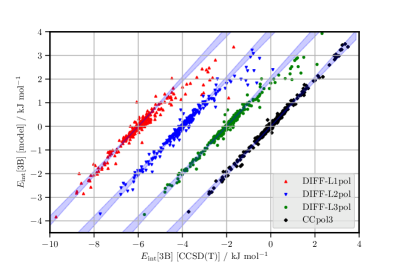
Figure 8: Trimer three-body non-additive energies for the 600 trimer Akin-Ojo & Szalewicz Akin-Ojo and Szalewicz (2013) data set. Comparison is made to the 3B energies from the CCpol23+ model from Góra et al. Góra et al. (2014) Starting from the right, the datasets are offset by multiples of $-2$ $\,\rm{kJ\,mol}^{-1}$ along the $x$-axis.

For comparison we also include the CCpol3 3B model energies in Figure 8. This model, from Góra et al. Góra et al. (2014) is a 12-dimensional three-body non-additive model fitted to 71,000 trimers as described in the Introduction. We can see that while CCpol3 is indeed better than all the DIFF models, it is not significantly better than the DIFF-L3pol model, except for the few trimers with 3B energies larger than 2 $\,\rm{kJ\,mol}^{-1}$. The mean-absolute and root-mean-square errors (MAE and RMSE) for these models are shown in Table 2. The differences in MAEs are quite small, particularly between CCpol3 and DIFF-L3pol. However, the increased overestimation of the 3B energies above 2 $\,\rm{kJ\,mol}^{-1}$ causes an increase in the RMSE in DIFF-L3pol compared with CCpol3. Despite this, it should be evident that if we are concerned primarily with trimers with an attractive or weakly repulsive three-body non-additivity, then the CCpol3 model is comparable in accuracy to the DIFF-L3pol and DIFF-L2pol models. In fact, given that no trimers were used in the determination of any of the DIFF models, their predictive power is remarkable.

The Akin-Ojo and Szalewicz data set is particularly significant as in a detailed study of polarization modelling using the damped Drude oscillator approach, they concluded Akin-Ojo and Szalewicz (2013) that classical polarization models cannot be used to model the non-additive energies in water, particularly the exchange non-additivity. Here we have shown that this is not the case: the classical polarization models we have constructed can all describe the three-body non-additivity, except for the trimers with the most repulsive $E_{\mathrm{int}}\text{[{3}B]}$ energies. Why did Akin-Ojo and Szalewicz come to this perhaps too pessimistic conclusion? Some insight may be obtained from Fig. 1 from their paper, and also from the polarization energy models that are part of CCpol3 and CC-pol-8s. 3B energies from the latter two are visualised in Figure 9. These are both significantly poorer at modelling the reference CCSD(T) 3B energies compared with DIFF-L3pol or even DIFF-L1pol, which is similar in complexity. The MAE/RMSE errors for the CCpol3-3B(pol) and CC-pol-8s-3B(pol) models are shown in Table 2 and these are much larger than those from the DIFF models, in fact, they are substantially larger than those from DIFF-L1pol. It is not clear why the polarization models in the CCpol3 and CC-pol-8s models are not more accurate. It could be the way in which the damping was modelled or the way in which the molecular polarizabilities and multipoles were chosen. But whatever the cause, the poor performance of these models seems to have caused Akin-Ojo and Szalewicz to be over pessimistic about the accuracies that can the attained by a well constructed polarization model, and any of the DIFF models may serve as a counterexample.

Model	MAE	RMSE
DIFF-L1pol	0.091	0.235
DIFF-L2pol	0.064	0.163
DIFF-L3pol	0.058	0.141
Polarization part of CCpol models:
CCpol3-3B(pol)	0.121	0.307
CC-pol-8s-3B(pol)	0.159	0.449
Explicit 3B potentials:
CCpol3	0.042	0.065
CC-pol-8s	0.094	0.175
HBB2-pol	0.082	0.157
WHBB6	0.148	0.269

Table 2: Mean-absolute errors (MAEs) and root-mean-square errors (RMSEs) in 3-body energies for the water models on the 600 trimer data set from Akin-Ojo & Szalewicz Akin-Ojo and Szalewicz (2013). Errors are computed against CCSD(T) references and are reported in $\,\rm{kJ\,mol}^{-1}$. The DIFF models data have been obtained in this work, all other data was obtained from data supplied by Góra et al. Góra et al. (2014).

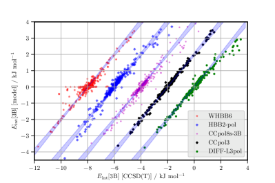
Figure 9: Comparison of the DIFF-L3pol and DIFF-L1pol models with the polarization models from CCpol23+ and CCpol8 (upper panel), and the 3B potentials from HBB2, WHBB6 and CCpol8s (lower panel). Trimer three-body non-additive energies for the 600 trimer Akin-Ojo & Szalewicz Akin-Ojo and Szalewicz (2013) data set. Data for all but the DIFF models was taken from Góra et al. Góra et al. (2014) Starting from the right, the datasets are offset by multiples of $-2$ $\,\rm{kJ\,mol}^{-1}$ along the $x$-axis.

CCpol3 is but one of a group of accurate explicit 3-body non-additive models for water; that is, the 3-body non-additivity is not modelled through a polarization model, but is fit to a functional form to include terms such as the exchange and dispersion non-additivities that a classical polarization model does not include. The CC-pol-8s Cencek et al. (2008), HBB2-pol Medders et al. (2013), and WHBB6 Wang et al. (2011) models are amongst the others in this class of explicit 3-body models, and all are fitted to extensive sets of water trimers. In Figure 9 we compare these models on the 600 water trimers, and MAEs and RMSEs are reported in Table 2. The CCpol3 model is clearly the best able to model the CCSD(T) reference 3B energies, and this is no doubt testimony to its careful parametrization on the extensive set of trimers. With the exception of CCpol3, the DIFF-L3pol and DIFF-L2pol models are better at reproducing the reference 3B energies than any of CC-pol-8s, HBB2-pol or WHBB6. The latter fares substantially worse than DIFF-L1pol. Note that HBB2-pol has been superseded by the MB-pol model which has been demonstrated to significantly outperform HBB2-pol on the water trimers Babin et al. (2014).

V.2 Molecular flexibility and the DIFF models

The comparisons made with the extensive set of trimers was straightforward because both the Liu et al. Liu et al. (2017) and the Akin-Ojo & Szalewicz Akin-Ojo and Szalewicz (2013) datasets used trimers with a fixed monomer geometry that was the same as that used in the DIFF models. For the larger clusters this is not the case. Now the monomers are allowed to relax and so we are led to a question: how are the DIFF models to be used on structures with slightly different molecular conformations?

One solution would be to transform all flexible monomers in a cluster into the rigid monomer geometry used in developing the models. Another solution would be to adapt the rigid body model to the new molecular conformation. The latter approach has the merit that the site-site separations in the cluster are preserved, however, it is not a priori obvious if the interaction model would be well-behaved if the expansion centres were moved relative to each other. To know which of these approaches is best we would need to create a model that includes intramolecular flexibility, but this is not the goal of this paper. Instead we will rely on the fact that the ISA properties — multipole moments and perhaps even the ISA-Pol polarizabilities — do not alter significantly on modest changes to the molecular conformation Verstraelen et al. (2012) and should be transferable onto the molecular conformers without alteration. Additionally, we also move the short-range parameters from the DIFF models onto the new molecular site locations. All DIFF model parameters can be defined in the local-axis framework of the molecule, and this includes the anisotropy parameters. Consequently when the molecular conformation alters and the site locations change, so do the local-axis frames for the three sites in the water molecules. The short-range anisotropy in the Born–Mayer term, as well as the site multipoles and local polarizabilities, all rotate with the local-axis frames. Thus there is a well-defined way of transferring the parameters of any DIFF model onto molecules with different conformations, and as long as these conformations are not too far from the one used in the DIFF model parametrizations, we may expect that the resulting model will result in sensible interaction energies.

Clearly the above premise needs to be systematically tested, but we will simply adopt it here and instead note that we will now expect to see deviations in the cluster energies because of this imposed flexibility of the DIFF models.

One final point: the DIFF models can be used for intermolecular geometry optimizations only. Consequently, when we optimize the clusters geometries, we will do so with the molecular conformations kept fixed. That is, no intramolecular degrees of freedom will be allowed to vary.

V.3 The water hexamers

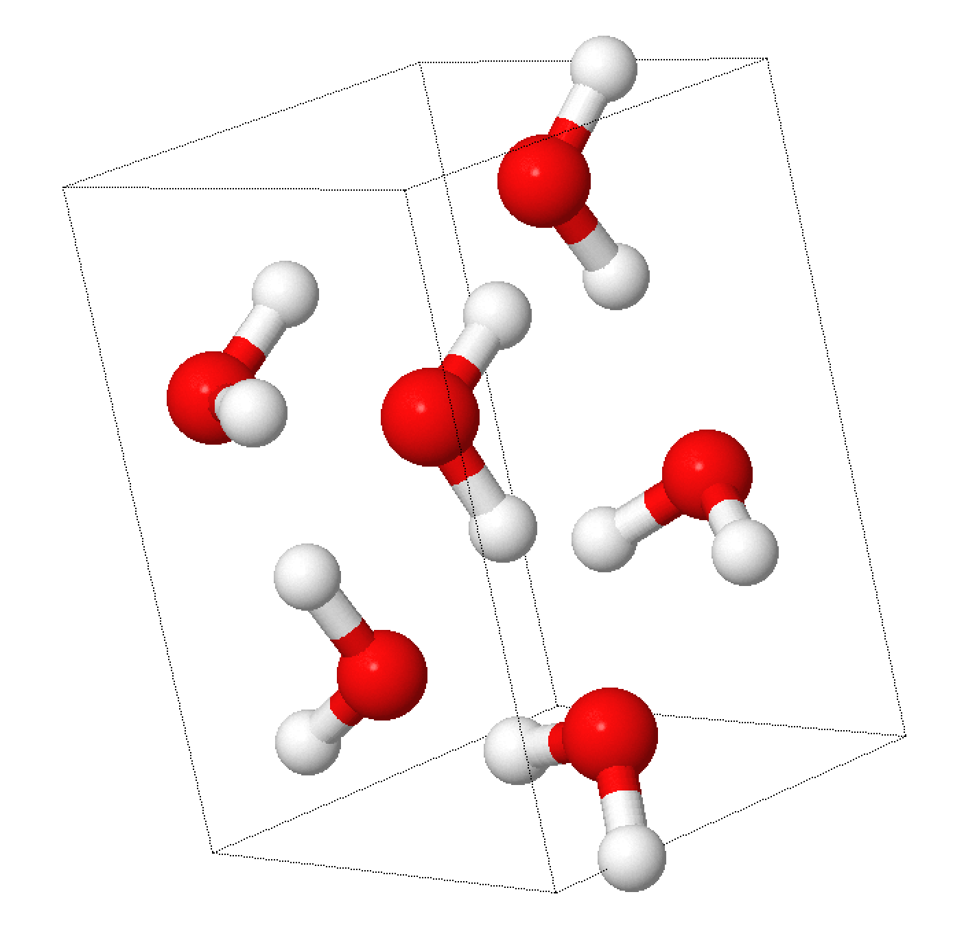
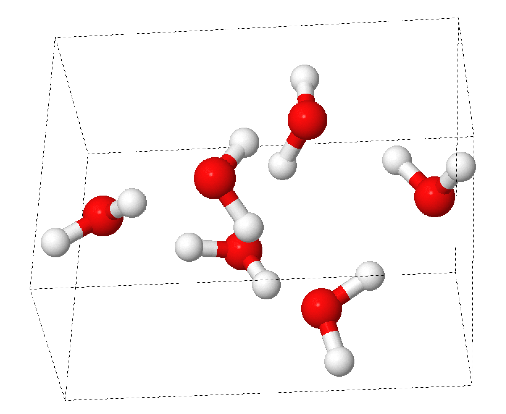
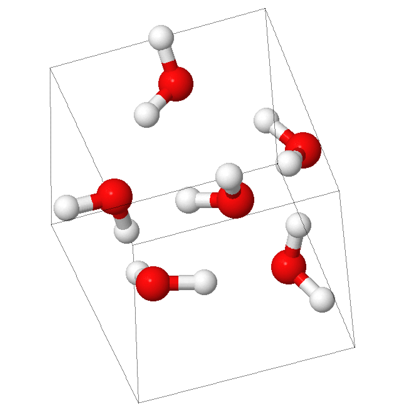
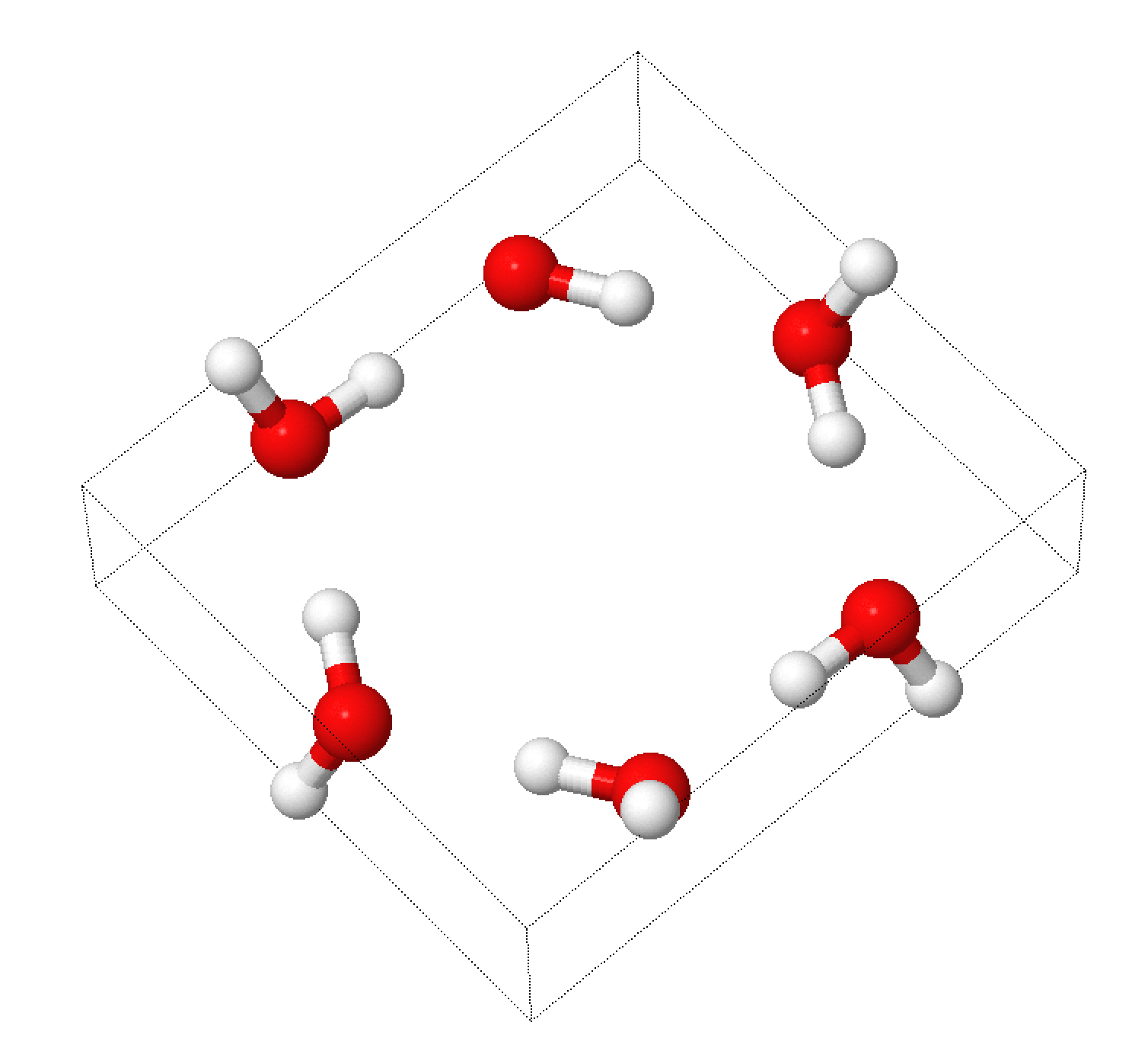
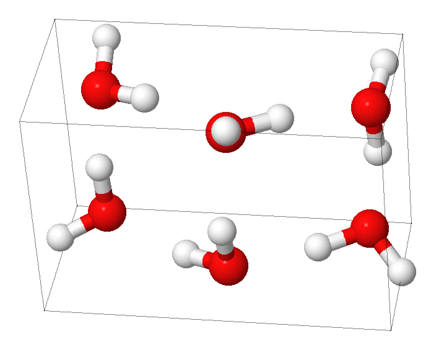
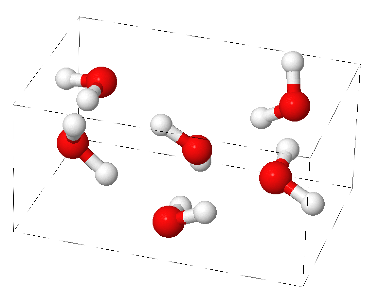
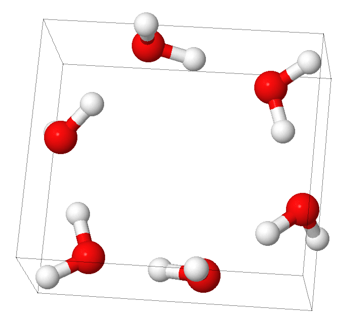
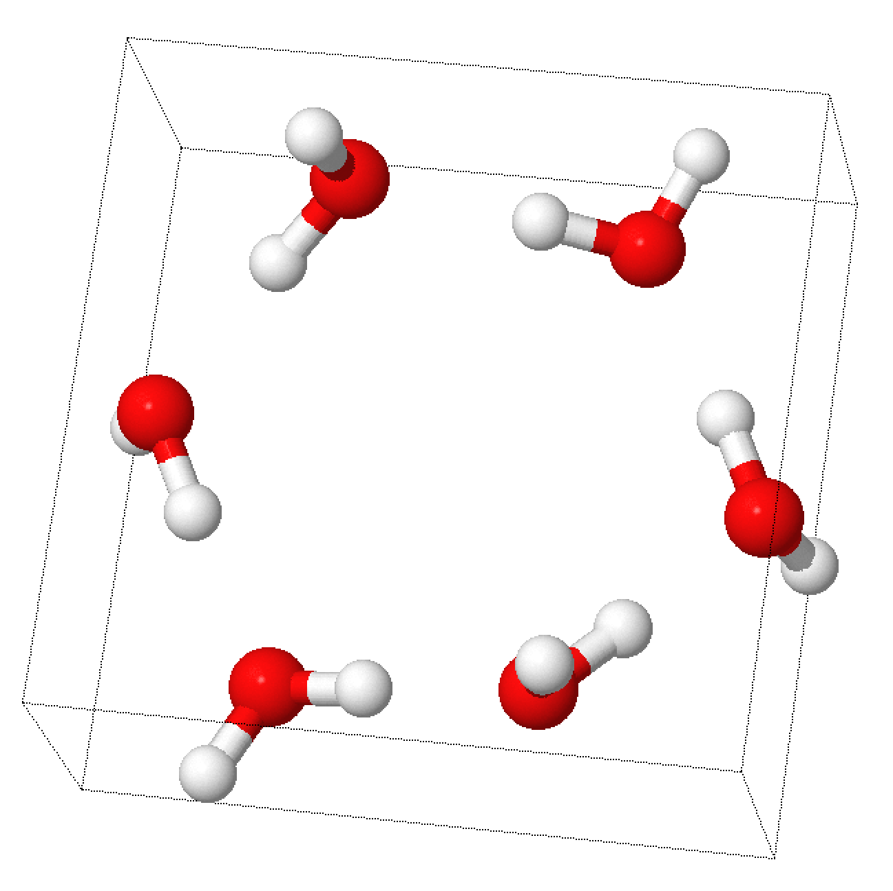
[-5pt](a) prism [-5pt](b) cage [-5pt](c) bag [-5pt](d) cyclic-chair [-5pt](e) book-1 [-5pt](f) book-2 [-5pt](g) cyclic-boat-1 [-5pt](h) cyclic-boat-2

Figure 10: Hexamers used in this study. The structures have been optimized using MP2/CBS by Bates & Tschumper Bates and Tschumper (2009).

The extensive and accurate theoretical data available for the hexamer energies and structures has meant that every ab initio model is tested against the hexamers cis . Additionally, the structural information determined from broadband rotational spectroscopy by Perez et al. Pérez et al. (2012) means that there is a link to experiment even if only some structural data (the O…O separations) are determined with confidence. In this work we use as our references the MP2/CBS optimized hexamer geometries from Bates and Tschumper Bates and Tschumper (2009) which are shown in Figure 10. Reference energies are the CCSD(T)-F12 hexamer energies from Medders et al. Medders et al. (2015), who have also computed the many-body decomposition of the total intermolecular interaction energies of the hexamer isomers, thus allowing a detailed comparison of the DIFF models.

In Figure 11 we display the hexamer intermolecular energies from the DIFF models along with the reference CCSD(T)-F12 energies and those from the MB-pol model Medders et al. (2015). We do not present the hexamer energies with respect to the prism structure energy as is done by many authors, but have instead displayed the absolute intermolecular interaction energies. This is because if the energy of the prism structure happens to be in error, as is the case here, the relative energies will lead to a falsely pessimistic picture. The DIFF-L3pol model gives hexamer energies in good agreement with the CCSD(T)-F12 references with differences in energy of no more than 2 $\,\rm{kJ\,mol}^{-1}$ at the prism and cyclic-boat-1 structures, and less than 1 $\,\rm{kJ\,mol}^{-1}$ for the cage to ring structures. The DIFF-L2pol model shows somewhat larger errors, but here too the maximum error is only just over 2 $\,\rm{kJ\,mol}^{-1}$. On the other hand, while the DIFF-L1pol model shows a remarkable agreement with the reference energies for the prism to bag structures, this model overestimates the binding energies of the ring-like structures. Both DIFF-L2pol and DIFF-L3pol show the correct energetic ordering of the hexamers up to the cyclic boat, but this is not the case for DIFF-L1pol. Notice that both of the higher ranking DIFF models compare favourably to the MB-pol model.

Also shown in Figure 11 are the energies of the hexamers with the intermolecular degrees of freedom relaxed. There are almost no intermolecular geometric changes on the DIFF-L2pol and DIFF-L3pol surfaces, with O…O separations changing no more than $0.03$ Å. This is reflected in the small energetic lowering on optimization on these surfaces. However, for the DIFF-L1pol model the optimized energies can be as much as 2 $\,\rm{kJ\,mol}^{-1}$ lower, and although the O…O separations can alter by only $0.04$ Å (similarly to the higher ranked models), for the more open cyclic-boat structures optimizations using this model leads to structural torsional changes of around 30°, that is, the boat structures invert, while for the DIFF-L2pol and DIFF-L3pol models these changes are only 6° and 3°.

In Figure 12 we display the hexamer energies for the L1pol and L3pol models with the alternative damping models discussed in  §IV.1.3. This is done both for the hexamers at the Bates & Tschumper reference geometries and for the optimized geometries, where optimizations were possible. For both the L1 and L3 polarization models, the DIFF damping models ($x=1.0$) lead to the best agreement with the reference energies. Unlike the case of the trimers (see Figure 6) where the changes in damping model made little difference to the energies from the L1 polarization model, for the hexamers we see considerably more variations in the energies, with the difference in energies between structures increasing as the damping model changes. However, like the case for the trimers, the L3 polarization models show even more sensitivity to the choice of damping, with the accurate DIFF-L3pol model separated from the $x=1.5$ and $x=0.5$ models by around 10 $\,\rm{kJ\,mol}^{-1}$. It is worth recalling that all the models used here were fitted to yield the same two-body energies: they differ only in how they treat the polarization damping, and this difference is magnified substantially in the many-body energies of the clusters. In Figure 13 we display the MAEs for the L1, L2 and L3 polarization models as a function of interpolation parameter $x$. The MAE for the L3 model shows a minimum almost exactly at $x=1.0$, while for the L2 model the minimum occurs just below 1.0, that is slightly less damping may be needed, and for the L1 polarization model there is a broad minimum near $x=1.1$, that is more damping is needed.

The alternate damping models not only lead to different cluster energies, but they can also exhibit very different results for the geometry optimizations of the hexamers. From Figure 12 we see that the IP-based damping ($x=0.0$) for both L1 and L3 polarization models leads to the polarization catastrophe: that is, optimization does not converge and intermolecular bond lengths become arbitrarily small. The moderately underdamped ($x=0.5$) L3 polarization model also results in the polarization catastrophe. The DIFF damping model ($x=1.0$) is optimal for the L3 polarization model and close to optimal for the L1 model. While the overdamped ($x=1.5$) L1 model actually shows better hexamer energy ordering and slightly less structural variations on optimization than the $x=1.0$ DIFF-L1pol model, for the L3 model the structures tend to expand and show increases in the O…O distances of as much as 0.07 Å, with large torsional changes of 45° in the cyclic-boat structures.

Following the discussion in  §V.2, we should expect errors in the energies from the DIFF models as the water conformations in the hexamers are not fixed, but instead vary within and between the hexamer conformers. Additionally, no non-additive dispersion is included in the DIFF models, and although these energies are expected to be small, they are non-negligible Stone (2013) for the more compact hexamers. From Figure 14 we see that this good agreement arises from an error cancellation between the two-body and many-body energies: While the DIFF models are able to predict the overall trends of the $n$-body contributions of the hexamer isomers, they are offset from the reference values. We emphasise that this is not necessarily a deficiency of the DIFF models as these were designed for systems with water molecules held in a fixed geometry. What is remarkable is that these deviations in the $n$-body energies cancel to such a large extent to result in accurate total interaction energies.

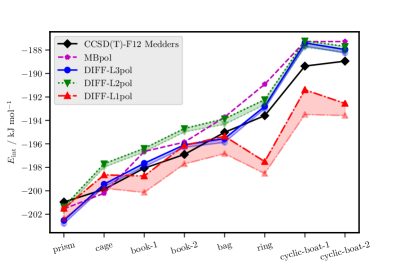
Figure 11: Total interaction energy for hexamers using the DIFF models with maximum polarizabilities of maximum rank 1, 2 and 3, all damped with the proposed ($x=1$) DIFF damping models. For each of the DIFF models the hexamer geometries have been relaxed with the monomers kept rigid. These relaxed interaction energies are indicated by the faded points and lines for each of the DIFF models. Reference interaction energies are the CCSD(T)-F12 energies from Medders et al. Medders et al. (2015). Also shown are the MB-pol interaction energies also taken from Medders et al.. The hexamer geometries are from Bates and Tschumper Bates and Tschumper (2009).

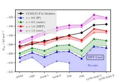
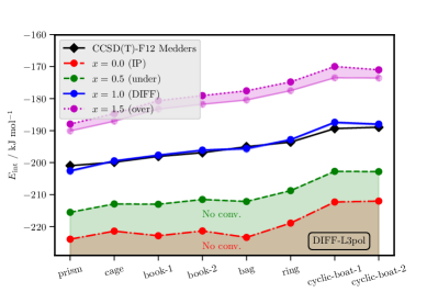
Figure 12: Variations in the hexamer energies as a function of the polarization damping used in the DIFF models. The damping models are obtained using the interpolation scheme discussed in the text. For all DIFF models the solid points indicate interaction energies computed at the reference geometries from Bates and Tschumper Bates and Tschumper (2009). The faded lines and points indicate the energies of the relaxed structures. For some under-damped polarization models the relaxation leads to the polarization catastrophe. In these cases geometry convergence is not achieved and is indicated with ’No conv.’.

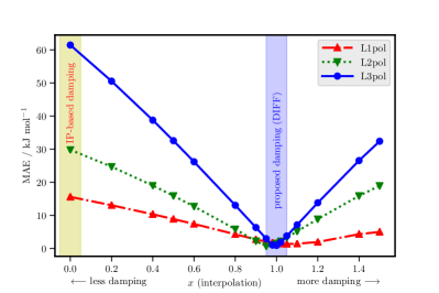
Figure 13: Sensitivity of the many-body polarization energy of the hexamers to changes in the damping model. The proposed damping model ($x=1$) is indicated in blue, and the IP-based model ($x=0$) is indicated in yellow.

Figure 14: $n$-body decomposition of the hexamer energies using the reference geometries from Bates and Tschumper Bates and Tschumper (2009).

V.4 Larger water clusters: 16-mers and 24-mers

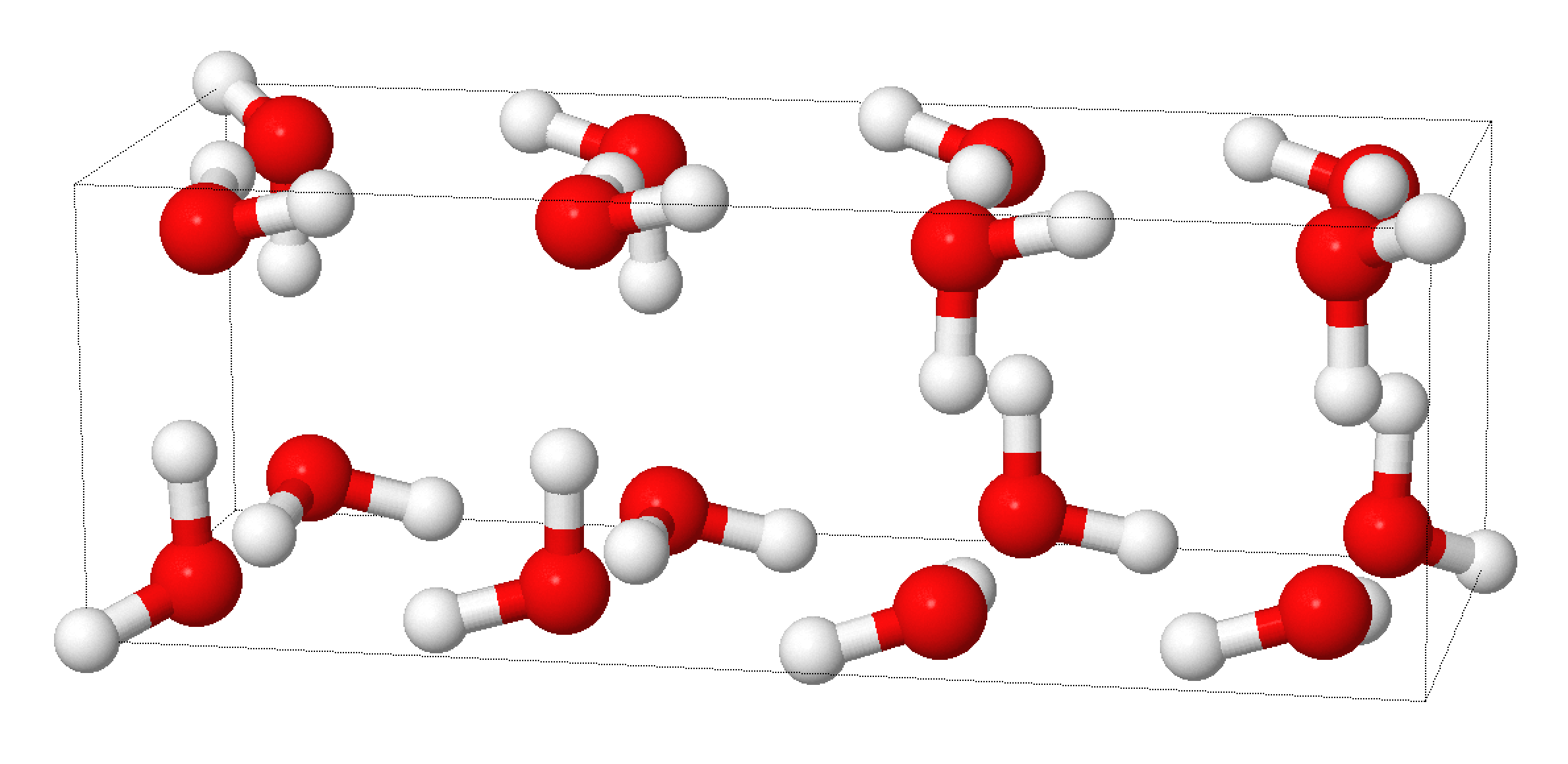
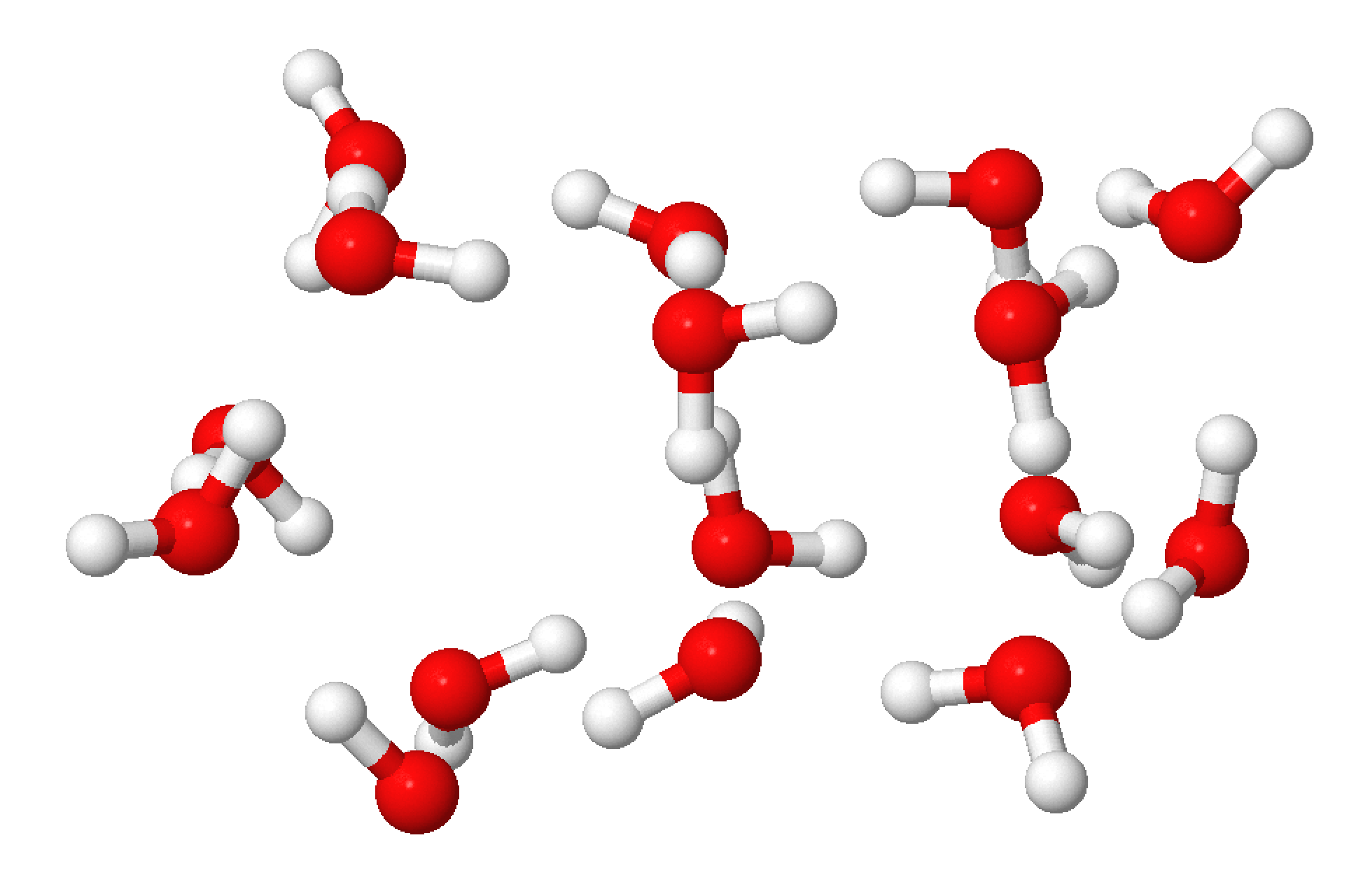
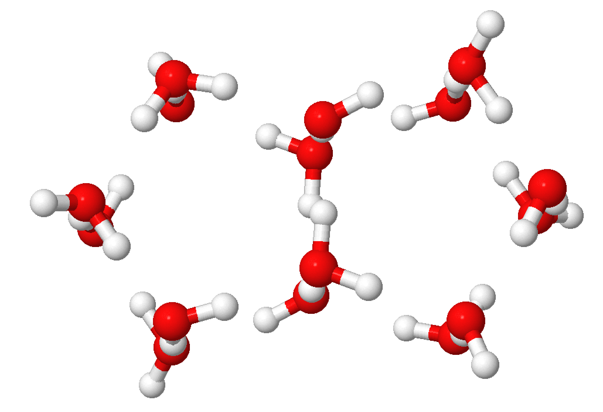
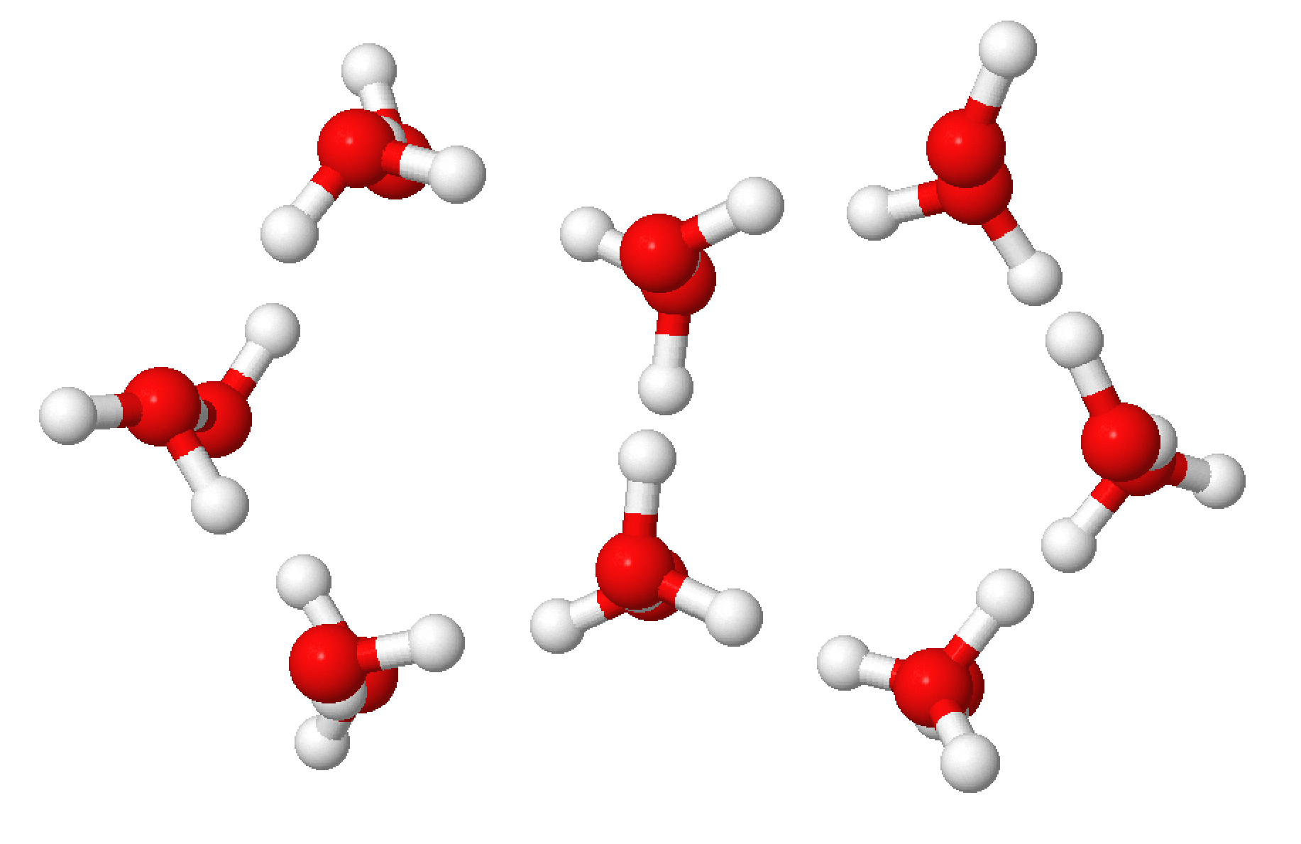
[-5pt](a) 4444-a [-5pt](b) 4444-b [-5pt](c) anti-boat [-5pt](d) boat-a [-5pt](e) boat-b

Figure 15: 16mers used in the study.

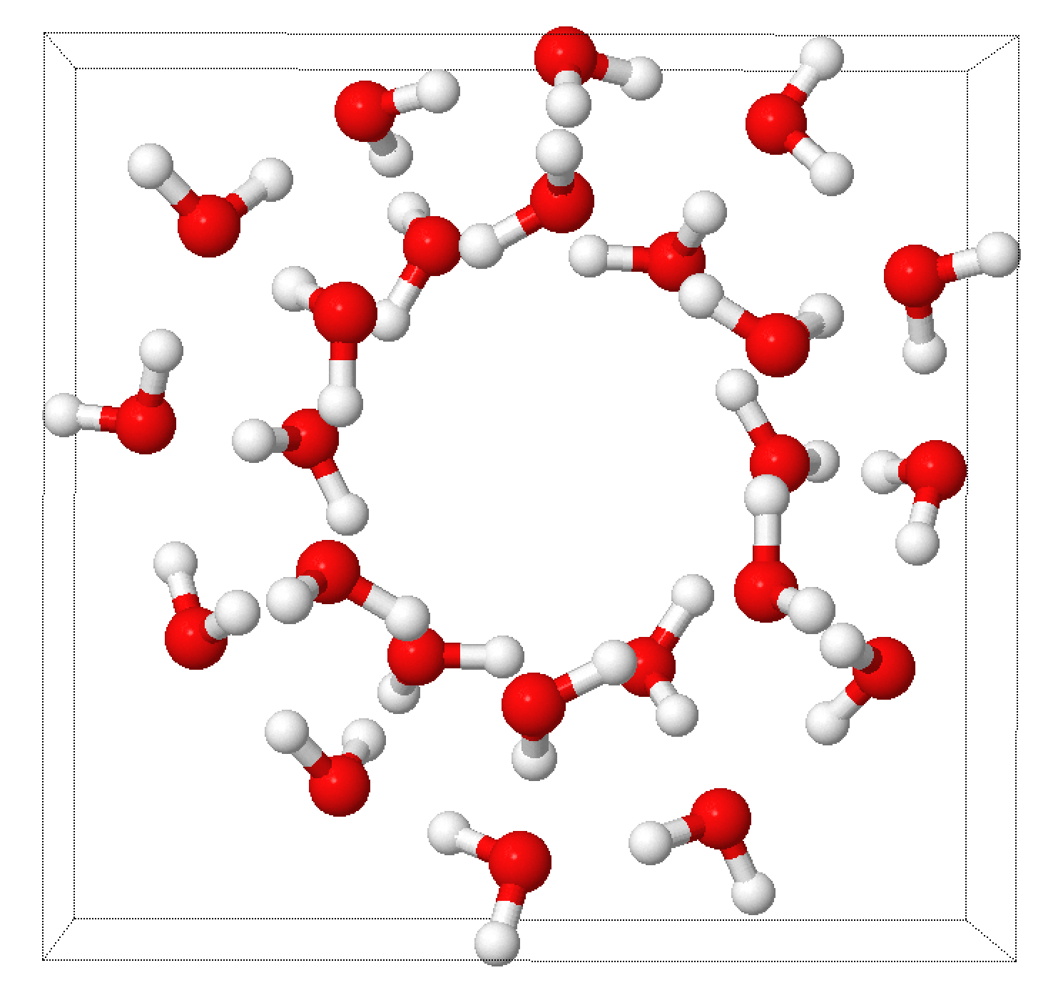
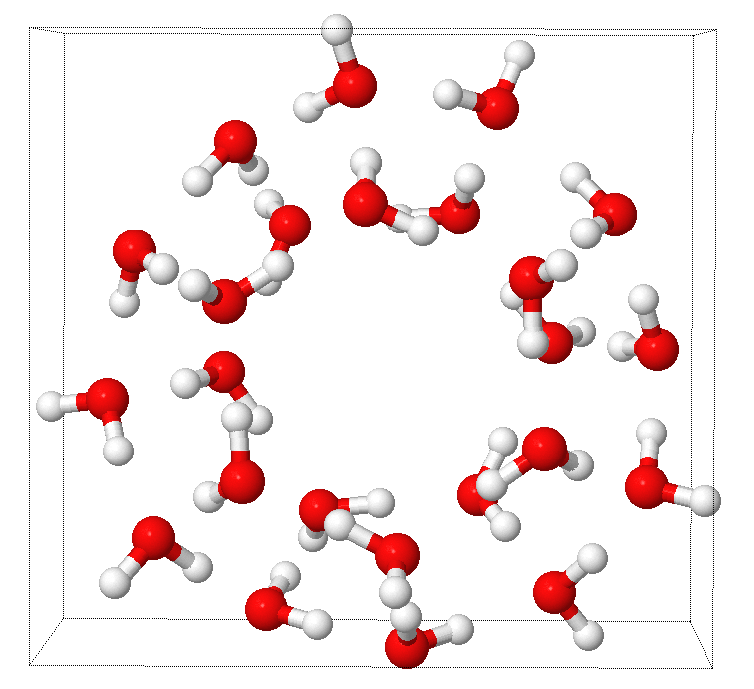
[-1pt](a) 308 [-1pt](b) 316

Figure 16: 24mers used in the study.

In this final set of tests, we will use the DIFF models to evaluate the many-body energies of the larger water clusters shown in Figure 15 and Figure 16. In general, for reasons discussed in  §V.2 and also in  §V.3 we will focus more on trends than actual interaction energies, as these are more likely to be reproduced with models that are not explicitly dependent on the molecular conformations.

V.4.1 (H₂O)₁₆ isomers

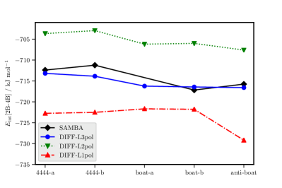
Figure 17: (H₂O)₁₆ isomer interaction energies including two-body to four-body contributions, $E_{\mathrm{int}}\text{[{2}B-{4}B]}$, computed with the three DIFF models and the reference SAMBA energies from Góra et al. Góra et al. (2014). There are no SAMBA references for the boat-a structure. All energies are computed at the reference geometries from Yoo and Xantheas Yoo and Xantheas (2017).

The (H₂O)₁₆ clusters have been optimized by Yoo and Xantheas Yoo and Xantheas (2017) and this set includes two bonding variants of the “4444” structure and two of the “boat” structure. The fifth structure, the “anti-boat”, was estimated Yoo and Xantheas (2017) to have an energy lying between the two boat structures. The best estimates of the energies (total and many-body decomposition) of these clusters (excluding the boat-a isomer) have been obtained by Góra et al. Góra et al. (2014) using the SAMBA algorithm. The SAMBA method avoids energy calculations of the cluster as a whole, but instead makes use of the many-body expansion to arrive at the total interaction energy from a sum of dimer, trimer, and higher-body contributions. In this way, appropriate levels of theory and basis sets can be used for each level, and numerical issues like the basis-set superposition error (BSSE) can be corrected. The intermolecular interaction energies for the (H₂O)₁₆ isomers are given in Table 3 and are terms including 2-body to 4-body contributions, $E_{\mathrm{int}}\text{[{2B-4B}B-{,}B]}$ are displayed in Figure 17. Note that SAMBA reference energies are not available for the boat-a isomer.

The (H₂O)₁₆ isomers have reference energies within only 6 $\,\rm{kJ\,mol}^{-1}$, which is half the energy range of the water hexamers. The 4444-a and 4444-b isomers differ in energy by only 1.2 $\,\rm{kJ\,mol}^{-1}$ and the boat-b and anti-boat isomers differ by 1.4 $\,\rm{kJ\,mol}^{-1}$. However there is a wider gap between the 4444-a/b and boat-b/anti-boat sets which are separated by around 3.4 $\,\rm{kJ\,mol}^{-1}$. Consequently when looking for trends we focus on this larger energy separation as it is less likely to be an artefact of the SAMBA reference energies. First of all, the DIFF-L3pol energies are within 2 $\,\rm{kJ\,mol}^{-1}$ of the SAMBA energies, and the DIFF-L2pol and DIFF-L1pol models are within 10 $\,\rm{kJ\,mol}^{-1}$, with the former underestimating the cluster binding, and the latter leading to an overestimation. Both higher-ranking DIFF models give an acceptable separation of the 4444-a/b and boat-b/anti-boat groups of isomers: for DIFF-L3pol and DIFF-L2pol the separation is 2.6 $\,\rm{kJ\,mol}^{-1}$ and 3.1 $\,\rm{kJ\,mol}^{-1}$, resp., in good agreement with the 3.4 $\,\rm{kJ\,mol}^{-1}$ SAMBA reference. However, the DIFF-L1pol model results in 4444-a/b and boat-b being nearly iso-energetic, and the anti-boat structure being more stable than the boat-b isomer by 7.4 $\,\rm{kJ\,mol}^{-1}$. It is not clear why this is the case, but the problem appears similar to the inability of the DIFF-L1pol model to describe the energetic ordering of the ring-like water hexamers.

Also shown in Table 3 are the interaction energies of the optimized (H₂O)₁₆ isomers on the DIFF surfaces. All isomers are minima on the DIFF-L3pol and DIFF-L2pol surfaces, with very little energetic reduction on optimization, and geometric changes in the O…O separations of order 0.01 Å only. However for the DIFF-L1pol model there are larger geometric changes on optimization with O…O separations changing by as much as 0.04 Å, and energies lowering by between 4 to 8 $\,\rm{kJ\,mol}^{-1}$. This is again similar to the performance of these models on the water hexamers, and once again we observe that the higher ranking polarization models seem better able to describe both the energies and structures of the water clusters.

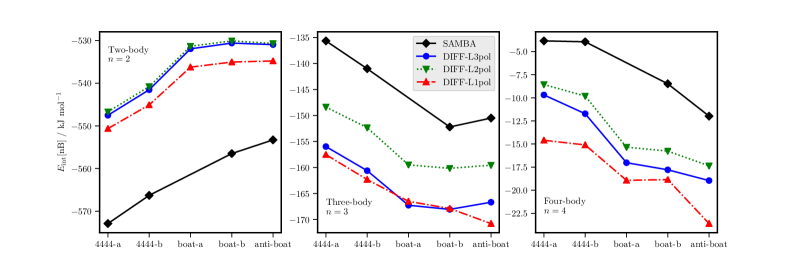
Figure 18: Comparison of the $n$-body energies from the DIFF models with the SAMBA references from Góra et al. Góra et al. (2014). There are no SAMBA references for the boat-a structure.

In Figure 18 we display the many-body energy decomposition of the (H₂O)₁₆ clusters. As with the hexamers (see Figure 14) we see that the excellent total interaction energies from the DIFF models results from a cancellation of errors made in the 2-body and many-body energies. The general trends in the DIFF-L2pol and DIFF-L3pol $n$-body energies are very similar to those from the SAMBA references, but the DIFF-L1pol model shows a comparative over-estimation of the anti-boat many-body energies. Part of the overestimation of the many-body energies results from the use of molecular properties evaluated at the reference monomer geometry and transferred to the flexible monomers in the clusters. We have made an estimate of the magnitude of this effect by evaluating the molecular properties at the water equilibrium geometry rather than at the vibrationally averaged geometry used in the DIFF models. This change results in 3-body energies that are around 5 $\,\rm{kJ\,mol}^{-1}$ smaller (in magnitude) than those from the DIFF models, and brings them closer to the SAMBA references. The main effect arises from the change in the water multipoles, with the changes in the polarizabilities having a smaller impact on the energies. A more systematic study of this effect is needed and is in progress in our group.

V.4.2 (H₂O)₂₄ isomers

The two (H₂O)₂₄ isomers shown in Figure 16 are the largest clusters considered in this study. SAMBA reference energies for these clusters Góra et al. (2011) show that the 308 and 316 isomers are nearly isoenergetic, with an $E_{\mathrm{int}}\text{[{2}B-{4}B]}$ energy difference of less than 1 $\,\rm{kJ\,mol}^{-1}$, and the 308 isomer the more stable. This small difference arises from a near cancellation of energy differences in the 2B and 3B energies of the two isomers. From Table 20 in the SI we see that at the 2B level, 308 is more stable by around 7 $\,\rm{kJ\,mol}^{-1}$, but at the 3B and 4B levels it is less stable by around 5 $\,\rm{kJ\,mol}^{-1}$ and 1 $\,\rm{kJ\,mol}^{-1}$. Therefore, these clusters present a good test of the balance between the two-body and many-body parts of the interaction models.

In Figure 19 we display the differences in the model energies from the SAMBA references. Here we consider the DIFF as well as CCpol23+ and CC-pol-8s-NB models with data for the latter two taken from Góra et al. Góra et al. (2014). All models show almost exactly the same errors for the 2-body energies, but the DIFF models show smaller errors for the 3-body non-additivity, and the CC models show smaller errors for the 4-body non-additivity. As the errors made by the DIFF models for the 2-body and many-body energies are of opposite signs, these largely cancel out to result in better agreement than the two CC models with the SAMBA references for the $E_{\mathrm{int}}\text{[{2}B-{4}B]}$ estimate of the cluster interaction energies. This was not expected as CCpol23+ is based on CCSD(T) reference energies as are the SAMBA references, but the DIFF models are based on SAPT(DFT) references.

Also shown in Figure 19 are the relative energy differences, $\Delta E_{\mathrm{int}}$, between the 316 and 308 isomers from the SAMBA reference calculations and the DIFF and CC models. These are displayed both for $E_{\mathrm{int}}\text{[{2}B-{4}B]}$ as well as for the individual contributions from the many-body expansion. All models underestimate the 2-body contribution to $\Delta E_{\mathrm{int}}$, but the CC models and the DIFF-L1pol model show better agreement with the 3-body contribution to the energy difference, while the two higher-ranking DIFF models underestimate this difference. On the other hand, at the 4-body level the DIFF-L2pol and DIFF-L3pol models show an excellent agreement with the SAMBA references, while the CC and DIFF-L1pol models predict an energy difference of the wrong sign. All models show excellent agreement with the very small total isomer interaction energy difference, $\Delta E_{\mathrm{int}}\text{[{2}B-{4}B]}$, with the CCpol23+ and CC-pol-8s-NB models closer than the DIFF-L2pol and DIFF-L3pol models. Góra et al. Góra et al. (2014) have made comparisons of the WHBB and HBB2-pol models for these isomers and while HBB2-pol gives energies in reasonably good agreement with SAMBA, the WHBB models (of order 5 and 6) both result in very large errors of around 50 $\,\rm{kJ\,mol}^{-1}$ in the 3-body contribution to $\Delta E_{\mathrm{int}}$. This is well in excess of the 2–3 $\,\rm{kJ\,mol}^{-1}$ errors made by the CC and DIFF models.

We must not place too much importance to the relatively small differences in the CCpol23+, CC-pol-8s-NB and the three DIFF models as all have been transferred onto the flexible water conformers in these (H₂O)₂₄ clusters, so some differences must be expected. Indeed, a perfect agreement would be surprising. Nevertheless, the fact that these differences are so small is remarkable, particularly for the DIFF models which have bee constructed from 1-body and 2-body data only.

Structure	4444-a	4444-b	boat-a	boat-b	anti-boat
SAMBA
$E_{\mathrm{int}}\text{[{2}B-{4}B]}$	-712.397	-711.234	—	-717.179	-715.765
DIFF-L3pol
$E_{\mathrm{int}}\text{[{2}B-{4}B]}$	-713.187	-713.873	-716.235	-716.447	-716.603
$E_{\rm int}$ (Ref geom)	-710.068	-711.449	-714.616	-715.063	-715.107
$E_{\rm int}$ (Opt geom)	-711.239	-712.59	-715.833	-716.342	-716.846
$\Delta E_{\rm int}$	-1.171	-1.141	-1.217	-1.279	-1.739
DIFF-L2pol
$E_{\mathrm{int}}\text{[{2}B-{4}B]}$	-703.661	-702.952	-706.192	-706.014	-707.615
$E_{\rm int}$ (Ref geom)	-700.786	-700.355	-704.446	-704.014	-706.119
$E_{\rm int}$ (Opt geom)	-701.301	-701.364	-704.971	-704.993	-707.125
$\Delta E_{\rm int}$	-0.515	-1.009	-0.525	-0.979	-1.006
DIFF-L1pol
$E_{\mathrm{int}}\text{[{2}B-{4}B]}$	-722.757	-722.513	-721.682	-721.782	-729.189
$E_{\rm int}$ (Ref geom)	-721.556	-721.494	-721.174	-721.041	-729.827
$E_{\rm int}$ (Opt geom)	-725.641	-725.865	-727.392	-728.978	-737.026
$\Delta E_{\rm int}$	-4.085	-4.371	-6.218	-7.937	-7.199

Table 3: Many-body intermolecular interaction energies for (H₂O)₁₆ clusters. The SAMBA reference energies including contributions from 2-body to 4-body interactions, $E_{\mathrm{int}}\text{[{2}B-{4}B]}$, are from Góra et al. Góra et al. (2011). For the DIFF models we report both $E_{\mathrm{int}}\text{[{2}B-{4}B]}$ as well as the total intermolecular interaction energy $E_{\rm int}$ at the reference geometries (“Ref geom”), as well as $E_{\rm int}$ for the optimized cluster geometries with intramolecular conformations fixed as described in  §V.2 (“Opt geom”). $\Delta E_{\rm int}$ is the difference in energies of the optimized and reference structures. All energies are in $\,\rm{kJ\,mol}^{-1}$.

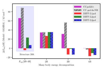
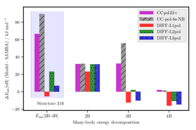
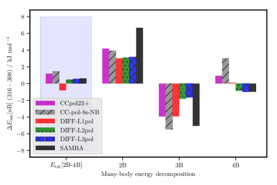
Figure 19: Two-, three- and four-body contributions to the (H₂O)₂₄ dodecahedra 316 and 308 measured relative to SAMBA reference energies from Góra et al. (2011), and the difference in energy between them. Note that there is an error in the SAMBA estimate of $\Delta E_{\mathrm{int}}\text{[{2}B-{4}B]}$ as reported in Table. VI from Góra et al. Góra et al. (2014). This has been corrected in this figure.

VI Analysis

We began this paper with three questions that can now be answered:

• Q1: Can many-body polarization models be developed from the properties of the monomer and dimer energy calculations only?
  Many-body polarization models can be developed from monomer properties and dimer interaction energies alone. The route to this is to use monomer distributed multipoles computed using the basis-space implementation of the iterated stockholder atoms (BS-ISA) algorithm Misquitta et al. (2014), and the monomer distributed polarizabilities computed using the ISA-Pol algorithm Misquitta and Stone (2018a). Additionally and perhaps most importantly, the damping needed for the polarization model needs to be determined using the true polarization energies, as defined using Reg-SAPT(DFT) Misquitta (2013), that are free from charge-delocalization contributions. These models have been demonstrated to reproduce the geometries and energies of a large number of water clusters to an accuracy that rivals that attained by models fitted to extensive sets of water clusters.

• Q2: Can we develop a systematic hierarchy of polarizability model of increasing rank, and how do the accuracies of these models vary with rank?
  The ISA-Pol polarizabilities can be defined at any rank (currently to a maximum of rank 3) and include anisotropy and full coupling within the molecule (all many-body interactions within the molecule are accounted for). We have developed three DIFF models using these polarizabilities of maximum ranks 1, 2 and 3, and have demonstrated that all result in accurate predictions for the energetics of the water clusters, with the higher ranking models also able to accurately reproduce the geometries of the water clusters. Although we have used terms of the same rank on all sites, it is possible to create ISA-Pol models of lower ranks on some sites (say the hydrogen ions), and even to make the polarizability tensors isotropic.

• Q3: How accurate are the damping models obtained from Reg-SAPT(DFT) and how sensitive are the many-body energies and cluster geometries to deviations from them?
  We have shown that the polarization damping models determined using Reg-SAPT(DFT) are close to optimal in the sense that they lead to three-body non-additive polarization energies which are able to describe the MP2 and CCSD(T) reference energies for more than 600 trimers. Additionally, these models show very small errors for the total interaction energies of the water hexamers. Deviating from these proposed damping models leads to increases in errors that are most notable in the models with rank 2 and 3 polarizabilities.

We have demonstrated that the DIFF models, in particular the DIFF-L2pol and DIFF-L3pol models, lead to many-body interaction energies that are comparable in accuracy to the best ab initio water models currently available. These include the recently developed CCpol23+ model Góra et al. (2014) and HBB2-pol Medders et al. (2015) models, as well as more established WHBB model Wang et al. (2011). These three have dedicated three-body models, with additional many-body non-additive effects described through a polarization model. The three-body models in these potentials are fitted to sizeable sets of water trimers, and contain considerable numbers of fitted parameters. Nevertheless, using a set of 600 water trimers extracted from simulations of liquid water Akin-Ojo and Szalewicz (2013) we have demonstrated that the DIFF-L2pol and DIFF-L3pol models are second in accuracy only to the CCpol23+ model (MB-pol was not considered in this comparison and we expect it to equal or surpass CCpol23+ in accuracy). All DIFF models show an increase in errors only for the trimers with the most repulsive three-body non-additive energies (with $E_{\mathrm{int}}\text{[{3}B]}\geq 2$ $\,\rm{kJ\,mol}^{-1}$), for which physical effects not included in the polarization models are expected to be important. As this high accuracy is attained with models built largely from properties computed from the monomers, with only three parameters fitted to a small number of dimer energies, the DIFF approach may be a better route to the development of high-accuracy many-body models in systems with strong many-body polarization. Additional effects may be absorbed in a correction model which could be simpler in structure than the full three-body interaction model.

We have additionally demonstrated how the DIFF models can maintain a high accuracy even when transferred onto systems with flexible water molecules. This high accuracy in the total interaction energy seems to arise from a systematic cancellation of errors in the two-body and many-body energies from the DIFF models. It is not clear why this error cancellation is so systematic, or indeed if it is a feature of water models only (due to the fairly limited bonding types in the water clusters) or is more general. It is possible that the high transferability of the ISA-based monomer properties, in particular the ISA multipoles, may be the reason for the high degree of transferability of the DIFF models. We have already demonstrated that the ISA multipoles do possess a good degree of transferability on molecular crystals Aina et al. (2019), and work is in progress in our group to make an analysis of the ISA-Pol dispersion and polarizability models.

There are also questions which have arisen during the course of this investigation that require further investigation. Perhaps the most important of these

• How should the many-body polarization models of increasing rank be systematically constructed so as to be consistent?

• What is the minimum rank of the polarizability tensor needed to achieve a high accuracy both in the many-body interaction energies and in the cluster geometries. We have shown that the L1pol model is acceptable for the energetics, but perhaps not for the geometries. The L2pol (including quadrupole–quadrupole polarizabilities) were needed for accurate geometries. But is this generally the case, and if so, on which atomic sites are these terms needed?

• The damping models rely on true polarization energies defined using Reg-SAPT(DFT), but this theory relies on a regularization parameter — which defines a length scale — to separate the polarization and charge-delocalization components of the (second-order) induction energy. How sensitive are the DIFF models to the choice of this parameter, and how does this parameter vary with system and atom type?

We have thus far constructed the three DIFF models of maximum polarizability ranks 1, 2 and 3, independently, with the polarization damping models determined separately for each. In this way, the weaker damping for the DIFF-L1pol model makes up for the missing higher-ranking terms, but it is also possible that the resulting larger induced dipoles cause the slight over-binding seen in the ring-like hexamers and the 16-mers. An alternative would be to determine the polarization damping model for the highest ranking polarization model, and then to construct the lower ranking models with the damping kept fixed. This method may have the merit of leading to a more systematic behaviour of the DIFF models as a function of the rank of the polarizability tensors. We are currently investigating this possibility.

While the energetics of the models are important, their performance in determining the structures of the water clusters are equally or perhaps even more important. Both the DIFF-L2pol and DIFF-L3pol models have been shown to result in cluster geometries that agree with the theoretical benchmarks to a very high accuracy: both models result in optimized (intermolecular coordinates only) clusters with O…O separations and important structural angles and torsions in very close agreement with the reference geometries. However the DIFF-L1pol model allows for larger cluster geometry variations when optimizations are performed: O…O separations can change by as much as 0.04 Å and, more importantly, torsional changes can be as much as 30°. It is possible that the cluster geometries are sensitive to the induced quadrupole that arise from the rank 2 polarizabilities and the coupling terms between the rank 1 and 2 terms. If so, this would have important consequences for the development of force-fields. However it is also possible that this sensitivity has arisen because of the way in which the DIFF-L1pol model was constructed, as discussed above. An in-depth analysis of the magnitude of the induced dipoles and quadrupoles would be needed to resolve this puzzle.

Reg-SAPT(DFT), which is crucial in the algorithm used to determine the polarization damping (see  §IV.1), involves one free parameter ($\eta$), and while this parameter was carefully determined by Misquitta Misquitta (2013), it is possible that the choice $\eta=3.0$ a.u. is close to, but not optimal. In fact, $\eta$ may vary somewhat with system and even with atom-types. Any change in $\eta$ would result in a slightly different partitioning of the $E^{(2)}_{\rm IND}$ energy into the second-order polarization and second-order charge-delocalization energies, and this would alter the polarization model damping, and consequently the many-body energies would change. The already excellent agreement of the DIFF model energies with the reference energies on the wide range of water clusters studied here strongly suggests that, at least for water, the regularization used is appropriate. Nevertheless, as we seek to reach ever higher accuracies, we will also need to determine this parameter with a higher degree of confidence, and also investigate how it varies with molecules and atomic sites within a molecule.

VII Conclusions

We set out to determine whether many-body non-additive polarization effects could be determined from models constructed using monomer properties and dimer energies only, and have demonstrated that this is indeed possible. Using ISA-based molecular properties (multipoles and polarizabilities), we have constructed three DIFF (derived intermolecular force-field) models for water that differ in the maximum ranks of the polarization tensors and the polarization damping models only, and have demonstrated that all three models are able to predict the many-body non-additive energies of extensive sets of water trimers, the water hexamers, 16-mers and 24-mers. Additionally, these models are able to correctly describe the intermolecular geometries of the water clusters even when used on clusters with flexible water molecules. We have further demonstrated that while the DIFF-L1pol model (with rank 1 polarizabilities) is relatively less sensitive to the choice in damping model, the two DIFF models with higher ranking polazization tensors are very sensitive to the polarization damping. Further, for all three DIFF models, the optimal polarization damping model was determined from two-body true polarization energies determined using Reg-SAPT(DFT).

The three DIFF models presented in this paper were never meant to be reference models for water, and indeed we have not yet used any in simulations of the liquid, but we have successfully demonstrated that they rival some of the most elaborately parametrized water models, including HBB2-pol Medders et al. (2013), WHBB Wang et al. (2011), MB-pol Babin et al. (2013, 2014), as well as the CC-pol-8s-NB Cencek et al. (2008) and recently developed CCpol23+ Góra et al. (2014) models. Perhaps more importantly for model building, while these models are all built on extensive sets of water trimers and even larger clusters, the DIFF models use only 1-body and 2-body data, in effect reversing a recent trend to large and computationally demanding data sets Ouyang and Bettens (2015). Additionally, the many-body part of the DIFF models for H₂O contains precisely three independent fitted parameters that are determined using a small number of dimer calculations using Reg-SAPT(DFT) Misquitta (2013). The key to the performance of the DIFF models lies in the physical insight used to understand the origin of the many-body polarization, and not in simply fitting to ever-increasing data sets.

In demonstrating the above we have used models based entirely on SAPT(DFT) and Reg-SAPT(DFT), with molecular properties computed using the BS-ISA and ISA-Pol algorithms. These methods are computationally efficient and can be applied to systems much larger than water, and consequently these many-body polarization models can be constructed for larger system too. Indeed we have already done so for the pyridine complex Misquitta and Stone (2016) and have demonstrated that these models lead to the correct description of the structures of the known polymorphs of pyridine, including a new high-pressure phase Aina et al. (2017). While more systems are needed to be sure of the applicability of the methodology, the strong physical underpinning of the methods described in this paper (and in previous papers from our group) leads us to be optimistic that the approach described here is robust and may well be a general route to developing many-body non-additive polarization models that exceed the accuracy of any proposed so far. We note here that there is no real difficulty in combining the DIFF methodology with reference properties and dimer energies from more advanced methods. Indeed the present DIFF models for water all exhibit a mild underbinding of the dimers due to the use of SAPT(DFT) references, and they could be easily improved using CCSD(T) references.

The price to pay for the methodology used in the DIFF models is that the polarization models are more complex and necessitate the development of simulation tools that can handle the many-body polarization in the condensed phase in a computationally efficient manner. The theoretical framework needed for the DIFF models is well known Stone (2013) and has been implemented in the Orient program Stone et al. (2019), but the naïve implementation of the classical polarization model is computationally inefficient. Considerable progress has been made in improving the efficiency of the polarization models, most notably by Lagardere et al. Lagardère et al. (2017) and by Albaugh & Head-Gordon Albaugh and Head-Gordon (2017). However neither of these approaches is directly suitable for even the simplest of the DIFF models. Nevertheless there is nothing fundamental that stops us from improving the flexibility and the computational efficiency of the classical polarization models in simulation codes. And now that we can develop accurate polarization models more readily, it is time we addressed this deficiency in our computational tools and made the necessary effort to allow simulations with theoretically motivated force-fields rather than force theorists to simplify the models and thereby lose in accuracy. That said, it may still be possible to use force-matching methods Salanne et al. (2012); Iuchi et al. (2007) to construct simpler force-fields that are rigorously linked to the underlying theoretical models (such as DIFF). Clearly there are possibilities for moving the DIFF models to mainstream simulations.

VIII Acknowledgements

RAJG thanks Queen Mary University of London and the EPSRC for a studentship that has funded part of this work. AJM additionally thanks the Thomas Young Centre for Theory and Simulation of Materials for a stimulating environment. We thank Krzysztof Szalewicz for helpful comments on parts of this work. We thank Nohad Gresh and Jean-Philip Piquemal for many useful discussions on polarization, charge-delocalization and water models. Finally we acknowledge a considerable gratitude to Anthony J. Stone for a long collaboration which has led to the models discussed in this paper. We thanks the Royal Society for an International Exchange grant IEC$ρ^{2}$81027 that was used to fund some of this work.

IX Additional information

All developments have been implemented in a developer’s version of the CamCASP 6.0 Misquitta and Stone (2018b) program which may be obtained from the authors on request. CamCASP has been interfaced to the DALTON 2.0 (2006 through to 2015), NWChem, GAMESS(US) , and Psi4 programs.

The specifications of the DIFF models are presented in the Supplementary Information. Additionally we supply input files suitable for use with the Orient 5.0 Stone et al. (2019) program which can be freely obtained. We also supply the structures of all water clusters used in this paper so that comparisons can be made easily should the need arise.

References

- Welch et al. (2008) G. W. A. Welch, P. G. Karamertzanis, A. J. Misquitta, A. J. Stone, and S. L. Price, J. Chem. Theory Comput. 4, 522 (2008).
- Cooper et al. (2008a) T. G. Cooper, K. E. Hejczyk, W. Jones, and G. M. Day, J. Chem. Theory Comput. 4, 1795 (2008a).
- Price et al. (2010) S. L. Price, M. Leslie, G. W. A. Welch, M. Habgood, L. S. Price, P. G. Karamertzanisc, and G. M. Day, Phys. Chem. Chem. Phys. 12, 8478 (2010).
- Misquitta et al. (2008a) A. J. Misquitta, G. W. A. Welch, A. J. Stone, and S. L. Price, Chem. Phys. Lett. 456, 105 (2008a).
- Bukowski et al. (2007) R. Bukowski, K. Szalewicz, G. C. Groenenboom, and A. van der Avoird, Science 315, 1249 (2007).
- Jankowski and Szalewicz (1998) P. Jankowski and K. Szalewicz, J. Chem. Phys. 108, 3554 (1998).
- Groenenboom et al. (2000) G. C. Groenenboom, E. M. Mas, R. Bukowski, K. Szalewicz, P. E. S. Wormer, and A. van der Avoird, Phys. Rev. Lett. 84, 4072 (2000).
- van der Avoird et al. (2010) A. van der Avoird, R. Podeszwa, K. Szalewicz, C. Leforestier, R. van Harrevelt, P. R. Bunker, M. Schnell, G. von Helden, and G. Meijer, Phys. Chem. Chem. Phys. 12, 8219 (2010).
- Vissers et al. (2005) G. W. M. Vissers, A. Hesselmann, G. Jansen, P. E. S. Wormer, and A. van der Avoird, J. Chem. Phys. 122, 054306 (2005).
- Misquitta and Stone (2016) A. J. Misquitta and A. J. Stone, Journal of Chemical Theory and Computation 12, 4184 (2016), pMID: 27467814, https://doi.org/10.1021/acs.jctc.5b01241 .
- Stone and Misquitta (2007) A. J. Stone and A. J. Misquitta, Int. Revs. Phys. Chem. 26, 193 (2007).
- Van Vleet et al. (2016) M. J. Van Vleet, A. J. Misquitta, A. J. Stone, and J. R. Schmidt, Journal of Chemical Theory and Computation 12, 3851 (2016), pMID: 27337546, https://doi.org/10.1021/acs.jctc.6b00209 .
- Van Vleet et al. (2018) M. J. Van Vleet, A. J. Misquitta, and J. R. Schmidt, Journal of Chemical Theory and Computation 14, 739 (2018).
- Metz et al. (2016) M. P. Metz, K. Piszczatowski, and K. Szalewicz, Journal of Chemical Theory and Computation 12, 5895 (2016).
- Uteva et al. (2017) E. Uteva, R. S. Graham, R. D. Wilkinson, and R. J. Wheatley, The Journal of Chemical Physics 147, 161706 (2017).
- Li et al. (2017) Y. Li, H. Li, F. C. Pickard, B. Narayanan, F. Sen, M. K. Y. Chan, S. Sankaranarayanan, B. R. Brooks, and B. Roux, J. Chem. Theory Comput. (2017), 10.1021/acs.jctc.7b00521.
- Popelier (2015) P. L. A. Popelier, Int. J. Quantum Chem. 115, 1005 (2015).
- Cooper et al. (2008b) T. G. Cooper, K. E. Hejczyk, W. Jones, and G. M. Day, J. Chem. Theory Comput. 4, 1795 (2008b).
- Harder et al. (2009) E. Harder, A. D. MacKerell, and B. Roux, J. Am. Chem. Soc. 131, 2760 (2009).
- Misra and Blankschtein (2017) R. P. Misra and D. Blankschtein, J. Phys. Chem. C 121, 28166 (2017).
- (21) .
- Stone (2013) A. J. Stone, The Theory of Intermolecular Forces, 2nd ed. (Oxford University Press, Oxford, 2013).
- Babin et al. (2013) V. Babin, C. Leforestier, and F. Paesani, Journal of chemical theory and computation 9, 5395 (2013).
- Babin et al. (2014) V. Babin, G. R. Medders, and F. Paesani, Journal of chemical theory and computation 10, 1599 (2014).
- Kumar et al. (2010) R. Kumar, F.-F. Wang, G. R. Jenness, and K. D. Jordan, The Journal of chemical physics 132, 014309 (2010).
- Millot et al. (1998) C. Millot, J.-C. Soetens, M. T. C. M. Costa, M. P. Hodges, and A. J. Stone, J. Phys. Chem. A 102, 754 (1998).
- Misquitta et al. (2014) A. J. Misquitta, A. J. Stone, and F. Fazeli, J. Chem. Theory Comput. 10, 5405 (2014).
- Misquitta and Stone (2018a) A. J. Misquitta and A. J. Stone, Theor Chem Acc 137, 153 (2018a).
- Lillestolen and Wheatley (2008) T. C. Lillestolen and R. J. Wheatley, Chem. Commun. 2008, 5909 (2008).
- Misquitta (2013) A. J. Misquitta, J. Chem. Theory Comput. 9, 5313 (2013).
- Aina et al. (2017) A. A. Aina, A. J. Misquitta, and S. L. Price, The Journal of Chemical Physics 147, 161722 (2017).
- Wikfeldt et al. (2013) K. T. Wikfeldt, E. R. Batista, F. D. Vila, and H. Jónsson, Phys. Chem. Chem. Phys. 15, 16542 (2013).
- Misquitta and Stone (2018b) A. J. Misquitta and A. J. Stone, “CamCASP: a program for studying intermolecular interactions and for the calculation of molecular properties in distributed form,” University of Cambridge (2018b), accessed: May 2018.
- Helgaker et al. (2005) T. Helgaker, H. J. A. Jensen, P. Joergensen, J. Olsen, K. Ruud, H. Aagren, A. Auer, K. Bak, V. Bakken, O. Christiansen, S. Coriani, P. Dahle, E. K. Dalskov, T. Enevoldsen, B. Fernandez, C. Haettig, K. Hald, A. Halkier, H. Heiberg, H. Hettema, D. Jonsson, S. Kirpekar, R. Kobayashi, H. Koch, K. V. Mikkelsen, P. Norman, M. J. Packer, T. B. Pedersen, T. A. Ruden, A. Sanchez, T. Saue, S. P. A. Sauer, B. Schimmelpfennig, K. O. Sylvester-Hvid, P. R. Taylor, and O. Vahtras, “Dalton, a molecular electronic structure program, release 2.0,” (2005), see http://www.kjemi.uio.no/software/dalton/dalton.html.
- Bukowski et al. (2008) R. Bukowski, W. Cencek, P. Jankowski, B. Jeziorski, M. Jeziorska, V. Lotrich, S. Kucharski, A. J. Misquitta, R. Moszynski, K. Patkowski, R. Podeszwa, S. Rybak, K. Szalewicz, H. Williams, R. J. Wheatley, P. E. S. Wormer, and P. S. Zuchowski, “SAPT2008: an ab initio program for many-body symmetry-adapted perturbation theory calculations of intermolecular interaction energies,” University of Delaware and University of Warsaw (2008), accessed: Oct 2013.
- Adamo and Barone (1999) C. Adamo and V. Barone, J. Chem. Phys. 110, 6158 (1999).
- Fermi and Amaldi (1934) E. Fermi and E. Amaldi, “Le orbite s delgi elementi,” in Memorie della Classe di scienze fisiche della Reale Accademia d’Italia, Vol. 6(1) (Reale Accademia d’Italia, 1934) pp. 119–149.
- Tozer and Handy (1998) D. J. Tozer and N. C. Handy, J. Chem. Phys. 109, 10180 (1998).
- (39) S. G. Lias, “Ionization energy evaluation in nist chemistry webbook, nist standard reference database number 69, eds. w. g. mallard and p. j. linstrom, gaithersburg, 2000 (http://webbook.nist.gov),” Accessed: Oct 2013.
- Williams et al. (1995) H. L. Williams, E. M. Mas, K. Szalewicz, and B. Jeziorski, J. Chem. Phys. 103, 7374 (1995).
- Schäffer and Jansen (2012) R. Schäffer and G. Jansen, Theoretical Chemistry Accounts: Theory, Computation, and Modeling (Theoretica Chimica Acta) 131, 1 (2012), 10.1007/s00214-012-1235-6.
- Shoemake (1992) K. Shoemake, in Graphics Gems III, edited by D. Kirk (Academic Press, 1992) pp. 124–132.
- Jeziorska et al. (1987) M. Jeziorska, B. Jeziorski, and J. Cizek, Int. J. Quantum Chem. 32, 149 (1987).
- Moszynski et al. (1996) R. Moszynski, T. G. A. Heijmen, and B. Jeziorski, Mol. Phys. 88, 741 (1996).
- Misquitta and Stone (2008) A. J. Misquitta and A. J. Stone, J. Chem. Theory Comput. 4, 7 (2008).
- Misquitta et al. (2008b) A. J. Misquitta, A. J. Stone, and S. L. Price, J. Chem. Theory Comput. 4, 19 (2008b).
- Jeziorski et al. (1994) B. Jeziorski, R. Moszynski, and K. Szalewicz, Chem. Rev. 94, 1887 (1994).
- Tang and Toennies (1992) K. T. Tang and J. P. Toennies, Surf. Sci. Lett. 279, 203 (1992).
- Albaugh and Head-Gordon (2017) A. Albaugh and T. Head-Gordon, J. Chem. Theory Comput. 13, 5207 (2017).
- Lagardère et al. (2017) L. Lagardère, L.-H. Jolly, F. Lipparini, F. Aviat, B. Stamm, Z. Jing, M. Harger, H. Torabifard, A. Cisneros, M. Schnieders, N. Gresh, Y. Maday, P. Ren, J. W. Ponder, and J.-P. Piquemal, Chem. Sci. (2017), 10.1039/C7SC04531J.
- Tang and Toennies (1984) K. T. Tang and J. P. Toennies, J. Chem. Phys. 80, 3726 (1984).
- Misquitta and Stone (2006) A. J. Misquitta and A. J. Stone, J. Chem. Phys. 124, 024111 (2006).
- Misquitta et al. (2010) A. J. Misquitta, J. Spencer, A. J. Stone, and A. Alavi, Phys. Rev. B 82, 075312 (2010).
- Liu et al. (2011) R.-F. Liu, J. G. Angyan, and J. F. Dobson, J. Chem. Phys. 134, 114106 (2011).
- Le Sueur and Stone (1994) C. R. Le Sueur and A. J. Stone, Mol. Phys. 83, 293 (1994).
- Lillestolen and Wheatley (2007) T. C. Lillestolen and R. J. Wheatley, J. Phys. Chem. A 111, 11141 (2007).
- Hesselmann (2019) A. Hesselmann, “Implementation of reg-sapt(dft) in molpro,” (2019).
- Azar and Head-Gordon (2012) R. J. Azar and M. Head-Gordon, J. Chem. Phys. 136, 024103 (2012).
- Liu et al. (2017) C. Liu, R. Qi, Q. Wang, J.-P. Piquemal, and P. Ren, Journal of chemical theory and computation 13, 2751 (2017).
- Akin-Ojo and Szalewicz (2013) O. Akin-Ojo and K. Szalewicz, J. Chem. Phys. 138, 024316 (2013).
- Góra et al. (2014) U. Góra, W. Cencek, R. Podeszwa, A. van der Avoird, and K. Szalewicz, J. Chem. Phys. 140, 194101 (2014).
- Cencek et al. (2008) W. Cencek, K. Szalewicz, C. Leforestier, R. Van Harrevelt, and A. van der Avoird, Physical Chemistry Chemical Physics 10, 4716 (2008).
- Medders et al. (2013) G. R. Medders, V. Babin, and F. Paesani, J. Chem. Theory Comput. XXX, XXX (2013).
- Wang et al. (2011) Y. Wang, X. Huang, B. C. Shepler, B. J. Braams, and J. M. Bowman, J. Chem. Phys. 134, 094509 (2011).
- Verstraelen et al. (2012) T. Verstraelen, P. Ayers, V. V. Speybroeck, and M. Waroquier, Chem. Phys. Lett. 545, 138 (2012).
- Bates and Tschumper (2009) D. M. Bates and G. S. Tschumper, The Journal of Physical Chemistry A 113, 3555 (2009).
- Pérez et al. (2012) C. Pérez, M. T. Muckle, D. P. Zaleski, N. A. Seifert, B. Temelso, G. C. Shields, Z. Kisiel, and B. H. Pate, Science 336, 897 (2012).
- Medders et al. (2015) G. R. Medders, A. W. Götz, M. A. Morales, P. Bajaj, and F. Paesani, J. Chem. Phys. 143, 104102 (2015).
- Yoo and Xantheas (2017) S. Yoo and S. S. Xantheas, Handbook of Computational Chemistry , 1139 (2017).
- Góra et al. (2011) U. Góra, R. Podeszwa, W. Cencek, and K. Szalewicz, The Journal of Chemical Physics 135, 224102 (2011).
- Aina et al. (2019) A. A. Aina, A. J. Misquitta, M. J. S. Phipps, and S. L. Price, ACS Omega 4, 8614 (2019).
- Ouyang and Bettens (2015) J. F. Ouyang and R. P. A. Bettens, CHIMIA 69, 104 (2015).
- Stone et al. (2019) A. J. Stone, A. Dullweber, O. Engkvist, E. Fraschini, M. P. Hodges, A. W. Meredith, D. R. Nutt, P. L. A. Popelier, and D. J. Wales, “Orient: a program for studying interactions between molecules, version 5.0,” University of Cambridge (2019), accessed: Aug 2019.
- Salanne et al. (2012) M. Salanne, B. Rotenberg, S. Jahn, R. Vuilleumier, C. Simon, and P. A. Madden, Theor Chem Acc 131, 1143 (2012).
- Iuchi et al. (2007) S. Iuchi, S. Izvekov, and G. A. Voth, J. Chem. Phys. 126, 124505 (2007).