Explicit Unsteady Navier-Stokes Solutions and their Analysis via Local Vortex Criteria

Abstract

We construct a class of spatially polynomial velocity fields that are exact solutions of the planar unsteady Navier–Stokes equation. These solutions can be used as simple benchmarks for testing numerical methods or verifying the feasibility of flow-feature identification principles. We use examples from the constructed solution family to illustrate deficiencies of streamlines-based feature detection and of the Okubo–Weiss criterion, which is the common two-dimensional version of the broadly used $Q$-, $\Delta$-, $\lambda_{2}$- and $\lambda_{ci}$-criteria for vortex-detection. Our planar polynomial solutions also extend directly to explicit, three-dimensional unsteady Navier–Stokes solutions with a symmetry.

I Introduction

In this paper, we address the following question: For what time-dependent vectors $\bm{a}_{kj}(t)\in\mathbb{R}^{2}$ does the two-dimensional (2D) velocity field

$$\mathbf{u}(\mathbf{x},t)=\sum_{j=0}^{n}\sum_{k=0}^{m}\mathbf{a}_{kj}(t)x^{k}y^{j}$$ (1)

solve the incompressible Navier–Stokes equation with the spatial variable $\mathbf{x}=(x,y)\in\mathbb{R}^{2}$ and the time variable $t\in\mathbb{R}$? Answering this question enables one to produce a large class of exact Navier–Stokes solutions for numerical benchmarking and for verifying theoretical results on simple, dynamically consistent, unsteady flow models. For linear velocity fields ($\mathbf{a}_{kj}(t)\equiv 0$ for $k,j>1$), general existence conditions are detailed by Majda Majda (1986) and Majda and Bertozzi Majda and Bertozzi (2002). A more specific form of these spatially linear solutions is given by Craik and Criminale Craik and Criminale (1986), who obtain that any differentiable function $\bm{a}_{00}(t)$ and any differentiable, zero-trace matrix $\mathbf{A}(t)$ generates a linear Navier–Stokes solution $\mathbf{u}(\mathbf{x},t)$ in the form

$$\mathbf{u}(\mathbf{x},t)=\mathbf{a}_{00}(t)+\mathbf{A}(t)\mathbf{x},$$ (2)

provided that $\dot{\mathbf{A}}(t)+\mathbf{A}^{2}(t)$ is symmetric. Note that all such solutions are universal (i.e., independent of the Reynolds number) because the viscous forces vanish identically on them. Reviews of exact Navier–Stokes solutions tend to omit a discussion of the Craik–Criminale solutions, although they list several specific spatially linear steady solutions for concrete physical settings (see Berker Berker (1963), Wang Wang (1989, 1990, 1991), and Drazin and Riley Drazin and Riley (2006)). For solutions with at least quadratic spatial dependence, no general results of the specific form (1) have apparently been derived.

In related work, Perry and Chong Perry and Chong (1986) outline a recursive procedure for determining local Taylor expansions of solutions of the Navier–Stokes equation up to any order when specific boundary conditions are available. Bewley and Protas Bewley and Protas (2004) show that near a straight boundary, the resulting Taylor coefficients can all be expressed as functions and derivatives of the skin friction and the wall pressure. The objective in these studies is, however, a recursive construction of Taylor coefficients for given boundary conditions, rather than a derivation of the general form of exact polynomial Navier–Stokes velocity fields of finite order. We also mention the work of Bajer and Moffatt Bajer and Moffatt (1990), who construct exact, steady three-dimensional (3D) Navier–Stokes flows with quadratic spatial dependence for which the flux of the velocity field through the unit sphere vanishes pointwise.

The linear part of the velocity field (1) can already have arbitrary temporal complexity, but remains spatially homogeneous by construction. The linear solution family (2) identified by Craik and Criminale Craik and Criminale (1986) cannot, therefore, produce bounded coherent flow structures. As a consequence, these linear solutions cannot yield Navier–Stokes flows with finite coherent vortices or bounded chaotic mixing zones.

Higher-order polynomial vector fields of the form (1), however, are free from these limitations, providing an endless source of unsteady and dynamically consistent examples of flow structures away from boundaries. We will construct specific examples of such flows and illustrate how the instantaneous streamlines, as well as the 2D version of the broadly used $Q$-criterion of Hunt, Wray and Moin Hunt, Wray, and Moin (1988), the $\Delta$-criterion of Chong, Perry, and Cantwell (1990), the $\lambda_{2}$-criterion of Jeong and Hussain (1995) and the $\lambda_{ci}$-criterion (or swirling-strength criterion) of Chakraborty, Balachandar, and Adrian (2005), fail in describing fluid particle behavior correctly in these examples. We will also point out how the two-dimensional exact solutions we construct explicitly extend to unsteady 3D Navier–Stokes solutions.

II Universal Navier–Stokes solutions

We rewrite the incompressible Navier–Stokes equation (under potential body forces) for a velocity field $\mathbf{u}(\mathbf{x},t)$ in the form

$$\frac{\partial\mathbf{u}}{\partial t}+(\mathbf{u}\cdot\bm{\nabla})\mathbf{u}-\nu\text{$\Delta$}\mathbf{u}=\text{$\nabla$}\left[\text{\textminus}\frac{p+V}{\rho}\right],$$ (3)

where $\nu\geq 0$ is the kinematic viscosity, $\rho>0$ is the density, $p\left(\mathbf{x},t\right)$ is the pressure field and $V(\mathbf{x},t)$ is the potential of external body forces, such as gravity. We note that the left-hand side of (3) is a gradient (i.e., conservative) vector field. By classic results in potential theory, a vector field is conservative on a simply connected domain if and only if its curl is zero. For a 2D vector field, this zero-curl condition is equivalent to the requirement that the Jacobian of the vector field is zero, as already noted in the construction of linear Navier–Stokes solutions by Craik and Criminale Craik and Criminale (1986). On open, simply connected domains, therefore, a sufficient and necessary condition for $\mathbf{u}(\mathbf{x},t)$ to be a Navier–Stokes solution is given by

$$\bm{\nabla}\left[\frac{\partial\mathbf{u}}{\partial t}+(\mathbf{u}\cdot\bm{\nabla})\mathbf{u}-\nu\text{$\Delta$}\mathbf{u}\right]=\left(\bm{\nabla}\left[\frac{\partial\mathbf{u}}{\partial t}+(\mathbf{u}\cdot\bm{\nabla})\mathbf{u}-\nu\text{$\Delta$}\mathbf{u}\right]\right)^{T},$$ (4)

which no longer depends on the pressure and the external body force potential $V$. Substituting (1) into (4) and equating equal powers of $x$ and $y$ in the off-diagonal elements of the matrices on the opposite sides of the resulting equation, we obtain conditions on the unknown coefficients of the spatially polynomial velocity field $\mathbf{u}(\mathbf{x},t)$.

By a universal solution of equation (3) we mean a solution $\mathbf{u}(\mathbf{x},t)$ on which viscous forces identically vanish, rendering the pressure $p(\bm{x},t)$ independent of the Reynolds number. Note that all spatially linear solutions of (3) are universal. More generally, a solution $\mathbf{u}(\mathbf{x},t)$ of equation (3) is a universal solution of the planar Navier–Stokes equation if and only if

$$\text{$\Delta$}\mathbf{u}\text{$\equiv$}\bm{0},$$ (5)

i.e., if it is a harmonic solution. Hence, when looking for universal solutions of the form (1) that satisfy (4), we look for solutions $\mathbf{u}(\mathbf{x},t)$ whose components are harmonic polynomials in $\mathbf{x}$ with time-dependent coefficients. Since the viscous terms in the Navier–Stokes equation vanish for harmonic flows, the universal solutions we find will also be solutions of Euler’s equation. Our main result is as follows:

Theorem 1.

An $n^{th}$-order, unsteady polynomial velocity field $\mathbf{u}(\mathbf{x},t)=(u(x,y,t),v(x,y,t))$ of the spatial variable $\mathbf{x}=(x,y)$ is a universal solution of the planar, incompressible Navier–Stokes equation (3) if and only if

$$\mathbf{u}(\mathbf{x},t)=\mathbf{h}(t)+\frac{1}{2}\omega\left(\begin{array}[]{r}-y\\ x\end{array}\right)+\sum_{k=1}^{n}\left(\begin{array}[]{cr}a_{k}(t)&b_{k}(t)\\ b_{k}(t)&-a_{k}(t)\end{array}\right)\left(\begin{array}[]{c}\mathrm{Re}\left(x+iy\right)^{k}\\ \mathrm{Im}\left(x+iy\right)^{k}\end{array}\right)$$ (6)

holds for some arbitrary smooth functions $\mathbf{h}:\mathbb{R}\to\mathbb{R}^{2}$, $a_{k},b_{k}\colon\mathbb{R}\to\mathbb{R}$ and an arbitrary constant $\omega\in\mathbb{R}$, where $\omega$ coincides with the constant scalar vorticity field of $\mathbf{u}(\mathbf{x},t)$.

Proof: To prove that a universal solution $\mathbf{u}(\mathbf{x},t)$ must be precisely of the form given in (6), we recall from Andrews, Askey and Roy Andrews, Askey, and Roy (2000) that a basis of the space of $k^{th}$-order, homogeneous harmonic polynomials of two variables is given by

$$\begin{split}&\left\{\mathrm{Re}\left[f_{k}(x,y)\right],\mathrm{Im}\left[f_{k}(x,y)\right]\right\},\end{split}$$ (7)

$$f_{k}(x,y):=\left(x+iy\right)^{k},\quad k=0,1,2,\ldots$$

Hence the most general form of a polynomial $\mathbf{u}(\mathbf{x},t)$ satisfying the universality condition (5) is

$$\mathbf{u}(\mathbf{x},t)=\sum_{k=0}^{n}\left(\begin{array}[]{cc}\alpha_{k}(t)&\beta_{k}(t)\\ \gamma_{k}(t)&\delta_{k}(t)\end{array}\right)\left(\begin{array}[]{c}\mathrm{Re}\left[f_{k}(x,y)\right]\\ \mathrm{Im}\left[f_{k}(x,y)\right]\end{array}\right)$$ (8)

for some smooth scalar-valued functions $\alpha_{k}(t),\beta_{k}(t),\gamma_{k}(t)$ and $\delta_{k}(t)$. By the Cauchy-Riemann equations for holomorphic complex functions, $f_{k}(x,y)$ must then satisfy

$$\frac{\partial\mathrm{Re}f_{k}}{\partial x}=\frac{\partial\mathrm{Im}f_{k}}{\partial y},$$ (9)

$$\frac{\partial\mathrm{Re}f_{k}}{\partial y}=-\frac{\partial\mathrm{Im}f_{k}}{\partial x}.$$ (10)

By these conditions, requiring the divergence of $\mathbf{u}(\mathbf{x},t)$ in (8) to vanish is equivalent to

$$\begin{split}\sum_{k=0}^{n}\left(\alpha_{k}\frac{\partial\mathrm{Re}f_{k}}{\partial x}+\beta_{k}\frac{\partial\mathrm{Im}f_{k}}{\partial x}+\gamma_{k}\frac{\partial\mathrm{Re}f_{k}}{\partial y}+\delta_{k}\frac{\partial\mathrm{Im}f_{k}}{\partial y}\right)&=\\ \sum_{k=0}^{n}\left(\left(\alpha_{k}+\delta_{k}\right)\frac{\partial\mathrm{Re}f_{k}}{\partial x}+\left(\gamma_{k}-\beta_{k}\right)\frac{\partial\mathrm{Re}f_{k}}{\partial y}\right)&\equiv 0.\end{split}$$ (11)

For formula (11) to hold at order $k=0$, any constant term

$$\mathbf{h}(t):=\left(\begin{array}[]{cc}\alpha_{0}(t)&\beta_{0}(t)\\ \gamma_{0}(t)&\delta_{0}(t)\end{array}\right)\left(\begin{array}[]{c}1\\ 1\end{array}\right)$$ (12)

can be selected. At order $k=1$, the same formula requires

$$\alpha_{1}(t)\equiv-\delta_{1}(t).$$

Finally, for $k\geq 2$, formula (11) requires

$$\alpha_{k}(t)\equiv-\delta_{k}(t),\quad\beta_{k}(t)\equiv\gamma_{k}(t),\quad k\geq 2.$$

By equations (9)-(10), the vorticity field of the 2D velocity field $\mathbf{u}(\mathbf{x},t)$ is

$$\begin{split}\left[\bm{\nabla}\times\mathbf{u}(\mathbf{x},t)\right]_{3}=\frac{\partial v}{\partial x}-\frac{\partial u}{\partial y}=&\sum_{k=0}^{n}\left(\gamma_{k}\frac{\partial\mathrm{Re}f_{k}}{\partial x}-\alpha_{k}\frac{\partial\mathrm{Im}f_{k}}{\partial x}\right)-\left(\alpha_{k}\frac{\partial\mathrm{Re}f_{k}}{\partial y}+\beta_{k}\frac{\partial\mathrm{Im}f_{k}}{\partial y}\right)\\ =&\sum_{k=0}^{n}\left(\gamma_{k}\frac{\partial\mathrm{Re}f_{k}}{\partial x}-\beta_{k}\frac{\partial\mathrm{Im}f_{k}}{\partial y}\right)-\alpha_{k}\left(\frac{\partial\mathrm{Im}f_{k}}{\partial x}+\frac{\partial\mathrm{Re}f_{k}}{\partial y}\right)\\ =&\gamma_{1}(t)-\beta_{1}(t).\end{split}$$

Therefore, with the notation

$$a_{k}(t) :=\alpha_{k}(t)=-\delta_{k}(t),\quad k\geq 1,$$

$$b_{1}(t) :=\frac{1}{2}\left(\beta_{1}(t)+\gamma_{1}(t)\right),\quad\omega(t):=\gamma_{1}(t)-\beta_{1}(t),$$ (13)

$$b_{k}(t) :=\beta_{k}(t)\equiv\gamma_{k}(t),\quad k\geq 2,$$

and with the identity

$$\left(\begin{array}[]{cc}\alpha_{1}(t)&\beta_{1}(t)\\ \gamma_{1}(t)&-\alpha_{1}(t)\end{array}\right) \left(\begin{array}[]{c}\mathrm{Re}f_{1}\\ \mathrm{Im}f_{1}\end{array}\right)=$$

$$\left(\begin{array}[]{cc}\alpha_{1}(t)&\frac{1}{2}\left(\gamma_{1}(t)+\beta_{1}(t)\right)\\ \frac{1}{2}\left(\gamma_{1}(t)+\beta_{1}(t)\right)&-\alpha_{1}(t)\end{array}\right) \left(\begin{array}[]{c}\mathrm{Re}f_{1}\\ \mathrm{Im}f_{1}\end{array}\right)+$$

$$\left(\begin{array}[]{cc}0&\frac{1}{2}\left(\gamma_{1}(t)+\beta_{1}(t)\right)\\ \frac{1}{2}\left(\gamma_{1}(t)+\beta_{1}(t)\right)&0\end{array}\right) \left(\begin{array}[]{c}\mathrm{Re}f_{1}\\ \mathrm{Im}f_{1}\end{array}\right)$$

$$=\left(\begin{array}[]{cc}\alpha_{1}(t)&b_{1}(t))\\ b_{1}(t))&-\alpha_{1}(t)\end{array}\right)\left(\begin{array}[]{c}\mathrm{Re}f_{1}\\ \mathrm{Im}f_{1}\end{array}\right) +\left(\begin{array}[]{cc}0&-\frac{1}{2}\omega(t)\\ \frac{1}{2}\omega(t)&0\end{array}\right)\left(\begin{array}[]{c}x\\ y\end{array}\right),$$

formulas (8)-(13) give

$$\mathbf{u}(\mathbf{x},t)=\mathbf{h}(t)+\frac{1}{2}\omega(t)\left(\begin{array}[]{r}-y\\ x\end{array}\right)+\sum_{k=1}^{n}\left(\begin{array}[]{cr}a_{k}(t)&b_{k}(t)\\ b_{k}(t)&-a_{k}(t)\end{array}\right)\left(\begin{array}[]{c}\mathrm{Re}f_{k}\\ \mathrm{Im}f_{k}\end{array}\right),$$ (14)

with $\omega(t)$ denoting the spatially constant (but at this point time-dependent) scalar vorticity field of (14). Since $\mathbf{u}(\mathbf{x},t)$ is harmonic and incompressible, the symmetry condition (4) is satisfied by the velocity field (14) if and only if the $2\times 2$ matrix

$$\text{$\bm{\nabla}$}\frac{\partial\mathbf{u}}{\partial t}+\bm{\nabla}\left[(\mathbf{u}\cdot\bm{\nabla})\mathbf{u}\right]$$ (15)

is symmetric. To verify the symmetry of this matrix using the notation $\mathbf{u}=\left(u,v\right)$, first note that the skew-symmetric parts of the two summands in (15) are given by

$$\mathrm{skew}\left[\text{$\bm{\nabla}$}\frac{\partial\mathbf{u}}{\partial t}\right] =\frac{1}{2}\left(\bm{\nabla}\frac{\partial\bm{u}}{\partial t}-\left[\bm{\nabla}\frac{\partial\bm{u}}{\partial t}\right]^{T}\right)=\frac{1}{2}\left(\begin{array}[]{cr}0&-\dot{\omega}(t)\\ \dot{\omega}(t)&0\end{array}\right),$$ (18)

$$\mathrm{skew}\left[\bm{\nabla}\left[(\mathbf{u}\cdot\bm{\nabla})\mathbf{u}\right]\right] =\mathrm{skew}\left(\begin{array}[]{cr}0&u_{xy}u+u_{yy}v+\left(u_{x}+v_{y}\right)u_{y}\\ v_{xx}u+v_{xy}v+\left(u_{x}+v_{y}\right)v_{x}&0\end{array}\right)=\mathbf{0},$$ (21)

where we have used the incompressibility condition $u_{x}+v_{y}=0,$ as well as the spatial independence of the scalar vorticity $\omega(t)$ of $\mathbf{u}$, which implies $\partial_{x}\omega=v_{xx}-u_{xy}\equiv 0$ and $\partial_{y}\omega=v_{xy}-u_{yy}\equiv 0$. Formulas (15)-(21) then imply that for the matrix (15) to be symmetric, we must have $\dot{\omega}(t)\equiv 0$, i.e., $\omega(t)=\omega=const.$ must hold in (14). This completes the proof of the theorem.     $\square$

For the universal solutions derived in this section, the pressure field $p(\mathbf{x},t)$ can be obtained by substituting the solutions into (3), integrating the left-hand side of the resulting equation, multiplying the result by $-\rho$ and subtracting the potential $V(\mathbf{x},t)$.

The two-dimensional Navier–Stokes solution family (6) immediately generates three-dimensional, incompressible Navier–Stokes solutions as well. The planar components of these solutions are just given by (6), while their vertical component, $w(x,y,t)$, satisfies the scalar advection-diffusion equation

$$\partial_{t}w+\bm{\nabla}w\cdot\mathbf{u}=\nu\Delta w,$$ (22)

as shown, e.g., by Majda and Bertozzi Majda and Bertozzi (2002). We therefore obtain the following result.

Proposition 2.

Any polynomial solution (14) of the planar Navier–Stokes equation generates a family of exact solutions $\left(\mathbf{u}(\mathbf{x},t),w(\mathbf{x},t)\right)$ for the three-dimensional version of the Navier–Stokes equation (3), where $w(\mathbf{x},t)$ is an arbitrary solution of the advection-diffusion eq. (22). In particular,

$$\mathbf{v}(\mathbf{x},t)=\left(\begin{array}[]{r}\mathbf{u}(\mathbf{x},t)\\ w(\mathbf{x},t)\end{array}\right)=\left(\begin{array}[]{c}\mathbf{h}(t)\\ w_{0}\end{array}\right)+\frac{1}{2}\omega(t)\left(\begin{array}[]{c}\begin{array}[]{r}-y\\ x\end{array}\\ 0\end{array}\right)+\left(\begin{array}[]{c}\sum_{k=1}^{n}\left(\begin{array}[]{cr}a_{k}(t)&b_{k}(t)\\ b_{k}(t)&-a_{k}(t)\end{array}\right)\left(\begin{array}[]{c}\mathrm{Re}f_{k}\\ \mathrm{Im}f_{k}\end{array}\right)\\ 0\end{array}\right),$$ (23)

is an exact, unsteady polynomial solution of the 3D Navier–Stokes equation for any choice of the constant vertical velocity $w_{0}\in\mathbb{R}$.

III vortex identification methods

For our later analysis of universal solution examples, we now briefly review the most broadly used pointwise structure identification schemes in unsteady flows. For 2D flows, the Okubo–Weiss criterion (Okubo Okubo (1970), Weiss Weiss (1991)) postulates that the nature of fluid particle motion in a flow is governed by the eigenvalue configuration of the velocity gradient $\bm{\nabla}\mathbf{u}$$(\mathbf{x},t)$. For 2D incompressible flows, this eigenvalue configuration is uniquely characterized by the scalar field

$$OW(\mathbf{x},t)=-\det\left[\bm{\nabla}\mathbf{u}(\mathbf{x},t)\right].$$ (24)

The Okubo–Weiss criterion postulates that in elliptic (or vortical) regions, the velocity gradient $\bm{\nabla}\mathbf{u}$$(\mathbf{x},t)$ has purely imaginary eigenvalues, or equivalently, $OW(\mathbf{x},t)<0$ holds. Similarly, the criterion postulates that hyperbolic (or stretching) regions are characterized by $OW(\mathbf{x},t)>0$.

As formula (23) shows, any universal 2D Navier–Stokes solutions generates a 3D Navier–Stokes solution family $\mathbf{v}=\left(\mathbf{u},w_{0}\right)$ with an arbitrary, constant vertical velocity component $w_{0}$. This extension enables the application of 3D local vortex-identification criteria to our universal solutions. Such criteria generally involve the spin tensor $\bm{\Omega}=\frac{1}{2}\left[\bm{\nabla}\mathbf{v}-\left(\bm{\nabla}\mathbf{v}\right)^{T}\right]$ and the rate-of-strain tensor $\mathbf{S}=\frac{1}{2}\left[\bm{\nabla}\mathbf{v}+\left(\bm{\nabla}\mathbf{v}\right)^{T}\right]$, the antisymmetric and symmetric parts of $\nabla\mathbf{v}$, respectively.

While Epps Epps provides a comprehensive review of such criteria, we will here focus on the three most broadly used ones.

We also mention the work of Rousseaux et al. (2007), who utilize the hydrodynamic Lamb vector (cf. Belevich (2008), Marmanis (1998) and Sridhar (1998)) in vortex detection.

The first of the three local vortex criteria we discuss here, the $Q$-criterion of Hunt, Wray and Moin Hunt, Wray, and Moin (1988), postulates that in a vortical region, the Euclidean matrix norm of $\bm{\Omega}$ dominates that of $\bm{\mathbf{S}}$, rendering the scalar field

$$Q(\mathbf{x},t)=\frac{1}{2}\left(\left\|\bm{\Omega}\right\|^{2}-\left\|\bm{\mathbf{S}}\right\|^{2}\right)$$ (25)

positive. One can verify by direct calculation that $Q(\mathbf{x},t)\equiv OW(\mathbf{x},t)$ holds for the 3D extension (23) of our universal solutions (and, in general, for any two-dimensional flow), rendering the $Q$-criterion equivalent to the Okubo–Weiss criterion for these flows.

Second, the $\Delta$-criterion of Chong et al. Chong, Perry, and Cantwell (1990) seeks vortices in 3D flow as domains where the velocity gradient $\bm{\nabla}\mathbf{v}(\mathbf{x},t)$ admits eigenvalues with nonzero imaginary parts. In the extended universal solutions (23), zero is always an eigenvalue for $\bm{\nabla}\mathbf{v}$ and hence, by incompressibility, the remaining two eigenvalues of $\bm{\nabla}\mathbf{v}$ are complex precisely when they are purely imaginary. This happens precisely when $Q(\mathbf{x},t)\equiv OW(\mathbf{x},t)>0$ holds, and hence the $\Delta$-criterion also coincides with the Okubo–Weiss criterion on the universal solutions we have constructed.

Third, the $\lambda_{2}$-criterion of Jeong and Hussein Jeong and Hussain (1995) identifies vortices as the collection of points where the pressure has a local minimum within an appropriately chosen two-dimensional plane. Under various further assumptions, this principle is equivalent to the requirement that the intermediate eigenvalue, $\lambda_{2}\left(\mathbf{S}^{2}+\mathbf{W}^{2}\right)$, of the symmetric tensor $\mathbf{S}^{2}+\mathbf{W}^{2}$ must satisfy.

$$\lambda_{2}\left(\mathbf{S}^{2}+\mathbf{W}^{2}\right)<0.$$ (26)

For the extended universal solutions (23), we obtain from a direct calculation that

$$\lambda_{2}\left(\mathbf{S}^{2}+\mathbf{W}^{2}\right) =S_{11}^{2}+S_{12}^{2}-W_{12}^{2}=-Q,$$

the $\lambda_{2}$-criterion also agrees with Okubo–Weiss criterion for these flows.

Finally, the $\lambda_{ci}$-criterion (or swirling-strength criterion) of Chakraborthy et al. Chakraborty, Balachandar, and Adrian (2005) follows the logic of the $\Delta$-criterion and asserts that local material swirling occurs at points where $\bm{\nabla}\mathbf{v}$ has a pair of complex eigenvalues $\lambda_{cr}+i\lambda_{ci}$ and a real eigenvalue $\lambda_{r}$. To ensure tight enough spiraling (orbital compactness) typical for a vortex, the $\lambda_{ci}$-criterion asserts the requirement

$$\lambda_{ci}\geq\epsilon,\qquad\lambda_{cr}/\lambda_{ci}\leq\delta,$$ (27)

for some small, constant thresholds $\epsilon,\delta>0.$ Again, for the extended universal flows (23), we can only have $\lambda_{ci}=0$ and on any compact domain with $\lambda_{ci}>0$ we can select an $\epsilon>0$ such that the criterion (26) is satisfies. Once again, therefore, the $\lambda_{ci}$-criterion agrees with the Okubo–Weiss criterion for the the extended universal flows (23).

All these vortex criteria seek to capture vortex-type fluid particle behavior in a heuristic fashion, i.e., hope to achieve conclusions about the trajectories generated by the velocity field $\mathbf{v}\left(\mathbf{x},t\right)$ from instantaneous snapshots of $\mathbf{v}\left(\mathbf{x},t\right)$. Some of these criteria have been shown to give reasonable results on simple steady flows. Such steady examples have prompted the broad use of these criteria in analyzing general unsteady flow data for which no ground truth is available. This practice can immediately be questioned based on first principles, given that all these criteria are frame-dependent (see Haller Haller (2005, 2015)), yet truly unsteady flows have no distinguished frames (cf. Lugt Lugt (1979)). Another questionable practice has been to simply replace the original versions of vortex identification criteria with plots of heuristically chosen level surfaces of the quantities arising in these criteria. Such level surfaces are generally highly sensitive to the choice of the constant value that defines them, yet these constants are routinely chosen to match intuition or provide visually pleasing results.

The exact, unsteady Navier–Stokes solutions we have constructed here give an opportunity to test the vortex identification methods above on nontrivial, unsteady Navier–Stokes solutions in which a ground truth can be reliably established via Poincaré maps. As we will see below, such a systematic analysis reveals major inconsistencies for all the vortex criteria recalled above. As we have seen, it will be enough to point out these inconsistencies on the 2D universal solutions (6) for the Okubo–Weiss criterion. The same inconsistencies arise then automatically in the analysis of the extended 3D Navier–Stokes solution (23) via the $Q$-, $\Delta$-, $\lambda_{2}$- and $\lambda_{ci}$-criteria.

IV Examples

We now give examples of dynamically consistent flow fields covered by the general formula (6). With these exact solutions, we illustrate that using the instantaneous streamlines for material vortex detection (see, e.g., Sadajoen and Post Sadarjoen and Post (2000) and Robinson Robinson (1991)) gives inconsistent results. With the same solutions, we also illustrate how the Okubo–Weiss criterion described in the previous section fails to identify the true nature of unsteady fluid particle motion.

Example 1.

Haller Haller (2015, 2005) proposed the velocity field

$$\mathbf{u}(\mathbf{x},t)=\left(\begin{array}[]{cc}\sin 4t&\cos 4t+2\\ \cos 4t-2&-\sin 4t\end{array}\right)\mathbf{x},$$ (28)

as a purely kinematic benchmark example for testing vortex criteria. By inspection of (6), we find that (28) solves the Navier–Stokes equation with $\mathbf{h}(t)\equiv\mathbf{0}$, $a_{1}(t)=\sin 4t$, $b_{1}(t)=\cos 4t$, $\omega=-4$, and $a_{k}=b_{k}\equiv 0$ for $k\geq 2$. More generally, formula (6) shows that the linear unsteady velocity field

$$\dot{\mathbf{x}}=\mathbf{u}(\mathbf{x},t)=\left(\begin{array}[]{cc}-\sin Ct&\cos Ct-\frac{\omega}{2}\\ \cos Ct+\frac{\omega}{2}&\sin Ct\end{array}\right)\mathbf{x}$$ (29)

solves the 2D Navier–Stokes equation for any constants $\omega$ and $C$, and any smooth function $\mathbf{h}(t)$. We set $\mathbf{h}(t)\equiv\mathbf{0}$ for simplicity and pass to a rotating $\mathbf{y}$-coordinate frame via the transformation

$$\mathbf{x}=\mathbf{M}(t)\mathbf{y},\quad\mathbf{M}(t)=\left(\begin{array}[]{cc}\cos\frac{C}{2}t&\sin\frac{C}{2}t\\ -\sin\frac{C}{2}t&\cos\frac{C}{2}t\end{array}\right).$$ (30)

In these new coordinates, (29) becomes

$$\dot{\mathbf{x}} =\left(\begin{array}[]{cc}-\sin Ct&\cos Ct-\frac{\omega}{2}\\ \cos Ct+\frac{\omega}{2}&\sin Ct\end{array}\right)\mathbf{x}$$ (33)

$$=\left(\begin{array}[]{cc}-\sin Ct&\cos Ct-\frac{\omega}{2}\\ \cos Ct+\frac{\omega}{2}&\sin Ct\end{array}\right)\mathbf{M}^{-1}\mathbf{y}$$ (36)

$$=\left(\begin{array}[]{cc}-\left(1+\frac{\omega}{2}\right)\sin\frac{C}{2}t&\left(1-\frac{\omega}{2}\right)\cos\frac{C}{2}t\\ \left(1+\frac{\omega}{2}\right)\cos\frac{C}{2}t&\left(1-\frac{\omega}{2}\right)\sin\frac{C}{2}t\end{array}\right)\mathbf{y}.$$ (39)

At the same time, differentiating the coordinate change (30) with respect to time gives $\dot{\mathbf{x}}=\dot{\mathbf{M}}\mathbf{y+}\mathbf{M}\dot{\mathbf{y}}$, which, combined with (39) gives the velocity field in the $\mathbf{y}$-frame as

$$\dot{\mathbf{y}}=\tilde{\mathbf{u}}(\mathbf{y})=\left(\begin{array}[]{cc}0&1+\frac{1}{2}\left(C-\omega\right)\\ 1-\frac{1}{2}\left(C-\omega\right)&0\end{array}\right)\mathbf{y}.$$ (40)

This transformed velocity field is steady, defining an exactly solvable autonomous linear system of differential equations for particle motions. The nature of its solutions depends on the eigenvalues $\lambda_{1,2}=\pm\sqrt{1-\frac{1}{4}\left(\omega-C\right)^{2}}$ of the coefficient matrix in (30). Specifically, for $|\omega-C|<2$, we have a saddle-type flow with typical solutions growing exponentially, while for $|\omega-C|>2$, we have a center-type flow in which all trajectories perform periodic motion.

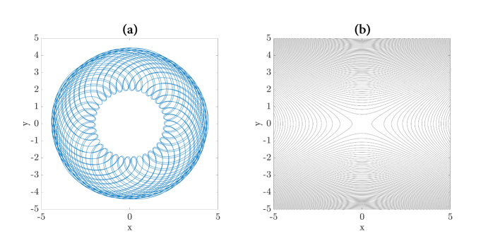
Figure 1: (a) A typical fluid particle trajectory generated by the linear unsteady velocity field (41) for the time interval $\left[t_{0},t_{1}\right]=\left[0,200\right]$ for the initial condition $\bm{x}_{0}=(2,0)$. This flow would appear as an unbounded vortex in any flow-visualization experiment involving dye or particles. (b) The instantaneous streamlines of the same velocity field, shown here for $t=0$, suggest a saddle point at the origin for all times (streamlines at other times look similar).

Mapped back into the original frame via the time-periodic transformation (30), the center-type trajectories become quasiperiodic. Figure 1(a) shows such a quasiperiodic particle trajectory and Fig. 1(b) instantaneous streamlines of the velocity field (6) with $\mathbf{h}(t)\equiv\mathbf{0}$, $a_{1}(t)=\mathrm{sin}4t$, $b_{1}(t)=\mathrm{cos}4t$, and $\omega=-1$ and $a_{k}=b_{k}\equiv 0$ for $k\geq 2$. These parameter values yield the velocity field

$$\mathbf{u}(\mathbf{x},t)=\left(\begin{array}[]{cc}\sin 4t&\cos 4t+\frac{1}{2}\\ \cos 4t-\frac{1}{2}&-\sin 4t\end{array}\right)\mathbf{x},$$ (41)

which satisfies $|\omega-C|>2$. This flow would, therefore, appear as an unbounded vortex in any flow visualization experiment involving dye or particles, yet its instantaneous streamlines suggest a saddle point at the origin for all times. Similarly, the Okubo–Weiss criterion incorrectly pronounces the entire plane hyperbolic for the flow (41) for all times. Indeed, formula (24) gives

$$OW\equiv 1-\frac{\omega^{2}}{4}=\frac{7}{16}>0.$$ (42)

Example 2.

By the general formula (6), a simple quadratic extension of the linear velocity field (28) is given by the universal Navier–Stokes solution

$$\mathbf{u}(\mathbf{x},t)=\left(\begin{array}[]{cc}\sin 4t&\cos 4t+2\\ \cos 4t-2&-\sin 4t\end{array}\right)\mathbf{x}+\alpha(t)\left(\begin{array}[]{c}x^{2}-y^{2}\\ -2xy\end{array}\right),$$ (43)

where we have chosen $a_{2}(t)\equiv\alpha(t)$ and $b_{2}(t)\equiv 0$ in the quadratic terms of (6), and set $\mathbf{h}(t)$, $a_{k}(t)$ and $b_{k}$ for $k>2$, as in Example 1. Setting $\alpha(t)\equiv-0.1$ for simplicity, we find that the instantaneous streamlines now suggest a bounded spinning vortex enclosed by connections between two stagnation points. The Okubo–Weiss criterion also suggests a coherent vortex surrounding the origin at all times, as $OW<0$ holds on a yellow domain shown containing the origin, as shown in Fig. 2(a). In reality, however, the origin is a saddle-type Lagrangian trajectory with transversely intersecting stable and unstable manifolds.

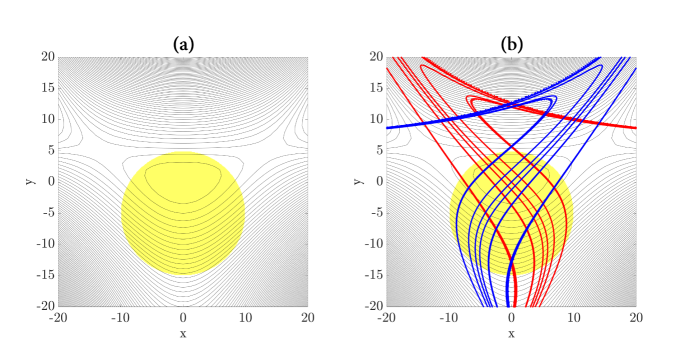
Figure 2: (a) Instantaneous streamlines and Okubo–Weiss elliptic region (yellow) for the universal Navier–Stokes solution (43) with $\alpha(t)\equiv-0.1$ at time $t=0$. Other time slices are similar. (b) Stable (blue) and unstable (red) manifolds of the fixed point of the Poincaré map (based at $t=0$ with period $T=\frac{\pi}{2}$) for the Lagrangian particle motions under the same velocity field, superimposed on the structures shown in (a).

Shown in Fig. 2(b) for the Poincaré map of the flow, the resulting homoclinic tangle creates intense chaotic mixing. This mixing process rapidly removes all but a measure zero set of initial conditions from the Okubo–Weiss vortical region. Therefore, the Navier–Stokes solution (43) with $\alpha(t)\equiv-0.1$ provides a clear false positive for coherent material vortex detection based on streamlines and on the Okubo–Weiss criterion.

Example 3.

Building on the discussion of the stability of the $x=0$ fixed point of equation (29), we now consider another specific Navier–Stokes velocity field of the form

$$\mathbf{u}(\mathbf{x},t)=\left(\begin{array}[]{cc}\sin 4t&\cos 4t+\frac{1}{2}\\ \cos 4t-\frac{1}{2}&-\sin 4t\end{array}\right)\mathbf{x}+\alpha(t)\left(\begin{array}[]{c}x^{2}-y^{2}\\ -2xy\end{array}\right),$$ (44)

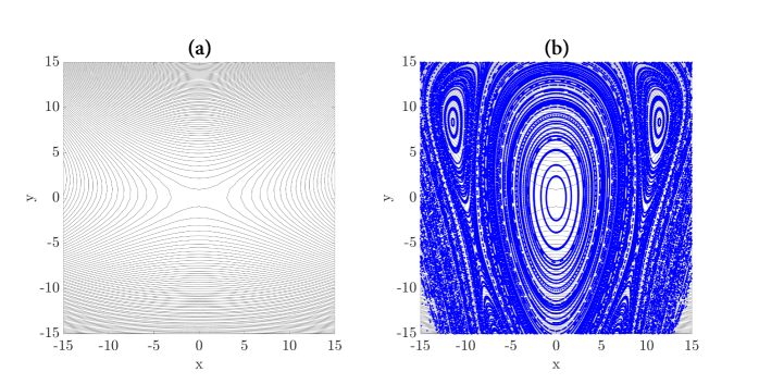
Figure 3: (a) Instantaneous streamlines for the universal Navier–Stokes solution (44) with $\alpha(t)\equiv-0.015$ at time $t=0$. Other time slices are similar. (b) KAM curves (blue) of the same velocity field, superimposed on the streamlines shown in (a).

from the universal solution family (6). In the notation used for equation (29), we now have $\omega=-1$ and $C=4,$ which gives $|C-\omega|>2$. Therefore, as discussed in Example 1, the origin of (44) is a center-type fixed point under linearization for the Lagrangian particle motion. At the same time, both the instantaneous streamlines in Fig. 3(a) and the Okubo–Weiss criterion suggest saddle-type (hyperbolic) behavior for the linearized flow, given that $OW>0$ holds on the whole plane. By the Kolmogorov–Arnold–Moser (KAM) theorem Arnold (1989), however, setting the small parameter $\alpha(t)\equiv-0.015$ in (44) is expected to preserve the elliptic (vortical) nature of the Lagrangian particle motion in the quadratic velocity field (44). Indeed, most quasiperiodic motions of the linearized system survive with the exception of resonance islands, as indicated by the KAM curves shown in blue in Fig. 3(b). Therefore, the Navier–Stokes solution (44) with $\alpha(t)\equiv-0.015$ provides a false negative for coherent material vortex detection based on streamlines or the Okubo–Weiss criterion. Note that the KAM curves shown in some of the examples in this section were obtained by launching fluid particles from a uniformly spaced grid over the domain shown, advecting them over the time span $\left[0\ 2\pi\right]$, and plotting the advected positions of the fluid particles at each time step.

Example 4.

By the general formula (6), a cubic extension of (28) is given by the universal Navier–Stokes solution

$$\mathbf{u}(\mathbf{x},t)=\left(\begin{array}[]{cc}\sin 4t&\cos 4t+2\\ \cos 4t-2&-\sin 4t\end{array}\right)\mathbf{x}+\alpha(t)\left(\begin{array}[]{c}x\left(x^{2}-3y^{2}\right)\\ -y\left(3x^{2}-y^{2}\right)\end{array}\right),$$ (45)

where we have chosen $a_{2}(t)\equiv 0$, $b_{2}(t)\equiv 0$, $a_{3}(t)\equiv\alpha(t)$ and $b_{3}(t)\equiv 0$ in the quadratic and cubic terms of (6), respectively, and set $\mathbf{h}(t)$, $\omega$, $a_{k}(t)$ and $b_{k}(t)$ for $k>3$ as in Example 2. We also set $\alpha(t)\equiv 0.005$. The instantaneous streamlines, shown in Fig. 4(a) for $t=0$, suggest a bounded spinning vortex around the origin surrounded by two saddle-type structures. Similarly, the Okubo–Weiss criterion, visualized by the yellow domain ($OW<0$) in Fig. 4(a), suggests a coherent vortex surrounding the origin at all times.

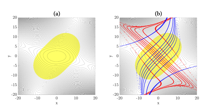
Figure 4: (a) Instantaneous streamlines and Okubo–Weiss elliptic region (yellow) for the universal Navier–Stokes solution (45) with $\alpha(t)\equiv 0.005$ at time $t=0$. Other time slices are similar. (b) Stable (blue) and unstable (red) manifolds of the fixed point of the Poincaré map (based at $t=0$ with period $T=\frac{\pi}{2}$) for the Lagrangian particle motions under the same velocity field, superimposed on the structures shown in (a).

The actual Lagrangian dynamics, however, is again strikingly different: Shown in Fig. 4(b), the Poincaré map of the flow shows that the origin is a saddle-type Lagrangian trajectory with transversely intersecting stable (blue) and unstable (red) manifolds, which lead to chaotic mixing near the origin. Therefore, the Navier–Stokes solution (45) with $\alpha(t)\equiv 0.005$ provides, similarly to Example 2, a false positive for coherent material vortex detection based on streamlines and on the Okubo–Weiss criterion.

Example 5.

We now consider another universal Navier–Stokes solution of the form

$$\mathbf{u}(\mathbf{x},t)=\left(\begin{array}[]{cc}\sin 4t&\cos 4t+\frac{1}{2}\\ \cos 4t-\frac{1}{2}&-\sin 4t\end{array}\right)\mathbf{x}+\alpha(t)\left(\begin{array}[]{c}x\left(x^{2}-3y^{2}\right)\\ -y\left(3x^{2}-y^{2}\right)\end{array}\right),$$ (46)

where we have chosen $a_{2}(t)\equiv 0$, $b_{2}(t)\equiv 0$, $a_{3}(t)\equiv\alpha(t)$ and $b_{3}(t)\equiv 0$ in the quadratic and cubic terms of (6), respectively, and selected $\mathbf{h}(t)$, $\omega$, $a_{k}(t)$ and $b_{k}(t)$, for $k=2$ and $k>3$ as in Example 1. As discussed in Example 3, for the choice of a small parameter $\alpha(t)\equiv 0.005$, we expect, by the KAM theorem Arnold (1989), that most quasiperiodic motions linearized system survive around the origin. Contrary to this, the instantaneous streamline picture, shown in Fig. 5(a) for $t=0$, suggests a stagnation point at the origin. The Okubo–Weiss criterion, visualized by the yellow domains ($OW<0$) in Fig. 5(a), predicts two coherent vortices away from the origin. Fig. 5(b) shows in blue KAM curves of the velocity field (46), revealing a bounded material coherent vortex around the origin. The rest of the particles, which are not captured by the material vortex, escape to infinity. Hence the Okubo–Weiss criterion provides one false negative and two false positives for vortex identification in the velocity field (46).

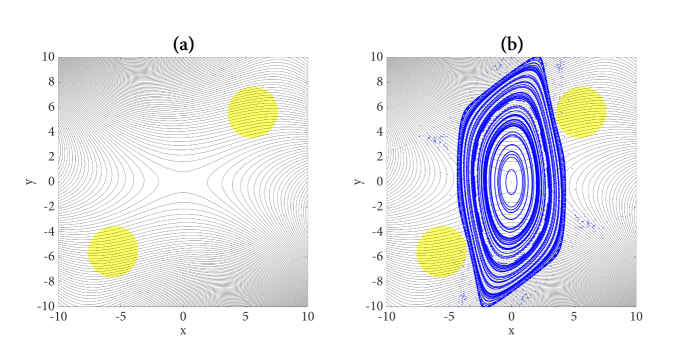
Figure 5: (a) Instantaneous streamlines and Okubo–Weiss elliptic region (yellow) for the universal Navier–Stokes solution (46) with $\alpha(t)\equiv 0.005$ at time $t=0$. Other time slices are similar. (b) KAM curves (blue) of the same velocity field.

Example 6.

A further extension of the velocity field (46) is given by the universal Navier–Stokes solution

$$\mathbf{u}(\mathbf{x},t)=\left(\begin{array}[]{cc}\sin 10t&\cos 10t+2\\ \cos 10t-2&-\mathrm{sin}10t\end{array}\right)\mathbf{x}+\alpha(t)\left(\begin{array}[]{c}x\left(x^{2}-3y^{2}\right)\\ -y\left(3x^{2}-y^{2}\right)\end{array}\right),$$ (47)

where we have chosen $a_{2}(t)\equiv 0$, $b_{2}(t)\equiv 0$, $a_{3}(t)\equiv\alpha(t)$ and $b_{3}(t)\equiv 0$ in the quadratic and cubic terms of (6), respectively, and set $\mathbf{h}(t)$, $\alpha(t)$, $\omega$, $a_{k}(t)$ and $b_{k}(t)$ for $k>3$ as in Example 4. This solution is a nonlinear extension of the general linear velocity field (29), with $\omega=-2$ and $C=10$. Therefore, as for the solution (44), $|C-\omega|>2$. Hence the origin of (47) is a center-type fixed point of the linearized system. By the KAM theorem Arnold (1989), adding a nonlinear term multiplied by the small parameter $\alpha(t)\equiv 0.005$ in (47), the Lagrangian particle motion in the cubic velocity field (47) is expected to remain elliptical (vortical) around the origin. The instantaneous streamlines of (47), shown in Fig. 6(a) for $t=0$, suggest a coherent vortex around the origin. The Okubo–Weiss criterion, visualized in Fig. 6(a) for the initial time $t=0$ by the yellow domain ($OW>0$), also suggests a coherent vortex near the origin.

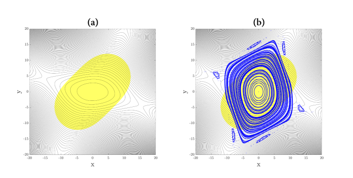
Figure 6: (a) Instantaneous streamlines and Okubo–Weiss elliptic region (yellow) for the universal Navier–Stokes solution (47) with $\alpha(t)\equiv 0.005$ at time $t=0$. Other time slices are similar. (b) KAM curves (blue) of the same velocity field.

Shown in blue in Fig. 6(b) are KAM curves of the flow, revealing indeed a bounded coherent vortex around the origin. The rest of the particles, which are not captured by the material vortices around the origin, escape to infinity. Hence for the solution (47), both the Okubo–Weiss criterion and the instantaneous streamlines correctly predict the presence of a coherent vortex around the origin. At the same time, they fail to predict the correct shape of the vortex, and completely miss six smaller vortices surrounding the large vortex in Fig. 6(b).

V Conclusions

We have derived an explicit form for all spatially polynomial, universal, planar Navier–Stokes flows up to arbitrary order. We then used examples of such solutions to test the ability of the instantaneous streamlines and of the Okubo–Weiss criterion, the 2D version of the $Q$-criterion, to detect coherent material vortices and stretching regions in unsteady flows.

Specifically, using the main result of this paper, we have derived two chaotically mixing Navier–Stokes flows whose analysis via instantaneous streamlines and by the Okubo–Weiss criterion suggests a lack of stretching due to the presence of a coherent vortex. Likewise, we have constructed two exact Navier–Stokes flows that have a bounded coherent Lagrangian vortex around the origin despite the hyperbolic flow structure suggested by instantaneous streamlines and the Okubo–Weiss criterion. Finally, we have constructed a Navier–Stokes solution whose trajectories form a coherent vortex near the origin. While the Okubo–Weiss criterion and the instantaneous streamlines do signal a nearby vortex in this example, they fail to render the correct shape of the vortex and miss additional smaller vortices in its neighborhood.

Using the 2D unsteady solutions, we have given an explicit family of unsteady polynomial solutions to the 3D Navier–Stokes equation. The first two coordinates of these 3D velocity fields agree with our planar polynomial solutions, while their third coordinate is simply a uniform, constant velocity component. When applied to these extended unsteady solutions, the $Q$-, $\Delta$-, $\lambda_{2}$- and $\lambda_{ci}$-criteria give the same incorrect flow classification results as the Okubo–Weiss criterion does in our two-dimensional examples.

The exact solutions derived in this paper can be used as basic unsteady benchmarks for coherent structure detection criteria and numerical schemes. They also provide a wealth of bounded, dynamically consistent flow patterns away from boundaries. For instance, the specific two-dimensional velocity field examples we have derived can be viewed as models of coherent structures, such as eddies and fronts, in oceanic flows away from the coastlines.