Bayesian posterior repartitioning for nested sampling

Abstract

Priors in Bayesian analyses often encode informative domain knowledge that can be useful in making the inference process more efficient. Occasionally, however, priors may be unrepresentative of the parameter values for a given dataset, which can result in inefficient parameter space exploration, or even incorrect inferences, particularly for nested sampling (NS) algorithms. Simply broadening the prior in such cases may be inappropriate or impossible in some applications. Hence our previous solution to this problem, known as posterior repartitioning (PR), redefines the prior and likelihood while keeping their product fixed, so that the posterior inferences and evidence estimates remain unchanged, but the efficiency of the NS process is significantly increased. In its most practical form, PR raises the prior to some power $\beta$, which is introduced as an auxiliary variable that must be determined on a case-by-case basis, usually by lowering $\beta$ from unity according to some pre-defined ‘annealing schedule’ until the resulting inferences converge to a consistent solution. Here we present a very simple yet powerful alternative Bayesian approach, in which $\beta$ is instead treated as a hyperparameter that is inferred from the data alongside the original parameters of the problem, and then marginalised over to obtain the final inference. We show through numerical examples that this Bayesian PR (BPR) method provides a very robust, self-adapting and computationally efficient ‘hands-off’ solution to the problem of unrepresentative priors in Bayesian inference using NS. Moreover, unlike the original PR method, we show that even for representative priors BPR has a negligible computational overhead relative to standard nesting sampling, which suggests that it should be used as the default in all NS analyses.

, and

1 Introduction

In recent years, Monte Carlo sampling techniques have been widely used in Bayesian inference problems both for parameter estimation and model selection. Nested sampling (NS) (Skilling, 2006) is one such approach that can simultaneously produce samples from the posterior distribution and estimate the marginal likelihood (or evidence). The NS algorithm involves drawing samples from a pre-defined prior distribution, and then evaluating their corresponding likelihoods, which are dependent on some measurement (or forward) model and the observed data. In general, the observed data are fixed and the measurement model is defined by field experts, with little room for flexibility. In contrast, the prior that identifies the regions of interest in the parameter space is typically much more loosely determined and often defined using simple standard distributions, together occasionally with physical constraints on the parameters $\bm{\theta}$ of the problem under consideration.

As we discussed in Chen et al. (2018), the NS algorithm can become very inefficient, or even fail completely in extreme cases, if the likelihood for a given data set is concentrated far out in the wings of the assumed prior distribution. This problem can be particularly damaging in applications where one wishes to perform analyses on many thousands (or even millions) of different datasets, since those (typically few) datasets for which the prior is unrepresentative can absorb a large fraction of the computational resources.

The problem occurs because the NS algorithm begins by drawing a number of ‘live’ samples from the prior and at each subsequent iteration replaces the sample having the lowest likelihood with a sample again drawn from the prior but constrained to have a higher likelihood. Thus, as the iterations progress, the collection of ‘live points’ gradually migrates from the prior to regions of high likelihood. When the likelihood is concentrated very far out in the wings of the prior, this process can become very slow, even in the rare problems where one is able to draw each new sample from the constrained prior using standard methods (sometimes termed perfect nested sampling). In practical problems, the issue is yet more pronounced since algorithms such as MultiNest (Feroz et al., 2009) and PolyChord (Handley et al., 2015) use other methods that may require several likelihood evaluations before a new sample is accepted. Depending on the method used, an unrepresentative prior can thus result in a significant drop in sampling efficiency, thereby increasing still further the required number of likelihood evaluations.

In extreme cases, the migration of live points in the NS process can be very slow, since over many iterations the live points will typically all lie in a region over which the likelihood is very small and flat. Indeed, in some such cases, the log-likelihoods of the set of live points may be indistinguishable to machine precision, so the ‘lowest likelihood’ sample to be discarded will be chosen effectively at random and, in seeking a replacement sample that is drawn from the prior but having a larger likelihood, the algorithm is very unlikely to obtain a sample for which the likelihood value is genuinely larger to machine precision. These problems can result in the live point set migrating exceptionally slowly, or becoming essentially stuck, such that the algorithm (erroneously) terminates before reaching the main body of the likelihood and therefore fails to produce correct posterior samples or evidence estimates.

One may, of course, seek to improve the performance of NS in such cases by increasing the number of live points and/or adjusting the convergence criterion, so that many more NS iterations are performed, but there is no guarantee in any given problem that these measures will be sufficient to prevent premature convergence. Perhaps more useful is to ensure that there is a greater opportunity at each NS iteration of drawing candidate replacement points from regions of the parameter space where the likelihood is larger. This may be achieved in a variety of ways. In MultiNest, for example, one may reduce the efr parameter to enlarge the volume of the multi-ellipsoidal bound from which candidate replacement points are drawn. Alternatively, as in other NS implementations, one may draw candidate replacement points using either MCMC sampling (Feroz and Hobson, 2008) or slice-sampling (Handley et al., 2015) and increase the number of steps taken before a candidate point is chosen. All of these approaches may mitigate the problem to some degree in particular cases, but only at the cost of a simultaneous dramatic drop in sampling efficiency caused precisely by the changes made in obtaining candidate replacement points. Moreover, in more extreme cases, these measures may fail completely.

Aside from making changes to the implementation of the NS algorithm itself, one might consider simple solutions such as broadening the prior range in such cases, but this might not be appropriate or possible in real-world applications, for example when one wishes to assume a single standardised prior across the analysis of a large number of datasets for which the true values of the parameters of interest may vary.

In Chen et al. (2018), we therefore proposed a posterior repartitioning (PR) method that circumvents the above difficulties. The PR method exploits the intrinsic degeneracy between the ‘effective’ likelihood and prior in the formulation of Bayesian inference problems. This is especially relevant for NS since it differs from other sampling methods by making use of the likelihood $\mathcal{L}(\bm{\theta})$ and prior $\pi(\bm{\theta})$ separately in its exploration of the parameter space, in that samples are drawn from the prior $\pi(\bm{\theta})$ such that they satisfy $\mathcal{L}(\bm{\theta})>L_{\ast}$, where $L_{\ast}$ is some predefined likelihood constraint. By contrast, Markov chain Monte Carlo (MCMC) sampling methods or genetic algorithm variants are typically blind to this separation, and deal solely in terms of the product $\mathcal{L}(\bm{\theta})\pi(\bm{\theta})$, which is proportional to the posterior $\mathcal{P}(\bm{\theta})$. This difference provides an opportunity in the case of NS to ‘repartition’ the product $\mathcal{L}(\bm{\theta})\pi(\bm{\theta})$ by defining a new effective likelihood $\tilde{\mathcal{L}}(\bm{\theta})$ and prior $\tilde{\mathit{\pi}}(\bm{\theta})$ (which is typically ‘broader’ than the original prior), subject to the condition $\tilde{\mathcal{L}}(\bm{\theta})\tilde{\mathit{\pi}}(\bm{\theta})=\mathcal{L}(\bm{\theta})\pi(\bm{\theta})$, so that the (unnormalised) posterior remains unchanged. Thus, in principle, the inferences obtained are unaffected by the use of the PR method, but, as we demonstrated in Chen et al. (2018), the approach can yield significant improvements in sampling efficiency and also helps to avoid the convergence problems that can occur in extreme examples of unrepresentative priors.

In general, the effective prior $\tilde{\mathit{\pi}}(\bm{\theta})$ can be any distribution that can be sampled straightforwardly, which in principle can be arbitrary (Alsing and Handley, 2021), but should at least be non-zero everywhere that the original prior is non-zero. In its most practical form, however, sometimes termed power posterior repartitioning (PPR), the effective prior $\tilde{\mathit{\pi}}(\bm{\theta})$ is proportional simply to the original prior $\pi(\bm{\theta})$ raised to some power $\beta$, which is introduced as an auxiliary variable. Although we demonstrated the effectiveness of this approach in Chen et al. (2018), one drawback of our original method is that the auxiliary variable must be determined on a case-by-case basis, which is typically achieved by lowering $\beta$ from unity, outside the execution of the NS algorithm, according to some pre-defined ‘annealing schedule’, until the resulting inferences from successive NS runs converge to a statistically consistent solution for values below some (positive) threshold $\beta\lesssim\beta_{\ast}$. This approach lacks elegance and the repeated NS runs required can be computationally demanding. Moreover, the final inference is unavoidably conditioned on the value $\beta_{\ast}$.

In this paper, we therefore present an alternative, Bayesian approach, in which $\beta$ is instead treated as a hyperparameter that is inferred from the data alongside the original parameters $\bm{\theta}$ of the problem, within a single execution of the NS algorithm. Although this approach is conceptually very simple, indeed almost trivial, the resulting Bayesian PR (BPR) method is considerably more powerful than our original PR technique in several respects. In particular, one obtains samples from the joint posterior on $(\bm{\theta},\beta)$, which may then be used straightforwardly in a number of ways. First, one may properly marginalise over $\beta$ in a Bayesian manner to obtain a final inference on $\bm{\theta}$, rather than conditioning on a single value of $\beta$ as in the original PR approach. Moreover, this allows BPR to accommodate likelihood functions consisting of a number of spatially separated modes that are located asymmetrically with respect to the prior, and are therefore characterised by different ranges of $\beta$ values; this is not possible using the original PR method. Second, one may instead marginalise over $\bm{\theta}$ to determine the 1-dimensional marginal distribution of $\beta$ (an ‘effective’ posterior that will be introduced in later sections), which we will show is very useful in diagnosing both the existence and severity of an unrepresentative prior for a given dataset, and hence for identifying ‘outlier’ datasets and in refining the inference problem for future analyses. Finally, since the sampling of the joint posterior on $(\bm{\theta},\beta)$ is performed within a single NS run, BPR is much less computationally demanding than the original PR method, which requires a separate NS run for each value of $\beta$ in its annealing schedule. Indeed, since the overhead of introducing just a single additional hyperparameter $\beta$ to be sampled is negligible for most practical problems, BPR is typically no more computationally demanding than a standard NS analysis (i.e., equivalent to setting $\beta=1$), but automatically safeguards against potentially inefficient parameter space exploration, or even incorrect inferences, which may occur in the presence of unrepresentative priors. This suggests that BPR should, in fact, be used as the default approach in all NS analyses.

It is worth noting, however, that one may encounter even more extreme problems than those discussed above, where the likelihood for some dataset(s) is concentrated outside an assumed prior having compact support. From a probabilistic point of view, the prior in these problems has zero probability in the region of the likelihood distribution. This case, which one might describe as an unsuitable prior, is not addressed by the BPR method, and is not considered here.

This paper is organised as follows. Section 2 briefly introduces the Bayesian inference and the NS algorithm. In Section 3, we present a simple analytical illustration of the effect of an unrepresentative prior on Monte Carlo sampling in general and NS in particular. Section 4 outlines the original PR method and then describes the proposed BPR scheme. Section 5 demonstrates performance of the BPR method in some numerical examples, and we present our conclusions in Section 6.

2 Bayesian inference using nested sampling

Bayesian inference (see e.g. MacKay 2003) provides a consistent framework for estimating unknown parameters $\bm{\theta}$ of some model by updating any prior knowledge of $\bm{\theta}$ using the observed data $\mathcal{D}$ and an assumed measurement process. The complete inference is embodied in the posterior distribution of $\bm{\theta}$, which can be expressed using Bayes’ theorem as:

$$\Pr(\bm{\theta}|\mathcal{D},\mathcal{M})=\frac{\Pr(\mathcal{D}|\bm{\theta},\mathcal{M})\Pr(\bm{\theta}|\mathcal{M})}{\Pr(\mathcal{D}|\mathcal{M})},$$ (1)

where $\mathcal{M}$ represents model (or hypothesis) assumption(s), and adopting a simplifying notation, $\Pr(\bm{\theta}|\mathcal{D},\mathcal{M})\equiv\mathcal{P}(\bm{\theta})$ is the posterior probability density, $\Pr(\mathcal{D}|\bm{\theta},\mathcal{M})\equiv\mathcal{L}(\bm{\theta})$ is the likelihood, $\Pr(\bm{\theta}|\mathcal{M})\equiv\mathit{\pi}(\bm{\theta})$ is the prior probability density on $\bm{\theta}$ and $\Pr(\mathcal{D}|\mathcal{M})\equiv\mathcal{Z}$ is called the evidence (or marginal likelihood). We then have the simplified expression:

$$\mathcal{P}(\bm{\theta})=\frac{\mathcal{L}(\bm{\theta})\mathit{\pi}(\bm{\theta})}{\mathcal{Z}},$$ (2)

in which the evidence is given by

$$\mathcal{Z}=\int_{\cal R}\mathcal{L}(\bm{\theta})\mathit{\pi}(\bm{\theta})d\bm{\theta},$$ (3)

where $\cal R$ represents the prior space of $\bm{\theta}$. The evidence $\mathcal{Z}$ is often used for model selection. It is the average of the likelihood over the prior, considering every possible choice of $\bm{\theta}$, and thus is not a function of the parameters $\bm{\theta}$. The constant $\mathcal{Z}$ is usually ignored in parameter estimation, since the posterior $\mathcal{P}(\bm{\theta})$ is proportional to the product of likelihood $\mathcal{L}(\bm{\theta})$ and prior $\mathit{\pi}(\bm{\theta})$.

Nested sampling (Skilling, 2006) explores the posterior distribution in a sequential manner using a fixed number of $N_{\rm live}$ ‘live samples’ of the parameters $\bm{\theta}$ at each iteration of the process. Pseudo-code of standard NS algorithm is described in Supplementary Materials. Among the various implementations of the NS algorithm (Chopin and Robert, 2007; Feroz et al., 2009; Brewer et al., 2011; Handley et al., 2015; Baldock et al., 2017; Higson et al., 2018; Buchner, 2019; Speagle, 2020; Buchner, 2021), two widely used packages are MultiNest (Feroz et al., 2009, 2013) and PolyChord (Handley et al., 2015). MultiNest draws the new sample at each iteration using rejection sampling from within a multi-ellipsoid bound approximation to the iso-likelihood surface defined by the discarded point; the bound is constructed from the live points present at that iteration. PolyChord draws the new sample at each iteration using a number of successive slice-sampling steps taken in random directions, which is particularly well suited to higher-dimensional problems. Please see Feroz et al. (2009) and Handley et al. (2015) for more details.

3 Analytical illustration of Monte Carlo sampling with an unrepresentative prior

We begin by considering a simple intuitive example that illustrates the effect of an unrepresentative prior on Monte Carlo sampling algorithms in general and on NS in particular. We consider the case where both the likelihood and prior distributions are one-dimensional Gaussians defined by $\mathcal{L}(\mathbf{\mathit{\theta}})=\mathcal{N}(\mathbf{\mathit{\theta}};0,1)$ and $\mathcal{\pi}(\mathbf{\mathit{\theta}})=\mathcal{N}(\mathbf{\mathit{\theta}};\mu_{\mathit{\pi}},1)$, respectively, where $\mu_{\mathit{\pi}}$ is the mean of prior and $\bm{\theta}$ is rewritten as $\mathbf{\mathit{\theta}}$ for the one dimensional example. In this case, the fractional prior volume $X$ (which ranges between $[0,1]$ for NS) occupied by the region for which the likelihood exceeds the level $\mathcal{L}=\lambda$ is given by

$$X(\lambda)=\int_{-|\mathbf{\mathit{\theta}}(\lambda)|}^{|\mathbf{\mathit{\theta}}(\lambda)|}\mathcal{\pi}(\mathbf{\mathit{\theta}})\,d\mathbf{\mathit{\theta}}=\frac{1}{2}\left[\texttt{erf}\left(\frac{|\mathbf{\mathit{\theta}}(\lambda)|-\mu_{\mathit{\pi}}}{\sqrt{2}}\right)-\texttt{erf}\left(-\frac{|\mathbf{\mathit{\theta}}(\lambda)|+\mu_{\mathit{\pi}}}{\sqrt{2}}\right)\right].$$ (4)

where erf is the error function and $\mathbf{\mathit{\theta}}(\lambda)=\pm\sqrt{-\log(2\pi)-2\log(\lambda)}$ is the value of random variable $\mathbf{\mathit{\theta}}$ where the likelihood value is $\lambda$. Also, the fractional evidence contained in the complement region where the likelihood is below the level $\mathcal{L}=\lambda$ is:

$$\mathcal{Z}(X=X(\lambda)) =\left(\int_{-\infty}^{\infty}-\int_{-|\mathbf{\mathit{\theta}}(\lambda)|}^{|\mathbf{\mathit{\theta}}(\lambda)|}\right)\mathcal{L}(\mathbf{\mathit{\theta}})\mathcal{\pi}(\mathbf{\mathit{\theta}})d\mathbf{\mathit{\theta}}$$

$$=\frac{1}{2\sqrt{\pi}}\exp\left(-\frac{\mu_{\mathit{\pi}}^{2}}{4}\right)\left[1-\frac{1}{2}\left\{\texttt{erf}\left(\frac{\mu_{\mathit{\pi}}}{2}+|\mathbf{\mathit{\theta}}(\lambda)|\right)-\texttt{erf}\left(\frac{\mu_{\mathit{\pi}}}{2}-|\mathbf{\mathit{\theta}}(\lambda)|\right)\right\}\right].$$ (5)

We consider three cases for which the mean $\mu_{\mathit{\pi}}$ of the Gaussian prior equal to $1$, $5$ and $15$, respectively. In the first case, the prior and likelihood are consistent, while the other two cases correspond to increasingly unrepresentative priors. Figure 1 shows (a) the behavior of the likelihood $\mathcal{L}$ and (b) the evidence $\mathcal{Z}$ as a function of the prior volume $X$, all on a logarithmic scale.

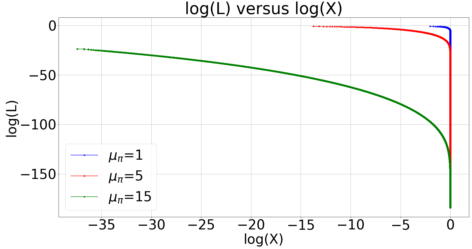
(a) $\text{log}\mathcal{L}$ against $\text{log}X$

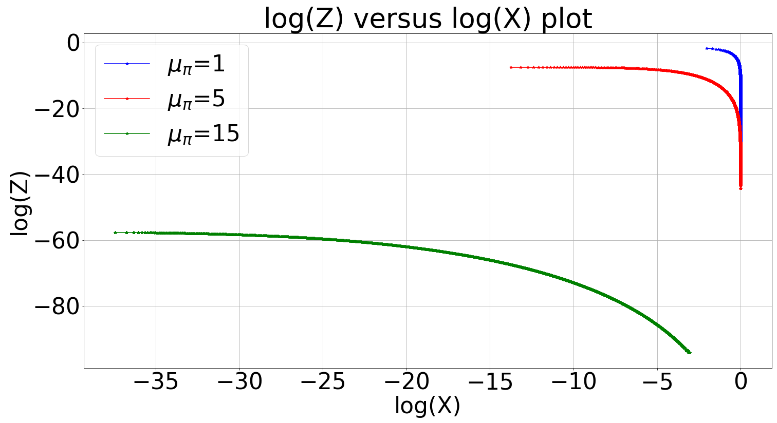
(b) $\text{log}\mathcal{Z}(X)$ against $\text{log}X$

Figure 1: Relationship between likelihood $\mathcal{L}(X)$ and evidence $\mathcal{Z}(X)$ (up to prior volume $X$) against the prior volume $X$ for the toy examples discussed in Sec. 3. The three curves in each figure represent the priors with mean $\mu_{\mathit{\pi}}$ equal to $1,5$ and $15$, respectively.

This figure shows that both $\mathcal{L}(X)\approx 0$ and $\mathcal{Z}(X)\approx 0$ (i.e., large negative values on a log-scale) in the case of an extreme unrepresentative with $\mu=15$ (green curve) for all values of $X$ except those very close to zero (or $\text{log}X\approx-\infty$). Also both $\log\mathcal{L}(X)$ and $\log\mathcal{Z}(X)$ increase more gradually with decreasing $\text{log}X$ as $\mu_{\mathit{\pi}}$ increases (and the prior becomes more unrepresentative). Therefore, for higher $\mu_{\mathit{\pi}}$ it becomes increasingly difficult for any Monte Carlo algorithm in general and NS in particular to proceed as the likelihood is almost zero over most of the prior space and increases very gradually as the NS algorithm proceeds to regions contained within iso-likelihood contours at progressively higher likelihood levels, resulting in premature convergence. This also explains the results shown in Figure 13(a) in the Supplementary Material, where standard NS experiences a sudden failure as the prior becomes increasingly unrepresentative.

4 Bayesian posterior repartitioning

In previous research, we first considered the possibility of improving the robustness and efficiency of NS by exploiting the intrinsic degeneracy between the ‘effective’ likelihood and prior in the formulation of Bayesian inference problems in Feroz et al. (2009), and then further developed the idea as the original PR method in Chen et al. (2018).

As mentioned in the Introduction, the central idea is to ‘repartition’ the product of the likelihood and prior, such that

$$\mathcal{L}(\bm{\theta})\mathit{\pi}(\bm{\theta})=\tilde{\mathcal{L}}(\bm{\theta})\tilde{\mathit{\pi}}(\bm{\theta}),$$ (6)

where $\tilde{\mathcal{L}}(\bm{\theta})$ and $\tilde{\mathit{\pi}}(\bm{\theta})$ are the newly-defined effective (or modified) likelihood and prior, respectively. As a result, the (unnormalised) posterior remains unchanged and hence, in principle, any parameter inferences are unaffected. Moreover, if $\tilde{\mathit{\pi}}(\bm{\theta})$ is normalised, then the evidence also remains unchanged. In general, $\tilde{\mathit{\pi}}(\bm{\theta})$ may be any distribution that can be straightforwardly sampled, and in principle can be arbitrary with sufficient effort (Alsing and Handley, 2021). For example, there is no requirement for the modified prior to be centred at the same parameter value as the original prior. One could, therefore, choose a modified prior that broadens and/or shifts the original one, or a modified prior that has a completely different form from the original. In this generalised setting, however, the modified prior should at least have the same support as the original prior.

In practice, rather than introducing a completely new prior distribution into the problem, a convenient choice (which we previously termed power PR) is simply to take $\tilde{\mathit{\pi}}(\bm{\theta})$ to be the original prior $\mathit{\pi}(\bm{\theta})$ raised to some (real) power $\beta$, and then renormalised to unit volume, such that

$$\tilde{\mathit{\pi}}(\bm{\theta}) = \frac{\mathit{\pi}(\bm{\theta})^{\mathit{\beta}}}{\mathcal{Z}_{\pi}(\beta)},$$ (7)

$$\tilde{\mathcal{L}}(\bm{\theta}) = \mathcal{L}(\bm{\theta})\mathit{\pi}(\bm{\theta})^{(1-\mathit{\beta})}\mathcal{Z}_{\pi}(\beta),$$ (8)

where $\mathit{\beta}\in[0,1]$ and $\mathcal{Z}_{\pi}(\beta)\equiv\int\mathit{\pi}(\bm{\theta})^{\mathit{\beta}}d\bm{\theta}$ is the normalisation constant of the modified prior. By altering the value of $\mathit{\beta}$, the modified prior varies across a range of distributions between the original prior ($\mathit{\beta}=1$) and the uniform distribution ($\mathit{\beta}=0$). This is illustrated in Figure 2 for five specific $\mathit{\beta}$ values in a one-dimensional case, where the original prior is a Gaussian with zero mean and standard deviation $\sigma_{\pi}=4$ and the normalisation depends on the assumed support $[-50,50]$ of the unknown parameter $\bm{\theta}$. The $\beta=0$ limit clearly yields a uniform modified prior $\tilde{\mathit{\pi}}(\bm{\theta})\sim\mathcal{U}({\cal R})$ over the allowed region ${\cal R}$ of the parameter space, which is an important special case in that it maximises the dispersion of the initial live point set across the prior space, but consequently can result in very inefficient sampling. It is worth noting that in the special case in which the original prior is uniform $\mathit{\pi}(\bm{\theta})\sim\mathcal{U}({\cal R})$, the power PR method is insensitive to the value of $\beta$ and defaults to standard NS. In principle, one may extend the upper limit on $\beta$ to exceed unity; this produces a new prior distribution that is sharper than the original, which may prove useful if the latter is over-dispersed. The power PR method does, however, have the limitation that one must be able to sample from the resulting modified prior and evaluate the normalising constant $\mathcal{Z}_{\pi}(\beta)$. If necessary, the latter may be estimated numerically, most efficiently in a separate NS run, for each value of $\beta$ used, but this may increase the computational costs significantly. Nonetheless, this issue may potentially be mitigated by pre-calculating $\mathcal{Z}_{\pi}(\beta)$ for a set of $\beta$ values and storing them in a look-up table, from which interpolation can be performed to approximate $\mathcal{Z}_{\pi}(\beta)$ for other $\beta$ values.

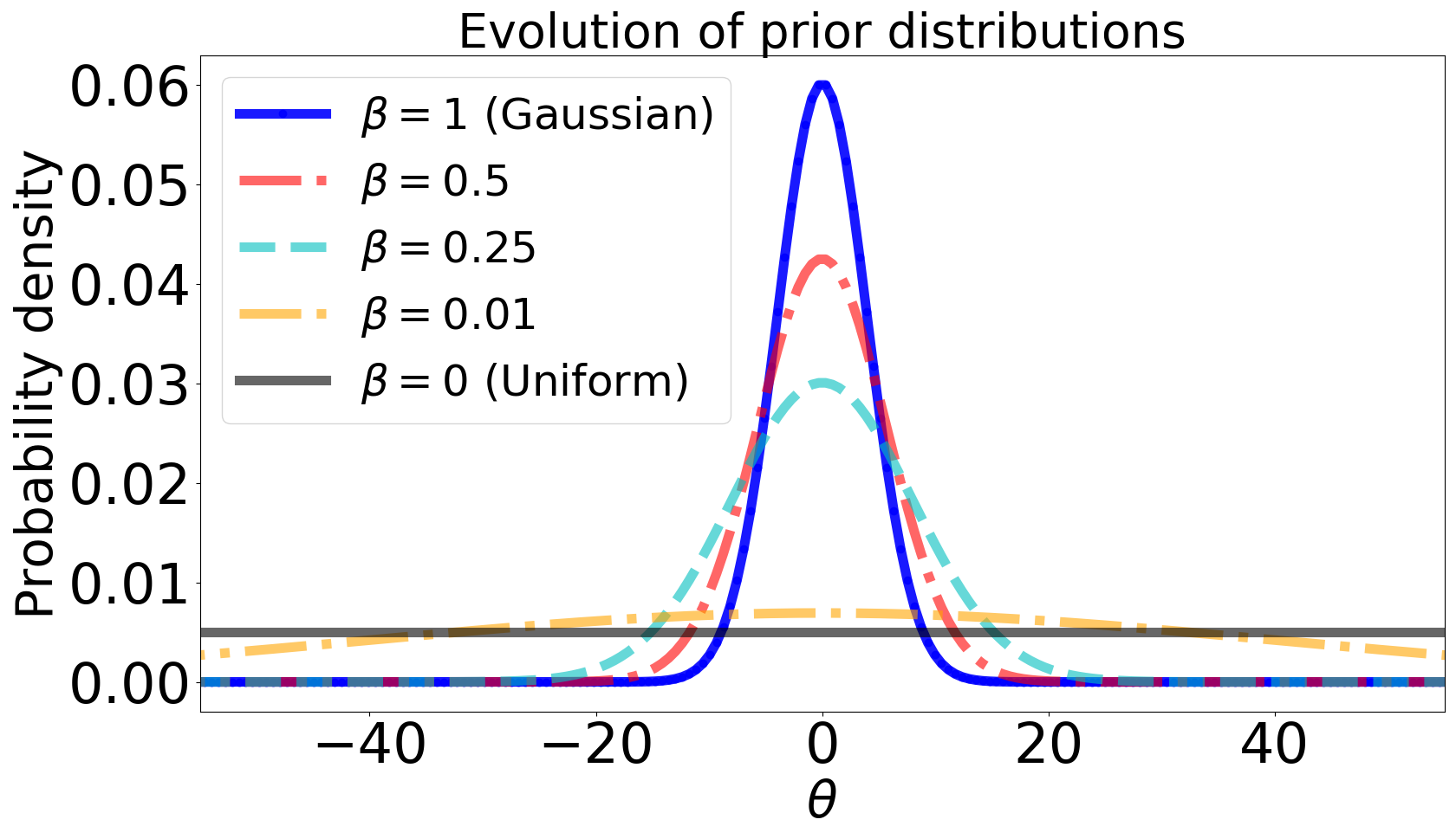
Figure 2: One-dimensional prior evolution for $\mathit{\beta}\in[0,1]$. The original prior is a Gaussian distribution with $\sigma_{\pi}=4$ (truncated in the range $[-50,50]$) when $\mathit{\beta}=1$ (solid blue curve), and is an uniform distribution when $\mathit{\beta}=0$ (solid black curve). The remaining three curves correspond to $\mathit{\beta}=0.5$ (dot-dashed red curve), $0.25$ (dashed light blue curve), $0.01$ (dot-dashed yellow curve), respectively.

A clear drawback of the original PR method, however, is that an appropriate value of the auxiliary variable $\beta$ must be determined on a case-by-case basis, and this can depend sensitively on the nature of the original prior and likelihood, as well as on the dimensionality of the problem under consideration. In Chen et al. (2018), we therefore suggested an approach in which $\beta$ is gradually lowered from unity (outside of the NS algorithm) according to some ‘annealing schedule’, until the resulting inferences from successive NS runs converge to a statistically consistent solution, which typically occurs for $\beta$ values below some (positive) threshold, $\beta\lesssim\beta_{\ast}$. Although we demonstrated in Chen et al. (2018) that this method is robust and effective, it has the disadvantages that there is a significant computational overhead associated with the multiple NS runs required and that the final inference of the parameters of interest $\bm{\theta}$ is conditioned on the adopted value $\beta=\beta_{\ast}$.

We therefore propose an alternative approach here, which we consider to be considerably more elegant, whereby $\beta$ is instead treated as a hyperparameter that is inferred in a fully Bayesian manner alongside the original parameters $\bm{\theta}$, within a single run of the NS algorithm. Although this approach is admittedly conceptually very simple, we view this as a virtue, in particular because the resulting Bayesian PR (BPR) method is considerably more powerful and flexible than the original PR technique in a number of important ways. The BPR method is based on defining the joint posterior

$$\tilde{\mathcal{P}}(\bm{\theta},\mathit{\beta})\propto\tilde{\mathcal{L}}(\bm{\theta},\mathit{\beta})\tilde{\mathit{\pi}}(\bm{\theta},\mathit{\beta})=\tilde{\mathcal{L}}(\bm{\theta},\mathit{\beta})\tilde{\mathit{\pi}}(\bm{\theta}|\mathit{\beta})\mathit{\pi}(\mathit{\beta}),$$ (9)

where $\mathit{\pi}(\mathit{\beta})$ denotes the assumed prior on the hyperparameter $\mathit{\beta}$, and $\tilde{\mathit{\pi}}(\bm{\theta}|\mathit{\beta})$ and $\tilde{\mathcal{L}}(\bm{\theta},\mathit{\beta})$ have precisely the forms (7) and (8), respectively. Since $\beta$ lies naturally in the range $[0,1]$, we define $\mathit{\pi}(\mathit{\beta})$ to be the uniform prior over this interval, although other choices may be accommodated if there is a strong motivation to adopt an alternative form in a particular problem. For example, if one wishes to extend the upper limit on $\beta$ to exceed unity to accommodate an over-dispersed original prior $\mathit{\pi}(\bm{\theta})$ on the parameters, a natural prior on $\mathit{\beta}$ is $\mathit{\pi}(\mathit{\beta})=e^{-\mathit{\beta}}$ in the range $[0,\infty]$, which is the maximum-entropy distribution for a non-negative quantity for which one knows only that its expectation value is unity. In any case, from the relations (6) and (2), one sees that (by construction)

$$\tilde{\mathcal{P}}(\bm{\theta},\mathit{\beta})\propto\mathcal{P}(\bm{\theta})\pi(\beta).$$ (10)

Moreover, the corresponding evidence is given by

$$\tilde{\mathcal{Z}} =\int\!\!\!\int\tilde{\mathcal{L}}(\bm{\theta},\mathit{\beta})\tilde{\mathit{\pi}}(\bm{\theta},\mathit{\beta})\,d\bm{\theta}\,d\beta$$ (11)

$$=\int\mathcal{L}(\bm{\theta})\mathit{\pi}(\bm{\theta})\,d\bm{\theta}\,\int\pi(\beta)\,d\beta=\mathcal{Z},$$ (12)

so that the proportionality in (10) can be replaced by an equality.

In principle, a single NS run thus provides samples from the full joint posterior distribution (10), which can be used straightforwardly to obtain inferences on the original parameters $\bm{\theta}$ in a properly Bayesian manner by marginalising over $\beta$, since

$$\tilde{\mathcal{P}}(\bm{\theta})=\int\tilde{\mathcal{P}}(\bm{\theta},\mathit{\beta})\,d\beta=\int{\mathcal{P}}(\bm{\theta})\mathit{\pi}(\mathit{\beta})\,d\beta={\mathcal{P}}(\bm{\theta}).$$ (13)

Hence, the overall computational burden is much reduced compared to the original PR method, since one does not require the latter’s multiple NS runs, namely one for each value of $\beta$ in its annealing schedule, or more if runs with the same value of $\beta$ (particularly for large $\beta$ values) are liable to exhibit significant variation in their results because of the failure of the NS algorithm, thereby complicating the process of determining convergence of results as the annealing schedule proceeds. Moreover, the final inference on the parameters $\bm{\theta}$ in BPR is not conditioned on a particular value of $\beta$. As we will show in examples in Section 5, marginalising over $\beta$ also allows BPR to accommodate likelihood functions consisting of multiple spatially separated modes that are located asymmetrically with respect to the prior, and which are therefore characterised by different ranges of $\beta$ values; this is not possible using the original PR method.

A further advantage of BPR is that one may instead choose to marginalise over the original parameters $\bm{\theta}$ to obtain the 1-D ‘effective’ posterior on $\beta$. This should in principle simply recover the prior on $\mathit{\beta}$, since

$$\tilde{\mathcal{P}}(\mathit{\beta})=\int\tilde{\mathcal{P}}(\bm{\theta},\mathit{\beta})\,d\bm{\theta}=\int{\mathcal{P}}(\bm{\theta})\mathit{\pi}(\mathit{\beta})\,d\bm{\theta}=\pi(\mathit{\beta}).$$ (14)

Thus, if the NS procedure has correctly sampled from the joint posterior distribution $\tilde{\mathcal{P}}(\bm{\theta},\mathit{\beta})$, one has neither gained nor lost anything by introducing the hyperparameter $\beta$, apart perhaps from a slight increase in the computational burden as a result of increasing by one the dimensionality of the space to be sampled.

In practice, however, the situation is more subtle. For illustration, let us consider the case where the original prior $\pi(\bm{\theta})=\tilde{\mathit{\pi}}(\bm{\theta},1)$ is extremely unrepresentative of the dataset under analysis, so that the original likelihood $\mathcal{L}(\bm{\theta})=\tilde{\mathcal{L}}(\bm{\theta},1)$ is concentrated very far into the wings of $\pi(\bm{\theta})$. In the limit $N_{\rm live}\to\infty$, the NS algorithm would nonetheless converge correctly, yielding samples from the posterior (10) and an estimate of the evidence (12). For finite $N_{\rm live}$, however, live points drawn from $\tilde{\mathit{\pi}}(\bm{\theta},\mathit{\beta})$ at any NS iteration will typically have very low likelihood $\tilde{\mathcal{L}}(\bm{\theta},\mathit{\beta})$ for values of $\beta$ above some limiting threshold $\beta\gtrsim\beta_{+}$ (which will depend on $N_{\rm live}$), since the chance of these points lying within the main body of the likelihood $\tilde{\mathcal{L}}(\bm{\theta},\mathit{\beta})$ is vanishingly small. Depending on the precise nature of the original prior $\pi(\bm{\theta})$ and likelihood $\mathcal{L}(\bm{\theta})$, a similar phenomenon may also occur for values of $\beta$ below some other limiting threshold $\beta\lesssim\beta_{-}$ (which will also depend on $N_{\rm live}$), since in this case the modified prior may have a support that far exceeds that of the likelihood.

Thus, in the presence of unrepresentative priors where the NS algorithm may become very inefficient or even fail, one may obtain samples that are drawn not from (10), but instead from some ‘effective’ posterior

$$\tilde{\mathcal{P}}_{\rm eff}(\bm{\theta},\mathit{\beta})\propto\mathcal{P}(\bm{\theta})\tilde{\mathcal{P}}(\beta),$$ (15)

where the (unnormalised) marginal posterior $\tilde{\mathcal{P}}(\beta)$ is non-zero only in some range $\sim[\beta_{-},\beta_{+}]$. The form of this marginal posterior, in particular its extent in $\beta$, will be determined by how the NS algorithm fails for particular (extreme) values of $\beta$, which is in turn dependent on the particular NS implementation used and the associated control parameters (including generic NS parameters such as $N_{\rm live}$), as well as the nature of the original prior $\pi(\bm{\theta})$ and likelihood $\mathcal{L}(\bm{\theta})$. One would, however, expect there to be a range of $\beta$ values for which the NS algorithm does not fail, and so $\tilde{\mathcal{P}}(\beta)$ should coincide with $\pi(\beta)$ in this range. Beyond these very general considerations, there is a paucity of further theoretical arguments from which to predict the form of $\tilde{\mathcal{P}}(\beta)$.

Nonetheless, by marginalising (15) over $\beta$ one still obtains the posterior $\mathcal{P}(\bm{\theta})$ on the original parameters. Conversely, marginalising over $\bm{\theta}$ one obtains $\tilde{\mathcal{P}}(\beta)$ (in practice as a histogram constructed from the equally weighted posterior samples) and may hence observe its form and determine the values $\beta_{-}$ and $\beta_{+}$. In particular, the value of $\beta_{+}$ is useful in diagnosing both the existence and severity of an unrepresentative prior for a given dataset, and thereby identifying the dataset as an ‘outlier’. Here we will take $\beta_{-}$ and $\beta_{+}$ simply as the smallest and largest $\beta$ values, respectively, in the set of equally weighted posterior samples. Alternatively, one could apply some percentile thresholds (e.g. 1% and 99%) to the $\beta$ marginal, but in practice this leads to very similar values of $\beta_{-}$ and $\beta_{+}$. In any case, observing the form of $\tilde{\mathcal{P}}(\beta)$ obtained in the BPR method provides a far more robust and computationally efficient approach to identifying the presence and severity of unrepresentative priors than determining and interpreting the value $\beta_{\ast}$ in the original PR method below which the inferences converge.

Finally, in the presence of unrepresentative priors, the NS process will not yield an estimate of the evidence (12), but rather the ‘effective’ evidence

$$\tilde{\mathcal{Z}}_{\rm eff}\approx\tilde{\mathcal{Z}}\int\tilde{\mathcal{P}}(\mathit{\beta})\,d\mathit{\beta}=\mathcal{Z}\int\tilde{\mathcal{P}}(\mathit{\beta})\,d\mathit{\beta}.$$ (16)

One may, however, estimate the required evidence $\mathcal{Z}$, provided one can evaluate the factor $\int\tilde{\mathcal{P}}(\mathit{\beta})\,d\mathit{\beta}$. Fortunately, from the discussion above, this may be achieved by first scaling the distribution $\tilde{\mathcal{P}}(\mathit{\beta})$, represented as a histogram of equally-weighted posterior samples, such that the bin containing the largest number of samples has the volume $\int_{\beta_{\rm l}}^{\beta_{\rm u}}\pi(\beta)\,d\beta$, where $\beta_{\rm l}$ and $\beta_{\rm u}$ are the lower and upper limits of the bin, respectively. The factor $\int\tilde{\mathcal{P}}(\mathit{\beta})\,d\mathit{\beta}$ may then be calculated by summing up the volumes of all the bins in the resulting scaled histogram. This summation is equivalent to the simplest form of numerical quadrature, namely the rectangle rule, which adopts a polynomial of degree zero (a constant function) to pass through points $\textstyle\left({(\beta_{\rm l}^{b}+\beta_{\rm u}^{b})/2},h(\beta_{\rm l}^{b}+\beta_{\rm u}^{b})/2\right)$, where $\beta_{\rm l}^{b}$ and $\beta_{\rm u}^{b}$ are the lower and upper limits of the $b$th bin, and $h(\cdot)$ indicates the height of the bin. In principle, one may estimate the error in the quadrature and propagate this through to $\tilde{\mathcal{Z}}_{\rm eff}$ using Eqn. (16), but we do not perform this here.

5 Numerical examples

We now illustrate the performance of the BPR method in some numerical examples. Since we extensively studied the behaviour of our original PR method in a wide range of problems in Chen et al. (2018), including comparisons with other sampling algorithms such as Markov Chain Monte Carlo (MCMC) and importance sampling, we focus here primarily on the performance of BPR in the canonical case where the likelihood and prior on the original variables $\bm{\theta}$ are both Gaussian (although very mismatched in some examples), and hence so too is the posterior. In particular, we begin by considering the univariate case, before moving on to a bivariate example for which we consider both circularly-symmetric and asymmetric priors, where the latter may have zero, positive or negative correlation coefficient, respectively. To demonstrate the method further, however, we also consider several 2-dimensional non-Gaussian likelihoods: multi-modal likelihoods consisting of an equal mixture of four identical but spatially separated Gaussians, and a unimodal Laplacian likelihood (the latter example is presented in the Supplementary Material). Finally, we investigate higher-dimensional unimodal Gaussian likelihood examples, up to 10 dimensions. In these further examples, we consider only circularly-symmetric Gaussian priors for the sake of brevity.

In all our numerical examples, we use the NS package MultiNest (Feroz et al., 2009), with algorithm parameter settings similar to those used in Chen et al. (2018) for the study of our original PR method. Specifically, we set the number of live points $N_{\rm live}=100$, the desired sampling efficiency parameter ${\tt efr}=0.8$, which equals the ratio of the remaining prior volume to the volume of the multi-ellipsoid bound enclosing the active point set at each NS iteration, and the convergence tolerance parameter ${\tt tol}=0.5$, which corresponds to acceptable uncertainty on the estimated log-evidence (please refer to Feroz et al. (2009) for more details).

5.1 Univariate Gaussian likelihood

We begin by considering a simple one-dimensional estimation problem, for which the data consist of $N$ independent measurements $M=\{m_{1},\cdots,m_{n},\cdots,m_{N}\}$ of an unknown parameter $\mathbf{\mathit{\theta}}$, such that

$$m_{n}=\mathbf{\mathit{\theta}}+\mathit{\xi},$$ (17)

where $\mathit{\xi}$ denotes Gaussian noise $\mathit{\xi}\sim\mathcal{N}(\mu_{\mathit{\xi}},\sigma_{\mathit{\xi}}^{2})$. The likelihood is thus given by

$$\mathcal{L}(\mathbf{\mathit{\theta}})=\prod_{n=1}^{N}\left\{\frac{1}{\sqrt{2\pi\sigma_{\mathit{\xi}}^{2}}}\exp\left[-\frac{(m_{n}-{\color[rgb]{0,0,0}(\mathbf{\mathit{\theta}}+\mu_{\mathit{\xi}})})^{2}}{2\sigma_{\mathit{\xi}}^{2}}\right]\right\},$$ (18)

which has a Gaussian form. In particular, we set $\mu_{\mathit{\xi}}=0$, $\sigma_{\mathit{\xi}}=1$ and the number of measurements as $N=20$, so that the likelihood is a Gaussian centred around the true value of $\theta$ with a standard deviation of $\sim 1/\sqrt{20}\approx 0.22$. The prior distribution $\mathit{\pi}(\mathbf{\mathit{\theta}})$ is also assumed to be Gaussian $\mathbf{\mathit{\theta}}\sim\mathcal{N}(\mu_{\mathit{\pi}},\sigma_{\mathit{\pi}}^{2})$, where we set $\mu_{\mathit{\pi}}=0$ and $\sigma_{\mathit{\pi}}=4$. Therefore one expects a priori that the true value of $\mathbf{\mathit{\theta}}$ will lie in the range $[-12,12]$ with greater than $99.5\%$ probability. Finally, we assume the prior distribution of the auxiliary factor $\mathit{\beta}$ to be the unit uniform distribution $\mathit{\beta}\sim\mathcal{U}[0,1]$.

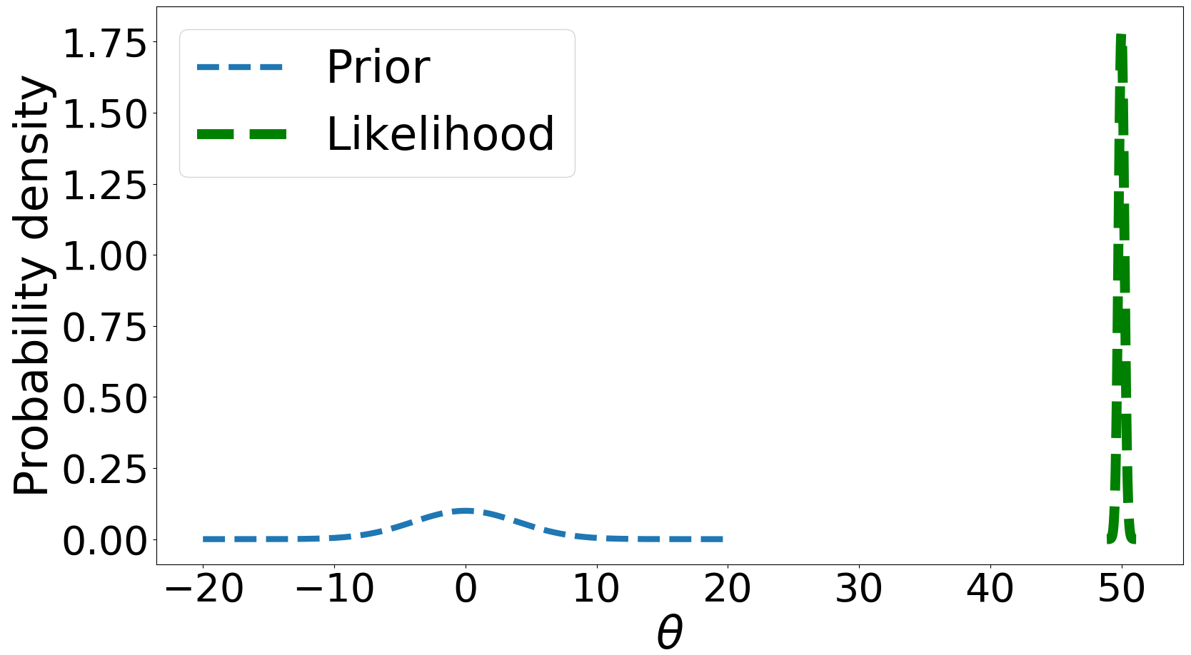
(a) unrepresentative prior, $\mathbf{\mathit{\theta}}_{\ast}=50$

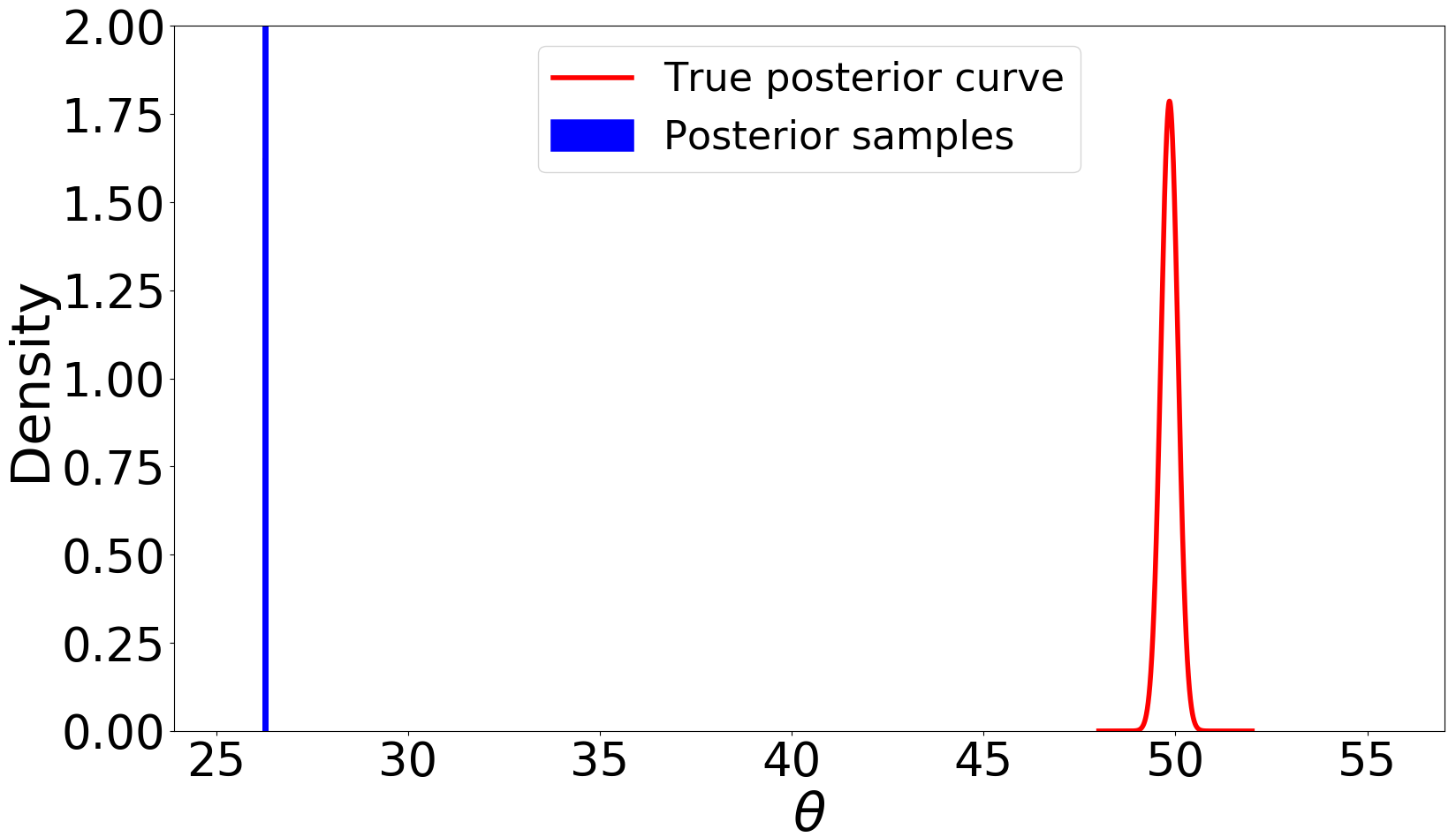
(b) estimated posterior by MultiNest, $\mathbf{\mathit{\theta}}_{\ast}=50$

Figure 3: Univariate Gaussian likelihood examples illustrating the unrepresentative case and the posterior samples obtained by standard MultiNest (blue histogram line). The light blue and green dashed curves denote the prior and the likelihood, respectively. The red curve represents the true Gaussian posterior.

We consider datasets corresponding to a series of true values $\mathbf{\mathit{\theta}}_{\ast}$ ranging between 5 and 50. Figure 3(a) shows the limiting example for $\mathbf{\mathit{\theta}}_{\ast}=50$, where the likelihood lies very far into the wings of the prior and may thus be considered unrepresentative for this data set. Figure 3(b) shows the posterior samples obtained using standard MultiNest without PR, together with the corresponding true Gaussian posterior. The behaviour in the limiting case is characteristic of a catastrophic failure mode of the NS algorithm in practice for extreme unrepresentative priors. This was first discussed in Chen et al. (2018) and here we take a step further to illustrate and discuss this behaviour in Figure 13 and Section 7.3 of the Supplementary Materials. Moreover, a discussion on failure probability of standard NS is also presented using the same univariate example as follows.

5.1.1 Failure probability of NS with univariate Gaussian likelihood

We calculate the failure probability of standard NS for the case where prior is a univariate Gaussian with mean $\mu_{\pi}$ and standard deviation $\sigma_{\pi}$. The likelihood is also a univariate Gaussian with mean $\mu_{\xi}$ and standard deviation $\sigma_{\xi}$ with $\mu_{\xi}>\mu_{\pi}$. We consider failure to be the case where there are no live points within $c\sigma_{\xi}$ of the likelihood mean $\mu_{\xi}$ after $I$ iterations. One could use $c=3$ here. The failure will very likely happen before $I$ iterations due to all live points being the same within machine precision, so we can take the failure probability estimate $p_{\rm fail}$ obtained here as its lower bound.

Before the first iteration, for the failure to happen, all $N_{\rm live}$ points have to be at values less than $(\mu_{\xi}-c\sigma_{\xi})$ which has probability:

$$p_{\rm fail,0}=\Phi(\mu_{\xi}-c\sigma_{\xi};\mu_{\pi},\sigma_{\pi})^{N_{\rm live}},$$ (19)

where $\Phi(x;\mu,\sigma)$ is the cumulative distribution function of Normal distribution and $p_{\rm fail,0}$ denotes the failure probability estimate at the $i=0$ iteration.

At each subsequent iteration $i$, if the remaining prior volume is $v_{\rm i}$ and the point with minimum likelihood value is at position $y_{i}$, then we have:

$$1-\Phi(y_{\rm i};\mu_{\pi},\sigma_{\pi})=v_{\rm i},$$ (20)

We can then calculate the probability of failure at iteration $i$, $p_{\rm fail,i}$ as:

$$p_{\rm fail,i} =\int_{0}^{1}\frac{P(v_{\rm i})\left(\Phi(\mu_{\xi}-c\sigma_{\xi};\mu_{\pi},\sigma_{\pi})-\Phi(y_{\rm i};\mu_{\pi},\sigma_{\pi})\right)}{v_{\rm i}}dv_{\rm i},$$ (21)

$$=\int_{0}^{1}\frac{P(v_{\rm i})\left(\Phi(\mu_{\xi}-c\sigma_{\xi};\mu_{\pi},\sigma_{\pi})-1+v_{\rm i}\right)}{v_{\rm i}}dv_{\rm i},$$

where the integral is over the distribution $P(v_{\rm i})$ of remaining prior volume $v_{\rm i}$ at iteration $i$ which itself equals to $v_{\rm i}=\prod_{\rm j=1}^{\rm i}t_{\rm j}$, where $P(t)=N_{\rm live}t^{N_{\rm live}-1}$ (Feroz et al., 2009) i.e. the distribution of the maximum of $N_{\rm live}$ uniformly distributed random variables and therefore $v_{\rm i}$ is the product of beta distributed random variables. It isn’t possible to get an analytical solution for the integral given in Eqn. 21. However, we can get an approximation by assuming $v_{\rm i}\approx\mathop{\mathbb{E}}[v_{\rm i}]$, where $\mathop{\mathbb{E}}[v_{\rm i}]=\exp(-i/N_{\rm live})$ (Feroz et al., 2009). Using this approximation in Eqn. 21 we get:

$$p_{\rm fail,i}\approx\frac{\Phi(\mu_{\xi}-c\sigma_{\xi};\mu_{\pi},\sigma_{\pi})-1+\mathop{\mathbb{E}}[v_{\rm i}]}{\mathop{\mathbb{E}}[v_{\rm i}]}.$$ (22)

We can now approximate the total failure probability $p_{\rm fail}$ as:

$$p_{\rm fail} \approx p_{\rm fail,0}\prod_{\rm i=1}^{\rm I}p_{\rm fail,i}$$ (23)

$$=\Phi(\mu_{\xi}-c\sigma_{\xi};\mu_{\pi},\sigma_{\pi})^{N_{\rm live}}\prod_{\rm i=1}^{\rm I}\frac{\Phi(\mu_{\xi}-c\sigma_{\xi};\mu_{\pi},\sigma_{\pi})-1+\mathop{\mathbb{E}}[v_{\rm i}]}{\mathop{\mathbb{E}}[v_{\rm i}]}.$$

We can use $p_{\rm fail}$ given above to explain the failure of standard NS in the univariate example discussed in this Section, i.e., $c=3,I=100,N_{\rm live}=100,\mu_{\pi}=0,\sigma_{\pi}=4,\sigma_{\xi}=0.22$. We can now calculate the failure probability $p_{\rm fail}$ for different values of $\mu_{\xi}$ (which is equal to $\theta_{*}$ in Figure 5). As shown in Figure 4, the failure probability increases rapidly for $\mu_{\xi}>10$ and therefore, we would expect $\beta<1$ for $\mu_{\xi}>10$ with BPR which is indeed what we see in Figure 5.

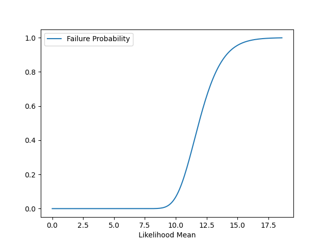
Figure 4: Failure probability of standard NS for the univariate Gaussian example as a function of mean of the likelihood distribution $\mu_{\xi}$ (which is equal to $\theta_{*}$ in the rest of this section).

The above illustrated issue of NS may be straightforwardly addressed by applying the BPR method. Figure 5 shows the resulting MultiNest (with BPR) joint posterior on $(\theta,\beta)$ and its marginals for a selection of true values $\theta_{\ast}$ in the range $[5,50]$ (the $\mathbf{\mathit{\theta}}_{\ast}=50$ case is plotted in brown). One sees that the joint posterior is precisely of the form expected in Eqn. (15), in that it is the product of two independent distributions on $\theta$ and $\beta$, respectively. One also observes the evolution of the marginal distribution on $\mathit{\beta}$. For each value of $\theta_{\ast}$, this is consistent with a top-hat distribution in the range $[0,\beta_{+}]$, where $\beta_{+}$ gradually decreases as $\theta_{\ast}$ increases. For $\theta_{\ast}\lesssim 10$, one sees that $\beta_{+}\approx 1$, so one recovers the original uniform prior distribution $\mathit{\beta}\sim\mathcal{U}[0,1]$, indicating that the original prior $\pi(\theta)$ is representative for these data sets. For $\theta_{*}\gtrsim 10$, however, the value of $\beta_{+}$ gradually decreases from unity as $\theta_{\ast}$ increases, which indicates that the original prior is increasingly unrepresentative for these data sets.

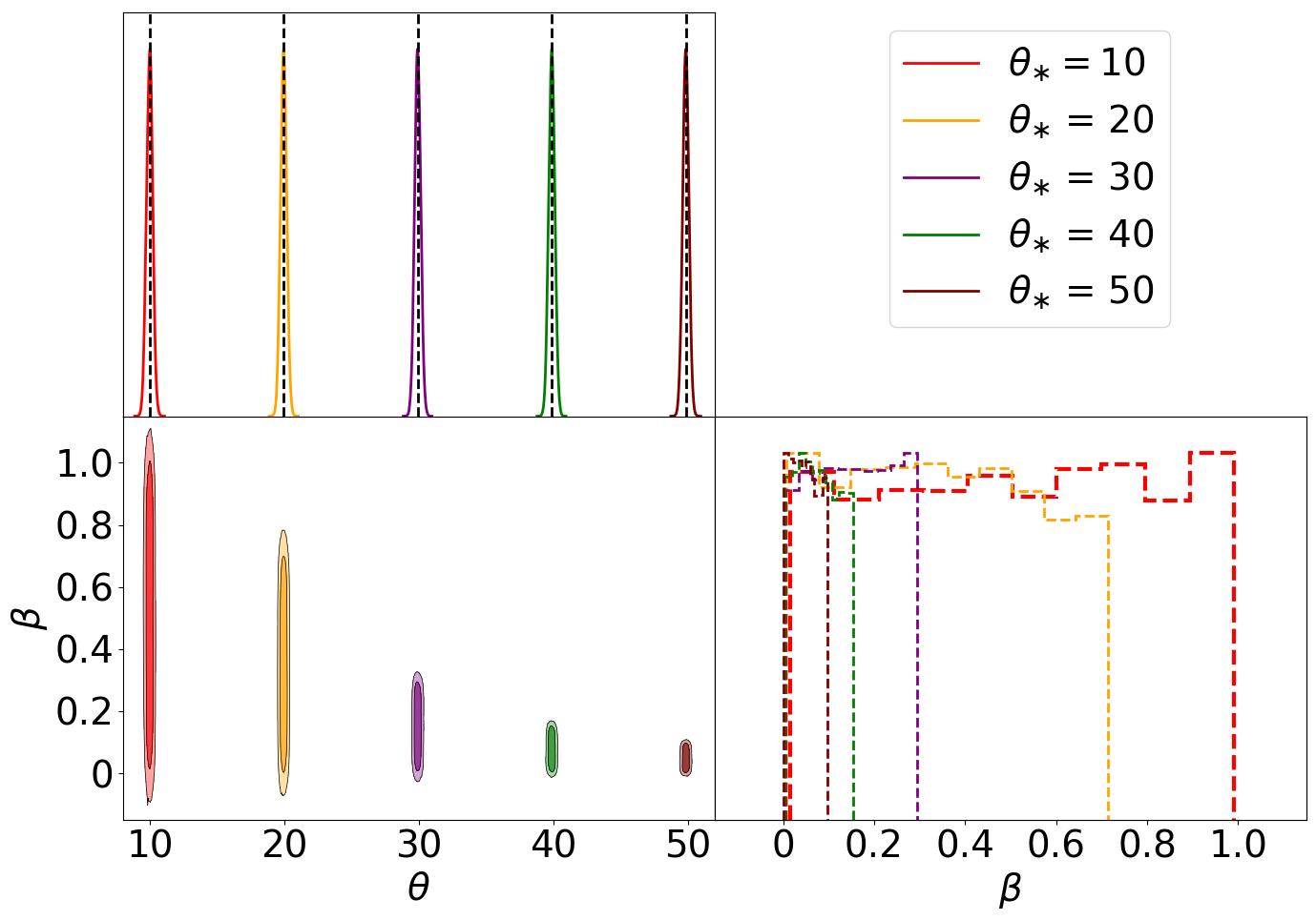
Figure 5: A ‘corner plot’ showing the joint posterior distribution on $(\theta,\beta)$ obtained by MultiNest using BPR, together with its marginals, for the univariate Gaussian likelihood example with a range of true values $\theta_{\ast}$. The vertical dashed black lines in the top left panel indicate the mean of the true Gaussian posterior in each case.

Turning to the marginals on $\mathbf{\mathit{\theta}}$ in Figure 5, one sees that they are correctly centred on the mean of the corresponding true Gaussian posterior for every value of $\mathbf{\mathit{\theta}}_{\ast}$. Moreover, the widths of the marginals on $\mathbf{\mathit{\theta}}$ are equal for each value of $\mathbf{\mathit{\theta}}_{\ast}$ and consistent with the width of the true Gaussian posterior, hence showing that BPR yields the correct inferences on $\mathbf{\mathit{\theta}}$, independent of the value of $\mathbf{\mathit{\theta}}_{\ast}$, in a fully automated manner, without any need for tuning. Quantitative results on both the parameter estimation accuracy on $\mathbf{\mathit{\theta}}$ and the evidence calculation are given in the Supplementary Material Section 7.3.

5.2 Bivariate Gaussian likelihood

We now move to a bivariate example, for which we consider both circularly-symmetric and asymmetric priors, where the latter may have zero, positive or negative correlation coefficient, respectively. In particular, consider a vectorised version of Eqn. (17) from the univariate Gaussian likelihood example, with some $K=2$ dimensional parameter vector $\bm{\theta}=(\mathbf{\mathit{\theta}}_{1},\mathbf{\mathit{\theta}}_{2})^{\top}$, such that

$$\mathbf{m}_{n}=\bm{\theta}+\bm{\xi},$$ (24)

where $\mathbf{m}=(m_{1},m_{2})^{\top}$, and $\bm{\xi}=(\mathit{\xi}_{1},\mathit{\xi}_{2})^{\top}$ denotes the two dimensional Gaussian noise $\bm{\xi}\sim\mathcal{N}(\bm{\mathit{\mu}}_{\bm{\xi}},\bm{\Sigma}_{\bm{\xi}})$ with mean $\bm{\mathit{\mu}}_{\bm{\xi}}$ and covariance $\bm{\Sigma}_{\bm{\xi}}$. The prior distribution is also Gaussian, $\bm{\theta}\sim\mathcal{N}(\bm{\mathit{\mu}}_{\mathbf{\mathit{\theta}}},\bm{\Sigma}_{\mathbf{\mathit{\theta}}})$. We assume unbiased measurements and priors centered on the origin, such that $\bm{\mathit{\mu}}_{\bm{\xi}}=(0,0)^{\top}=\bm{\mathit{\mu}}_{\mathbf{\mathit{\theta}}}$, and parameterise the noise and prior covariances matrices by

$$\bm{\Sigma}_{\bm{\xi}}=\begin{bmatrix}\sigma_{\mathit{\xi}_{1}}^{2}&\rho_{\mathit{\xi}}\sigma_{\mathit{\xi}_{1}}\sigma_{\mathit{\xi}_{2}}\\ \rho_{\mathit{\xi}}\sigma_{\mathit{\xi}_{2}}\sigma_{\mathit{\xi}_{1}}&\sigma_{\mathit{\xi}_{2}}^{2}\end{bmatrix},$$

$$\qquad\bm{\Sigma}_{\mathbf{\mathit{\theta}}}=\begin{bmatrix}\sigma_{\mathbf{\mathit{\theta}}_{1}}^{2}&\rho_{\mathbf{\mathit{\theta}}}\sigma_{\mathbf{\mathit{\theta}}_{1}}\sigma_{\mathbf{\mathit{\theta}}_{2}}\\ \rho_{\mathbf{\mathit{\theta}}}\sigma_{\mathbf{\mathit{\theta}}_{2}}\sigma_{\mathbf{\mathit{\theta}}_{1}}&\sigma_{\mathbf{\mathit{\theta}}_{2}}^{2}\end{bmatrix},$$

where $\rho_{\mathit{\xi}}$ and $\rho_{\mathbf{\mathit{\theta}}}$ are the standard correlation coefficients in each case.

In this example, we take the opposite approach to that used in the univariate example, in that we retain the same likelihood function for each case considered and instead vary the form of the assumed prior, although in all cases the prior is centred on the origin of the parameter space. In particular, we assume throughout the true value $\bm{\theta}_{\ast}=(40,40)^{\top}$, uncorrelated measurement noise with unit standard deviation, such that $\rho_{\mathit{\xi}}=0$ and $\sigma_{\mathit{\xi}_{1}}=\sigma_{\mathit{\xi}_{2}}=1$, and that the number of measurements is just $N=1$, as this yields a circularly-symmetric bivariate Gaussian likelihood distribution of unit standard deviation, which is convenient for our investigations. We present results only for the BPR method, since the standard NS approach fails in all the cases considered.

5.2.1 Uncorrelated priors

We begin by considering uncorrelated priors, for which $\rho_{\mathbf{\mathit{\theta}}}=0$. In particular, we consider the two circularly-symmetric cases where $\{\sigma_{\mathbf{\mathit{\theta}}_{1}}$, $\sigma_{\mathbf{\mathit{\theta}}_{2}}\}$ equals to $\{4,4\}$ and $\{2,2\}$, and the intermediate non-circularly-symmetric case $\{2,4\}$. These priors and the likelihood are plotted in Figure 6(a), which illustrates that all the priors are unrepresentative.

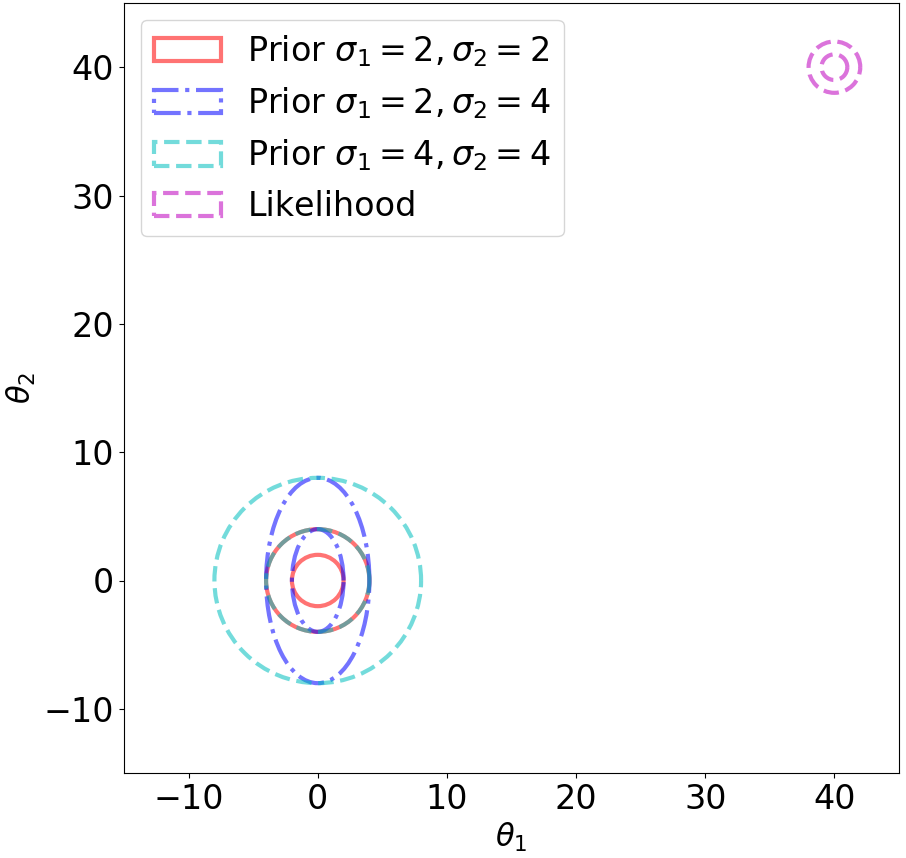
(a) uncorrelated prior

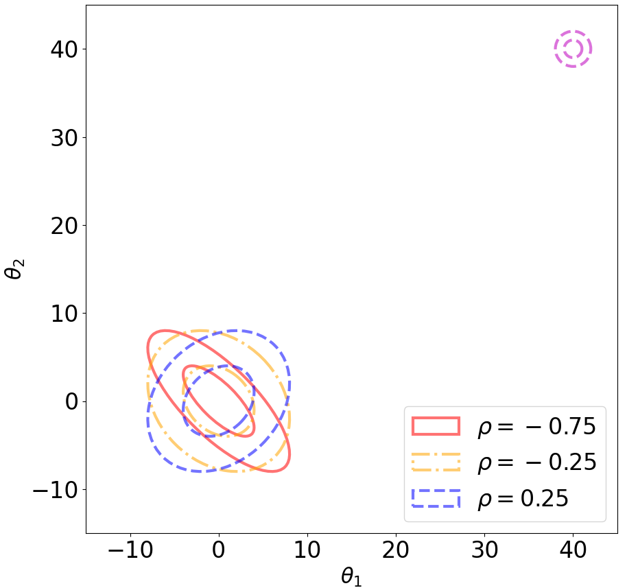
(b) correlated prior

Figure 6: Illustration of the three test cases in the bivariate Gaussian likelihood example with uncorrelated/correlated priors. In the left panel, the cyan dashed, red solid and blue dot-dashed lines denote the Gaussan priors centred on the origin, with $\{\sigma_{\mathbf{\mathit{\theta}}_{1}},\sigma_{\mathbf{\mathit{\theta}}_{2}}\}$ equals to $\{4,4\}$, $\{2,2\}$, and $\{2,4\}$, respectively. The right panel shows correlated prior with $\{4,4\}$ and correlation coefficients $\rho_{\theta}=\{-0.75,-0.25,0.25\}$, respectively, denoted in a rainbow colour order. The pink dashed lines in the upper right corner denote the likelihood distribution. Each distribution contains two coloured contours corresponding to the $2\sigma$ ($68\%$) and $3\sigma$ ($95\%$) iso-probability levels.

Figure 7 is a ‘corner plot’ showing the 1-dimensional and 2-dimensional marginal distributions of the joint ‘effective’ posterior on $(\theta_{1},\theta_{2},\beta)$ for each of the three priors described in Figure 6(a). In each case, the joint posterior again has the form of the product of two independent distributions on $(\theta_{1},\theta_{2})$ and $\beta$, respectively, and is consistent with a marginal on $\beta$ having the approximate form of a top-hat distribution in the range $[0,\beta_{+}]$. One also observes the expected evolution of this marginal across the three test cases, whereby $\beta_{+}$ gradually decreases as the likelihood is concentrated progressively further into the wings of the corresponding prior. Since $\beta_{+}\lesssim 0.1$ in all three cases, one may confirm that each prior is indeed unrepresentative, and one may use the values of $\beta_{+}$ for each case to rank their severity.

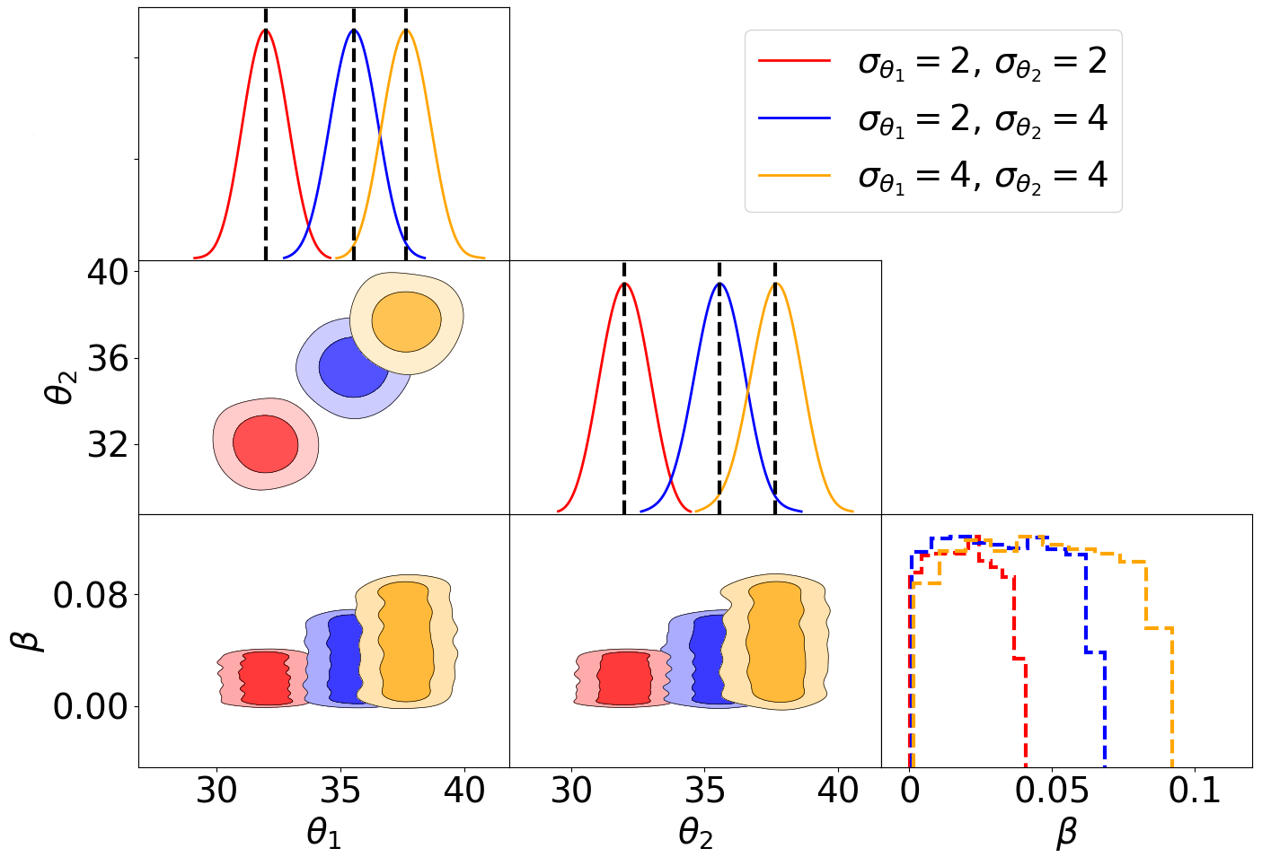
Figure 7: A ‘corner plot’ showing the 1-dimensional and 2-dimensional marginals of the joint posterior distribution on $(\theta_{1},\theta_{2},\beta)$ obtained by MultiNest using BPR for the bivariate Gaussian likelihood example with the likelihood and priors illustrated in Figure 6(a). The vertical dashed black lines indicate the mean of the true Gaussian posterior in each case.

Turning to the marginals on $\mathbf{\mathit{\theta}}_{1}$ and $\theta_{2}$ in Figure 7, one sees that they are correctly centred on the mean of the corresponding true Gaussian posterior for each case. Moreover, the widths of the marginals are stable across the different priors and consistent with the width of the true Gaussian posterior in each case; the RMSE of the $\theta_{\ast}$ estimate $\approx 0.05$ in all cases. Thus, as in the univariate Gaussian likelihood example, the BPR method yields the correct inferences on $(\mathbf{\mathit{\theta}}_{1},\theta_{2})$ without any need for fine tuning.

Table 1: Comparison of the mean and standard deviation of the estimated log-evidence over 10 realisations of the data in the bivariate Gaussian likelihood example, obtained using the BPR method for a selection of uncorrelated priors. The ‘true’ value of the evidence in each case is also given, as estimated using standard quadrature techniques.

Prior	True	BPR	BPR
		mean	s.d.
$\{\sigma_{\mathbf{\mathit{\theta}}_{1}}=4,\sigma_{\mathbf{\mathit{\theta}}_{2}}=4\}$	$-98.79$	$-98.70$	$0.88$
$\{\sigma_{\mathbf{\mathit{\theta}}_{1}}=2,\sigma_{\mathbf{\mathit{\theta}}_{2}}=4\}$	$-182.01$	$-182.01$	$1.24$
$\{\sigma_{\mathbf{\mathit{\theta}}_{1}}=2,\sigma_{\mathbf{\mathit{\theta}}_{2}}=2\}$	$-325.76$	$-325.66$	$1.49$

One may also verify that the BPR method yields accurate evidence estimates in the above cases. Table 1 lists the mean and standard deviation of the estimated log-evidence over 10 realisations of the data for each of the three uncorrelated priors considered; it also lists the corresponding true evidences, estimated using standard quadrature techniques. One sees that in each case the log-evidence estimates obtained using BPR, after making the correction in (16), are all consistent with the true value, and have a standard deviation that remains stable for all the priors considered.

5.2.2 Correlated priors

We now consider priors with fixed standard deviations $\{\sigma_{\mathbf{\mathit{\theta}}_{1}}=4$, $\sigma_{\mathbf{\mathit{\theta}}_{2}}=4\}$, but three typical correlation coefficients $\rho_{\mathbf{\mathit{\theta}}}=\{-0.75,-0.25,0.25\}$. The three prior distributions are illustrated in Figure 6(b), together with the likelihood, from which one can see that all the priors are again unrepresentative.

Figure 8 is a ‘corner plot’ showing the 1-dimensional and 2-dimensional marginal distributions of the joint ‘effective’ posterior on $(\theta_{1},\theta_{2},\beta)$ for each of the three priors described, using the same colour order as in Figure 6(b). As in previous examples, the joint posterior in each case has the expected form of the product of two in independent distributions on $(\theta_{1},\theta_{2})$ and $\beta$, respectively, and the marginal on $\beta$ is consistent with an approximately top-hat distribution in the range $[0,\beta_{+}]$. The evolution of this marginal from $\rho_{\theta}=0.25$ (blue) to $\rho_{\theta}=-0.75$ (red) is as expected, with $\beta_{+}$ gradually decreasing as the likelihood is concentrated further into the wings of the prior distribution, as the latter ‘rotates’ away from the peak of the likelihood. Moreover, since $\beta_{+}\lesssim 0.15$ in every cases, one may conclude that all the priors are indeed unrepresentative and again use the $\beta_{+}$ values to rank their severity.

Figure 8: A ‘corner plot’ showing the 1-dimensional and 2-dimensional marginals of the joint posterior distribution on $(\theta_{1},\theta_{2},\beta)$ obtained by MultiNest using BPR for the bivariate Gaussian likelihood example with the likelihood and priors illustrated in Figure 6(b). The vertical dashed black lines indicate the mean of the true Gaussian posterior.

The marginals on $\mathbf{\mathit{\theta}}_{1}$ and $\theta_{2}$ in Figure 8 are again correctly centred on the corresponding true Gaussian posterior for each case, the means of which are indicated by the vertical black dashed lines. The widths of the marginals are stable across the range of priors and consistent with the width of the true Gaussian posterior in each case; the RMSE of the $\theta_{\ast}$ estimate $\approx 0.06$ in all cases. Hence the inferences on the parameters $(\mathbf{\mathit{\theta}}_{1},\theta_{2})$ using BPR are again accurate and robust in each case, without any tuning.

Table 2: Comparison of the mean and standard deviation of the estimated log-evidence over 10 realisations of the data in the bivariate Gaussian likelihood example, obtained using the BPR method for a selection of priors with $\{\sigma_{\mathbf{\mathit{\theta}}_{1}}=4$, $\sigma_{\mathbf{\mathit{\theta}}_{2}}=4\}$ and correlation coefficient $\rho_{\mathbf{\mathit{\theta}}}$. The ‘true’ value of the evidence in each case is also given, as estimated using standard quadrature techniques.

$\rho_{\mathbf{\mathit{\theta}}}$	True	BPR mean	BPR s.d.
$-0.75$	$-324.39$	$-324.32$	$1.27$
$-0.25$	$-127.72$	$-127.65$	$0.85$
$0.25$	$-80.83$	$-80.75$	$0.98$

One may again verify that the BPR method yields accurate evidence estimates in the above cases. Table 2 lists the mean and standard deviation of the estimated log-evidence values over 10 realisations of the data for each of the three correlated priors considered, and compares them with the corresponding true evidences estimated using standard quadrature techniques. As for the uncorrelated priors, the log-evidence estimates are all consistent with the true value, and have a stable standard deviation across all the priors considered.

5.3 Bivariate multi-modal likelihoods

We now consider bivariate multi-modal likelihoods consisting of an equal mixture of four identical but spatially separated Gaussians. Once again, for the sake of brevity, we consider only an uncorrelated Gaussian prior centred on the origin, with $\sigma_{\theta_{1}}=4$ and $\sigma_{\theta_{2}}=4$. Nonetheless, we do consider two different arrangements of the 4 modes of the likelihood relative to the centre of the prior. In particular we consider the symmetric and asymmetric arrangements illustrated in Figure 9, in which the circles denotes the 3-sigma iso-probability contour of each mode of the likelihood and the prior, respectively. As illustrated, for each arrangement, we consider a range of likelihoods for which the centres of the modes lie at varying distances from the origin. For the symmetric arrangement, each mode lies at the same distance from the origin, with positions ranging from $|\theta_{1}|=|\theta_{2}|=5$ to $|\theta_{1}|=|\theta_{2}|=60$. For the asymmetric arrangement, as shown in Figure 9(b), the centres of the 4 modes are placed a distance of $4$ units from their geometric centre, the position of which ranges from $\theta_{1}=\theta_{2}=5$ to $19$. From Figure 9, one sees that for all the cases considered in the symmetric arrangement the prior is unrepresentative, whereas this is not true for some of the cases considered in the asymmetric arrangement. All other settings are identical to those used in the analysis of the bivariate Gaussian likelihood in Section 5.2.

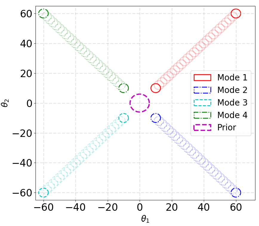
(a) 4-mode symmetric arrangement

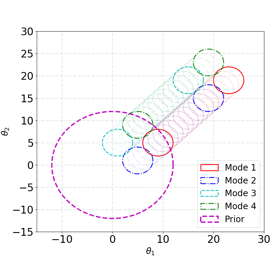
(b) 4-mode asymmetric arrangement

Figure 9: Illustration of the bivariate multimodal likelihoods considered, each of which consists of an equal mixture of four identical spatially-separated Gaussians for: (a) the symmetric arrangement; and (b) the asymmetric arrangement (relative to the prior). In each case, the dashed purple circle (centred at the origin) represents the 3-sigma iso-probability contour of the prior, and the other smaller circles represent the 3-sigma iso-probability contour of each of the four modes.

5.3.1 Symmetric arrangement

Figure 10 summarises the performance of the BPR method in the symmetric arrangements illustrated in Figure 9(a). The upper row of panels (a)-(b) shows the effect of increasing the (equal) distance of the 4 mode centres from the origin for a fixed number of live points $N_{\rm live}=100$. The lower row of panels (c)-(d) shows the effect of increasing the number of live points $N_{\rm live}$ for fixed modes centres at $|\theta_{1}|=|\theta_{2}|=40$.

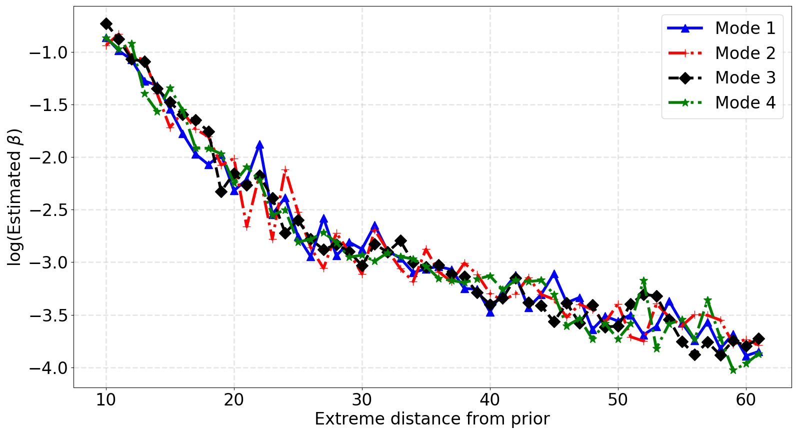
(a) $\log(\beta)$, varying mode distance

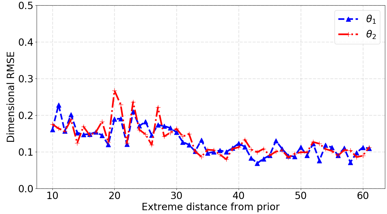
(b) RMSE, varying mode distance

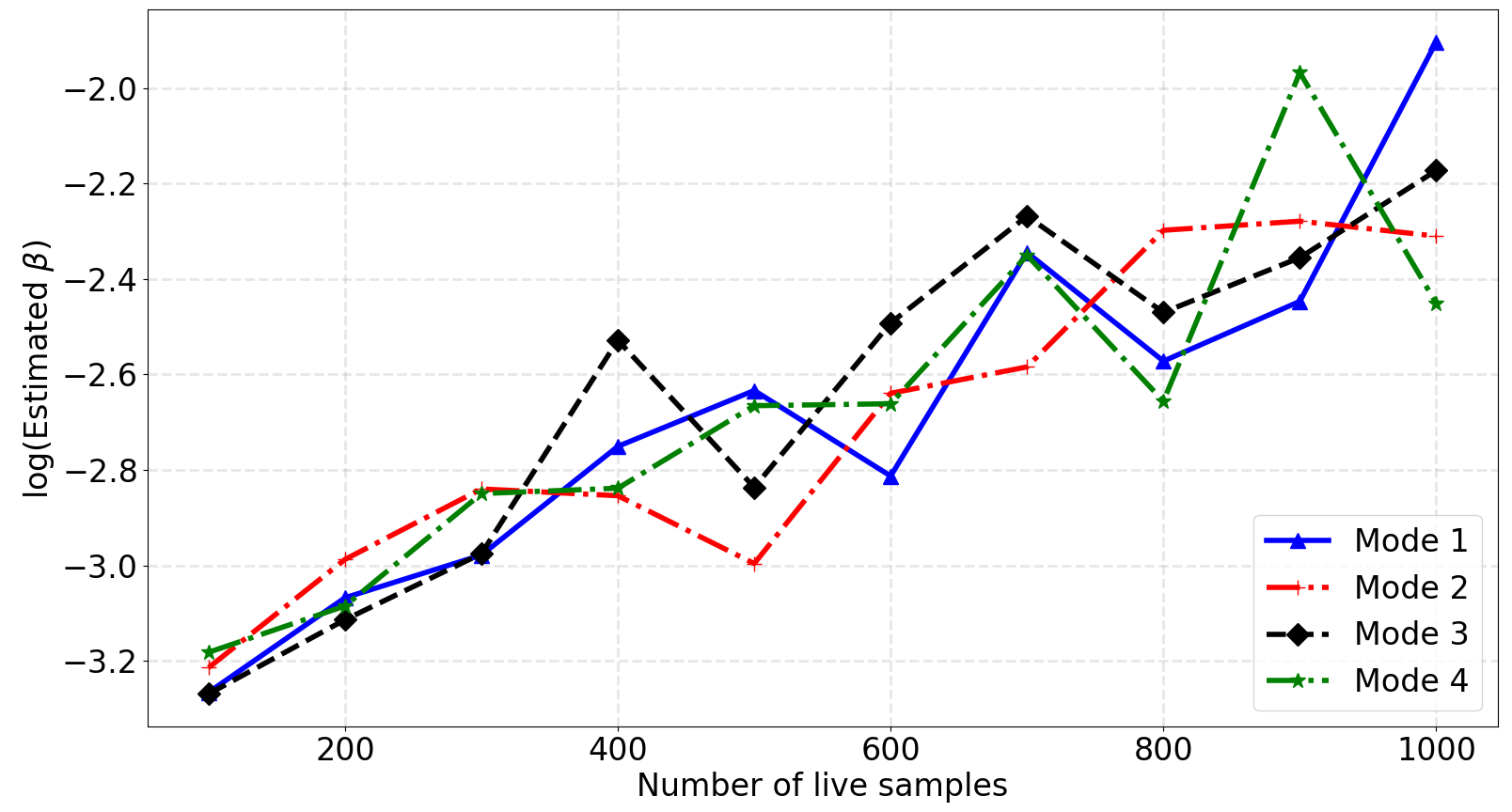
(c) $\log(\beta)$, varying $N_{\rm live}$

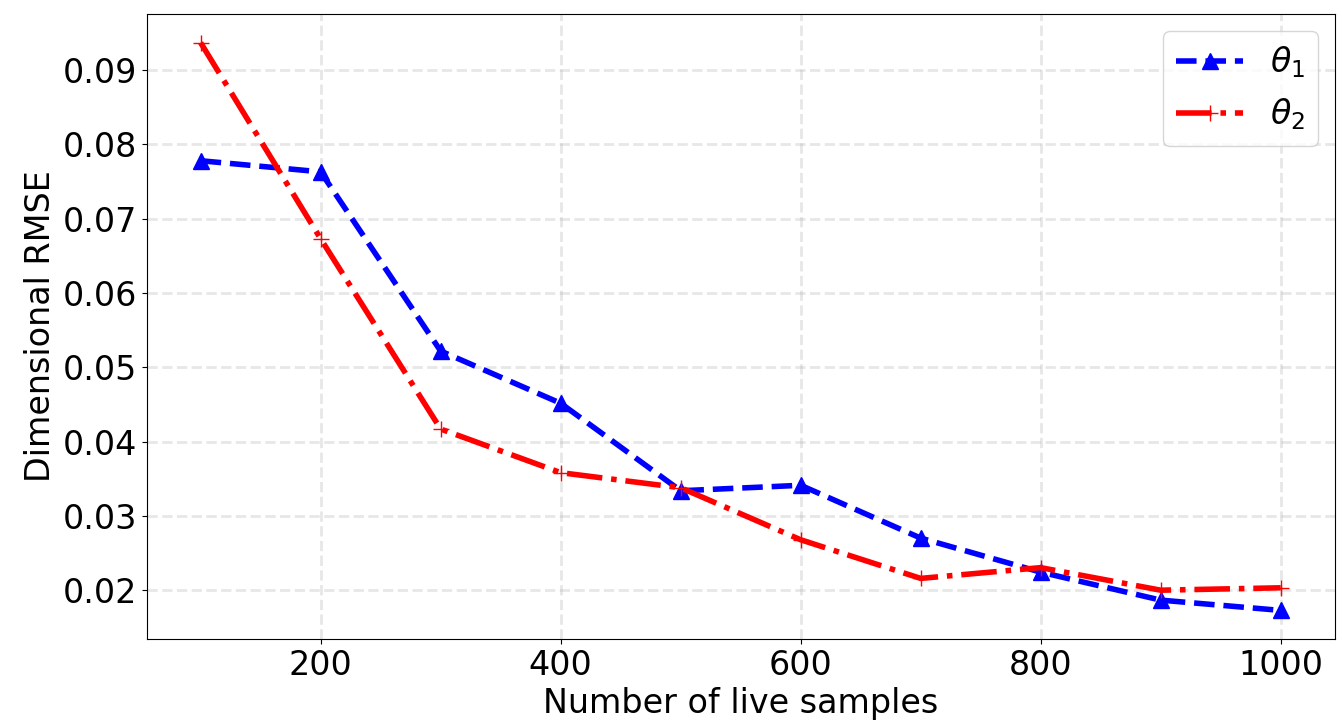
(d) RMSE, varying $N_{\rm live}$

Figure 10: Performance of the BPR method applied to multimodal likelihoods consisting of an equal mixture of 4 identical but spatially-separated Gaussians in the symmetric arrangement illustrated in Figure 9(a). The upper row shows the effect of increasing the (equal) distance of the 4 mode centres from the origin for a fixed number of live points $N_{\rm live}=100$. The lower row shows the effect of increasing the number of live points $N_{\rm live}$ for fixed modes centres at $|\theta_{1}|=|\theta_{2}|=40$. Panels (a) and (c) show $\log(\hat{\beta})$ obtained from posterior samples associated with each of the four modes, separately. Panels (b) and (d) show the RMSE in the estimation of $\theta_{1}$ and $\theta_{2}$, averaged across the 4 modes.

In the left-hand column, i.e. panels (a) and (c), we plot $\log(\hat{\beta})$ (to accommodate the large dynamic range in the estimates of $\hat{\beta}$) obtained from the mean of the posterior samples associated with each of the four modes, separately. In panel (a), the value of $\log(\hat{\beta})$ is consistent across the four modes, as one might expect since they are symmetrically arranged relative to the centre of the prior located at the origin. Moreover, as the (equal) distance of each mode from the origin increases, then the value of $\log(\hat{\beta})$ decreases monotonically (to within the statistical uncertainties of the nested sampling process). In panel (c), one again sees consistency on the values of $\hat{\beta}$ across the four modes, but that $\log(\hat{\beta})$ increases quasi-monotonically as $N_{\rm live}$ increases. This is expected since the failure of the nested sampling algorithm, and the consequent need for the posterior repartitioning characterised by low values of $\beta$, is reduced as $N_{\rm live}$ increases.

In the right-hand column of Figure 10, i.e. panels (b) and (d), we plot the RMSE in the estimation of $\theta_{1}$ and $\theta_{2}$ for each mode, but averaged across the 4 modes. In panel (b), one sees that the RMSE for $\theta_{1}$ and $\theta_{2}$ are consistent, as expected, and that the values remain stable in the range $\sim$ 0.1–0.2 as the (equal) distance of the 4 modes from the origin varies. Panel (d) shows that the RMSE for $\theta_{1}$ and $\theta_{2}$ are again consistent and that these values decrease monotonically as $N_{\rm live}$ increases, as expected.

5.3.2 Asymmetric arrangement

Figure 11 summarises the performance of the BPR method in the asymmetric arrangements illustrated in Figure 9(b), and the quantities displayed in each panel are the same as those in Figure 10. The only differences here are that the panels (a) and (c) show the effects as a function of the distance of the geometric centre of the 4 modes from the origin, and that panels (b) and (d) show the RMSE for each mode separately. Further heatmap illustrations for this example can be found in Figure 15 in the Supplementary Material. This asymmetric modes scenario presents quite an extreme test of the BPR method, but equally illustrates some further key advantages over our original PR method presented in Chen et al. (2018).

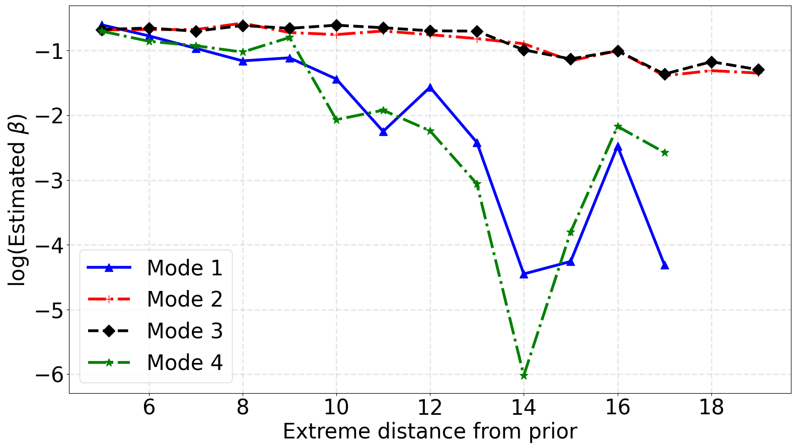
(a) $\log(\beta)$, varying mode distance

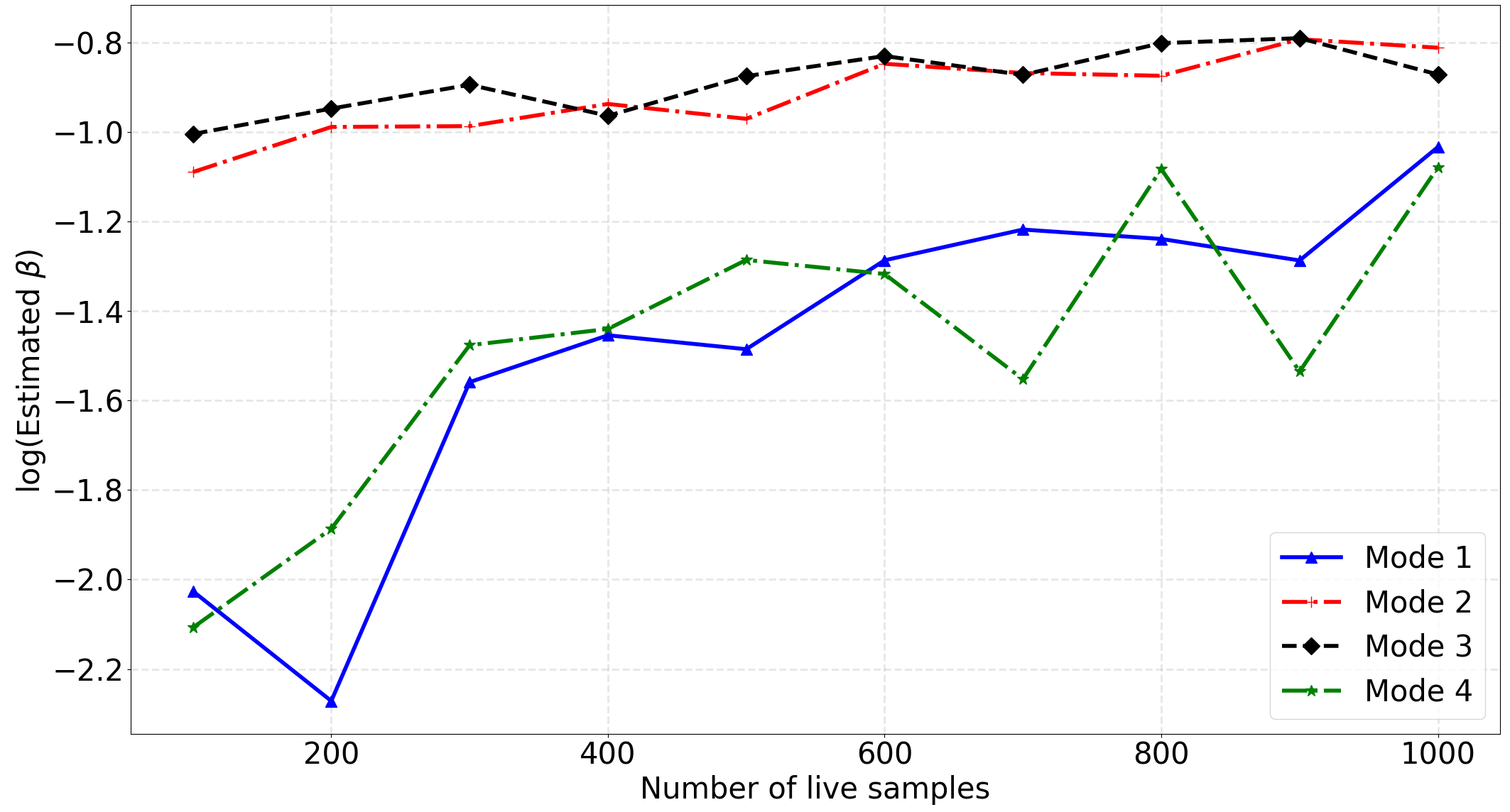
(b) $\log(\beta)$, varying $N_{\rm live}$

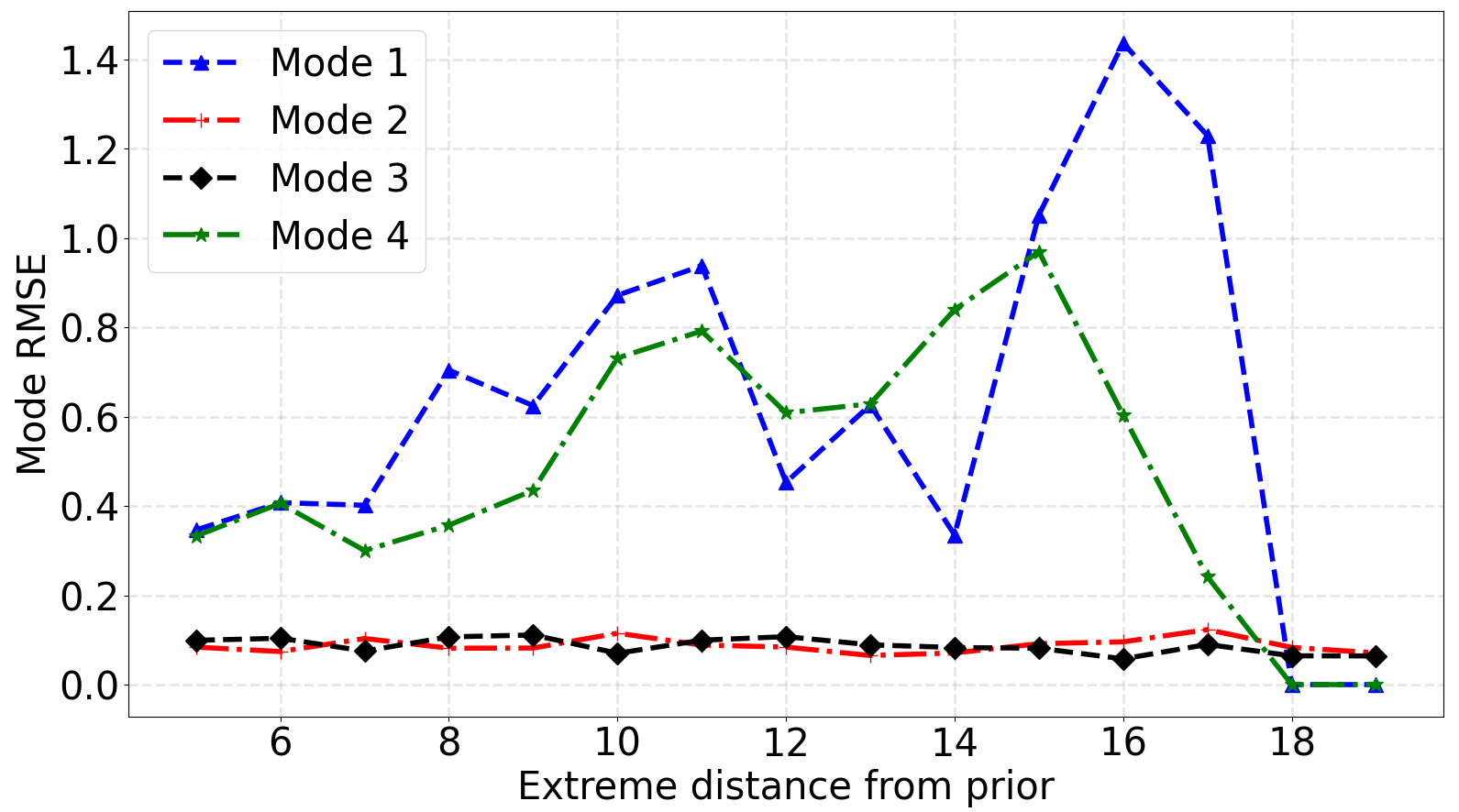
(c) RMSE, varying mode distance

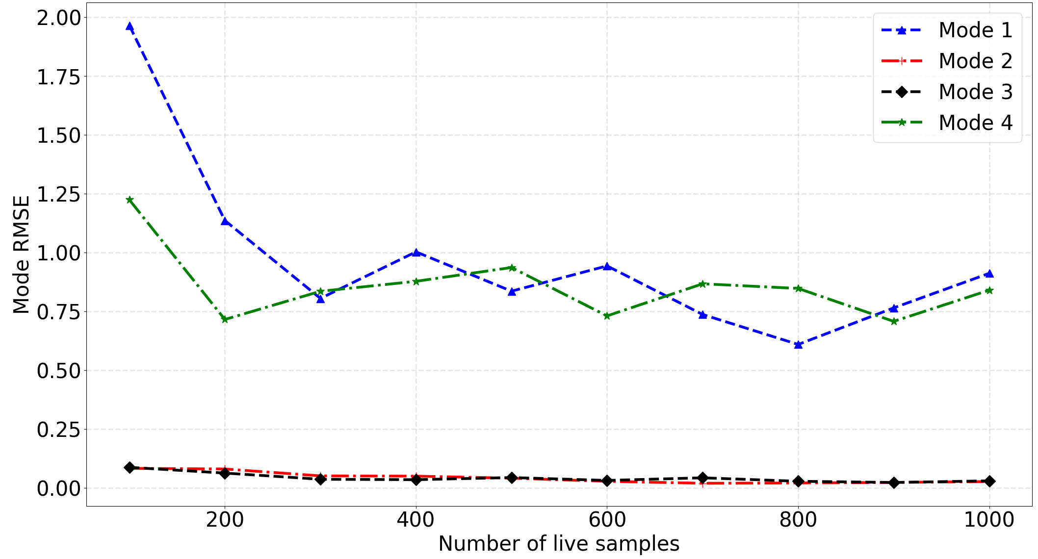
(d) RMSE, varying $N_{\rm live}$

Figure 11: As for Fig 10, but for the asymmetric arrangement illustrated in Figure 9(b). In this case, the panels (a) and (c) show the effects as a function of the distance of the geometric centre of the 4 modes from the origin for $N_{\rm live}=100$, and the panels (b) and (d) show the effects of increasing $N_{\rm live}$ for fixed mode centres, of which the geometric centre is $15$. Also, the panels (c) and (d) show the average RMSE in the estimation of $\theta_{1}$ and $\theta_{2}$ for each mode separately.

A unique feature of BPR in asymmetric multi-modal scenarios: In the upper row of panels (a) and (b), one sees that for each mode the behaviour of $\log(\hat{\beta})$ as a function of distance from the origin and $N_{\rm live}$, respectively, is similar to that found for the symmetric arrangement, and for the same reasons as discussed above. By contrast, however, for the asymmetric arrangement the values of $\log(\hat{\beta})$ are not the same across the 4 modes of the posterior. Instead, the $\log(\hat{\beta})$ values are very similar for modes 2 and 3, and broadly consistent for modes 1 and 4, with the values for the latter pair of modes being much smaller than those for the former pair. By inspecting Figure 9(b), one sees that this is to be expected, since modes 2 and 3 lie closer (but equidistant) from the centre of the prior at the origin, whereas modes 1 and 4 lie further away (but again equidistant). Thus, the prior is more unrepresentative for modes 1 and 4, which thus require a lower value of $\log(\hat{\beta})$.

This demonstrates an important feature of the BPR method, which is not shared by the original PR method, in that different regions of the posterior can be characterised by different ranges of $\beta$ values, depending on how far into the wings of the prior the corresponding regions of likelihood lie, and this is accommodated in a fully automated manner. From panel (a), it is also worth noting that the difference between $\log(\hat{\beta})$ values for modes $(2,3)$ and modes $(1,4)$ is maximal for intermediate distances from the origin. This again makes sense as it corresponds to the point at which there is the largest difference between how representative the prior is for these two sets of modes, since the prior is changing most rapidly between them: for smaller distances (near the peak of the prior) or larger distances (in the wings of the prior), there is less change in the prior between the two sets of modes.

In panels (c) and (d) of Figure 11, one first sees from panel (c) that the average RMSE in the estimation of $\theta_{1}$ and $\theta_{2}$, is low and insensitive to the distance from the origin for modes 2 and 3, which are closer the origin. By contrast, the RMSE is large and more volatile for modes 1 and 4, which lie further into the wings of the prior, and rises slowly with distance from the origin. One sees, however, that the RMSE drops to zero at very large distances; this occurs because, for the default setting of $N_{\rm live}=100$, one obtains no samples in modes 1 and 4. This therefore defines the limit of the applicability of the BPR method in this example, although the issue is resolved by increasing $N_{\rm live}$. In panel (d), one sees that the RMSE is low and insensitive to $N_{\rm live}$ for modes 2 and 3, whereas modes 1 and 4 exhibit a larger and more volatile RMSE, albeit decreasing rapidly up to $N_{\rm live}\approx 300$ and being relatively insensitive to $N_{\rm live}$ thereafter.

5.4 Higher-dimensional Gaussian likelihoods

Finally, we extend the bivariate Gaussian likelihood example in Section 5.2 to higher dimensions from 3D to 10D. We begin by adopting an analogous likelihood, corresponding to $N=1$ data points and centered on $\mathbf{\mathit{\theta}}_{\ast}=40$ in all dimensions, but restrict our analysis to the case of a single circular-symmetric Gaussian prior, with $\sigma_{\mathbf{\mathit{\theta}}}=4$ in all dimensions. Once again, we consider only the BPR results as the standard NS method fails completely in this case. All results presented are based on 10 realisations of the data.

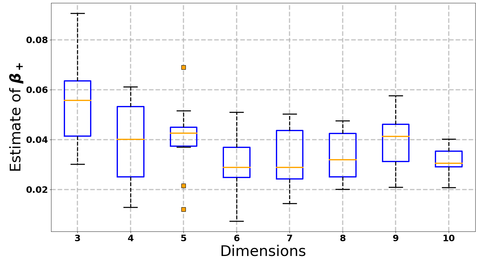
(a) Estimate of $\mathit{\beta}_{+}$

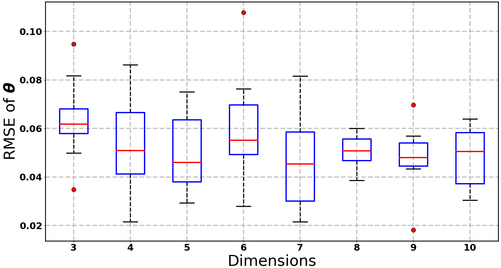
(b) RMSE of $\mathbf{\mathit{\theta}}$ estimate

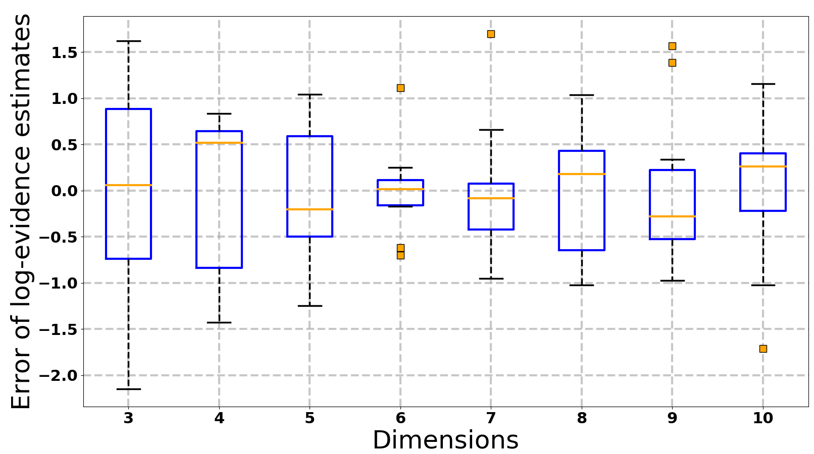
(c) Error of log-evidence estimates

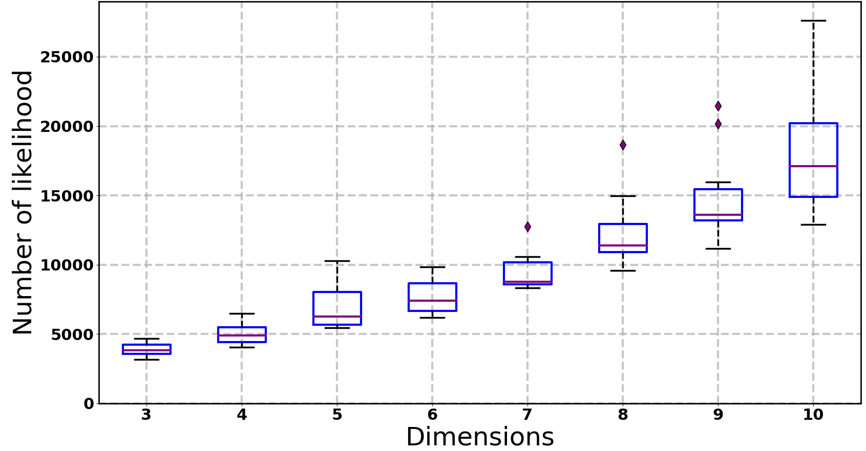
(d) Number of likelihood evaluations

Figure 12: Boxplots for estimated parameter values using the BPR method applied to the higher-dimensional examples with $\mathbf{\mathit{\theta}}_{\ast}=40$, from 3D to 10D. The error bars denote the minimum and maximum values, whereas the boxes indicate the 25th to 75th quantiles. The orange/red line in the box represents the median value over 10 realisations of the data and the points denote outliers.

We first consider the constraints obtained on the parameters $(\bm{\theta},\beta)$. Rather than presenting corner plots of the posterior in these higher dimensionalities, Figure 12(a)-(b) instead shows boxplots of the estimated value of $\beta_{+}$ (the 99% point of the unnormalised marginal posterior $\tilde{P}(\beta)$, as discussed in Section 4) and the RMSE of the estimate of $\theta_{\ast}$ (averaged across all dimensions), as a function of the dimensionality of the problem. The estimated $\beta_{+}$ values are broadly consistent across different dimensionalities, with a mean of $\approx 0.05$ and standard deviation $\approx 0.01$, with only a slight trend to smaller values as the dimensionality increases. This insensitivity to dimensionality is a result of the (effective) joint posterior having the product form (15). Similarly, the RMSE of the $\theta_{*}$ estimate is also seen to be broadly stable across the range of dimensionalities, with a mean value $\approx 0.05$, which is consistent with the accuracy obtained in the bivariate example, and standard deviation $\approx 0.015$.

Turning to the accuracy of the evidence estimates, Figure 12(c) shows a boxplot of the error in the log-evidence, over 10 realisations of the data, as a function of dimensionality. Once again, one sees that the distributions are relatively stable across different dimensionalities, with errors typically lying within one log-unit, which is consistent with the accuracies achieved in the bivariate example.

Finally, we consider the number of likelihood evaluations $N_{\rm like}$ required for MultiNest to converge. Figure 12(d) shows a boxplot of $N_{\rm like}$ over 10 realisations of the data, as a function of dimensionality. The mean value of $N_{\rm like}$ rises from $\sim 3800$ at 3D to $\sim 18100$ at 10D. This trend is consistent with that reported using the original PR method in Chen et al. (2018), and follows roughly an ${\cal O}(n\log n)$ increase with dimensionality. The range of $N_{\rm like}$ values over the 10 realisations is also seen to widen slightly as the number of dimensions increases, but this is a relatively minor effect, at least up to 10D.

6 Conclusions

We have demonstrated that one may straightforwardly automate our previous prior repartitioning method for improving the robustness and efficiency of nested sampling in the presence of an unrepresentative prior. This is achieved by taking an explicitly Bayesian approach that treats the auxiliary parameter $\beta$ in the power PR approach as a hyper-parameter that is estimated alongside the parameters of interest $\bm{\theta}$ of the problem under consideration. Since this estimation process is performed within a single run of the nested sampling algorithm, the BPR method provides a substantial reduction in the computational requirements relative to the annealing schedule approach adopted in the original PR method. In addition to retaining all the advantages of the original scheme in providing reliable parameter constraints and evidence estimates, the BPR method adapts automatically to each problem and thus requires no tuning whatsoever. Indeed, by treating $\beta$ as a hyper-parameter, one may use its resulting marginal to determine both the presence and the severity of an unrepresentative prior. We illustrate these properties in a range of numerical examples, from 1D to 10D, some exhibiting multi-modal likelihoods, with a selection of unrepresentative priors with varying degrees of severity. In particular, for multi-modal likelihoods, we show that different regions of the posterior may be characterised by different values of $\beta$, depending on how far into the wings of the prior the corresponding regions of likelihood lie. Moreover, this is accommodated in a fully automated manner and is an important feature of the BPR method that is not shared by our original PR method.

Perhaps most interestingly, we show that there is negligible computational overhead relative to standard nested sampling when the BPR method is used in cases where the prior is representative, and that it offers significant advantages in terms of efficiency and robustness even if the prior is only marginally unrepresentative. This suggests that the BPR should always be used in the application of nested sampling to Bayesian inference problems, irrespective of whether one suspects that the assumed priors may be unrepresentative for some data sets. Moreover, BPR might usefully be integrated directly into nested sampling algorithms and/or data analysis pipelines. It should be recalled, however, that the computational cost of BPR may be considerably increased if the normalising constant of the modified prior cannot be calculated analytically and so must be estimated numerically.

The authors thank Will Handley and Lukas Hergt for their support with the powerful Python visualisation package anesthetic (Handley, 2019).

7 Supplementary Material

7.1 Nested sampling algorithm

Algorithm 1 describes the pseudo-code for the standard NS algorithm. $X_{i}$ denotes the expected fraction of the prior volume lying within the isolikelihood contour $\mathcal{L}(\bm{\theta})=\mathcal{L}_{i}$ at iteration $i$. In general, the fractional prior volume $X$ lying above some likelihood threshold $\lambda$ is defined as

$$X(\lambda)=\int_{\mathcal{L}(\bm{\theta})>\lambda}\mathit{\pi}(\bm{\theta})d\bm{\theta},$$ (25)

where $\lambda$ gradually rises from the minimum to the maximum of $\mathcal{L}(\bm{\theta})$ as the NS iterations proceed. The NS algorithm provides an estimate of the evidence (3) by casting it as a one-dimensional integral with respect to fractional prior volume $X$:

$$\mathcal{Z}=\int_{0}^{1}\mathcal{L}(X)dX,$$ (26)

subject to the existence of the inverse $\mathcal{L}(X)$ to (25). Finally, tol denotes a pre-defined convergence criterion, which affects the number of NS iterations.

// Nested sampling initialisation

1 At iteration $i=0$:

2 Draw $N_{\rm live}$ samples $\{\bm{\theta}_{n}\}_{n=1}^{N_{\rm live}}$ from prior $\pi(\bm{\theta})$.

3 Initialise evidence $Z=0$ and prior volume $X_{0}=1$.

// NS iterations

4 for $i=1,2,\cdots,I$ do

5       for $n=1,2,\cdots,N_{\rm live}$ do

6             $\bullet$ Compute likelihood $\mathcal{L}(\bm{\theta}_{n})$.

7            

8       end for

9      $\bullet$ Find the lowest likelihood and save in $\mathcal{L}_{i}$.

10       $\bullet$ Calculate weight $w_{i}=\frac{1}{2}(X_{i-1}-X_{i+1})$, where $X_{i}=\exp(-i/N_{\rm live})$

11       $\bullet$ Increment $Z$ by $\mathcal{L}_{i}w_{i}$.

12       $\bullet$ Draw a new sample $\bm{\theta}$ to replace one with likelihood $\mathcal{L}_{i}$, subject to $\mathcal{L}(\bm{\theta})>\mathcal{L}_{i}$.

13       $\bullet$ Stop if $\mbox{max}\{\mathcal{L}(\bm{\theta}_{n})\}X_{i}<{\tt{tol}}\times Z$.

14 end for

15Increment $Z$ by $\sum_{n=1}^{N_{\rm live}}\mathcal{L}(\bm{\theta}_{n})X_{I}/N_{\rm live}$.

16 Assign the sample replaced at iteration $i$ the importance weight $p_{i}=L_{i}w_{i}/Z$.

Algorithm 1 Nested sampling algorithm

7.2 A BPR example with univariate Gaussian likelihood

In this section we further illustrate BPR using the same settings of the univariate Gaussian likelihood in Section 4.1.

In practice, BPR can be easily obtained by modifying the likelihood function (for each example) in standard MultiNest. For the 1D Gaussian example, we have to set the hyper-parameter ‘nDim’ in MultiNest to 2, where the first variable is $\theta$ and the second one is $\beta$ to be estimated.

$\pi(\beta)$ is an uniform distribution $\mathit{\beta}\sim\mathcal{U}[0,1]$, and the original prior $\pi(\mathbf{\mathit{\theta}})$ is a standard Gaussian:

$$\pi(\mathbf{\mathit{\theta}})=(2\pi\sigma_{\mathit{\pi}}^{2})^{\frac{1}{2}}\exp\left(-\frac{(\mathbf{\mathit{\theta}}-\mu_{\mathit{\pi}})^{2}}{2\sigma_{\mathit{\pi}}^{2}}\right)$$ (27)

// Initialisation

1 At iteration $i=0$:

2 Initialise evidence $Z=0$ and prior volume $X_{0}=1$.

3 Draw $N_{\rm live}$ samples $\{\beta_{n}\}_{n=1}^{N_{\rm live}}$ from prior $\pi(\beta)$.

4 Draw $\{\bm{\theta}_{n}\}_{n=1}^{N_{\rm live}}$ samples from prior $\tilde{\pi}(\bm{\theta}|\beta_{n})$, and compute the constant $C$.

5

// BPR iterations

6 for $i=1,2,\cdots,I$ do

7       for $n=1,2,\cdots,N_{\rm live}$ do

8             $\bullet$ Compute likelihood $\tilde{\mathcal{L}}(\bm{\theta}_{n},\beta_{n})$.

9            

10       end for

11      $\bullet$ Find the lowest likelihood and save in $\mathcal{L}_{i}$.

12       $\bullet$ Calculate weight $w_{i}=\frac{1}{2}(X_{i-1}-X_{i+1})$, where $X_{i}=\exp(-i/N_{\rm live})$

13       $\bullet$ Increment $Z$ by $\mathcal{L}_{i}w_{i}$.

14       $\bullet$ Draw a new sample $\bm{\theta}$ to replace one with likelihood $\mathcal{L}_{i}$, subject to $\mathcal{L}(\bm{\theta})>\mathcal{L}_{i}$.

15       $\bullet$ Stop if $\mbox{max}\{\mathcal{L}(\bm{\theta}_{n})\}X_{i}<{\tt{tol}}\times Z$.

16 end for

17Increment $Z$ by $\sum_{n=1}^{N_{\rm live}}\mathcal{L}(\bm{\theta}_{n})X_{I}/N_{\rm live}$.

18 Assign the sample replaced at iteration $i$ the importance weight $p_{i}=L_{i}w_{i}/Z$.

Algorithm 2 BPR 1D Gaussian example

The modified prior and likelihood can then be derived:

$$\tilde{\mathit{\pi}}(\bm{\theta}|\beta) = \frac{\mathit{\pi}(\bm{\theta})^{\mathit{\beta}}}{\mathcal{Z}_{\pi}(\beta)},$$ (28)

$$\tilde{\mathcal{L}}(\bm{\theta},\beta) = \mathcal{L}(\bm{\theta})\mathit{\pi}(\bm{\theta})^{(1-\mathit{\beta})}\mathcal{Z}_{\pi}(\beta),$$ (29)

We can easily obtain an unnormalised powered distribution:

$$\mathit{\pi}(\bm{\theta})^{\mathit{\beta}}=(2\pi)^{\frac{\beta}{2}}\sigma_{\mathit{\pi}}^{\beta}\exp\left(-\frac{(\mathbf{\mathit{\theta}}-\mu_{\mathit{\pi}})^{2}}{2(\frac{\sigma_{\mathit{\pi}}}{\sqrt{\beta}})^{2}}\right),$$ (30)

which is equivalent to designing a new Gaussian distribution $\mathcal{N}(\mu_{\mathit{\pi}},(\frac{\sigma_{\mathit{\pi}}}{\sqrt{\beta}})^{2})$ by multiplying a constant $C=(2\pi)^{\frac{1-\beta}{2}}\sigma_{\mathit{\pi}}^{1-\beta}\beta^{-\frac{1}{2}}$. $\mathcal{Z}_{\pi}(\beta)$ is the normalising constant and can be easily computed by finite summation from drawn samples. Therefore, the newly designed Gaussian distribution forms the modified prior $\tilde{\mathit{\pi}}(\bm{\theta}|\beta)$.

The pseudo code is shown in Algorithm 2. In each iteration for the $n$th live point, BPR will draw a $\beta_{n}$, and convert sample $\mathbf{\mathit{\theta}}_{n}$ (which is originally drawn from the unit hypercube) to the modified Gaussian $\tilde{\mathit{\pi}}(\bm{\theta}|\beta)$. $\mathit{\pi}(\bm{\theta})^{(1-\mathit{\beta})}$ can also be easily computed following the same rule and finally the modified log-likelihood $\log\tilde{\mathcal{L}}(\bm{\theta},\beta)$ can be computed by summing up the logarithm of the terms in Eqn. (29).

7.3 More results for the univariate Gaussian likelihood example

Figure 13 shows the (logarithm of the) root mean squared error (RMSE) of the estimate $\hat{\mathbf{\mathit{\theta}}}$ over 10 realisations of the data for each value of $\mathbf{\mathit{\theta}}_{\ast}$, for both the standard NS approach and the BPR method. one sees that the RMSE of $\hat{\mathbf{\mathit{\theta}}}$ for the standard NS approach rapidly increases for $\theta_{\ast}\gtrsim 20$, as the prior $\pi(\theta)$ becomes increasingly unrepresentative and the NS algorithm begins to fail, but that the RMSE of the BPR method remains stable as $\theta_{\ast}$ increases, indicating robust parameter estimation in all cases. Moreover, for $\theta_{\ast}\lesssim 15$, the RMSE of BPR is consistent with that of the standard NS approach, demonstrating that there is no reduction in estimation accuracy associated with the BPR method in analysing datasets for which the prior is representative. This is an important conclusion, since it suggests that one sacrifices nothing in terms of parameter estimation accuracy by always using the BPR method, which also has the advantage that one stands to gain considerably from its use when one (unexpectedly) encounters a dataset for which the prior is unrepresentative.

As we discussed in Section 1, the failure of standard NS, which occurs in this example around $\mathbf{\mathit{\theta}}_{\ast}=15$ to $20$, is associated with the issue of likelihood values being indistinguishable to machine precision. For double precision arithmetic, the smallest number that can be represented is $\sim 10^{-308}\sim e^{-709}$. For a Gaussian distribution $\sim\exp(-d^{2}/2)$, where $d$ is Mahalanobis distance, this corresponds to $d\sim 37$. In this example, the Gaussian likelihood has width $\sim 0.22$, so that the ‘basin of attraction’ of the likelihood, which is defined by where likelihoods become zero to machine precision corresponds to a distance $\sim 37\times 0.22\approx 8$ units from its centre. Turning to the Gaussian prior centred on zero, one would expect one of the $N_{\rm live}=100$ samples to lie beyond a distance of $\sim 2.5\sigma_{\pi}=10$. Thus, one expects one of the samples from the prior to lie within the basin of attraction of the likelihood provided its centre does not lie beyond $\sim~{}10+8=18$ units, which agrees well with the numerical results. This simple argument should be refined to take into account that, in total, one draws $N_{\rm like}$ samples from the prior during the full NS run, which is typically considerably larger than $N_{\rm live}$, and depends on the convergence criterion used. Even if $N_{\rm like}\sim 10^{4}$, however, one would expect one of the samples to lie beyond a distance of only $\sim 3.5\sigma_{\pi}=14$, so that the standard NS should fail when the likelihood centre lies beyond $\sim 14+8=22$ units, which is again consistent with the numerical results.

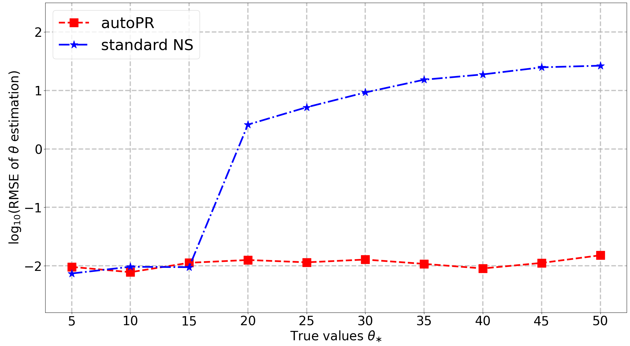
(a) Log₁₀(RMSE) of $\hat{\mathbf{\mathit{\theta}}}$

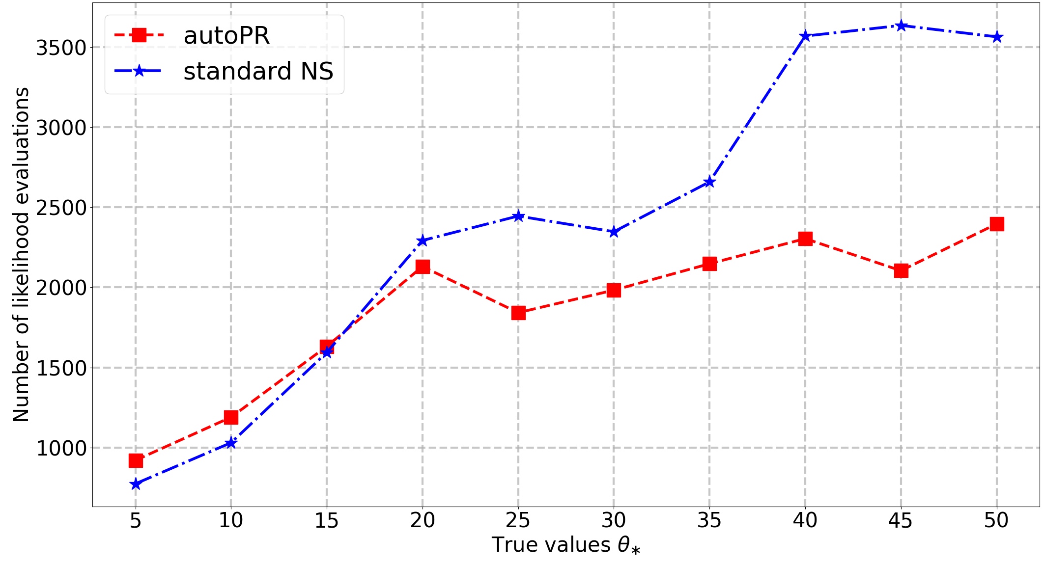
(b) Number of likelihood evaluations

Figure 13: Algorithm performance comparison in the univariate Gaussian likelihood example over 10 realisations of the data for each value of $\mathbf{\mathit{\theta}}_{\ast}$. The left panel shows Log₁₀(RMSE) of the estimate $\hat{\mathbf{\mathit{\theta}}}$, and the right panel shows the mean number of likelihood evaluations, both of which are obtained using the standard NS approach (blue star points) and the BPR method (red square points).

To demonstrate further the practicality of always using the BPR method, Figure 13(b) shows the mean number of likelihood evaluations performed by MultiNest over 10 realisations as a function of $\mathbf{\mathit{\theta}}_{\ast}$, for both the standard NS and BPR methods. One sees that both methods require similar numbers of likelihood evaluations for $\mathbf{\mathit{\theta}}_{\ast}\lesssim 20$, demonstrating that there is very little additional computational overhead resulting from extending the parameter space (in this case doubling its dimensionality) to include the extra hyperparameter $\beta$. Moreover, for larger values of $\mathbf{\mathit{\theta}}_{\ast}$, the number of likelihood evaluations required by the standard NS approach continues to increase with $\mathbf{\mathit{\theta}}_{\ast}$, whereas the number required by the BPR method remains roughly constant. This again suggests that one should use the BPR method in all applications of NS.

One may also compare the accuracy of the standard NS algorithm and the BPR method in estimating evidences. Table 3 lists the mean and standard deviation of the estimated log-evidence over 10 realisations of the data for each method, for each considered value of $\theta_{\ast}$. The table also lists the ‘true’ value of the evidence in each case, estimated using standard quadrature techniques. One sees that for the standard NS approach, the log-evidence estimates quickly become increasingly biased and volatile as $\theta_{\ast}$ increases. By contrast, the log-evidence estimates obtained using BPR, after making the correction in (16), are all consistent with the true value, and have a standard deviation that remains stable for all values of $\mathbf{\mathit{\theta}}_{\ast}$. This once again suggests that one should always using the BPR method, since the required accuracy in evidence estimation is achieved even for datasets for which the prior is representative.

Table 3: Comparison of the mean and standard deviation of the estimated log-evidence over 10 realisations of the data, obtained using standard NS (SNS) and the BPR method, for a range of $\theta_{\ast}$ values in the univariate Gaussian likelihood example. The ‘true’ value of the evidence in each case is also given, as estimated using standard quadrature techniques.

$\theta_{\ast}$	True	BPR mean	SNS mean	BPR s.d.	SNS s.d.
5	$-22.04$	$-21.99$	$-22.03$	0.18	0.04
10	$-24.38$	$-24.28$	$-24.81$	0.21	1.30
15	$-28.27$	$-28.10$	$-86.78$	0.24	103.76
20	$-33.73$	$-33.66$	$-222.50$	0.27	297.00
25	$-40.73$	$-40.64$	$-463.27$	0.27	434.38
30	$-49.30$	$-49.29$	$-1319.58$	0.28	1281.99
35	$-59.43$	$-59.38$	$-2530.09$	0.29	1631.83
40	$-71.11$	$-71.00$	$-4309.03$	0.30	2714.91
45	$-84.35$	$-84.29$	$-6963.08$	0.30	3327.04
50	$-99.15$	$-99.07$	$-10604.46$	0.31	3816.67

Table 4 compares the number of ‘effective’ posterior samples against the number of likelihood evaluations for $N_{\rm live}=100$ in the same Gaussian example. One sees that both $N_{\rm eff}$ and $N_{\rm like}$ are comparable in the case $\theta_{\ast}=5$, where the true value lies within the range of Gaussian prior $\theta\sim\mathcal{N}(0,4^{2})$. Both ratios decrease as the prior becomes increasingly unrepresentative, but the ratio for standard NS reduces almost to zero, with only one ‘effective’ sample in the extreme case $\theta_{\ast}=50$. By contrast, BPR maintains a steady ‘effective’ posterior sample number and ratio across all cases.

Table 4: Comparison of the ‘effective’ posterior samples between BPR and the standard MultiNest. All results are averaged over 10 realisations. $\theta_{\ast}$ represents the true value of $\theta$. $N_{\rm eff}$ is the number of ‘effective’ posterior samples, $N_{\rm like}$ is the total number of likelihood evaluations. Ratio equals to $N_{\rm eff}$ divided by $N_{\rm like}$.

$\theta_{\ast}$	BPR $N_{\rm eff}$	BPR $N_{\rm like}$	BPR ratio	NS $N_{\rm eff}$	NS $N_{\rm like}$	NS ratio
5	$307$	$857$	$35.8\%$	$278$	$742$	$37.5\%$
10	$371$	$1233$	$30.1\%$	$279$	$1008$	$27.7\%$
20	$456$	$2268$	$20.1\%$	$356$	$2576$	$13.8\%$
30	$451$	$1918$	$23.5\%$	$331$	$4513$	$7.3\%$
40	$434$	$1979$	$21.9\%$	$298$	$4361$	$6.8\%$
50	$495$	$2275$	$21.8\%$	$1$	$5559$	$0.017\%$

We conclude our discussion of this first numerical example by performing a comparison between BPR and our original PR method (Chen et al., 2018), in order to illustrate some of the advantages of the former, as outlined in Section 4. In particular, we consider the extreme example of the univariate Gaussian likelihood with $\mathbf{\mathit{\theta}}_{\ast}=40$, again using $N_{\rm live}=100$ live points (note that this is somewhat fewer than $N_{\rm live}=2000$ used in the analysis of the same example first presented in Chen et al. (2018)). For simplicity, we adopt a simple linear ‘annealing schedule’ for the original PR method, reducing $\beta$ from unity (which corresponds to standard NS) in steps of 0.1. Since the dispersion of the RMSE is quite large for $N_{\rm live}=100$, especially for $\beta\geq 0.6$ where the NS process may fail completely, it is difficult to identify convergence of the statistical inferences as $\beta$ is reduced. Consequently, it is necessary to repeat the analysis 10 times for each value of $\beta$, in order for the convergence to be reliably determined. The resulting RMSE of $\hat{\mathbf{\mathit{\theta}}}$ and the number of likelihood evaluations at each value of $\beta$, both averaged over the 10 analyses, are listed in Table 5. One sees that convergence occurs for $\beta\leq 0.2$, which is consistent with the upper limit $\beta_{+}\approx 0.15$ of the effective marginalised posterior $\tilde{\mathcal{P}}(\beta)$ plotted in Figure 5. Turning to the average number of likelihood evaluations, one first notes that $N_{\rm like}$ diverges from the overall decreasing trend for $\beta\geq 0.7$; this occurs since the NS algorithm erroneously terminates early for large $\beta$ values in this example of an extreme unrepresentative prior. For $\beta\leq 0.6$, $N_{\rm like}$ then decreases monotonically, before converging for $\beta\leq 0.2$ to a value consistent with $N_{\rm like}$ required in the BPR method. Nonetheless, the total number of likelihood evaluations required by the original PR method across the 10 analyses at each $\beta$ value is more than two orders of magntiude greater than that required by the BPR method, which demonstrates the considerable improved effectiveness of the latter.

Table 5: The RMSE of $\hat{\mathbf{\mathit{\theta}}}$ and the number of likelihood evaluations at each considered value of $\beta$ in a linear ‘annealing schedule’ for the original PR method with $N_{\rm live}=100$ applied to the extreme example of the univariate Gaussian likelihood with $\mathbf{\mathit{\theta}}_{\ast}=40$. All results are averaged over 10 realisations of the data.

$\beta$ value	$\hat{\mathbf{\mathit{\theta}}}$ RMSE	$N_{\rm like}$
PR(0.9)	$38.5533$	$2312$
PR(0.8)	$26.5783$	$2687$
PR(0.7)	$18.4579$	$2558$
PR(0.6)	$4.3242$	$5413$
PR(0.5)	$2.8731$	$4414$
PR(0.4)	$2.3016$	$4339$
PR(0.3)	$1.8950$	$4005$
PR(0.2)	$0.0087$	$2482$
PR(0.1)	$0.0088$	$2421$
BPR ($\beta_{+}\approx 0.15$)	$0.0090$	$2304$

7.4 Bivariate Laplace likelihood example

We now consider an example in which the bivariate Gaussian likelihood used in Section 5.2 is replaced with a bivariate likelihood based on the Laplace distribution in order to investigate the performance of the BPR method in the presence of fatter tails and a cusp at the likelihood peak. In particular, we consider a bivariate likelihood that is the product of two identical univariate Laplace likelihoods of the form

$$\mathcal{L}(\mathbf{\mathit{\theta}})=\prod_{n=1}^{N}\left\{\frac{1}{2b}\exp\left(-\frac{|\mathbf{\mathit{\theta}}-m_{n}|}{b}\right)\right\},$$ (31)

where the location parameter is represented by the $n$th measurement $m_{n}$ and $b$ is the scale parameter, which is analogous to $\sigma_{\xi}$ in the Gaussian distribution in (18). In this example, we take the scale parameter value to be $b=0.1$ to produce a narrow, steep Laplace distribution. One should note that a bivariate Laplace distribution constructed in this way is not circularly symmetric and differs from the usual form adopted for multivariate Laplace distributions (Kotz et al., 2001). Once again, we consider just $N=1$ measurement to facilitate a straightforward comparison with the bivariate Gaussian likelihood example in the previous section.

For the sake of brevity, we consider only one of the priors used in the previous section, namely an uncorrelated Gaussian prior centred on the origin, with $\sigma_{\theta_{1}}=4$ and $\sigma_{\theta_{2}}=4$. We do, however, consider 8 different centerings of the likelihood, for which the true values are $\bm{\theta}_{\ast}=(\theta_{1},\theta_{2})^{\top}$, where $\theta_{1}=\theta_{2}=5,10,15,20,25,30,35$ and $40$, respectively, so that the peak of the likelihood moves progressively further from the origin. All other settings are identical to those used for the bivariate Gaussian bivariate likelihood example in the previous section; in particular, we perform the analysis over 10 realisations of the data for each of the 8 likelihood centres considered.

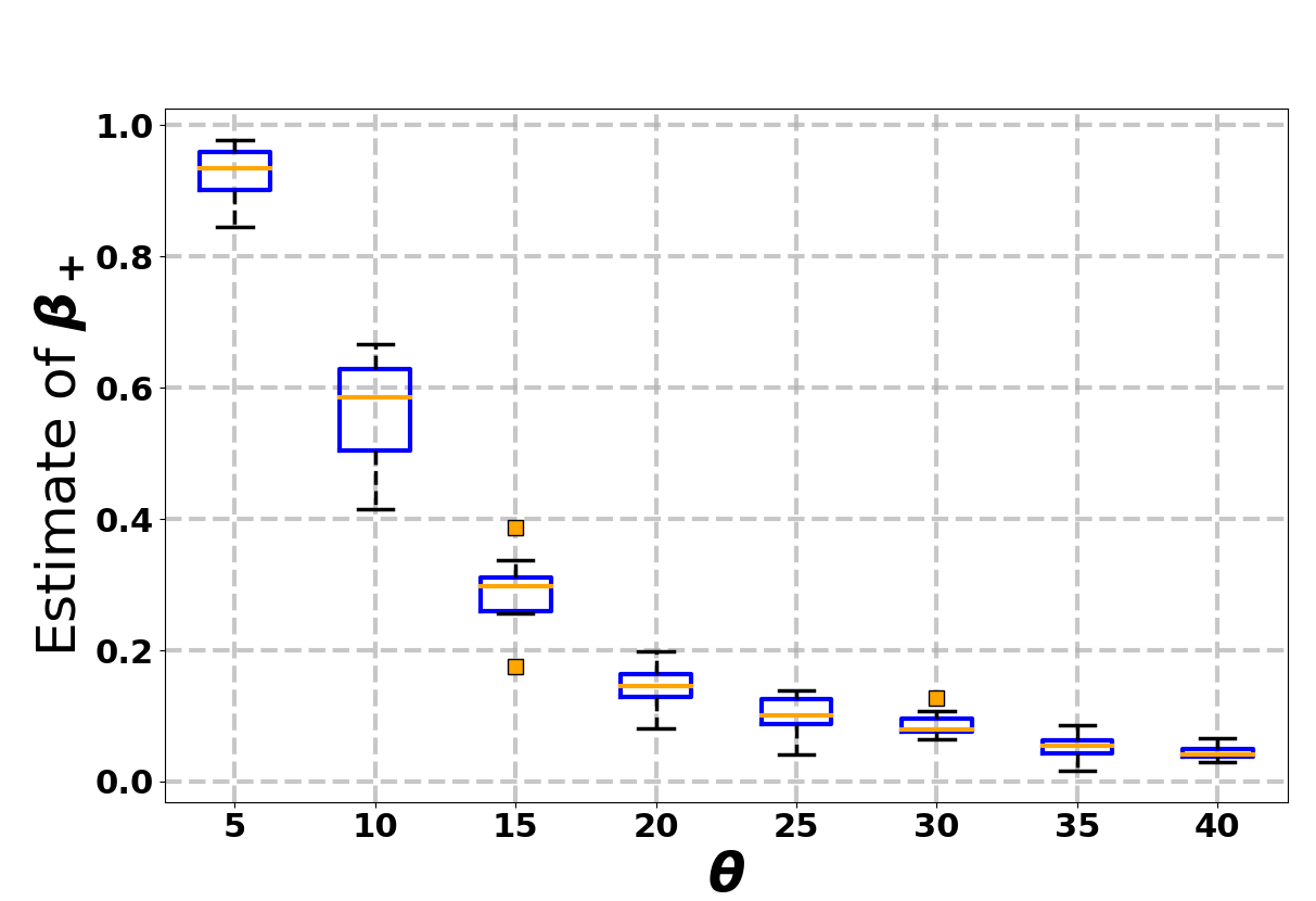
(a) Estimation of $\beta_{+}$

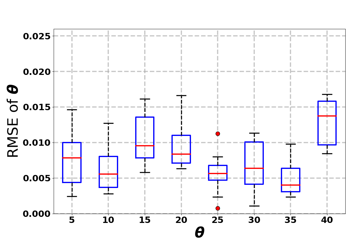
(b) RMSE of $\mathbf{\mathit{\theta}}$ estimation

(c) Error of log-evidence estimates

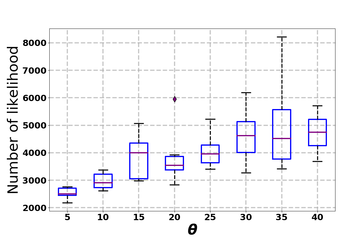
(d) Number of likelihood evaluations

Figure 14: Boxplots for estimated parameter values using the BPR method applied to the bivariate Laplace likelihood example, with $\bm{\theta}_{\ast}$ ranging from $(5,5)$ to $(40,40)$, and an uncorrelated Gaussian prior centred on the origin with $\sigma_{\theta_{1}}=4$ and $\sigma_{\theta_{2}}=4$. The extent of each box denotes the first and third quartiles, $Q_{1}$ and $Q_{3}$, of the 10 realisations of the data considered, and the error bars denote the ‘minimum’ and ‘maximum’ values, defined as $Q_{1}-\tfrac{3}{2}(Q_{3}-Q_{1})$ and $Q_{3}+\tfrac{3}{2}(Q_{3}-Q_{1})$, respectively. The line in each box represents median value (or second quartile $Q_{2}$) and the circles and squares denote any ‘outliers’ that lie beyond the ‘minimum’ and ‘maximum’.

Figure 14 summarises the resulting performance of the BPR method in an alternative format to that used in the previous section, which makes use of boxplots. Figure 14(a) illustrates the estimation of $\beta_{+}$ (the upper limit of the marginal posterior on $\beta$) as a function of the true value $\bm{\theta}_{\ast}$ assumed. As expected, one sees a monotonic decline in the estimated $\beta_{+}$ value as $\bm{\theta}_{\ast}$ increases, indicating that the prior becomes increasingly unrepresentative. Moreover, one sees that the range of $\beta_{+}$ estimates over the 10 realisations of the data is stable for each of the 8 cases considered. Figure 14(b) shows an analogous plot for the RMSE of the estimate of $\bm{\theta}_{\ast}$, which is calculated as the average of the RMSE of $\mathbf{\mathit{\theta}}_{1}$ and $\theta_{2}$. The RMSE values typically lie in the range 0.005–0.01, which indicates that the BPR method provides an accurate estimate in all cases. Figure 14 (c) shows the error in the estimate of the log-evidence, which is centred on zero in all cases, showing that evidence estimates are unbiassed. Moreover, the accuracy of the log-evidence estimates is typically $\sim 0.3$, but with the occasionally outlier having an estimation error up to $\sim 1$; this is broadly consistent with the accuracies of the log-evidence estimates for the bivariate Gaussian likelihood example listed in Table 2. Finally, Figure 14 (d) shows the number of likelihood evaluations $N_{\rm like}$ required for MultiNest to converge using the BPR method, which gradually increases with $\bm{\theta}_{\ast}$ as is expected for progressively more unrepresentative priors. Nonetheless, the rate of increase in $N_{\rm like}$ is relatively slow, showing that the BPR method is computationally feasible, even for extreme unrepresentative priors in the presence of likelihoods with fat tails and a cusp at its peak.

7.5 More results for the bivariate multi-modal likelihoods example

In Figure 15, one sees that the percentage of equally weighted posterior samples is far larger for modes 2 and 3 than for modes 1 and 4, as expected. From panel (a), the percentage of samples in modes 1 and 4 drops gradually, again as expected, from a few percent, when the extreme distance from the origin is 5 units, down to zero for 18 units and beyond, for the default value of $N_{\rm live}=100$. From panel (b), one sees that the percentage of samples in modes 1 and 4 is relatively insensitive to $N_{\rm live}$, with around 0.02% of samples lying in each mode.

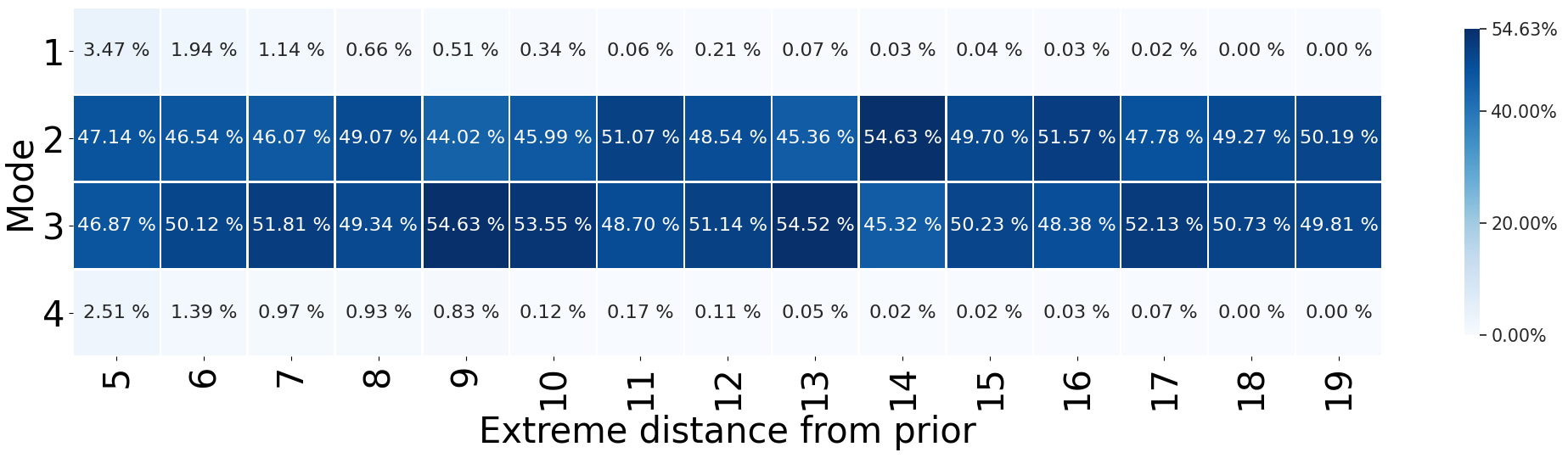
(a) Heat-map, varying mode distance

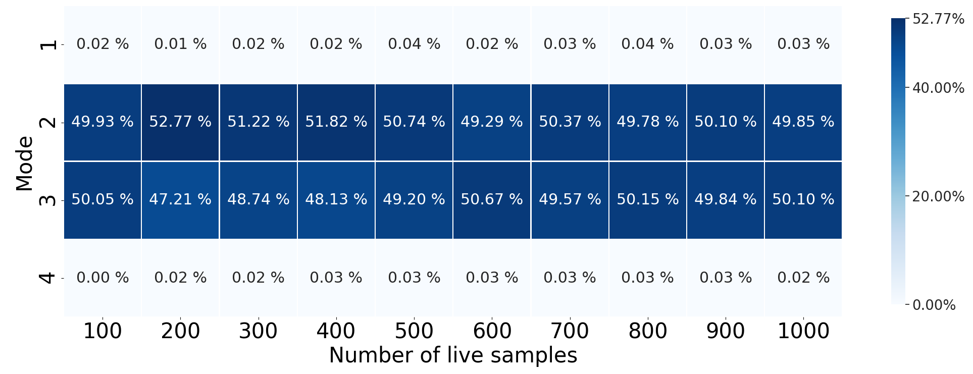
(b) Heat-map, varying $N_{\rm live}$

Figure 15: The heatmap of the asymmetric arrangement bivariate multi-modal case. The panel (e) shows the effect as a function of the distance of the geometric centre of the 4 modes from the origin for $N_{\rm live}=100$, and the panels (f) show the effects of increasing $N_{\rm live}$ for fixed mode centres, with the geometric centre of the modes centred at $\theta_{1}=\theta_{2}=15$.

References

- Alsing and Handley (2021) Alsing, J. and Handley, W. (2021). “Nested sampling with any prior you like.” arXiv e-prints, arXiv:2102.12478.
- Baldock et al. (2017) Baldock, R. J., Bernstein, N., Salerno, K. M., Pártay, L. B., and Csányi, G. (2017). “Constant-pressure nested sampling with atomistic dynamics.” Physical Review E, 96(4): 043311.
- Brewer et al. (2011) Brewer, B. J., Pártay, L. B., and Csányi, G. (2011). “Diffusive nested sampling.” Statistics and Computing, 21(4): 649–656.
- Buchner (2019) Buchner, J. (2019). “Collaborative nested sampling: Big Data versus complex physical models.” Publications of the Astronomical Society of the Pacific, 131(1004): 108005.
- Buchner (2021) — (2021). “Nested Sampling Methods.” arXiv preprint arXiv:2101.09675.
- Chen et al. (2018) Chen, X., Hobson, M., Das, S., and Gelderblom, P. (2018). “Improving the efficiency and robustness of nested sampling using posterior repartitioning.” Statistics and Computing, 1–16.
- Chopin and Robert (2007) Chopin, N. and Robert, C. (2007). “Contemplating evidence: properties, extensions of, and alternatives to nested sampling.” Technical report, Technical Report 2007-46, CEREMADE, Université Paris Dauphine.
- Feroz and Hobson (2008) Feroz, F. and Hobson, M. (2008). “Multimodal nested sampling: an efficient and robust alternative to Markov Chain Monte Carlo methods for astronomical data analyses.” Monthly Notices of the Royal Astronomical Society, 384(2): 449–463.
- Feroz et al. (2009) Feroz, F., Hobson, M., and Bridges, M. (2009). “MultiNest: an efficient and robust Bayesian inference tool for cosmology and particle physics.” Monthly Notices of the Royal Astronomical Society, 398(4): 1601–1614.
- Feroz et al. (2013) Feroz, F., Hobson, M., Cameron, E., and Pettitt, A. (2013). “Importance nested sampling and the MultiNest algorithm.” arXiv preprint arXiv:1306.2144.
-
Handley (2019)
Handley, W. (2019).
“anesthetic: nested sampling visualisation.”
The Journal of Open Source Software, 4(37).
URL http://dx.doi.org/10.21105/joss.01414 - Handley et al. (2015) Handley, W., Hobson, M., and Lasenby, A. (2015). “POLYCHORD: next-generation nested sampling.” Monthly Notices of the Royal Astronomical Society, 453(4): 4384–4398.
-
Higson et al. (2018)
Higson, E., Handley, W., Hobson, M., and Lasenby, A. (2018).
“Dynamic nested sampling: an improved algorithm for parameter
estimation and evidence calculation.”
Statistics and Computing.
URL https://doi.org/10.1007/s11222-018-9844-0 -
Kotz et al. (2001)
Kotz, S., Kozubowski, T., and Podgorski, K. (2001).
The Laplace Distribution and Generalizations: A Revisit with
Applications to Communications, Economics, Engineering, and Finance.
Progress in Mathematics. Birkhäuser Boston.
URL https://books.google.co.uk/books?id=cb8B07hwULUC - MacKay (2003) MacKay, D. (2003). Information theory, inference and learning algorithms. Cambridge university press.
- Skilling (2006) Skilling, J. (2006). “Nested Sampling for General Bayesian Computation.” Bayesian Analysis, 1(4): 833–860.
- Speagle (2020) Speagle, J. S. (2020). “dynesty: a dynamic nested sampling package for estimating Bayesian posteriors and evidences.” Monthly Notices of the Royal Astronomical Society, 493(3): 3132–3158.