Non-Equilibrium Spectrum Formation Affecting Solar Irradiance

1 Introduction

sec:introduction

A major contributor to solar irradiance variability are the small but ubiquitous kilogauss magnetic concentrations (henceforth MC) that constitute solar network and plage. They are obvious in any longitudinal magnetogram from the Helioseismic and Magnetic Imager of the Solar Dynamics Observatory as bipolar salt-and-pepper grains spread in roughly cellular patterns (network) and denser unipolar patches of grains in or near active regions (plage). Towards the limb their facular presence is clearer as bright grains in 1700 Å images from the Atmospheric Imaging Assembly of the Solar Dynamics Observatory.

Limiting this overview to MC spectrum formation ignores the irradiance variability contributions of sunspots, filaments, and flares. In contrast to these, MCs are nowadays well reproduced in numerical MHD simulations. Presently, solar irradiance modeling of their contribution progresses from static 1D temperature-stratification fitting to 3D$(t)$ simulation-based interpretation (e.g. Norris et al., 2017). Handling non-equilibrium spectrum formation in this transition is mandatory but nontrivial.

The primary radiation mechanism by which MCs are brighter than their surroundings is not temperature enhancement as proposed originally by Chapman (1970) and Stenflo (1975). Instead, it is enhanced “hole-in-the-surface” radiation due to the Wilson depressions in MCs, amounting to a few hundred km, which result from partial evacuation by the magnetic pressure of their kilogauss fields found by Frazier and Stenflo (1978) with Stenflo’s (1973) line-ratio technique. The magnetostatic thin-fluxtube model of Spruit (1976) inspired by Zwaan (1967) explained such hole radiation. It was substantiated in detail by Solanki and coworkers (review by Solanki, 1993) and verified with time-dependent MHD simulations in 2D (e.g. Grossmann-Doerth et al. 1994, 1998; Steiner et al., 1998; Gadun et al., 2001) and then in 3D (Keller et al., 2004; Carlsson et al., 2004; Vögler et al., 2005; Yelles Chaouche, Solanki, and Schüssler, 2009).

Many spectral features gain extra brightness from extra MC evacuation: filigree and line gaps seen in minority-stage lines (e.g. Fe i) from extra ionization, bright grains in ultraviolet continua likewise from extra minority-stage ionization, in the CN band around 3883 Å and the CH G-band around 4305 Å from extra dissociation, in the outer wings of the Balmer lines, of Ca ii H & K, and of Ca ii 8542 Å from less collisional damping. Of these the blue H $\alpha$ wing is the brightening champion (Leenaarts et al., 2006). Mn i lines are special in lacking Doppler sensitivity to the surrounding granulation, darkening that instead (Vitas et al., 2009).

Because MCs are small features these brightenings became known as “bright points”. MC bright-point observation needs sufficient angular resolution to avoid cancelation by smearing with the darkness of the intergranular lanes in which MCs reside (Title and Berger, 1996). With the superior resolution of the Swedish 1-m Solar Telescope (SST) G-band bright points were resolved into more intricate morphologies (Berger et al., 2004), but these also brighten by hole-in-the-surface radiation. Limbward faculae gain stalk-like brightness from deeper penetration into hot granules behind the MCs through the MC opacity gap along the line of sight and also gain dark feet from the MC-surrounding lanes (Figure 7 of Rutten, 1999; Steiner, 2005).

Plage and network irradiance modeling has generally ignored this multi-D nature of MC hole brightening by reverting to classic 1D description, particularly in the Spectral And Total Irradiance REconstruction (SATIRE) efforts initiated by Unruh, Solanki, and Fligge (1999). These employ the plage model of Fontenla, Avrett, and Loeser (1993) after undoing its chromosphere to permit LTE line synthesis with the ATLAS code of Kurucz (1970, 1993) without getting strong-line core reversals. The same tactic was used in hundreds of LTE abundance studies relying on the chromosphere-less 1D model of Holweger and Müller (1974) until the 3D$(t)$ NLTE revolution in abundance determination (Asplund et al., 2009). Such 1D plage models necessarily have increasing temperature excess over their quiet-Sun companions because in 1D modeling actual hole-in-the surface brightening requires this simulacrum, with the divergence starting already in the deep photosphere although there is no observational evidence of MC heating in the first hundreds of kilometers in standard height (Sheminova, Rutten, and Rouppe van der Voort, 2005).

Twenty years ago the SATIRE 1D and LTE assumptions were forgivable tractability ones permitting MC irradiance modeling throughout the spectrum, but with present computer resources they need to be relaxed or at least verified similarly to the abundance revolution. Norris et al. (2017) went from static 1D to time-dependent 3D but kept LTE synthesis with ATLAS. Adding non-equilibrium spectral synthesis is next. Fortunately solar spectrum formation in and around MCs does not differ intrinsically from spectrum formation in non-magnetic areas or even in idealized 1D static atmospheres. The basic radiation physics is the same; all lessons learned in past decades apply. The major extension is from static 1D to time-dependent 3D geometry and corresponding numerical complexities and challenges.

Sections sec:equilibria – sec:schemscat below summarize basic lessons, with frequent reference to my masters-level lecture notes (Rutten, 2003, henceforth RTSA) to avoid repeating treatments given there, while expanding on these by adding more recent teaching material from my website, including lecture displays from Solar Spectrum Formation: Theory (SSF) and Solar Spectrum Formation: Examples (SSX) found there under “Astronomy course material”.

Section sec:demonstrations uses NLTE synthesis of selected continua and lines in a 1D atmosphere to illustrate NLTE effects affecting irradiance.

Section sec:obstacles discusses major non-equilibrium obstacles in numerical modeling of the irradiance contributions by network and plage.

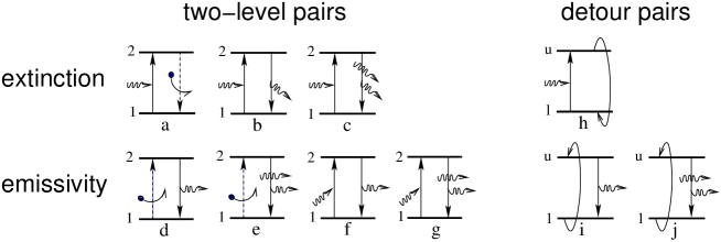
Figure 1.: Atomic transitions governing line formation arranged in photon-involving pairs. The beam of interest (direction of the intensity vector) is to the right. Detour paths (schematic in pairs h, i, j; see Figure fig:detours) combine transitions involving other levels and may include analogous bound–free transitions. The upper row shows pair combinations contributing line extinction: collisional photon destruction (a), scattering out of the beam (b and c), photon conversion out of the beam (h, into other-wavelength photons and/or kinetic energy). The lower row shows pairs contributing line emissivity: collisional photon creation (d and e), scattering into the beam (f and g), detour photon production into the beam (i and j). Pairs c and g have equal probability by requiring one photon in the beam and one with arbitrary direction. From SSF, extension of RTSA Figure 3.3. fig:pairs

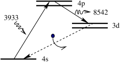
Figure 2.: Detour examples. Left: Ca ii 8542 Å emission in a bound-bound “interlocking” detour loop: $3d$–$4s$ down per collision (forbidden transition) followed by $4s$–$4p$ Ca ii  K photo-excitation up and $4p$–$3d$ photo-deexcitation down back to the $3d$ level, adding a Ca ii 8542 Å photon to the beam. Starting at the $4s$ Ca ii ground level the loop back to it extincts a Ca ii  K photon by conversion into a Ca ii 8542 Å photon plus kinetic energy. Right: H $\alpha$ emission in a bound–free detour loop: photo-ionization from H i $n\!=\!\!\,2$ by the Balmer continuum followed by photo-recombination into a Rydberg level and downward cascade with $\Delta n\!=\!\!\,1$ steps, first as collisional deexcitations and then as photo-deexcitations ending by adding an H $\alpha$ photon to the beam. The extincted Balmer-continuum photon is converted into longer-wavelength photons plus kinetic energy. fig:detours

2 Equilibria

sec:equilibria

Figure fig:pairs is a pairwise inventory of the five Einstein bound–bound processes affecting photons (RTSA Section 2.3.1): photo-excitation (at left in pair a), spontaneous photo-deexcitation (at right in pair b), induced photo-deexcitation (in pair c), collisional excitation (in pair d), and collisional deexcitation (in pair a). The pairs at left describe two-level-only combinations; the pairs at right multi-level detours where “detour” represents the sum of all possible indirect transition paths from the upper level to the lower level or vice versa; common cases are shown in Figure fig:detours. The diagrams in Figure fig:pairs can be drawn similarly for bound–free ionization/recombination transitions.

Assuming statistical equilibrium (SE, constant level populations with time) gives two extreme equilibria: LTE when collisional pairs a, d, and e dominate, coronal equilibrium (CE) when pair d dominates exclusively.

LTE requires sufficiently high density that most excited atoms already deexcite per collision before doing so radiatively (spontaneous or induced) within their excited-state lifetime. LTE is valid throughout the Sun up to its surface. Because LTE requires colliders both up and down the corresponding Boltzmann upper-to-lower level, population ratios within an ionization stage depend only on temperature. Saha upper-to-lower ion stage population ratios depend additionally on the electron density because, in addition to LTE-enforcing colliders both for ionization and recombination, another electron needs to be caught for recombination.

CE requires sufficiently low gas and radiation densities that every collisional excitation (ionization) is followed by spontaneous deexcitation (photorecombination). CE is valid for most EUV lines from the corona. The stage ratios then depend only on temperature, the level ratios also on collider (electron) density.

NLTE describes SE situations between these two extremes. The name is a misnomer, meaning assuming SE without assuming LTE. It may encompass the above extremes: for example, LTE is reached at the bottom of the NLTE VALIIIC atmosphere of Vernazza, Avrett, and Loeser (1981), CE at its top. “NLTE departures” mean population differences with Saha–Boltzmann values, source function differences with the Planck function.

An additional NLTE complexity is the issue whether in resonance scattering (pairs f, g) the new beam photon “remembers” the precise wavelength of the exciting photon (p. 2 of Eddington, 1929). In coherent scattering it has the same wavelength, in complete redistribution (CRD) it resamples the profile. Partial frequency redistribution (PRD) evaluates coherent scattering with Doppler redistribution and collisional redistribution at high collider density. Doppler redistribution occurs always because even when atoms scatter coherently in their own frame the observer sees an ensemble sampling different particle motions. In the case of systematic motions the line source function becomes anisotropic and angle redistribution must also be accounted for. For most solar lines CRD is a sound assumption (generally made since Houtgast, 1942) but Ca ii H & K, Mg ii h & k, Ly$\hskip 0.86108pt\alpha$, and other strong ultraviolet lines with high-up core formation at low density require PRD modeling.

Bound-free transitions are not intrinsically different from bound–bound transitions (the rate descriptions can be unified, see RTSA Section 3.2.3); they differ only in the larger extent and threshold cutoff of their profile function and in obeying complete redistribution over that since the electron caught for recombination samples the Maxwell distribution without memory.

Non-E is the non-SE generalization of NLTE to time-dependent populations. Non-E can be important in situations where gas cools after being heated because the settling speed to collisional equilibrium has near-Boltzmann temperature sensitivity from the Einstein relation between collisional up- and down rates (RTSA Eqs. 3.32 and 3.33). Settling slow-down in cooling gas is most important in the large H i Ly$\hskip 0.86108pt\alpha$ jump and causes retarded hydrogen recombination discussed further in Section sec:nonEmm. Non-E is likely also important in ionization/recombination settling of other species with high $n\!=\!\!\,2$ excitation energy including He i  (Golding, Carlsson, and Leenaarts, 2014), Si iii and O iii (Nóbrega-Siverio, Moreno-Insertis, and Martínez-Sykora, 2018).

With “non-equilibrium spectrum formation” in the title I mean relaxing LTE into NLTE for the formation of both lines and continua, discarding the assumption of static magnetism-free hydrostatic equilibrium by using dynamical MHD simulations, and replacing SE by non-E where necessary both in simulations and in spectral synthesis.

Figure 3.: Schematic optically thick solar line formation. The line extinction $\alpha^{l}$ diminishes with height with density, likely also with temperature (Boltzmann excitation), increasing ionization, and more. In the absence of systematic motions its extinction profile is symmetric around line center. It has damping wings at lower height (h1) from larger collider density, while its Doppler core narrows with height (from lower temperature and/or less microturbulence). The total extinction (upper left) is its sum with the local continuum extinction $\alpha^{c}_{\lambda}$, which is typically orders of magnitude less (Figure fig:extinction), hence the logarithmic scale. Summation of $\alpha_{\lambda}^{\rm total}$ against height delivers the optical depth scaling (upper right) which is usually roughly linear in $\log\tau(h)$ due to hydrostatic exponential density decay. The $\tau\!=\!\!\,1$ locations define where to sample the total source function $S_{\lambda}$ to obtain the emergent intensity in Eddington–Barbier fashion (lower row). $S_{\lambda}$ is the extinction-weighted combination of $S_{\lambda}^{\rm line}$ and $S_{\lambda}^{\rm cont}$. The emergent line $I_{\lambda}\!\approx\!\!\,S_{\lambda}(\tau_{\lambda}\!=\!\!\,1)$ is in absorption because $S_{\lambda}$ drops; for an optically thick emission line $S_{\lambda}$ must increase with height. This schematic mimics the formation of the solar Na i D lines in Figure 4 of Uitenbroek and Bruls (1992) by having $S_{\lambda}^{\rm cont}\!\approx\!\!\,B_{\lambda}$ with a temperature minimum and a $\sqrt{\varepsilon}$-like scattering drop in $S_{\lambda}^{\rm line}$. In LTE the line would show a core reversal. This quartet may be similarly drawn for bound–free transitions, with as major change the wide spectral extent and non-symmetric triangular shape of the extinction edge in the first panel. In the lower-right panel it is then more realistic to draw $S_{\lambda}^{\rm edge}$ as less steeply decaying than $B_{\lambda}$ and without outer rise, as in Figure fig:schemscat. From SSF. fig:4panel

3 Spectrum Formation in a Nutshell

sec:equations

This section is a brief summary of radiative transfer in stellar atmospheres, with key equations. It refers much to RTSA, with page openers. The bibles of the field are Mihalas (1970, 1978) and Hubený and Mihalas (2014). Good summaries of numerical approaches are given by Werner et al. (2003) and Pereira (2019).

Figure fig:4panel illustrates optically thick solar spectrum formation using the Eddington–Barbier approximation

$$I_{\lambda}(0,\mu)\approx S_{\lambda}(\tau_{\lambda\mu}\!=\!\!\,1)\mbox{~{}~{}~{}or~{}~{}~{}}I_{\lambda}(0,\mu)\approx S_{\lambda}(\tau_{\lambda}\!=\!\!\,\mu)\ilabel{eq:EB}$$ (1)

for the monochromatic emergent intensity $I_{\lambda}(0,\mu)$ in direction $\mu\!\equiv\!\cos\theta$, with $\theta$ the viewing angle between line of sight and local vertical and $S_{\lambda}$ the total source function. The optical depth $\tau_{\lambda\mu}$ is measured inwards by summing the extinction per cm $\alpha_{\lambda}$ along the line of sight with $\tau\!=\!\!\,0$ the mathematical outer surface (in your telescope), whereas the more common $\tau_{\lambda}(h_{0})\!\equiv\!-\int_{\infty}^{h_{0}}\alpha_{\lambda}\>{\rm d}h$ is the radial optical depth for axial symmetry (plane-parallel layers).

This relation is obtained by linearizing the Laplace transform of the source function (RTSA p. 86), which is the solution of the integral form of the intensity transfer equation in an outward direction at the surface of a non-irradiated star (RTSA Eq. 4.10). Although this is only an approximation and can go wrong, it says that one should inspect the source function where the summed extinction reaches unity, the observational “surface”. The latter says where one looks, the former what one may see. This recipe holds alike for solar observations, 1D modeling, and numerical simulations.

The recipe does not hold for optically thin features (e.g. filaments) for which one instead quantifies total emissivity $j_{\lambda}$ along the line of sight, requiring problematic accounting for irradiation from below and sideways unless radiation-free CE can be assumed as is done for coronal EUV lines.

Thus, for photospheric and chromospheric radiation one evaluates the extinction for “where” and the source function for “what”. These quantities are more orthogonal than extinction and emissivity: to first order the extinction describes the local density of the particular particles that contribute extinction at a specific wavelength whereas the source function describes the local environment (gas density, temperature and impinging radiation) governing what happens after extinction (photon destruction, scattering, or conversion in Figure fig:pairs). In LTE this orthogonality is perfect: $\alpha_{\lambda}$ and $j_{\lambda}$ then share the same bound–bound spike while $S_{\lambda}\!=\!\!\,B_{\lambda}$ with $B_{\lambda}$ the Planck function, which is smooth across a line ignoring its existence. However, this split between where and what can get mixed: for example in much of the solar atmosphere the extinction in H $\alpha$ (“where”) is set by radiation in Ly$\hskip 0.86108pt\alpha$ with its own “what” conditioning.

Equation eq:EB is for total extinction and total source function. Continuous and line extinctions add up directly being cross-sections ($\alpha_{\lambda}$ per cm may be seen as volume coefficient with cross-section cm² per cm³), with the caveat that the emissivity from induced deexcitations be counted as negative extinction to accommodate the mutual cancelation of pairs c and g in Figure fig:pairs. The total source function (emissivity divided by extinction; the word source implies addition of new photons into the beam) is the weighted mean over all contributing processes $S_{\lambda}^{\rm tot}=\sum j_{\lambda}/\sum\alpha_{\lambda}$, in particular $S_{\lambda}^{\rm tot}=(j^{c}_{\lambda}+j^{l}_{\lambda})/(\alpha^{c}_{\lambda}+\alpha^{l}_{\lambda})=(S_{\lambda}^{c}+\eta_{\lambda}S_{\lambda}^{l})/(1+\eta_{\lambda})$ where this $\eta_{\lambda}$ is the line strength $\alpha_{\lambda}^{l}/\alpha_{\lambda}^{c}$ and $S_{\lambda}^{\rm tot}$ is always frequency-dependent across a line even when $S_{\lambda}^{l}$ is not by obeying CRD.

Since both the line source function and the line extinction depend on the lower- and upper-level population densities we employ shorthand NLTE departure coefficients (RTSA Section 2.6.2):

$$b_{l}=n_{l}/n^{\rm LTE}_{l}\mbox{~{}~{}~{}~{}~{}~{}~{}~{}}b_{u}=n_{u}/n^{\rm LTE}_{u},\ilabel{eq:zwaan}$$ (2)

where $n^{\rm LTE}$ is the population density of the level computed per Saha–Boltzmann from the total element density $N_{\rm elem}$. The general line extinction coefficient so becomes (RTSA Eq. 2.111, RTSA Eq. 9.6):

$$\alpha^{l}_{\lambda}=\frac{\pi e^{2}}{m_{\rm e}c}\,\frac{\lambda^{2}}{c}\,b_{l}\,\frac{n_{l}^{\rm LTE}}{N_{\rm elem}}\,N_{\rm H}\,A_{\rm elem}\,f_{lu}\,\varphi\left[1-\frac{b_{u}}{b_{l}}\,\frac{\chi}{\varphi}\,\>{\rm e}^{-hc/\lambda kT}\right],\ilabel{eq:genalpha}$$ (3)

where $A_{\rm elem}$ is the relative element abundance with $N_{\rm elem}\!=\!\!\,A_{\rm elem}N_{\rm H}$, $f_{lu}$ is the oscillator strength, and $\chi$ and $\varphi$ are the area-normalized profile functions for induced emission and extinction.

The general line source function is (RTSA Eq. 2.105):

$$S_{\lambda}^{l}=\frac{2hc^{2}}{\lambda^{5}}\frac{\psi/\varphi}{\displaystyle\frac{b_{l}}{b_{u}}\>{\rm e}^{hc/\lambda kT}-\frac{\chi}{\varphi}}\ilabel{eq:genS}$$ (4)

with $\psi$ the spontaneous emission profile. For CRD $\psi=\chi=\varphi$ so that the profile ratios simplify to unity. In the Wien approximation, generally valid throughout the optical and ultraviolet (H $\alpha$ reaches $\lambda T\!=\!\!\,hc/k$ at 21 900 K), the CRD expressions simplify further to:

$$\alpha_{\lambda}^{l} \approx b_{l}\,\,\alpha_{\lambda}^{\rm LTE}$$ (5)

$$S_{\lambda}^{l} \approx (b_{u}/b_{l})\,\,B_{\lambda}(T),$$ (6)

which are the quick NLTE recipes for “where” and “what”: line extinction scales with $b_{l}$, the line source function with $b_{u}/b_{l}$. The latter gives $S_{\lambda}^{l}\!=\!\!\,B_{\lambda}$ for $b_{u}\!=\!\!\,b_{l}$; this is not the definition of LTE but a corollary: LTE is defined as Saha–Boltzmann partitioning with $b_{u}\!=\!\!\,b_{l}\!=\!\!\,1$ (Section 1.4 of Ivanov, 1973).

Equation eq:WienS quantifies NLTE departure from the Planck function but not how it comes about. This needs splitting the line extinction coefficient into the destruction (a for absorption), scattering (s), and detour (d) contributions of Figure fig:pairs:

$$\alpha_{\lambda}^{l}\equiv\alpha_{\lambda}^{\rm a}+\alpha_{\lambda}^{\rm s}+\alpha_{\lambda}^{\rm d}\hskip 28.45274pt\varepsilon_{\lambda}\equiv\alpha_{\lambda}^{\rm a}/\alpha_{\lambda}^{l}\hskip 28.45274pt\eta_{\lambda}\equiv\alpha_{\lambda}^{\rm d}/\alpha_{\lambda}^{l}\ilabel{eq:epseta}$$ (7)

where $\varepsilon$ is the collisional destruction probability of an extincted photon and $\eta$ is its detour conversion probability. With these the general line source function becomes either

$$S_{\lambda}^{l}=(1-\varepsilon_{\lambda}-\eta_{\lambda})\,J_{\lambda}~{}+~{}\varepsilon_{\lambda}B_{\lambda}(T)~{}+~{}\eta_{\lambda}S_{\lambda}^{\rm d}\ilabel{eq:S_{C}S}$$ (8)

or

$$S_{\lambda_{0}}^{l}=(1-\varepsilon_{\lambda_{0}}-\eta_{\lambda_{0}})\,\overline{J_{\lambda_{0}}}~{}+~{}\varepsilon_{\lambda_{0}}B_{\lambda_{0}}(T)~{}+~{}\eta_{\lambda_{0}}S_{\lambda_{0}}^{\rm d}.\ilabel{eq:S_{C}RD}$$ (9)

The first version is for coherent (monofrequent, monochromatic) scattering. The second is for CRD with $\overline{J_{\lambda_{0}}}\equiv(1/4\pi)\int\!\!\int I_{\lambda}\varphi(\lambda\!-\!\lambda_{0})\>{\rm d}\lambda\>{\rm d}\Omega$ the “mean mean” intensity averaged over all directions and the line profile, with $\lambda_{0}$ the line-center wavelength and also used as line identifier. The first term in Eqs. eq:S_CS and eq:S_CRD represents the reservoir of photons that contribute scattering, the second describes collisional photon creation, the third the contribution of new line photons via detours. The LTE $S\!=\!\!\,B$ equality holds when $\varepsilon\!=\!\!\,1,\eta\!=\!\!\,0$ and/or $J\!=\!\!\,S^{\rm d}\!=\!\!\,B$, both true below the standard $h\!=\!\!\,0$ surface at $\tau_{5000}^{c}\!=\!\!\,1$. Above it $\varepsilon$ becomes small from lower electron density while $\eta$ is usually smaller; all bound–bound lines and bound–free continua formed above a few hundred km height are heavily scattering with $S\!\approx\!\!\,J$ (but free–free continua always have $S\!=\!\!\,B$ because each interaction is collisional).

H $\alpha$ has a sizable $\eta S^{\rm d}$ contribution from detour loops as in Figure fig:detours. This was famously called “photoelectric control” by Thomas (1957) but wrongly because even this complex line is mostly scattering, although with unusual backscattering from chromosphere to photosphere (Rutten and Uitenbroek, 2012).

The final and most important equation is the Schwarzschild equation (page 361 of Hubený and Mihalas, 2014; RTSA Eq. 4.14):

$$J_{\lambda}(\tau_{\lambda})=\frac{1}{2}\int_{0}^{\infty}S_{\lambda}(t_{\lambda})\,E_{1}(|t_{\lambda}\!-\!\tau_{\lambda}|)\>{\rm d}t_{\lambda}\equiv\hbox{$\bf\Lambda$}_{\tau_{\lambda}}[S_{\lambda}(t_{\lambda})]\ilabel{eq:lambdop}$$ (10)

with exponential integral $E_{1}(x)=\int_{0}^{1}\>{\rm e}^{-x/\mu}\,{\rm d}\mu/\mu$ (RTSA Eq. 4.12). Its weighting of the source function makes the kernel of the $\bf\Lambda$ operator very wide. The cutoff at the surface produces outward $J_{\lambda}(\tau_{\lambda})<S_{\lambda}(\tau_{\lambda})$ divergence for small inward increase of $S_{\lambda}(\tau_{\lambda})$ but outward $J_{\lambda}(\tau_{\lambda})>S_{\lambda}(\tau_{\lambda})$ divergence for steep increase (RTSA Figure 4.2, RTSA Figure 4.4 from Kourganoff, 1952, RTSA Figure 4.9). Be aware that steep horizontal gradients are similarly important in 3D radiative transfer as the radial ones entering $\bf\Lambda$ in plane-parallel Eq. eq:lambdop. Steep horizontal gradients occur in and above granulation and also in and around the MCs that make up network and plage and so affect their irradiance contributions.

Equation eq:lambdop defined the industry of “approximate/accelerated lambda iteration” (RTSA Section 5.3.2) following the operator splitting of Cannon (1973). The need for iteration when simplistic LTE can not be assumed is obvious from comparing Eqs. eq:S_CRD and eq:lambdop: determining $S$ for using Eq. eq:EB needs $J$ and that requires $S$ over a range of depths. Thus, the observed intensity depends non-locally on radiation from elsewhere, not only for the source function for “what” but also for the extinction for “where” when that senses radiation (as in the extinction of H $\alpha$ controlled by radiation in Ly$\hskip 0.86108pt\alpha$). With overlapping transitions (the local continuum for starters) and interlocking (the multi-level $\eta$-term) this involves all pertinent transitions connected one way or other to the one of interest. This quickly grows into having to solve radiative transfer and associated atomic-level population equations for many species at many wavelengths in multiple directions throughout the atmosphere. Solar spectrum modeling so developed into a computational resource-limited endeavor with clever code development of principal importance.

At its very start Avrett (1965) computed his canonical demonstration (RTSA Figure 4.12) of the quintessential $\sqrt{\varepsilon}$ law: in a two-level-atom isothermal atmosphere with constant $\varepsilon$ the line source function drops outward to $S^{l}=\sqrt{\varepsilon}\,B$ at the $\tau\!=\!\!0$ physical surface, both for coherent scattering and CRD. The emergent intensity ($\!\approx\!\!\,S$ at the $\tau\!=\!\!\,1$ observed surface) is nearly as small. The thermalization depth where $J$ starts dropping below $B$ due to scattering photon losses lies as deep as $1/\varepsilon$ in line-center optical depth units, even deeper in the presence of damping wings permitting long photon steps (RTSA Section 4.3 and Avrett’s lecture notes). The upshot is that scattering lines get very dark, as the Na i D lines in Figure fig:haze with their formation sketched in Figure fig:4panel. A simple explanation is given in Section 1.7 of Rybicki and Lightman (1986), an elaborate one in Hubený (1987).

Figure 4.: Scattering in the solar atmosphere. Left: continua. Right: lines. $B$ (solid) and $J$ (dashed) are shown as temperature to have the same scales at different wavelengths. The $B$ curve mimics the solar atmosphere in having a radiative-equilibrium decline, a higher-temperature chromosphere, and a steep increase to coronal values. From SSF. fig:schemscat

4 Scattering Overview

sec:schemscat Figure fig:schemscat sketches the behavior of $B$ and $J$ in continua and lines as electron temperature and radiation temperature. Temperature representation (with excitation temperature for $S$, see RTSA p. 37 ff.) enables direct comparison between different wavelengths by undoing Planck-function temperature sensitivities.

The first sketch in Figure fig:schemscat shows continua with $J>B$ in the ultraviolet but $J\!\approx\!\!\,B$ in the optical and $J<B$ in the infrared. The physical reason is that the upper photosphere (above the granulation and below the heights where acoustic waves shock and MCs expand into canopies, still predominantly neutral) is the most homogeneous domain of the solar atmosphere, fine-structured primarily by non-shocking acoustic and gravity waves, and generally close to radiative equilibrium. This condition requires a temperature decline producing spectrum-integrated $\alpha S\!\approx\!\!\,\alpha J$ (RTSA Section 7.3.2). The bulk of the solar radiation escapes in the optical and so imposes $S\!\approx\!\!\,J$ in this part of the spectrum. The optical continuum has $S\!\approx\!\!\,B$ thanks to H${}^{{}^{{}_{-}}}$ dominance, so that its radiative equilibrium sets the upper-photosphere temperature decline.

With this imposed decline $\bf\Lambda$ produces $J>B$ divergence in the ultraviolet. This holds already in LTE from the nonlinear Wien sensitivity (RTSA Figure 4.9): the optical $S\!\approx\!\!\,B$ transforms into $J>B$ using $\bf\Lambda$ in the ultraviolet because $B(h)$ is much steeper there. Yet larger $J>B$ divergence results from NLTE bound–free scattering because the effective photon escape depths then lie deeper than $\tau\!\approx\!\!\,1$, sampling yet steeper temperature increase in the deep photosphere. The ultraviolet photons that are collisionally created there scatter outward gaining $J>B$ because the actual $B(h)$ gradient is steeper than what they would themselves impose for equilibrium. Eventually $J$ flattens to constancy (out to infinite height above infinite-extent plane-parallel models). In the chromosphere the independent non-equilibrium temperature rise results in $J<B$ above this limit value. These ultraviolet $J\neq B$ patterns produce corresponding $S\neq B$ departures where scattering dominates.

The infrared and mm regions have $J<B$ from $\bf\Lambda$ (RTSA Figure 4.9) but this has no effect on $S$ since $S\!=\!\!B$ for the scatter-free H${}^{{}^{{}_{-}}}$ and H i free–free processes.

The right-hand sketch in Figure fig:schemscat depicts scattering lines with increasing extinction. The decoupling of $J$ from $B$ occurs higher for stronger lines. $J$ drops below $S$ qualitatively following the isothermal $\sqrt{\varepsilon}$ law, also in the radiative-equilibrium decline because at large line extinction the $\tau$ scale gets compressed so that $B(\tau)$ drops less steeply than in the continuum (RTSA Figure 4.10).

This sketch also represents a schematic for the formation of PRD lines. Their core, inner-wing, and outer-wing parts represent independent radiation ensembles, each scattering out on its own with its own decoupling height and decay from $B$. Across a strong line the rightmost $J$ curve describes line-center scattering, the ones more to the left scattering further away from line center with deeper decoupling.

Figure 5.: The FALC quiet-Sun model of Fontenla, Avrett, and Loeser (1993). The electron density $N_{\rm e}$ (dashed) has $10^{-4}$ offset from the hydrostatically decaying total hydrogen density $N_{\rm H}$ (solid) over $h\!=\!\!\,100-700$ km. Below and above this range hydrogen has partial ionization above $10^{-4}$, reaching full ionization below 0 km and above 2100 km. Above 1500 km ionization makes the neutral hydrogen density $N_{{\rm H}{\rm I}}$ (dotted) drop below $N_{\rm H}$. After SSX. fig:FALC

5 FALC Demonstrations

sec:demonstrations

This section illustrates solar spectrum formation using examples for a standard 1D model atmosphere to illustrate NLTE effects that affect solar irradiance. The graphs were made with the RH spectral synthesis code of Uitenbroek (2001) for the FALC model of Fontenla, Avrett, and Loeser (1993).

RH does not iterate $\bf\Lambda$ but the emissivity $\Psi$ operator of Rybicki and Hummer (1992). It permits overlapping lines, it includes PRD and full-Stokes options, it exists in 1D, 2D, 3D, spherical, and Cartesian versions, and more recently also in parallel multi-column “1.5D” (Pereira and Uitenbroek, 2015). Here its 1D version-2 is used with H, He, Si, Al, Mg, Fe, Ca, Na, and Ba active, C, N, O, S, and Ni passive, and with 20 mÅ sampling of 343 000 lines between 1000 and 8000 Å in the atomic and molecular line list of Kurucz (2009).

FALC, shown in Figure fig:FALC, is the average-quiet-Sun companion of the FALP plage model at the basis of the SATIRE irradiance modeling. It is therefore used here rather than Avrett’s latest quiet-Sun model (ALC7 of Avrett and Loeser, 2008). Their differences are compared in SSX but are not significant for the demonstrations here.

While well-known and often-cited, these 1D modeling efforts do not describe the actual solar atmosphere realistically. Even if its fine structures were just temperature fluctuations around a well-defined mean temperature stratification, then the latter is not retrieved by fitting the mean-intensity spectrum in the optical and ultraviolet due to non-linear Wien weighting, as shown for acoustic shocks by Carlsson and Stein (1995) and for granulation by Uitenbroek and Criscuoli (2011). The 1D models should be regarded as hypothetical plane-parallel stars with a spectrum remarkably mimicking the solar spectrum that are useful to demonstrate spectrum formation governed by the equations above (RTSA p. 189). In RTSA I added didactic demonstrations from the monumental VALIII modeling of Vernazza, Avrett, and Loeser (1981) and its informative graphs (e.g. RTSA Figures 8.9 ff. from the 11-page Figure 36). Here I add demonstrations with FALC and RH-output plotting programs on my website.

Figure 6.: Extinction in the FALC star at heights 0, 500, 1000, 1500, and 2000 km from top to bottom. The top curve for $h\!=\!\!\,0$ km is for total extinction: continuous plus all lines in the RH setup from active and passive atoms and the Kurucz-list sampling over 1000 – 8000 Å. The other curves are for continuous extinction only. The line haze is densest in the ultraviolet and violet. At larger height the ultraviolet edges are replaced by Rayleigh scattering off neutral and excited hydrogen atoms with $\propto\!\lambda^{-4}$ decreases, the optical H${}^{{}^{{}_{-}}}$ bf bulge below 1.6 $\mu$m ($\log\,\lambda[{\rm\AA}]\!=\!\!\,4.2$) by Thomson scattering off free electrons without wavelength variation, and the H${}^{{}^{{}_{-}}}$ ff increase above 1.6 $\mu$m by H i ff extinction of protons with $\propto\!\lambda^{2}$ increase. At $\log\alpha_{\lambda}\!=\!\!\,-7$ a 100-km thick feature becomes optically thick (cf. Figure fig:extsb). Towards shorter and longer wavelengths one observes higher in the FALC atmosphere, with $\tau_{\lambda}\!=\!\!\,1$ sampling of the chromosphere reached below $\lambda\!\approx\!\!\,1600$ Å ($\log\,\lambda[{\rm\AA}]\!=\!\!\,3.2$) and above $\lambda\!\approx\!\!\,160\,\mu$m ($\log\,\lambda[{\rm\AA}]\!=\!\!\,6.2$) (cf. Figure 1 of Avrett, 1990). fig:extinction

5.1 FALC Extinction

sec:extinction

Figure fig:extinction is an overview of FALC extinction. Because FALC is a solar-like high-metallicity star, ionization of the electron donors (abundant elements with low first ionization threshold: Si i, Fe i, Al i, and Mg i, see RTSA Figure 7.1) produces $N_{\rm e}\!\approx\!\!\,10^{-4}\,N_{\rm H}$ throughout the photosphere, enough to make it opaque through combining with H into H${}^{{}^{{}_{-}}}$. At mm wavelengths H${}^{{}^{{}_{-}}}$ free–free extinction is replaced by H i free–free extinction when the $\tau_{\lambda}\!=\!\!\,1$ height reaches hydrogen ionization. These free–free processes strictly obey source function $S\!=\!\!\,B$ equality. The H${}^{{}^{{}_{-}}}$ bound–free part governing the optical continua does not share this virtue, but because the H${}^{{}^{{}_{-}}}$ ionization energy is less than the average kinetic energy $S\!\approx\!\!\,B$ is usually valid up to the heights were Thomson scattering takes over. In contrast, the Balmer and metal edges that together supply increasing extinction below 3700 Å are heavily scattering. Since the neutral metals producing them also produce most lines in the ultraviolet and optical (in particular Fe i), these are all affected by this bound–free scattering as shown below.

Figure 7.: Ultraviolet continua in the FALC star. Left: departure coefficients $b_{1}$ and $b_{c}$ for the neutral (solid) and ion (dashed, all near unity) ground states of the major bound–free opacity providers Si, Fe, Al, and Mg. For hydrogen the solid line near unity shows $b_{2}$ for $n\!=\!\!\,2$, the dashed curve $b_{c}$ for the proton density. Right: $B$ (solid), $S$ (dotted), $J$ (dashed) averaged over 100 Å wide bands around the specified wavelengths including all Kurucz lines, for the atomic ones using the two-level scattering approximation (Section sec:linehaze). $S$, $B$ and $J$ are plotted as formal temperatures to obtain equal scales at different wavelengths. The ticks on each $S$ curve are at $\tau\!=\!\!\,3,1,0.3$ for 1500 Å, for $\tau\!=\!\!\,1$ and 0.3 for 3500 Å and 2500 Å (the latter around $h\!=\!\!\,100$ km) for which the $\tau\!=\!\!\,3$ values lie below $h\!=\!\!\,0$ km near 7500 K outside the frame. At 2500 Å the latter lies so deep due to Mg i ionization (VALIII Figure 36). After SSX. fig:edges

5.2 FALC Ultraviolet Continua

sec:uvcontinua

The ultraviolet continua from the Balmer threshold at 3646 Å down to the Lyman threshold at 912 Å form at increasing height by the summed extinction of the bound–free edges of Mg i, Al i, Si i, Fe i, and C i superposed on the Balmer edge (Figure fig:extinction, specification in VALIII Table 9).

Figure fig:edges samples their FALC formation. At left it shows representative population departures, at right continuum formation at three representative wavelengths. The $\tau$ marks show that at 3500 Å the continuum has final photon escape in the deep FALC photosphere, at 2500 Å in the low photosphere, at 1500 Å in the onset of the FALC temperature rise. However, the effective onset of scattering radiation escape (thermalization depth) is in the deep photosphere for all three continua as shown by their $J>B$ divergence. Assuming $S\!=\!\!\,B$ as in SATIRE underestimates their intensities and overestimates their limb darkening. Above the FALC temperature minimum the $B$ increase is not followed by the flattening $J$ curves. The $S$ curves sense $B$ somewhat but only above $\tau_{\lambda}\!=\!\!\,1$.

This photospheric control occurs similarly for ultraviolet continua computed with the 1D FALP model, with network and plage brightening in the ultraviolet from the higher deep-photosphere temperatures. Model-imposed ultraviolet MC brightening also holds for its SATIRE modification which has no chromosphere and uses $S\!=\!\!\,B$ contrast rather than NLTE-derived $S\!\approx\!\!\,J$ contrast to mimic actual multi-D deep-hole radiation.

The scattering $S-B$ splits at right translate with Eq. eq:WienS into $b_{c}/b_{l}$ ratios shown at left as logarithmic divergences. The metals are mostly ionized with most of the element in the ion ground state so that $b_{c}\!\approx\!\!\,1$ (dashed) whereas the minority $b_{1}$ curves (solid) have substantial dips from radiative over-ionization and steep rises higher up from radiative under-ionization. The corollary is that all lines of these species, in particular all Fe i lines, have significant opacity depletion with respect to LTE which starts already in the deep photosphere. For the strongest lines it reverses into large over-opacity in the FALC chromosphere.

The ionization of hydrogen is mostly from level $n\!=\!\!\,2$ so that the Balmer continuum pattern at right defines FALC hydrogen ionization departures. Hydrogen is virtually neutral below the FALC transition region so that $b_{1}\!\approx\!\!\,1$, and also Ly$\hskip 0.86108pt\alpha$ is virtually in detailed balance so that $b_{2}\!\approx\!\!\,b_{1}\!\approx\!\!\,1$ (solid), giving LTE extinction to the Balmer lines and continuum. Therefore $b_{c}$ (dashed) shows the Balmer over- and under-ionization pattern reversely to $b_{1}$ of the metals.

A warning: Figure fig:edges demonstrates scattering from radial temperature gradients. In the actual time-dependent 3D solar atmosphere comparable ultraviolet $S-B$ scattering divergences occur for fine-structure gradients such as the steep outward and lateral ones around granules, across hot walls in MCs, and around small-scale heating events. Any treatment short of detailed 3D$(t)$ radiative transfer is an approximation.

Figure 8.: Fe i 6302 Å in the FALC star. Left: $b_{u}$ and $b_{l}$ (solid). Dashed: population fraction $n_{l}/N_{\rm elem}$ (axis at right). Dotted: same in LTE (Saha–Boltzmann fraction). Right: corresponding $B$ (thin solid), $J$ (dashed), and $S$ (thick solid) as formal temperatures. Dotted: two-level collisional destruction probability $\varepsilon_{2}=C_{ul}/(C_{ul}+A_{ul}+B_{ul}B)$ (scale at right). Dot-dashed: two-level thermalization length $\Lambda_{2}=\sqrt{\pi}/(\alpha_{\lambda_{0}}\varepsilon_{2})$ for the Doppler core in gigameters (scale at right). Example: $\log\Lambda_{2}\!=\!\!\,-6$ implies thermalization of $S$ to $B$ at the center of a two-km thick feature. The curve label is placed besides the curve at the line-core thermalization height. The numbered ticks in both panels specify $\log\tau$ heights for line center. After SSX which offers such graphs for many lines and multiple standard models. fig:Fe6302

Figure 9.: Fe i 3860 Å in the FALC star. Format as Figure fig:Fe6302. fig:Fe3860

5.3 FALC Iron Lines

sec:lines

Since irradiance studies are more concerned with the multitude of spectral lines than with the specific lines employed in resolved solar physics, the champion line producer is sampled here by showing FALC formation for two Fe i lines, a weak optical one and a strong near-ultraviolet one.

Figure fig:Fe6302 is for the well-known optical polarimetry line at 6302 Å. The curve for two-level $\varepsilon_{2}=C_{ul}/(C_{ul}+A_{ul}+B_{ul}B)$ in the right-hand panel follows the electron density in Figure fig:FALC and drops to $10^{-2}$ near $\tau\!=\!\!\,1$, suggesting domination by scattering in Eq. eq:S_CS. Thermalization occurs near $\tau\!=\!\!\,10$ in the deep photosphere, but $S$ departs from $B$ only above $\tau\!=\!\!\,1$ to follow $J$ more closely. The reason for this apparent discrepancy is multi-level interlocking (the $\eta$ terms in Eq. eq:S_CS) from the richness of the Fe i Grotrian diagram. This line is a fairly high-lying (multiplet 816, 3.6 – 5.6 eV) subordinate one among many others, as are most optical Fe i lines. Their levels are connected to lower levels by much stronger lines, mostly in the ultraviolet, that de-thermalize ($S\!\approx\!\!\,J$ uncoupling from $B$) further out and so force $b_{u}\!=\!\!\,b_{l}$ equality for their weaker siblings. Likewise, many weaker Fe i lines are members of multiplets in which the strongest members impose similar thermalization. The upshot is that most weak Fe i lines have source function LTE (“what”) thanks to the rich term structure.

However, they do not have extinction LTE (“where”). This is evident from the $b_{l}$ curve in the left-hand panel which follows the ultraviolet-imposed pattern of photospheric dip and chromospheric rise in Figure fig:edges. It translates into the divergence between the LTE and NLTE fraction curves, whereas the $b_{l}\!-\!b_{u}$ split corresponds to the NLTE $B\!-\!S$ split at right (Eqs. eq:Wienalpha and eq:WienS). Polarimetry “inversions” with this line and/or similar ones often obtain NLTE source function estimates from best-fit modeling but ignore the more important $b_{l}$ dip in the extinction.

Figure fig:Fe3860 is in the same format but for a strong near-ultraviolet Fe i line, member of multiplet 4 from the ground state. The latter has fractional population (dashed curve at left) about $10^{-2}$ or less, confirming that iron is predominantly ionized everywhere. The Saha–Boltzmann value (dotted) is significantly higher in the photosphere and lower in the FALC chromosphere because the $b_{l}$ curve is the $b_{1}$ curve of Figure fig:edges set by ultraviolet bound–free scattering. The $b_{u}$ curve drops away from it following the $B\!-\!S$ split at right. This line scatters more strongly ($\varepsilon_{2}$ below $10^{-3}$) and behaves more as a two-level line, with thermalization near $\tau\!=\!\!\,10^{3}$ and $S\!\approx\!\!\,J$ separation from $B$ starting already there, far below its $\tau\!=\!\!\,1$ height, and with only marginal sensitivity to the FALC temperature rise so that the emergent profile is an absorption dip without core reversal. One might call the line “chromospheric” because it has $\tau\!=\!\!\,1$ above $h\!=\!\!\,1000$ km, but its core intensity responds rather to temperature modulation of the FALC temperature minimum where the emerging photons are created. However, line-core Doppler and Zeeman measures are imposed at the last scattering and do respond higher up.

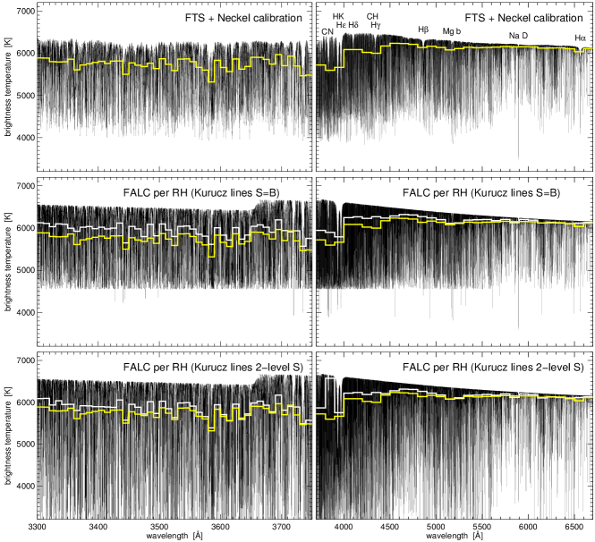
Figure 10.: Line haze in the near-ultraviolet (left) and optical (right, with major features identified along the top). The left and right wavelength scales differ in dispersion and overlap over 3700 – 3750 Å. The overlaid histograms are averages over 10 Å bins at left, 100 Å bins at right. The yellow histograms hold for the observations in the top panels and are replicated in the lower panels to facilitate comparison. Top row: disk center intensity spectra taken with the Kitt Peak Fourier Transform Spectrometer by J.W. Brault, calibrated into absolute intensity by Neckel and Labs (1984) and posted by Neckel (1999), converted to brightness temperature to remove the Planck-function sensitivity pattern. Middle row: spectra synthesized with RH using LTE at all wavelengths sampling Kurucz lines instead of explicit lines. Bottom row: spectra synthesized with RH using monochromatic two-level scattering at all wavelengths sampling atomic Kurucz lines. The high 3800 – 3900 histogram value is an artifact. fig:haze

6 Obstacles in Simulation-based Irradiance Modeling

sec:obstacles

6.1 (Ultra)violet Line Haze

sec:linehaze

The multitude of weak and strong lines displayed in the top curve of Figure fig:extinction and exemplified by Figures fig:Fe6302 and fig:Fe3860 together constitute a dense “line haze” in the blue, violet, and ultraviolet (Labs and Neckel, 1972, Greve and Zwaan, 1980) that must be included in spectral synthesis for irradiance modeling. Figures fig:Fe6302 and fig:Fe3860 demonstrate that their scattering nature requires NLTE treatment.

In principle, the proper way is the brute force method: include all pertinent levels and lines in comprehensive model atoms that constitute detailed input for a NLTE spectral synthesis code handling each line explicitly. In practice, this is feasible for single-pixel plane-parallel 1D modeling as shown by Short and Hauschildt (2005) and Fontenla, Stancil, and Landi (2015), but it remains undoable for 3D time-dependent simulations with 3D time-dependent radiative transfer – defining a need for tractability simplifications.

Statistical methods using grouping of levels and lines of dominating elements and stages were pioneered by Anderson (1989) and used in constructing line-blanketed stellar atmosphere models (see Section 6 in the review by Werner et al., 2003).

Yet simpler recipes are used in spectrum synthesis codes commonly used in solar modeling. Avrett’s Pandora code applies a simple recipe detailed on p. 243 ff. of Avrett and Loeser (2008). It forces a gradual transition from $S\!=\!\!\,B$ in the deep photosphere to $S\!=\!\!\,J$ in the model chromosphere for all lines in the Kurucz (2009) list that are not explicitly solved. This imposed $B\rightarrow J$ transition is the same for all Kurucz lines and is derived from trial fits for each model atmosphere.

The RH code currently offers three options. The first is the Zwaan-inspired Bruls recipe of wavelength-dependent increase of the metal and H${}^{{}^{{}_{-}}}$ extinctions with the best-fit multipliers shown in Figure 2 of Bruls, Rutten, and Shchukina (1992). These tables were derived with quiet-Sun data and a quiet-Sun model and are therefore applicable only in such modeling.

The second RH option is detailed sampling of the line list of Kurucz (2009) with LTE source-function evaluation. The third RH option is to use line source function evaluation assuming monochromatic two-level scattering using Eq. eq:S_CS with $\eta\!=\!\!\,0$ and the Van Regemorter estimate (RTSA Eq. 3.32) for $\varepsilon$ in $\bf\Lambda$-iteration at all wavelengths sampling atomic lines in the Kurucz list while maintaining $S_{\lambda}\!=\!\!\,B_{\lambda}$ for the molecular lines. The second and third options are also offered for specified background opacities in the MULTI code of Carlsson (1986) and the Multi3D variant of Leenaarts and Carlsson (2009).

The Avrett and third RH recipes address scattering in line-haze source functions but the extinctions are still evaluated per Saha–Boltzmann, for minority species ignoring the under- and over-ionization pattern in Figure fig:edges. These recipes also ignore over-excitation through ultraviolet multi-level pumping as often occurs in Fe ii (Rutten, 1988), also a major line-haze contributor.

Figure fig:haze demonstrates the second and third RH options. The top row shows that the observed disk-center brightness temperature peaks around 6500 K at 4000 Å where one probes the solar atmosphere effectively as deep as in the $1.6\,\mu$m opacity minimum (Ayres, 1989).

In the second row, strong Kurucz lines cannot reach deeper than the FALC 4400 K minimum temperature and obtain core reversals. The lines that do reach lower were specified in the model atoms and treated explicitly. These include the labeled atomic lines in the top-right panel. The Na i  D (darkest), Mg i b, Ca ii  H & K (in PRD), and Fe lines (including 6302 Å and 3860 Å) are well reproduced, but the Balmer lines have insufficiently extended wings (upper-envelope dips in the top panel) because RH does not apply the Holtsmark distribution for linear Stark broadening, also resulting in lack of merged line blanketing towards the Balmer limit at 3646 Å.

In both wavelength ranges, many more Kurucz lines reach the temperature-minimum threshold than in the observed spectra in the first row, likely due to the neglect of radiative over-ionization. They are all too strong, but nevertheless the mean histograms lie increasingly above the observed ones towards shorter wavelength, suggesting yet more lines than in the Kurucz list (assuming that the observation calibration is correct). This is also suggested by the larger raggedness of the upper envelope for the observations.

The bottom row shows RH’s monochromatic-scattering result. The lower envelope at right resembles the observed one towards longer wavelength, with many computed lines reaching lower brightness temperatures than the minimum temperature through scattering. However, many computed lines reach deeper than observed, more in the blue and yet more so in the ultraviolet at left. This is not only due to ignoring radiative over-ionization in the line extinctions but also because the monochromatic two-level approximation ignores the interlocking which brings weaker members of multiplet and term groups closer to $S\!=\!\!\,B$ as in Figure fig:Fe6302. The mean histograms are closer to the yellow observed ones than in the middle row, but they still lie above these. Even with too much scattering the line haze remains underestimated.

Clearly, these recipes are unsatisfactory. I suggest RH experiments with the following tractability simplification: construct a relatively small but representative model atom for element “fudge” with Fu i and Fu ii resembling Fe i and Fe ii including strong ultraviolet and weaker optical subordinate lines, solve its transitions explicitly, and then apply the resulting population departures $b$ sorted per excitation energy to both $\alpha^{l}$ and $S^{l}$ of all atomic Kurucz lines. This scheme represents a step up from Avrett’s all-the-same recipe but is simpler than grouping into superlevels per species. It may give better reproduction of the Kurucz lines than the two-level scattering in Figure fig:haze or when using Avrett’s recipe, but it will not solve the apparent incompleteness of the Kurucz list.

Figure 11.: Upper panels: Saha–Boltzmann line extinction coefficient as function of temperature at the center of H $\alpha$ (solid) and continuous extinction coefficient of the H i free–free and bound–free contributions (dashed) and the H${}^{{}^{{}_{-}}}$ free–free contribution (dot-dashed) at three ALMA wavelengths (from left to right 0.35, 1.3, and 3.0 mm), for gas of solar composition with total hydrogen densities $N_{\rm H}\!=\!\!\,10^{15},10^{13}$, and $10^{11}$ cm^-3. The latter correspond to FALC radiation escape height for these wavelengths at the bottom, middle, and top of the FALC chromosphere (Figure fig:FALC). The horizontal line at $y\!=\!\!\,-7$ shows the extinction at which a 100 km thick feature becomes optically thick. Lower panels: competing neutral hydrogen and electron densities (cm^-3), with the same logarithmic unit size as the extinction scales to enable slope comparisons. The $y$ scales including the $y\!=\!\!\,-7$ line shift up per column whereas the extinction maxima shift left and down. After Figure 1 of Rutten (2017b). fig:extsb

6.2 Non-E mm Radiation

sec:nonEmm

At wavelengths above 0.1 mm non-E time dependence is likely important in solar continuum formation and spectral irradiance because this radiation samples domains where hydrogen ionizes in static 1D modeling (Figure fig:FALC). Shorter infrared wavelengths may already sample dynamic hydrogen ionization occurring in lower-lying small-scale heating events such as the “rapid blue and red excursion” features in H $\alpha$ that are on-disk manifestations of Type-II spicules (Rouppe van der Voort et al., 2009; Sekse et al., 2013).

The mm region was so far underobserved but the advent of solar observing with the Atacama Large Millimeter/submillimeter Array (ALMA) promises “game-changing” results, in particular when ALMA development permits long-baseline modes potentially yielding higher angular resolution even than the SST.

At these wavelengths the “what” source function question is easy because the extinction is primarily free–free (H${}^{{}^{{}_{-}}}$ ff in the upper photosphere, transiting to H i ff wherever hydrogen ionizes) so that $S\!=\!\!\,B$ and since the Rayleigh-Jeans approximation also holds $I_{\lambda}\!\approx\!\!\,T_{\rm e}(\tau_{\lambda\mu}\!=\!\!\,1)$ for optically thick features while thin features give $\Delta I_{\lambda}\!\approx\!\!\,\tau_{\lambda\mu}T_{\rm e}$ contributions. With proper calibration ALMA directly delivers temperatures.

However, the “where” question concerning $\tau_{\lambda\mu}$ is intricate because both hydrogen free–free extinctions depend on hydrogen ionization: H${}^{{}^{{}_{-}}}$ ff vanishes at it, H i ff requires it. This is shown by comparing the H${}^{{}^{{}_{-}}}$ ff and H i ff curves in the upper panels of Figure fig:extsb with the ionization curves in the lower panels. In all three columns H${}^{{}^{{}_{-}}}$ ff dominates only below 5000 K, with a plateau from electron-donor ionization also present in the $N_{\rm e}$ curves. H i ff extinction increases Boltzmann-steep with temperature and saturates for full hydrogen ionization ($N_{\rm e}\!\approx\!\!\,N_{{\rm H}}$) at very high values. Its offset above H $\alpha$ extinction increases $\sim\lambda^{2}$ (RTSA Eq. 2.79).

The extinction coefficients in Figure fig:extsb are computed assuming Saha–Boltzmann partitioning. For all, including H $\alpha$, this is a good assumption at high temperature for which collisions up and collisions down in the Ly$\hskip 0.86108pt\alpha$ transition balance fast. However, in dynamic situations where heated gas cools drastically this balancing becomes very slow because the 10 eV Ly$\hskip 0.86108pt\alpha$ jump is so large. The retarded $n\!=\!\!\,2$ population then stays high initially, translating into H $\alpha$ over-extinction. In terms of the H $\alpha$ curves in Figure fig:extsb: during heating events the H $\alpha$ extinction obeys Saha–Boltzmann and rises steeply along the curves towards their tops at 80 % hydrogen ionization, but in cooling aftermaths it does not instantaneously follow the temperature back down along the Saha–Boltzmann curves but hangs during minutes of retardation near its high previous values.

The $n\!=\!\!\,2$ retardation affects hydrogen ionization since that is governed by the $n\!=\!\!\,2$ population in Balmer-continuum loops as in Figure fig:detours, of which the domination was demonstrated in Figure 3 of Carlsson and Stein (2002). This ionization loop operates in instantaneous SE and modulates $b_{c}$ over 1 – 2 orders of magnitude as in Figure fig:edges, but this modulation represents only a minor addition to the 5 – 10 orders of magnitude change along the steep Boltzmann slope in Figure fig:extsb that defines Ly$\hskip 0.86108pt\alpha$-settling retardation. Non-E retardation excesses of this very large size have been well documented for acoustic inter-network shocks by Carlsson and Stein (2002) and Leenaarts et al. (2007), and also for MC-guided shocks producing dynamic H $\alpha$ fibrils above network by Leenaarts et al. (2007). Such gigantic $n\!=\!\!\,2$ over-populations in dynamically cooling gas probably contribute to the excessively rich fibrilar scenes observed in H $\alpha$, not only with shocks as a prior heating agent but also with small-scale reconnection events (Martínez-Sykora et al., 2017). Reconnection probably also caused the exemplary “contrail” fibril of Rutten and Rouppe van der Voort (2017).

H $\alpha$ features that gain non-E opacity in rapid cooling after dynamic heating will similarly have retarded non-E opacity at ALMA wavelengths since the H ff curves in Figure fig:extsb share the very steep $n\!=\!\!\,2$ Boltzmann rise of the H $\alpha$ curves and then level out above H $\alpha$. The upshot is that for ALMA continua the source function is strictly local in space-time, but as for H $\alpha$ the extinction is non-local in time from retarded Ly$\hskip 0.86108pt\alpha$ settling and in space from Ly$\hskip 0.86108pt\alpha$ irradiation. High-resolution ALMA images may not look like H $\alpha$ images because the source functions (“what”) are set discordantly by $B_{\lambda}$ and $J_{\lambda}$, respectively, but non-E H $\alpha$ features will show up with even larger optical thickness (“where”) with ALMA. Figure fig:extsb shows that at the top of the FALC chromosphere (right-most column) a hot – or a post-hot – 100-km thin feature becomes fully transparent in H $\alpha$ but remains optically thick and measurable with ALMA at 3 mm, hopefully eventually also resolvable. For more detail see Rutten (2017a, 2017b).

Standard 1D models cannot replicate H $\alpha$ images and are therefore useless to interpret ALMA imaging even for irradiance interests. ALMA interpretation requires non-E numerical simulations that furnish realistic H $\alpha$ scenes to begin with. However, non-E 3D time-dependent simulation including non-E 3D time-dependent spectral synthesis remains undoable at present.

I suggest the following tractability simplification: do not compute non-E-retarded hydrogen $n\!=\!\!\,2$ populations in full detail but store for each parcel of gas the highest value of Saha–Boltzmann $n_{2}/N_{\rm H}$ that it reached in the past minutes and maintain that ratio during cool aftermaths, or use the peak values with retarded decay along the extinction curves in Figure fig:extsb. This recipe requires parcel labeling for tracing its whereabouts as in Leenaarts (2018).

7 Conclusion

sec:conclusion Solar irradiance modeling of the contributions by network and plage is presently in an important and timely transition from questionable classic 1D fitting to more realistic simulation-based interpretation. The ultraviolet line haze requires detailed NLTE evaluation because it controls the NLTE opacity departures of most atomic lines throughout the spectrum. At long wavelengths non-E hydrogen ionization and recombination produce large continuum opacities in gas that cools after dynamical heating. Both complexities are challenging; I suggest experiments with the tractability recipes given above.

Acknowledgments

I thank the organizers of Focus Meeting FM9 at the 30th General Assembly of the IAU for inviting me to review this topic and so triggering this publication. I thank the reviewer for suggesting many improvements and ADS for assistance with its page serving.

References

- Anderson (1989) Anderson, L.S.: 1989, Line blanketing without local thermodynamic equilibrium. II. A solar-type model in radiative equilibrium. Astrophys. J. 339, 558. DOI. ADS.
- Asplund et al. (2009) Asplund, M., Grevesse, N., Sauval, A.J., Scott, P.: 2009, The chemical composition of the Sun. Ann. Rev. Astron. Astrophys. 47(1), 481. DOI. ADS.
- Avrett (1965) Avrett, E.H.: 1965, Solutions of the two-level line transfer problem with complete redistribution. SAO Special Report 174(167), 101. ADS.
- Avrett (1990) Avrett, E.H.: 1990, Models of the solar outer photosphere. In: Stenflo, J.O. (ed.) Solar Photosphere: Structure, Convection, and Magnetic Fields, IAU Symp. 138, 3. ADS.
- Avrett and Loeser (2008) Avrett, E.H., Loeser, R.: 2008, Models of the solar chromosphere and transition region from SUMER and HRTS observations: Formation of the extreme-ultraviolet spectrum of hydrogen, carbon, and oxygen. Astrophys. J. Suppl. 175(1), 229. DOI. ADS.
- Ayres (1989) Ayres, T.R.: 1989, How deep can one see into the Sun? Solar Phys. 124(1), 15. DOI. ADS.
- Barbier (1943) Barbier, D.: 1943, Sur la théorie du spectre continu des étoiles. Annales d’Astrophysique 6, 113. ADS.
- Berger et al. (2004) Berger, T.E., Rouppe van der Voort, L.H.M., Löfdahl, M.G., Carlsson, M., Fossum, A., Hansteen, V.H., Marthinussen, E., Title, A., Scharmer, G.: 2004, Solar magnetic elements at 0.1 arcsec resolution. General appearance and magnetic structure. Astron. Astrophys. 428, 613. DOI. ADS.
- Bruls, Rutten, and Shchukina (1992) Bruls, J.H.M.J., Rutten, R.J., Shchukina, N.G.: 1992, The formation of helioseismology lines. I. NLTE effects in alkali spectra. Astron. Astrophys. 265(1), 237. ADS.
- Cannon (1973) Cannon, C.J.: 1973, Frequency-quadrature perturbations in radiative-transfer theory. Astrophys. J. 185, 621. DOI. ADS.
- Carlsson (1986) Carlsson, M.: 1986, A computer program for solving multi-level non-LTE radiative transfer problems in moving or static atmospheres. Uppsala Astron. Obs. Reports 33. ADS.
- Carlsson and Stein (1995) Carlsson, M., Stein, R.F.: 1995, Does a nonmagnetic solar chromosphere exist? Astrophys. J. Lett. 440, L29. DOI. ADS.
- Carlsson and Stein (2002) Carlsson, M., Stein, R.F.: 2002, Dynamic hydrogen ionization. Astrophys. J. 572(1), 626. DOI. ADS.
- Carlsson et al. (2004) Carlsson, M., Stein, R.F., Nordlund, Å., Scharmer, G.B.: 2004, Observational manifestations of solar magnetoconvection: Center-to-limb variation. Astrophys. J. Lett. 610(2), L137. DOI. ADS.
- Carlsson et al. (2016) Carlsson, M., Hansteen, V.H., Gudiksen, B.V., Leenaarts, J., De Pontieu, B.: 2016, A publicly available simulation of an enhanced network region of the Sun. Astron. Astrophys. 585, A4. DOI. ADS.
- Chapman (1970) Chapman, G.A.: 1970, On the physical conditions in the photospheric network: An improved model of solar faculae, Solar Phys. 14(2), 315. DOI. ADS.
- Eddington (1926) Eddington, A.S.: 1926, The Internal Constitution of the Stars, Cambridge Univ. Press, Cambridge. ADS.
- Eddington (1929) Eddington, A.S.: 1929, The formation of absorption lines. Mon. Not. Roy. Astron. Soc. 89, 620. DOI. ADS.
- Fontenla, Avrett, and Loeser (1993) Fontenla, J.M., Avrett, E.H., Loeser, R.: 1993, Energy balance in the solar transition region. III. Helium emission in hydrostatic, constant-abundance models with diffusion. Astrophys. J. 406, 319. DOI. ADS.
- Fontenla, Stancil, and Landi (2015) Fontenla, J.M., Stancil, P.C., Landi, E.: 2015, Solar spectral irradiance, solar activity, and the near-ultra-violet. Astrophys. J. 809(2), 157. DOI. ADS.
- Fontenla et al. (2009) Fontenla, J.M., Curdt, W., Haberreiter, M., Harder, J., Tian, H.: 2009, Semiempirical models of the solar atmosphere. III. Set of non-LTE models for far-ultraviolet/extreme-ultraviolet irradiance computation. Astrophys. J. 707(1), 482. DOI. ADS.
- Frazier and Stenflo (1978) Frazier, E.N., Stenflo, J.O.: 1978, Magnetic, velocity and brightness structure of solar faculae. Astron. Astrophys. 70(6), 789. ADS.
- Gadun et al. (2001) Gadun, A.S., Solanki, S.K., Sheminova, V.A., Ploner, S.R.O.: 2001, A formation mechanism of magnetic elements in regions of mixed polarity. Solar Phys. 203(1), 1. DOI. ADS.
- Golding, Carlsson, and Leenaarts (2014) Golding, T.P., Carlsson, M., Leenaarts, J.: 2014, Detailed and simplified nonequilibrium helium ionization in the solar atmosphere. Astrophys. J. 784(1), 30. DOI. ADS.
- Greve and Zwaan (1980) Greve, A., Zwaan, C.: 1980, Methods for the analysis of stellar spectra veiled by lines (III). Astron. Astrophys. 90(3), 239. ADS.
- Grossmann-Doerth, Schüssler, and Steiner (1998) Grossmann-Doerth, U., Schüssler, M., Steiner, O.: 1998, Convective intensification of solar surface magnetic fields: results of numerical experiments. Astron. Astrophys. 337, 928. ADS.
- Grossmann-Doerth et al. (1994) Grossmann-Doerth, U., Knölker, M., Schüssler, M., Solanki, S.K.: 1994, The deep layers of solar magnetic elements. Astron. Astrophys. 285, 648. ADS.
- Holweger and Müller (1974) Holweger, H., Müller, E.A.: 1974, The photospheric barium spectrum: Solar abundance and collision broadening of Ba II lines by hydrogen. Solar Phys. 39(1), 19. DOI. ADS.
- Houtgast (1942) Houtgast, J.: 1942, The variations in the profiles of strong Fraunhofer lines along a radius of the solar disc. PhD thesis Utrecht University, ADS.
- Hubený (1987) Hubený, I.: 1987, Probabilistic interpretation of radiative transfer. I - The square root of epsilon law. II - Rybicki equation. Astron. Astrophys. 185(1-2), 332. ADS.
- Hubený and Mihalas (2014) Hubený, I., Mihalas, D.: 2014, Theory of Stellar Atmospheres, Princeton Univ. Press, Princeton. ADS.
- Ivanov (1973) Ivanov, V.V.: 1973, Transfer of radiation in spectral lines, NBS Special Publication, Washington. ADS.
- Jefferies (1968) Jefferies, J.T.: 1968, Spectral line formation, Blaisdell, Waltham. ADS.
- Keller et al. (2004) Keller, C.U., Schüssler, M., Vögler, A., Zakharov, V.: 2004, On the origin of solar faculae. Astrophys. J. Lett. 607(1), L59. DOI. ADS.
- Kourganoff (1952) Kourganoff, V.: 1952, Basic methods in transfer problems; radiative equilibrium and neutron diffusion, Clarendon Press, Oxford. ADS.
- Kurucz (1993) Kurucz, R.: 1993, Atlas9 stellar atmosphere programs and 2 km/s grid. Kurucz CD-ROM 13, SAO, ADS.
- Kurucz (1970) Kurucz, R.L.: 1970, Atlas: a computer program for calculating model stellar atmospheres. SAO Special Report 309. ADS.
- Kurucz (2009) Kurucz, R.L.: 2009, Including all the lines. In: Hubený, I., Stone, J.M., MacGregor, K., Werner, K. (eds.) Am. Inst. Phys. Conf. Series 1171, 43. DOI. ADS.
- Labs and Neckel (1972) Labs, D., Neckel, H.: 1972, Remarks on the convergency of photospheric model conceptions and the solar quasi continuum. Solar Phys. 22(1), 64. DOI. ADS.
- Leenaarts (2018) Leenaarts, J.: 2018, Tracing the evolution of radiation-MHD simulations of solar and stellar atmospheres in the Lagrangian frame. Astron. Astrophys. 616, A136. DOI. ADS.
- Leenaarts and Carlsson (2009) Leenaarts, J., Carlsson, M.: 2009, Multi3d: A domain-decomposed 3D radiative transfer code. In: Lites, B., Cheung, M., Magara, T., Mariska, J., Reeves, K. (eds.) Beyond Discovery-Toward Understanding, Astron. Soc. Pacific Conf. Series 415, 87. ADS.
- Leenaarts, Carlsson, and Rouppe van der Voort (2012) Leenaarts, J., Carlsson, M., Rouppe van der Voort, L.: 2012, The formation of the H line in the solar chromosphere. Astrophys. J. 749(2), 136. DOI. ADS.
- Leenaarts et al. (2006) Leenaarts, J., Rutten, R.J., Carlsson, M., Uitenbroek, H.: 2006, A comparison of solar proxy-magnetometry diagnostics. Astron. Astrophys. 452(2), L15. DOI. ADS.
- Leenaarts et al. (2007) Leenaarts, J., Carlsson, M., Hansteen, V., Rutten, R.J.: 2007, Non-equilibrium hydrogen ionization in 2D simulations of the solar atmosphere. Astron. Astrophys. 473(2), 625. DOI. ADS.
- Lockyer (1868) Lockyer, J.N.: 1868, Spectroscopic observation of the Sun II. Procs Royal Soc. London Series I 17, 131. ADS.
- Martínez-Sykora et al. (2017) Martínez-Sykora, J., De Pontieu, B., Carlsson, M., Hansteen, V.H., Nóbrega-Siverio, D., Gudiksen, B.V.: 2017, Two-dimensional radiative magnetohydrodynamic simulations of partial ionization in the chromosphere. II. Dynamics and energetics of the low solar atmosphere. Astrophys. J. 847(1), 36. DOI. ADS.
- Menzel and Cillié (1937) Menzel, D.H., Cillié, G.G.: 1937, Hydrogen emission in the chromosphere. Astrophys. J. 85, 88. DOI. ADS.
- Mihalas (1970) Mihalas, D.: 1970, Stellar atmospheres, W. H. Freeman and Co, San Francisco. ADS.
- Mihalas (1978) Mihalas, D.: 1978, Stellar atmospheres, 2nd edition, W. H. Freeman and Co, San Francisco. ADS.
- Milne (1921) Milne, E.A.: 1921, Radiative equilibrium in the outer layers of a star. Mon. Not. Roy. Astron. Soc. 81, 361. DOI. ADS.
- Neckel (1999) Neckel, H.: 1999, Announcement. Solar Phys. 184, 421. DOI. ADS.
- Neckel and Labs (1984) Neckel, H., Labs, D.: 1984, The solar radiation between 3300 and 12500 Å. Solar Phys. 90(2), 205. DOI. ADS.
- Nóbrega-Siverio, Moreno-Insertis, and Martínez-Sykora (2018) Nóbrega-Siverio, D., Moreno-Insertis, F., Martínez-Sykora, J.: 2018, On the importance of the nonequilibrium ionization of Si IV and O IV and the line of sight in solar surges. Astrophys. J. 858(1), 8. DOI. ADS.
- Norris et al. (2017) Norris, C.M., Beeck, B., Unruh, Y.C., Solanki, S.K., Krivova, N.A., Yeo, K.L.: 2017, Spectral variability of photospheric radiation due to faculae. I. The Sun and Sun-like stars. Astron. Astrophys. 605, A45. DOI. ADS.
- Paletou (2018) Paletou, F.: 2018, On Milne-Barbier-Unsöld relationships. Open Astronomy 27(1), 76. DOI. ADS.
- Pereira (2019) Pereira, T.M.D.: 2019, The dynamic chromosphere: pushing the boundaries of observations and models. Advances in Space Research 63(4), 1434. DOI. ADS.
- Pereira and Uitenbroek (2015) Pereira, T.M.D., Uitenbroek, H.: 2015, RH 1.5d: a massively parallel code for multi-level radiative transfer with partial frequency redistribution and Zeeman polarisation. Astron. Astrophys. 574, A3. DOI. ADS.
- Rouppe van der Voort et al. (2009) Rouppe van der Voort, L., Leenaarts, J., de Pontieu, B., Carlsson, M., Vissers, G.: 2009, On-disk counterparts of type II spicules in the Ca II 854.2 nm and H lines. Astrophys. J. 705(1), 272. DOI. ADS.
- Rutten (1988) Rutten, R.J.: 1988, The NLTE formation of iron lines in the solar photosphere. In: Viotti, R., Vittone, A., Friedjung, M. (eds.) Physics of Formation of Fe II Lines Outside LTE, Astrophys. Space Sci. Library 138, 185. DOI. ADS.
- Rutten (1999) Rutten, R.J.: 1999, Inter-),network structure and dynamics. In: Schmieder, B., Hofmann, A., Staude, J. (eds.) Magnetic Fields and Oscillations, Astron. Soc. Pacific Conf. Series 184, 181. ADS.
- Rutten (2003) Rutten, R.J.: 2003, Epsilon. In: Andreasian, N. (ed.) Richard Nelson Thomas: NonEquilibrium Thermodynamical Astrophysicist, University of Colorado, Boulder, 78.
- Rutten (2003) Rutten, R.J.: 2003, Radiative transfer in stellar atmospheres. Lecture notes, Utrecht University. (RTSA) ADS.
- Rutten (2016) Rutten, R.J.: 2016, H features with hot onsets. I. Ellerman bombs. Astron. Astrophys. 590, A124. DOI. ADS.
- Rutten (2017a) Rutten, R.J.: 2017a, Solar ALMA predictions: tutorial. In: Vargas Domínguez, S., Kosovichev, A.G., Antolin, P., Harra, L. (eds.) Fine structure and dynamics of the solar atmosphere, IAU Symp. 327, 1. DOI. ADS.
- Rutten (2017b) Rutten, R.J.: 2017b, Solar H-alpha features with hot onsets. III. Long fibrils in Lyman-alpha and with ALMA. Astron. Astrophys. 598, A89. DOI. ADS.
- Rutten and Rouppe van der Voort (2017) Rutten, R.J., Rouppe van der Voort, L.H.M.: 2017, Solar H features with hot onsets. II. A contrail fibril. Astron. Astrophys. 597, A138. DOI. ADS.
- Rutten and Uitenbroek (2012) Rutten, R.J., Uitenbroek, H.: 2012, Chromospheric backradiation in ultraviolet continua and H. Astron. Astrophys. 540, A86. DOI. ADS.
- Rybicki and Hummer (1992) Rybicki, G.B., Hummer, D.G.: 1992, An accelerated lambda iteration method for multilevel radiative transfer. II. Overlapping transitions with full continuum. Astron. Astrophys. 262, 209. ADS.
- Rybicki and Lightman (1986) Rybicki, G.B., Lightman, A.P.: 1986, Radiative Processes in Astrophysics, Wiley, New York, 400. ADS.
- Sekse et al. (2013) Sekse, D.H., Rouppe van der Voort, L., De Pontieu, B., Scullion, E.: 2013, Interplay of three kinds of motion in the disk counterpart of type-II spicules: upflow, transversal, and torsional motions. Astrophys. J. 769(1), 44. DOI. ADS.
- Sheminova, Rutten, and Rouppe van der Voort (2005) Sheminova, V.A., Rutten, R.J., Rouppe van der Voort, L.H.M.: 2005, The wings of Ca II H and K as solar fluxtube diagnostics. Astron. Astrophys. 437(3), 1069. DOI. ADS.
- Short and Hauschildt (2005) Short, C.I., Hauschildt, P.H.: 2005, A non-LTE line-blanketed model of a solar-type star. Astrophys. J. 618(2), 926. DOI. ADS.
- Solanki (1993) Solanki, S.K.: 1993, Small-scale solar magnetic fields - an overview. Space Sci. Rev. 63(1-2), 1. DOI. ADS.
- Spruit (1976) Spruit, H.C.: 1976, Pressure equilibrium and energy balance of small photospheric fluxtubes. Solar Phys. 50(2), 269. DOI. ADS.
- Steiner (2005) Steiner, O.: 2005, Radiative properties of magnetic elements. II. Center to limb variation of the appearance of photospheric faculae. Astron. Astrophys. 430, 691. DOI. ADS.
- Steiner et al. (1998) Steiner, O., Grossmann-Doerth, U., Knölker, M., Schüssler, M.: 1998, Dynamical interaction of solar magnetic elements and granular convection: results of a numerical simulation. Astrophys. J. 495(1), 468. DOI. ADS.
- Stenflo (1973) Stenflo, J.O.: 1973, Magnetic-field structure of the photospheric network. Solar Phys. 32(1), 41. DOI. ADS.
- Stenflo (1975) Stenflo, J.O.: 1975, A model of the supergranulation network and of active region plages. Solar Phys. 42(1), 79. DOI. ADS.
- Sukhorukov and Leenaarts (2017) Sukhorukov, A.V., Leenaarts, J.: 2017, Partial redistribution in 3D non-LTE radiative transfer in solar-atmosphere models. Astron. Astrophys. 597, A46. DOI. ADS.
- Thomas (1957) Thomas, R.N.: 1957, The source function in a non-equilibrium atmosphere. I. The resonance lines. Astrophys. J. 125, 260. DOI. ADS.
- Title and Berger (1996) Title, A.M., Berger, T.E.: 1996, Double-gaussian models of bright points or why bright points are usually dark. Astrophys. J. 463, 797. DOI. ADS.
- Uitenbroek (2001) Uitenbroek, H.: 2001, Multilevel radiative transfer with partial frequency redistribution. Astrophys. J. 557(1), 389. DOI. ADS.
- Uitenbroek and Bruls (1992) Uitenbroek, H., Bruls, J.H.M.J.: 1992, The formation of helioseismology lines. III. Partial redistribution effects in weak solar resonance lines. Astron. Astrophys. 265(1), 268. ADS.
- Uitenbroek and Criscuoli (2011) Uitenbroek, H., Criscuoli, S.: 2011, Why one-dimensional models fail in the diagnosis of average spectra from inhomogeneous stellar atmospheres. Astrophys. J. 736(1), 69. DOI. ADS.
- Unruh, Solanki, and Fligge (1999) Unruh, Y.C., Solanki, S.K., Fligge, M.: 1999, The spectral dependence of facular contrast and solar irradiance variations. Astron. Astrophys. 345, 635. ADS.
- Vernazza, Avrett, and Loeser (1981) Vernazza, J.E., Avrett, E.H., Loeser, R.: 1981, Structure of the solar chromosphere. III. Models of the EUV brightness components of the quiet Sun. Astrophys. J. Suppl. 45, 635. DOI. ADS.
- Vitas et al. (2009) Vitas, N., Viticchiè, B., Rutten, R.J., Vögler, A.: 2009, Explanation of the activity sensitivity of Mn I 5394.7 Å. Astron. Astrophys. 499(1), 301. DOI. ADS.
- Vögler et al. (2005) Vögler, A., Shelyag, S., Schüssler, M., Cattaneo, F., Emonet, T., Linde, T.: 2005, Simulations of magneto-convection in the solar photosphere. Equations, methods, and results of the MURaM code. Astron. Astrophys. 429, 335. DOI. ADS.
- Werner et al. (2003) Werner, K., Deetjen, J.L., Dreizler, S., Nagel, T., Rauch, T., Schuh, S.L.: 2003, Model photospheres with accelerated lambda iteration. In: Hubený, I., Mihalas, D., Werner, K. (eds.) Stellar Atmosphere Modeling, Astron. Soc. Pacific Conf. Series 288, 31. ADS.
- Wijbenga and Zwaan (1972) Wijbenga, J.W., Zwaan, C.: 1972, Empirical NLTE analyses of solar spectral lines. I: A method and some applications to earlier analyses. Solar Phys. 23(2), 265. DOI. ADS.
- Yelles Chaouche, Solanki, and Schüssler (2009) Yelles Chaouche, L., Solanki, S.K., Schüssler, M.: 2009, Comparison of the thin flux tube approximation with 3D MHD simulations. Astron. Astrophys. 504(2), 595. DOI. ADS.
- Zwaan (1967) Zwaan, C.: 1967, Small-scale solar magnetic fields and “invisible sunspots”. Solar Phys. 1(3-4), 478. DOI. ADS.