Anti-chiral edge states in Heisenberg ferromagnet on a honeycomb lattice

Abstract

We demonstrate the emergence of anti-chiral edge states in a Heisenberg ferromagnet with Dzyaloshinskii–Moriya interaction (DMI) on a honeycomb lattice with inequivalent sublattices. The DMI, which acts between atoms of the same species, differs in magnitude for the two sublattices, resulting in a shifting of the energy of the magnon bands in opposite directions at the two Dirac points. The chiral symmetry is broken and for sufficiently strong asymmetry, the band shifting leads to anti-chiral edge states (in addition to the normal chiral edge states) in a rectangular strip where the magnon current propagates in the same direction along the two edges. This is compensated by a counter-propagating bulk current that is enabled by the broken chiral symmetry. We analyze the resulting magnon current profile across the width of the system in details and suggest realistic experimental probes to detect them. Finally, we discuss about possible materials that can potentially exhibit such anti-chiral edge states.

PACS numbers

85.75.-d, 75.47.-m, 73.43.-f, 72.20.-i

Introduction.-

Quantum magnets have emerged as a versatile platform for realizing magnetic analogues of the plethora of topological phases that have been predicted, analysed, classified and observed in electronic systems over the past decade. Haldane’s paradigmatic modelHaldane (1988) of tight binding electrons on a honeycomb lattice with complex next-nearest neighbor hopping – that constitutes the foundation of many of the electronic topological phases – has a natural realization in (quasi-) 2D insulating ferromagnets such as CrI3Chen et al. (2018) and AFe2(PO4)2 (A=Ba,Cs,K,La)Kim and Kee (2017). In many of these materials, the dominant Heisenberg exchange is supplemented by a next-nearest neighbour anti-symmetric DMI. Magnetic excitations in these systems are described by two species of quasi-particles – spinons with up and down spins. The Kane-Mele-Haldane model – analogous to the Kane Mele model for electrons – has been proposed to describe the spinons over a wide range of temperatures.Kim et al. (2016) The spinon bands acquire a non-trivial dispersion due to Berry phase arising from the DMI. This results in a spin Nernst effect (SNE) where a thermal gradient drives a transverse spin current, a spinon version of the spin Hall effectKim et al. (2016); Zyuzin and Kovalev (2016); Cheng et al. (2016); Zhang et al. (2018). In a finite sample, the two spinon species generate two counterpropagating spin currents along the edges that are protected by chiral symmetry of the Hamiltonian – analogous to two copies of the thermal Hall effect (THE) of magnons that has been observed in many insulating magnetsOnose et al. (2010); Hirschberger et al. (2015); Ideue et al. (2012); Hentrich et al. (2019). .

Recently, there has been growing interest in engineering systems with co-propagating edge currentsColomés and Franz (2018); Mandal et al. (2019); Vila et al. (2019), through an ingenious, yet physically unrealistic, modification of the Haldane model. The conservation of net current is satisfied by counter propagating bulk current. That is, the bulk is not insulating, in contrast to conventional topological insulators. In this work, we demonstrate that anti-chiral states arise naturally in spinons on a honeycomb magnet comprised of two different magnetic ions, with unequal DMI for the two sublattices. In the absence of DMI, the spinon dispersion consists of two doubly degenerate bands with linear band crossings at K and K^′Pershoguba et al. (2018). A finite DMI lifts the degeneracy between the two spinon branches and opens up a gap in the spectrumOwerre (2016a, b, 2017); Pantaleón et al. (2019). For asymmetric DMI, the two bands for each spinon species are shifted in opposite directions relative to each other at the K and K^′ points in the Brillouin zone. This results in similar dispersion for the gapless modes at both edges, giving rise to co-propagating edge states. This is shown to yield effective anti-chiral edge states for the spinons in addition to normal chiral ones. We present a detailed characterization of the nature of the edge and bulk spinon states and suggest suitable experimental signatures to detect these novel topological states.

Model.-

We consider a Heisenberg ferromagnet on the honeycomb lattice with unequal DMI ($D_{A}$ and $D_{B}$) on the two sub-lattices. Introducing the symmetric and anti-symmetric combinations of $D_{A}$ and $D_{B}$ as, $D~{}=~{}\frac{1}{2}\left(D_{A}+D_{B}\right)$, $D^{\prime}~{}=~{}\frac{1}{2}\left(D_{A}-D_{B}\right)$ – termed chiral and anti-chiral DMI respectively for reasons that will become clear later – the Hamiltonian is given by,

$$\pazocal{H}= -J\sum_{\left\langle i,j\right\rangle}\mathbb{S}_{i}\cdot\mathbb{S}_{j}+D\sum_{\left\langle\left\langle i,j\right\rangle\right\rangle}\nu_{ij}\hat{z}\cdot\left(\mathbb{S}_{i}\times\mathbb{S}_{j}\right)$$

$$+D^{\prime}\sum_{\left\langle\left\langle i,j\right\rangle\right\rangle}\nu_{ij}^{\prime}\hat{z}\cdot\left(\mathbb{S}_{i}\times\mathbb{S}_{j}\right)-B\sum_{i}S_{i}^{z},$$ (1)

where, $J>0$ is the nearest neighbor Heisenberg interaction and $\nu_{ij}=+1$ when $i$ and $j$ are along the cyclic arrows shown in Fig.1(b). Finally, $\nu_{ij}^{\prime}=+\nu_{ij}$ for sublattice-A and $\nu_{ij}^{\prime}=-\nu_{ij}$ for sublattice-B. The magnetic field $B$ is introduced in a Zeeman coupling term to stabilize the ferromagnetic ground state at finite temperature. The energy scale is set by choosing $J=1$ – all other parameters in the Hamiltonian are in units of $J$.

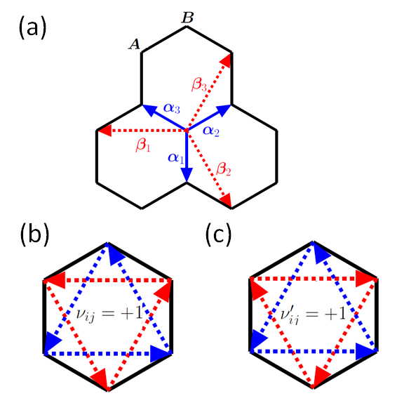
Figure 1: (color online)(a) The honeycomb lattice structure. (b) The directions along which $\nu_{ij}=+1$ has been shown, otherwise $\nu_{ij}=-1$. (c) The directions along which $\nu_{ij}^{\prime}=+1$ has been shown, otherwise $\nu_{ij}^{\prime}=-1$.

The ground state of the hamiltonian (Eq.1) is ferromagnetic for $J>-{3\sqrt{3}\over 2}\sum_{s}\left|D+sD^{\prime}\right|,\quad s=\pm 1$. We apply the Schwinger Boson mean field theory (SBMFT) to study the topological character of the low energy magnetic excitations at a finite temperature. The Schwinger Boson representation consists of the mapping the spin operators into spinons as, $S_{i}^{+}=c_{i,\uparrow}^{\dagger}c_{i,\downarrow}$, $S_{i}^{-}=c_{i,\downarrow}^{\dagger}c_{i,\uparrow}$, $S_{i}^{z}=\frac{1}{2}\left(c_{i,\uparrow}^{\dagger}c_{i,\uparrow}-c_{i,\downarrow}^{\dagger}c_{i,\downarrow}\right),$ where $c_{i,s}$ and $c_{i,s}^{\dagger}$ are the annihilation and creation operators of spin-1/2 up or down spinons respectively. The constraint $\sum_{s}c_{i,s}^{\dagger}c_{i,s}=2S$, $\forall i$ on the bosonic operators ensures the fulfillment of the spin-S algebra.

After applying Schwinger Boson transformation along with the constraint, and using a mean field approximation to reduce the 4-body operators to bilinear forms, the spin model Eq.1 is mapped to the the mean field hamiltonian,

$$\pazocal{H}= -\eta J\sum_{\left\langle i,j\right\rangle,s}\left[\hat{c}^{\dagger}_{i,s}\hat{c}_{j,s}+\mathtt{H.c.}\right]+\sum_{i,s}\left(\lambda-\frac{sB}{2}\right)\hat{c}^{\dagger}_{i,s}\hat{c}_{i,s}$$

$$+\frac{D}{2}\sum_{\left\langle\left\langle ij\right\rangle\right\rangle,s}\left[\left(i\nu_{ij}s\zeta_{-s}+s\xi_{-s}\right)\hat{c}^{\dagger}_{i,s}\hat{c}_{j,s}+\mathtt{H.c.}\right]$$

$$+\frac{D^{\prime}}{2}\sum_{\left\langle\left\langle ij\right\rangle\right\rangle,s}\left[\left(i\nu^{\prime}_{ij}s\zeta_{-s}+s\xi^{\prime}_{-s}\right)\hat{c}^{\dagger}_{i,s}\hat{c}_{j,s}+\mathtt{H.c.}\right]$$ (2)

where the mean field parameters are defined as, $\eta=\sum_{s}\left\langle\hat{\chi}_{ij,s}\right\rangle\equiv\sum_{s}\left\langle\hat{c}^{\dagger}_{i,s}\hat{c}_{j,s}\right\rangle$ evaluated on the nearest neighbour-bonds, and $\zeta=\zeta^{\prime}=\frac{1}{2}\left\langle\hat{\chi}_{ij,s}+\hat{\chi}_{ji,s}\right\rangle$, $\xi=\frac{\nu_{ij}}{2i}\left\langle\hat{\chi}_{ij,s}-\hat{\chi}_{ji,s}\right\rangle$ and $\xi^{\prime}=\frac{\nu^{\prime}_{ij}}{2i}\left\langle\hat{\chi}_{ij,s}-\hat{\chi}_{ji,s}\right\rangle$, evaluated on next nearest neighbour bonds. The terms associated with the parmeters $\eta,\nu_{ij}\zeta_{-s}$ of spinon Hamiltonian Eq2 constitute the Kane-Mele-Haldane modelKim et al. (2016). The term with parameter $\nu^{\prime}_{ij}\zeta_{-s}$ corresponds to the anti-chiral hopping term introduced in Ref.Colomés and Franz, 2018. The terms with the parameters $\xi_{s}$ and $\xi^{\prime}_{s}$ have no effect on the energy or the topological character of the bands, as the parameters are found to be much smaller compared to other mean field parameters. $\lambda$ is the Lagrange undetermined multiplier introduced to implement the local constraint. The mean field parameters are obtained by solving a set of self-consistent equations, derived by minimizing the Helmholtz free energy at a particular temperatureSM .

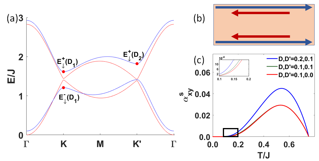
Figure 2: (color online)(a)band along symmetry lines $\Gamma K$, $KM$,$MK^{\prime}$,$K^{\prime}\Gamma$ for $J=1.0,B=0.1,D_{ch}=0.1,D_{Ach}=0.05,T=0.25$. The blue band is for down-spinon band and the red band is for up-spinon band. (b) The schematic of the antichiral contribution of the current from edge-states(blue-arrows) and bulk-states(red-arrows). (c) Nernst-conductivity v.s. temperature plot for different DMIs. The inset shows magnified figure of the rectangular portion of the figure.

Results.-

Band structure for spinons at a temperature T=0.25J is shown in Fig.2(a). In the absence of DMI, the two bands cross linearly at the Dirac points K and K^′Pershoguba et al. (2018). A finite DMI opens up a gap with magnitude $\Delta_{s}=3\sqrt{3}\left|D\zeta_{-s}\right|$ in each spinon sector at K and K^′Owerre (2016a, b, 2017); Pantaleón et al. (2019); Kim et al. (2016). For anisotropic system ($D_{A}\neq D_{B}$) considered here, the gap opening is not symmetric and leads to a tilting of the spinon bands near the Dirac momenta. The band tilting for each band in each spinon sector, defined as the energy difference between two Dirac-points in the same band, is given by, $T_{s}^{\tau}=3\sqrt{3}\left|D^{\prime}\zeta_{-s}\right|$. While the anti-chiral DMI drives the tilting of the bands, it has no effect on the magnitude of the band gap. Crucially, the tilting is opposite for the two species of spinons. For the parameters chosen in Fig.2(a), the gap and tilting for the up-spinon bands are smaller than those for the down spinon bands. This is because in the presence of positive magnetic field $B=0.1$ considered here, there are fewer down spinons and consequently, $\zeta_{\downarrow}<\zeta_{\uparrow}$.

The bands in each spinon sector carry non-zero Berry curvature. Spin Nernst effect has been proposed as a physical phenomenon to identify Berry curvature of spinon bands when there are comparable numbers of up and down spinons. Here we explore whether it can detect the existence of anti-chiral DMI. The Nernst conductivity has been calculated using the expression $\mathbin{\alpha^{s}_{xy}}{=\frac{1}{2V}\sum_{\mathbb{k},s,\tau}sc_{1}[\rho^{\tau}_{s}(\mathbb{k})]\Omega^{\tau}_{s}(\mathbb{k})}$Kim et al. (2016)^,Kovalev and Zyuzin (2016), where $\mathbin{\rho^{\tau}_{s}(\mathbb{k})}{=1/(\exp(E^{\tau}_{s}(\mathbb{k})/T)-1)}$ is the Bose-Einstein distribution and $\mathbin{\Omega^{\tau}_{s}(\mathbb{k})}{=i\sum_{\tau^{\prime}\neq\tau}\frac{\left\langle u^{\tau}_{s}(\mathbb{k})\middle|\frac{\partial\pazocal{H}}{\partial k_{x}}\middle|u^{\tau^{\prime}}_{s}(\mathbb{k})\right\rangle\left\langle u^{\tau^{\prime}}_{s}(\mathbb{k})\middle|\frac{\partial\pazocal{H}}{\partial k_{y}}\middle|u^{\tau}_{s}(\mathbb{k})\right\rangle-(k_{x}\leftrightarrow k_{y})}{(E^{\tau}_{s}(\mathbb{k})-E^{\tau^{\prime}}_{s}(\mathbb{k}))^{2}}}$. The results are plotted in Fig.2(c) for different $D$ and $D^{\prime}$. Increase in $D$ increases the band gap as well as the Berry curvature away from the Dirac-points. As a result, the Nernst conductivity is substantially affected by $D$ (Fig.2(c)). Conversely, since the Berry curvature is independent of $D^{\prime}$, the anti-chiral DMI has very little effect in the Nernst conductivity. The effect of $D^{\prime}$ on Nernst conductivity can be observed at low temperature due to tilting of the band structure(inset of Fig.2(c)). But at higher temperature, the $D^{\prime}$ has no influence in Nernst conductivity, because the contributions from higher bands overshadows the effects of band tilting. So, the presence of $D^{\prime}$ in the system is very hard to detect using Nernst conductivity. Instead, we suggest an alternative way to detect the presence of antichiral DMI.

The gapped bands are topologically non-trivial with Chern numbers $C_{\uparrow}^{-}=+1,C_{\uparrow}^{+}=-1,C_{\downarrow}^{-}=-1,C_{\downarrow}^{+}=+1$Matsuoka et al. (2005). Due to bulk-edge correspondence, we expect to observe edge states in a finite system. In the isotropic limit ($D_{A}=D_{B}$), the edge states are topologically protected by a chiral symmetry. The spinon currents along the two edges are equal and opposite for the up and down spinons. This results in a net flow of spins along the two edges in opposite directions – any scattering to the bulk states is prevented by symmetry constraints. For the asymmetric system considered here, $D^{\prime}$ induces an anti-chiral edge current of spinons where each species of spinon flows in the same direction along the two edges. This is balanced by couterflow current of spinons in the opposite direction carried by the bulk modes. The anti-chiral DMI breaks the chiral symmetry protecting the edge states and enables scattering between edge and bulk states. This edge-to-bulk scattering produces the bulk current that balances the anti-chiral edge current. In the following we discuss how the bulk and edge state dispersion changes due to interplay between the chiral and anti-chiral DMI.

Fig. 3 shows the spinon bands for a honeycomb nano-ribbon with dimension $200\times 500$ lattice sites with zigzag edges, together with the spin current profile along the width of the ribbon. Three different sets of $(D,D^{\prime})$ are chosen to illustrate the evolution of band dispersion and spin currents with changing DMI. For clarity of presentation, only one species of spinons is illustrated. Along with the total spin current, the contributions from the bulk and two edge modes are calculated separately to identify the effects of $D^{\prime}$ on each component. The spinon bands and the individual spin currents are color coded for easy identification. Green represents the bulk bands and their contribution to the spin current at each position along the width of the ribbon; red (blue) denotes the localized spinon mode and the associated spin current at the top (bottom) edge. A negative (positive) value of the spin current denotes spinon transport to the left (right) along the length of the ribbon.

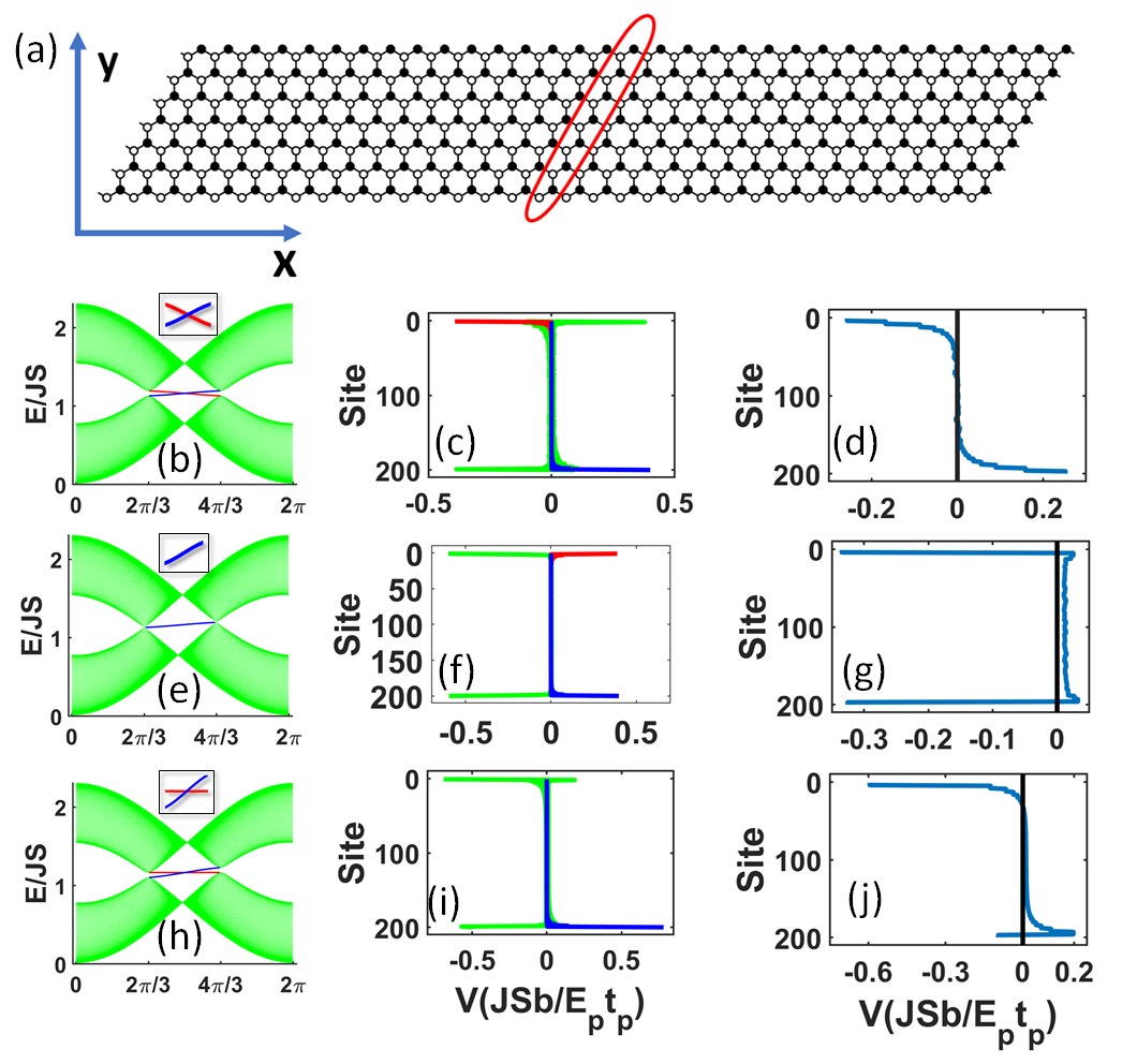
Figure 3: (color online)(a) A honeycomb ribbon. The encircled sites are the basis of unit cell. The figure sets $\left\{(b)-(d)\right\}$,$\left\{(e)-(g)\right\}$,$\left\{(h)-(j)\right\}$ represents result for down-spinon from $200\times 500$ stripe with DMIs $\left\{D=0.1,D^{\prime}=0.001\right\}$,$\left\{D=0.001,D^{\prime}=0.1\right\}$, $\left\{D=0.1,D^{\prime}=0.1\right\}$ respectively. The other parameters are $J=1.0,B=0.1,T=0.5$ for all the plots. The figure sets $\left\{(b),(e),(h)\right\}$ shows the band structure and inset of the figures shows the magnified dispersion of the edge states. The figure sets $\left\{(c),(f),(i)\right\}$ gives the spatial current distribution along width of the stripe. The figure sets $\left\{(d),(g),(j)\right\}$ shows the average of spatial current distribution over four sites respectively. In the figure sets $\left\{(b),(c),(e),(f),(h),(i)\right\}$ the green, red and blue plots corresponds to bulk-state, upper edge edge-state and lower-edge edge-state respectively. Moreover, the results for up-spinon is qualitatively same, the only difference is the dispersions are opposite for the bulk and edge states.

For $D>D^{\prime}$, the tilting of the bands is small and the dispersion of edge states at upper and lower edges are opposite, as shown in the Fig.3(c). The edge states are predominantly chiral in nature, and the spin current at the two edges are opposite in direction (though not equal in magnitude due to $D^{\prime}\neq 0$, which breaks chiral symmetry). For large $D^{\prime}$ ($D^{\prime}~{}\gg~{}D$), the tilting of the bands at the Dirac points is much greater and yields identical dispersion for the two edge states (Fig. 3(e)). This results in anti-chiral edge states where the spin current is in the same direction along both edges of the ribbon (Fig. 3(f)). Finally, when $D~{}\approx~{}D^{\prime}$, one of the edge states (the top edge in the present case) acquires a dispersionless character (Fig. 3(h)). In other words, the edge state at the top is localized with no spinon transport while the bottom edge has a finite dispersion with a finite edge current (Fig. 3(i)). Because of $U(1)$-symmetry of each spinon sector, there is a counter-propagating bulk current to compensate the imbalance between edge states. However, the bulk current is not uniform across the width of the ribbon. Instead, it is primarily confined to a small region near the edges. At each edge, the bulk current opposes the edge current, with its magnitude decreasing rapidly away from the edges.

We suggest that magnetic force microscopy(MFM) offers a promising experimental technique to measure the spinon current across the nano-ribbon and hence can detect the presence of anti-chiral edge states. Current MFM techniques can probe the local spin current in a finite sample to a resolution of a few nm. Since the topological character of the spinon bands for the different ranges of anisotropic DMI is reflected in distinct current profile across the ribbon, we believe MFM provides a promising experimental technique to identify anti-chiral edge states in real quasi-2D materials. Additionally, inelastic neutron scattering spectra can also indirectly detect the presence of anti-chiral edge modes, by probing the magnon band structure. If the bands are tilted or the energy at $K$ and $K^{\prime}$-point are unequal, it will suggest the presence of anti-chiral edge modes.

Finally, we show that the dynamical-spin structure factor(DSSF) at the edge of the materialSM defined as $\chi(\Omega)=i\sum_{l\in\text{edge}}\left[\chi_{ll}^{xx}(\Omega)+\chi_{ll}^{zz}(\Omega)\right],$ where, $\mathbin{\chi_{ij}^{\alpha\alpha}(\Omega)}{=-i\int^{\infty}_{-\infty}dte^{-i\Omega t}\left\langle\hat{S}^{\alpha}_{i}(t)\hat{S}^{\alpha}_{j}(0)\right\rangle_{0}}$ , offers a promising route to detecting anti-chiral edge states. The DSSF, shown in the figure Fig.4(a)-(b) for different edges, can be interpreted as the number of edge magnons present in a given energy level, and is proportional to the product of the density of states and Bose-Einstein distribution for the corresponding energy level. The signature of the edge states is reflected in the features of the DSSF near $\Omega=\frac{3J}{2}+B$, which is the energy of the edge states in the absence of any DMI. Our results show that $\chi(\Omega)$ is dramatically different for the two edges, when $\left|D\right|\approx\left|D^{\prime}\right|$(equivalently $D_{A}\gg D_{B}$ or $D_{B}\gg D_{A}$). The DSSF can be measured using the experimental set-up shown in Fig.4(c), according to referenceJoshi et al. (2018). The quantum fluctuation of the spins at the edges gives rise to spin current in metal and as a consequence the spin current gives rise to the charge current in transverse direction due to inverse spin Hall effect. Measurement of the noise-spectrum in the charge current gives the information of the DSSF.

The presence of anti-chiral DMI requires two in-equivalent sub-lattices in the 2D-honeycomb lattice, as shown in Fig.4(d). The presence of two different types of atoms will result in asymmetric DMI, leading to a broken inversion symmetry and non-zero $D^{\prime}$. Mirror symmetry along the dotted lines prevents any non-zero perpendicular DMI on nearest-neighbour bonds, whereas in-plane mirror symmetry suppresses any in-plane DMI. While we

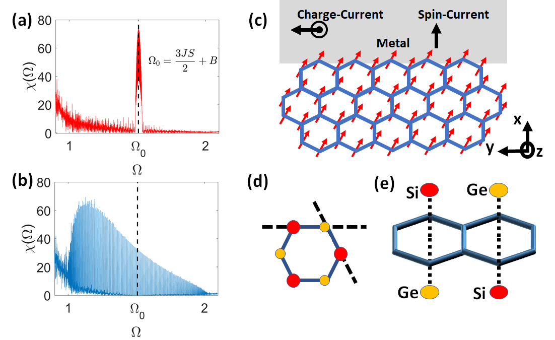
Figure 4: (color online) (color online) (a)-(b) Dynamical spin structure factor for two edges at temperature $T=0.4J$, with parameters $D=0.1,D^{\prime}=0.09,B=0.01$. Red and blue colors denote upper and lower edges. (c) The experimental setup for spin Hall noise spectroscopy. (d) A ferromagnetic material with two different sub-latices with a mirror symmetric plane along the dashed lines. (e) A proposed material based on real materials CrGeTe3 and CrSiTe3 to realize antichiral edge states.

are not aware of any such material at present, the recent discovery of ferromagnetic order in 2D limit of several Cr-based compounds including CrI3 Chen et al. (2018), CrBr3 Samuelsen et al. (1971); Tsubokawa (1960); Williams et al. (2015a), CrSrTe3Williams et al. (2015b) and CrGeTe3Gong et al. (2017) as well as the Fe-based family of compounds AFe_2(PO_4)_2 (A=Ba,Cs,K,La)Kim and Kee (2017) offer great promise. These quasi-2D materials consist of weakly Van Der Waals-coupled honeycomb ferromagets. Presence of chiral DMI in some members of this family Chen et al. (2018)has been established using inelastic neutron scattering spectroscopy. In materials like CrSrTe3 and CrGeTe3, presence of inversion center at the center of honeycomb cell makes the two sub-lattices equivalent. The inversion symmetry can be removed by replacing every other Ge atom by an Si atom as depicted in Fig.4(e). In a similar vein, replacement of P atom by another Group V element in AFe_2(PO_4)_2 (A=Ba,Cs,K,La)Kim and Kee (2017) will break the inversion symmetry of the lattice. The breaking of inversion symmetry may, in principle, give rise to additional interactions in these materials, e.g., nearest neighbor DMI. However, we have verified that inclusion of additional interactions, including nearest neighbor DMI as well as 2nd and 3rd nearest neighbor Heisenberg interactions only modifies the linear dispersion of the edge states, and does not suppress the appearance of anti-chiral edge statesSM .

In conclusion, we have studied a Heisenberg ferromagnet with additional next nearest neighbor DMIs on a honeycomb lattice with broken sublattice symmetry. The unequal DMI between atoms on different sublattices, together with the broken chiral symmetry results in the emergence of anti-chiral edge states, in addition to the normal chiral modes. This is manifested in unique spin current distribution across the width of a finite system with ribbon geometry. We propose experimental probes to detect the presence of anti-chiral edge states as well as a potential material where such states may be realized experimentally.

Financial support from the Ministry of Education, Singapore, in the form of grant MOE2016-T2-1-065 is gratefully acknowledged.

I Schwinger Boson Mean Field Theory

The parent spin Hamiltonian is,

$$\pazocal{H}= -J\sum_{\left\langle i,j\right\rangle}\bm{S}_{i}\cdot\bm{S}_{j}+D\sum_{\left\langle\left\langle i,j\right\rangle\right\rangle}\nu_{ij}\hat{z}\cdot\left(\bm{S}_{i}\times\bm{S}_{j}\right)$$

$$+D^{\prime}\sum_{\left\langle\left\langle i,j\right\rangle\right\rangle}\nu_{ij}^{\prime}\hat{z}\cdot\left(\bm{S}_{i}\times\bm{S}_{j}\right)-B\sum_{i}S_{i}^{z},$$ (3)

After implementing the Schwinger boson transformation and imposing the constraints, the spinon Hamiltonian reads,

$$\pazocal{H}_{sp}= -\frac{J}{2}\sum_{\left\langle i,j\right\rangle}\left(\hat{c}^{\dagger}_{i,\uparrow}\hat{c}^{\dagger}_{j,\downarrow}\hat{c}_{i,\downarrow}\hat{c}_{j,\uparrow}+\hat{c}^{\dagger}_{i,\downarrow}\hat{c}^{\dagger}_{j,\uparrow}\hat{c}_{i,\uparrow}\hat{c}_{j,\downarrow}\right)$$

$$-\frac{J}{4}\left(\hat{c}^{\dagger}_{i,\uparrow}\hat{c}_{i,\uparrow}\hat{c}^{\dagger}_{j,\uparrow}\hat{c}_{j,\uparrow}+\hat{c}^{\dagger}_{i,\downarrow}\hat{c}_{i,\downarrow}\hat{c}^{\dagger}_{j,\downarrow}\hat{c}_{j,\downarrow}+\hat{c}^{\dagger}_{i,\uparrow}\hat{c}_{i,\uparrow}\hat{c}^{\dagger}_{j,\uparrow}\hat{c}_{j,\uparrow}+\hat{c}^{\dagger}_{i,\downarrow}\hat{c}_{i,\downarrow}\hat{c}^{\dagger}_{j,\downarrow}\hat{c}_{j,\downarrow}\right)$$

$$+\frac{iD}{2}\sum_{\left\langle\left\langle i,j\right\rangle\right\rangle}\nu_{ij}\left(\hat{c}^{\dagger}_{i,\uparrow}\hat{c}_{i,\downarrow}\hat{c}^{\dagger}_{j,\downarrow}\hat{c}_{j,\uparrow}-\hat{c}^{\dagger}_{i,\downarrow}\hat{c}_{i,\uparrow}\hat{c}^{\dagger}_{j,\uparrow}\hat{c}_{j,\downarrow}\right)$$

$$+\frac{iD^{\prime}}{2}\sum_{\left\langle\left\langle i,j\right\rangle\right\rangle}\nu^{\prime}_{ij}\left(\hat{c}^{\dagger}_{i,\uparrow}\hat{c}_{i,\downarrow}\hat{c}^{\dagger}_{j,\downarrow}\hat{c}_{j,\uparrow}-\hat{c}^{\dagger}_{i,\downarrow}\hat{c}_{i,\uparrow}\hat{c}^{\dagger}_{j,\uparrow}\hat{c}_{j,\downarrow}\right)$$

$$-\frac{B}{2}\sum_{i}\left(\hat{c}^{\dagger}_{i,\uparrow}\hat{c}_{i,\uparrow}-\hat{c}^{\dagger}_{i,\downarrow}\hat{c}_{i,\downarrow}\right)+\sum_{i}\lambda_{i}\left(\hat{c}^{\dagger}_{i,\uparrow}\hat{c}_{i,\uparrow}+\hat{c}^{\dagger}_{i,\downarrow}\hat{c}_{i,\downarrow}-2S\right)$$

$$+3NJS^{2}-4SN\lambda$$ (4)

The bond operators have to be choosen such that the total number of spinon is conserved in the mean field Hamiltoian which is equivalent to $S_{z}$-conservation in terms of spinLee et al. (2015). Defining the bond-operators, $\hat{\chi}_{ij}=\hat{c}^{\dagger}_{i,s}\hat{c}_{j,s}$ and $\hat{\chi}_{ij}=\left(\hat{\chi}_{ij,\uparrow}+\hat{\chi}_{ij,\downarrow}\right)/2$, we can re-write the Hamiltonian as,

$$\pazocal{H}_{sp}= -2J\sum_{\left\langle i,j\right\rangle}:\hat{\chi}_{ij}^{\dagger}\hat{\chi}_{ij}:$$

$$-\frac{D}{2}\sum_{\left\langle\left\langle i,j\right\rangle\right\rangle}i\nu_{ij}\left(:\hat{\chi}_{ij,\uparrow}^{\dagger}\hat{\chi}_{ij,\downarrow}:-:\hat{\chi}_{ij,\downarrow}^{\dagger}\hat{\chi}_{ij,\uparrow}:\right)$$

$$-\frac{D^{\prime}}{2}\sum_{\left\langle\left\langle i,j\right\rangle\right\rangle}i\nu^{\prime}_{ij}\left(:\hat{\chi}_{ij,\uparrow}^{\dagger}\hat{\chi}_{ij,\downarrow}:-:\hat{\chi}_{ij,\downarrow}^{\dagger}\hat{\chi}_{ij,\uparrow}:\right)$$

$$-\frac{B}{2}\sum_{i}\left(\hat{c}^{\dagger}_{i,\uparrow}\hat{c}_{i,\uparrow}-\hat{c}^{\dagger}_{i,\downarrow}\hat{c}_{i,\downarrow}\right)$$

$$+\lambda\sum_{is}\hat{c}^{\dagger}_{i,s}\hat{c}_{i,s}-4SN\lambda+3NJS^{2}$$ (5)

New bond operators are defined so that corresponding mean field parameters are real: $\hat{A}_{ij,s}=\frac{1}{2}\left(\hat{\chi}_{ij,s}+\hat{\chi}_{ji,s}\right)$, $\hat{B}_{ij,s}=\frac{\nu_{ij}}{2i}\left(\hat{\chi}_{ij,s}-\hat{\chi}_{ji,s}\right)$, $\hat{B^{\prime}}_{ij,s}=\frac{\nu^{\prime}_{ij}}{2i}\left(\hat{\chi}_{ij,s}-\hat{\chi}_{ji,s}\right)$. Defining mean field parameters $\eta=\left\langle\hat{\chi}_{ij}^{\dagger}\right\rangle=\left\langle\hat{\chi}_{ij}\right\rangle$, $\zeta_{s}=\left\langle\hat{A}_{ij,s}^{\dagger}\right\rangle=\left\langle\hat{A}_{ij,s}\right\rangle$, $\xi_{s}=\left\langle\hat{B}_{ij,s}^{\dagger}\right\rangle=\left\langle\hat{B}_{ij,s}\right\rangle$, $\xi^{\prime}_{s}=\left\langle\hat{B^{\prime}}_{ij,s}^{\dagger}\right\rangle=\left\langle\hat{B^{\prime}}_{ij,s}\right\rangle$, the quartic terms of Hamiltonian can be decoupled into quadratic and the mean-field spinon Hamiltonian takes the form as,

$$\pazocal{H}_{sp}^{mf}= -\eta J\sum_{\left\langle i,j\right\rangle,s}\left[\hat{c}^{\dagger}_{i,s}\hat{c}_{j,s}+\mathtt{H.c.}\right]$$

$$+\frac{D}{2}\sum_{\left\langle\left\langle ij\right\rangle\right\rangle,s}\left[i\nu_{ij}s\zeta^{ch}_{-s}\hat{c}^{\dagger}_{i,s}\hat{c}_{j,s}+\mathtt{H.c.}\right]$$

$$+\frac{D}{2}\sum_{\left\langle\left\langle ij\right\rangle\right\rangle,s}\left[s\xi^{ch}_{-s}\hat{c}^{\dagger}_{i,s}\hat{c}_{j,s}+\mathtt{H.c.}\right]$$

$$+\frac{D^{\prime}}{2}\sum_{\left\langle\left\langle ij\right\rangle\right\rangle,s}\left[i\nu^{\prime}_{ij}s\zeta^{Ach}_{-s}\hat{c}^{\dagger}_{i,s}\hat{c}_{j,s}+\mathtt{H.c.}\right]$$

$$+\frac{D^{\prime}}{2}\sum_{\left\langle\left\langle ij\right\rangle\right\rangle,s}\left[s\xi^{Ach}_{-s}\hat{c}^{\dagger}_{i,s}\hat{c}_{j,s}+\mathtt{H.c.}\right]$$

$$+\sum_{i,s}\left(\lambda-\frac{sB}{2}\right)\hat{c}^{\dagger}_{i,s}\hat{c}_{i,s}$$

$$+6NJ\eta^{2}-6DN\sum_{s}s\zeta_{s}\xi_{-s}-6D^{\prime}N\sum_{s}s\zeta_{s}\xi^{\prime}_{-s}-4SN\lambda+3NJS^{2}$$ (6)

Fourier transformation of the mean field Hamiltonian to momentum-space yields,

$$\pazocal{H}_{sp}^{mf}=\sum_{\bm{k}\in\mathtt{B.Z.},s}\Psi^{\dagger}_{\bm{k},s}\left[g_{s}(\bm{k})I+\bm{h}_{s}(\bm{k})\cdot\bm{\sigma}\right]\Psi_{\bm{k},s}+E_{0},$$ (7)

where, $\Psi_{\bm{k},s}^{\dagger}=\left(\hat{a}_{\bm{k},s}^{\dagger},\hat{b}_{\bm{k},s}^{\dagger}\right)$. $\hat{a}_{\bm{k},s}^{\dagger}$ and $\hat{b}_{\bm{k},s}^{\dagger}$ are the creation operators for Schwinger bosons on sublattice-A and sublattice-B (see Fig.1(a) of main text), respectively. $\bm{\sigma}_{\alpha}$($\alpha=x,y,z$) represents the Pauli matrices. The other terms are given by,

$$g_{s}(\bm{k})= -\frac{sB}{2}+\lambda+sD\xi_{-s}\gamma_{c}^{\beta}+sD^{\prime}\left(\xi^{\prime}_{-s}\gamma_{c}^{\beta}-\zeta_{-s}\gamma_{s}^{\beta}\right),$$

$$h_{s}(\bm{k})= \begin{pmatrix}-J\eta\gamma_{c}^{\alpha}\\ J\eta\gamma_{s}^{\alpha}\\ -Ds\zeta_{-s}^{c}\gamma_{s}^{\beta}\end{pmatrix},$$

$$E_{0}= 6NJ\eta^{2}-6DN\sum_{s}s\zeta_{s}\xi_{-s}-6D^{\prime}N\sum_{s}s\zeta_{s}\xi^{\prime}_{-s}-4SN\lambda+3NJS^{2},$$ (8)

where, $\gamma_{c}^{\beta}=\sum_{j}\cos(\bm{k}\cdot\bm{\beta}_{j}),\gamma_{s}^{\beta}=\sum_{j}\sin(\bm{k}\cdot\bm{\beta}_{j}),\gamma_{c}^{\alpha}=\sum_{j}\cos(\bm{k}\cdot\bm{\alpha}_{j}),\gamma_{s}^{\alpha}=\sum_{j}\sin(\bm{k}\cdot\bm{\alpha}_{j})$ and the vectors $\bm{\beta}_{j}$ and $\bm{\alpha}_{j}$ are shown in figure Fig.1(a). $N$ is the number of unit cells in lattice. $E_{0}$ is the energy of the ground state and the energies of spinons are considered with respect to the ground state energy.

After diagonalizing the k-space Hamiltonian we get,

$$\pazocal{H}_{sp}^{mf}=E_{0}+\sum_{\bm{k},s,\tau}E_{s}^{\tau}(\bm{k})\hat{c}^{\dagger}_{\bm{k},\tau,s}\hat{c}_{\bm{k},\tau,s},$$ (9)

where, the relative energies,

$$E_{s}^{\tau}(\bm{k})=g_{s}(\bm{k})+\tau\left|h_{s}(\bm{k})\right|,$$ (10)

refer to the upper ($\tau=+1$) and the lower ($\tau=-1$) band for each spinon sectors $s=\pm 1$.

From this we get the internal energy and the entropy of the non-interacting system as,

$$U =E_{0}+\sum_{\bm{k},s,\tau}\rho_{s}^{\tau}(\bm{k})E_{s}^{\tau}(\bm{k}),$$

$$S =k_{B}\sum_{\bm{k},s,\tau}[\left(1+\rho_{s}^{\tau}(\bm{k})\right)\ln\left(1+\rho_{s}^{\tau}(\bm{k})\right)-\rho_{s}^{\tau}(\bm{k})\ln\rho_{s}^{\tau}(\bm{k})],$$ (11)

where, $\rho_{s}^{\tau}(\bm{k})=\left[\exp\left(E^{\tau}_{s}(\bm{k})\right)-1\right]^{-1}$ is the Bose-Einstein distribution of spin-s spinons in the $\tau$-band. The Helmohltz-free-energy is given by,

$$G =U-TS$$

$$=E_{0}-{k_{B}T}\sum_{\bm{k},s,\tau}\ln\left(\frac{1}{1-\exp\left(\frac{-E_{s}^{\tau}(\bm{k})}{k_{B}T}\right)}\right)$$ (12)

After minimizing the Helmholtz free energy with respect to the mean field parameters, we get six self consistent equations, given by,

$$2S= \frac{1}{2N}\sum_{\bm{k},\tau,s}\rho_{s}^{\tau}(\bm{k})$$

$$1=- \frac{J}{12N}\sum_{\bm{k},s,\tau}\tau\frac{\rho_{s}^{\tau}(\bm{k})}{\left|h_{s}\right|}\left|\sum_{j}e^{i\bm{k}\cdot\bm{\alpha}_{j}}\right|^{2}$$

$$D\xi_{s}+D^{\prime}\xi^{\prime}_{s}= \frac{1}{6N}\sum_{\bm{k},\tau}\left(D^{\prime}-\tau s\frac{D^{2}\zeta_{-s}\gamma}{h_{s}}\right)\rho_{s}^{\tau}(\bm{k})\gamma_{s}^{\beta}$$

$$\zeta_{s}= \frac{1}{6N}\sum_{\bm{k},\tau}\rho^{\tau}_{s}(\bm{k})\sum_{j}\cos(\bm{k}\cdot\bm{\beta}_{j}),$$ (13)

The mean field parameters are obtained by solving these six self-consistent equations. It is notable that the mean field parameter $\eta$ can be chosen as real, absorbing the complex phase factor into operator $\hat{c}_{i,s}$. All other mean field parameters already chosen to be real. Using the parameters, we plot the band structure and evaluate corresponding topological information. For a fixed set of $J,D,D^{\prime},B$, the mean field parameters are solved and plotted against temperature $T$ in Fig5. The parameters $\eta$ and $\zeta_{s}$ represent short range correlations identifying magnetic ordering and serve as order parameters for the ferromagnetic to paramegnetic transition at higher temperaturesSarker et al. (1989). The constraint $\lambda$ is considered uniform throughout the lattice to retain the translational symmetry of the lattice.

At low temperatures, finite, non-zero values of $\eta$ and $\zeta_{\uparrow}$ denote ferromagnetic ordering. A positive $B$ determines that the spins are all aligned along the +ve x-direction at $T=0$. In other words, the system is populated with up-spinons. As the temperature increases, thermally excited down-spinons are generated, resulting in a finite, non-zero $\zeta_{\downarrow}$. Finally at high temperatures, a vanishing of all the mean field parameters denote a transition to the paramagnetic phase. The paramagnetic phase transition with all zero correlations to be expected to be an outcome of large-N expansion. It has been shown for Heisenberg model that taking into account of the quantum fluctuations in the mean field parameter removes the phase transitionTchernyshyov and Sondhi (2002).

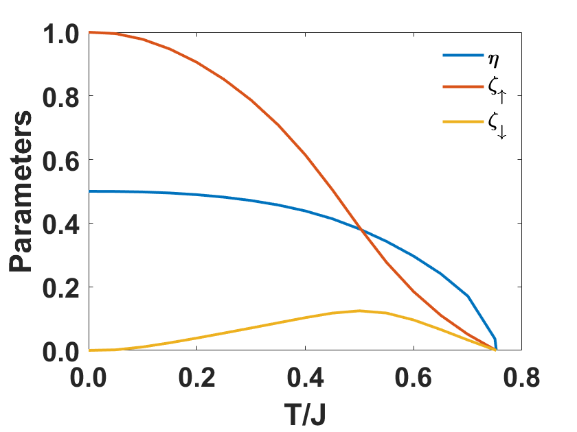
Figure 5: (color online)Plot of mean-field parameters, for $J=1.0,D=0.1,D^{\prime}=0.05,B=0.1$

II Calculation of the edge-state and velocity distribution on a stripe geometry

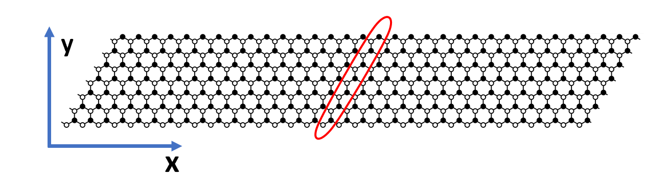
Figure 6: (color online)The honeycomb lattice structure of size ($20\times 14$) with periodic boundary condition along x-axis and open boundary condition along y-axis. The encircled sites are the basis of unit cell.

The Hamiltonian in tight binding Hamiltonian can be written as,

$$\pazocal{H}=\sum_{ij}t_{ij}\ket{i}\bra{j},$$ (14)

where, i and j are the sites of lattice and $t_{ij}$ is the hopping amplitude. More explicitly the Hamiltonian can be written as a matrix form asGuclu et al. (2014),

$$\pazocal{H}=\sum_{m,s}\left[\Psi_{m,s}^{\dagger}U_{s}\Psi_{m,s}+\Psi_{m,s}^{\dagger}T_{s}\Psi_{m+1,s}+\Psi_{m+1,s}^{\dagger}T_{s}^{\dagger}\Psi_{m,s}\right],$$ (15)

where, $\Psi_{m,s}^{\dagger}=(\hat{b}_{1,m,s}^{\dagger},\hat{a}_{2,m,s}^{\dagger},...,\hat{a}_{N,m,s}^{\dagger},)$ and $N$ is the number of sites along the stripe(the sites inside the red circle of Fig.6 makes one stripe) and $m$ denotes the stripe index and $s$-denotes up or down spinon type. $U$ and $T$ are $N\times N$ matrices. Matrix-$U$ contains all the onsite and intra-stripe hopping elements(inside the red circle of Fig.6) and matrix-$T$ contains all the inter-stripe hopping elements.

Imposing periodic boundary condition along the longitudinal direction as shown in the figure6, one can Fourier transform the Hamiltonian with a 1D Bloch-wave vector, given by $\Psi_{m}=(1/\sqrt{M})\sum_{k=0}^{M-1}\Psi_{k}e^{-i2\pi km/M}$, where $M$ is the number of stripes along x-axis in Fig.6. After Fourier transform the Hamiltonian can be written as,

$$H =\sum_{k}\Psi^{\dagger}_{k}\left[U+\left(Te^{i\frac{2k\pi}{M}}+\text{H.c.}\right)\right]\Psi_{k}$$

$$=\sum_{k}\Psi^{\dagger}_{k}H_{k}\Psi_{k},$$ (16)

The Hamiltonian can be diagonalized as,

$$\epsilon_{k}=P^{\dagger}H_{k}P,$$ (17)

where, $P$ is an unitary matrix and the corresponding eigenvector is given by,

$$\Psi_{k}^{d}=P^{\dagger}\Psi_{k}$$ (18)

Diagonalizing the momentum space Hamiltonian, we obtain the bands for the stripe geometry, as shown in the figures Fig.3(b), 3(e), 3(h) of the main text.

The velocity operator, used to evaluate the spinon transport properties, are expressed in terms of the k-space eigenstates asD. Mahan (2000)Laurent ,

$$\hat{v}=\sum_{ij}v_{ij}\ket{i}\bra{j},$$ (19)

where the coefficients $v_{ij}$ is given by,

$$v_{ij}=\bra{i}\hat{v}\ket{j}=-\frac{i}{\hbar}\bra{i}[\hat{r},\pazocal{H}]\ket{j}=-\frac{i}{\hbar}(\bm{r}_{i}-\bm{r}_{j})t_{ij}.$$ (20)

We have calculated the distribution of the velocity component along x-axis across the cross section of the ribbon, which are shown in figure Fig.3(c),3(f),3(i) of the main text.

III Calculation of the dynamical spin structure factor

To calculate the dynamical spin structure factor, we have used the Holstein-Primakoff transformation, given by,

$$\hat{S}^{x}_{m}=\frac{1}{2}\left(\hat{a}_{m}+\hat{a}_{m}^{\dagger}\right),$$

$$\hat{S}^{y}_{m}=\frac{i}{2}\left(\hat{a}_{m}-\hat{a}_{m}^{\dagger}\right),$$

$$\hat{S}^{z}_{m}=S-\hat{a}_{m}^{\dagger}\hat{a}_{m},$$ (21)

where, $\hat{a}_{m}^{\dagger}$ and $\hat{a}_{m}$ are the creation annihilation operators of Holstein-Primakoff bosons. For the case of ferromagnet with up spin at each site, the Holstein-Primakoff boson represents the down-spinons in Schwinger boson picture at low temperature. The diagonalized Hamiltonian can be written as,

$$H_{k}=\sum_{n}\epsilon_{n}(k)\hat{a}_{n,k}^{d\dagger}\hat{a}_{n,k}^{d},$$ (22)

where, $\hat{a}^{d}_{n,k}$ is the bosonic operator after diagonalization. Using the above relation and Heisenberg’s equation of motion it can be proved that,

$$\hat{a}_{n,k}^{d\dagger}(t) =\hat{a}_{n,k}^{d\dagger}(0)e^{i\epsilon_{n}(k)t}$$

$$\hat{a}_{n,k}^{d}(t) =\hat{a}_{n,k}^{d}(0)e^{-i\epsilon_{n}(k)t}$$ (23)

The dynamical spin structure factor in terms of Holstein-Primakoff Boson, is given by,

$$\chi(\Omega) =\sum_{m\in\text{edge}}\left[\chi^{xx}_{mm}(\Omega)+\chi^{zz}_{mm}(\Omega)\right]$$

$$=\sum_{m\in\text{edge}}\left[\int^{\infty}_{-\infty}dte^{-i\Omega t}\left(-i\left\langle\hat{S}^{x}_{1,m}(t)\hat{S}^{x}_{1,m}(0)\right\rangle\right)+\int^{\infty}_{-\infty}dte^{-i\Omega t}\left(-i\left\langle\hat{S}^{z}_{1,m}(t)\hat{S}^{z}_{1,m}(0)\right\rangle\right)\right]$$

$$=-i\sum_{m}\int^{\infty}_{-\infty}dte^{-i\Omega t}\left[\frac{S}{2}\left\langle\hat{a}_{1,m}(t)\hat{a}_{1,m}(0)+\hat{a}_{1,m}(t)\hat{a}_{1,m}^{\dagger}(0)+\hat{a}_{1,m}^{\dagger}(t)\hat{a}_{1,m}(0)+\hat{a}_{1,m}^{\dagger}(t)\hat{a}_{1,m}(0)\right\rangle\right.$$

$$\qquad\qquad\qquad\left.+\left\langle S^{2}-S\hat{a}_{1,m}^{\dagger}(0)\hat{a}_{1,m}(0)-S\hat{a}^{\dagger}_{1,m}(t)\hat{a}_{1,m}(t)\right\rangle\right]\qquad\qquad\text{[Neglecting the higer order terms]}.$$ (24)

Transforming the boson operator $\hat{a}_{1,m}(t)$ into diagonalized boson operator $\hat{a}^{d}_{1,m}(t)$ and using the relation Eq.23, we derive the spin-structure factor.

IV Modulation of edge state dispersion in presence of other interactions in a honeycomb ferromagnet

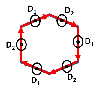
Figure 7: (color online) DM-interactions on nearest neighbour bonds.

The spin Hamiltonian studied in theis work is an idealized model. For example, the long range Heisenberg interactions are neglected. Moreover, the breaking of inversion symmetry required for anti-chiral DM-term $D^{\prime}$ might give rise the nearest neighbour out of plane DM-interactions and also in plane DM-interactions. At low temperature, the in plane interactions can be neglected, which gives rise to three magnon interactions in terms of Holstein Primakoff Bosons. Neglecting, any presence of in plane DM-interaction at low temperature, we can re-write a more general Hamiltonian of the material as,

$$\pazocal{H}=J_{1}\sum_{\left\langle i,j\right\rangle}\bm{S}_{i} \cdot\bm{S}_{j}+J_{2}\sum_{\left\langle\left\langle i,j\right\rangle\right\rangle}\bm{S}_{i}\cdot\bm{S}_{j}+J_{3}\sum_{\left\langle\left\langle\left\langle i,j\right\rangle\right\rangle\right\rangle}\bm{S}_{i}\cdot\bm{S}_{j}$$

$$+D_{1}\sum_{\left\langle ij\right\rangle_{A}}\nu_{ij}\hat{z}\cdot(\bm{S}_{i}\times\bm{S}_{j})+D_{2}\sum_{\left\langle ij\right\rangle_{B}}\nu_{ij}\hat{z}\cdot(\bm{S}_{i}\times\bm{S}_{j})$$

$$+D\sum_{\left\langle\left\langle ij\right\rangle\right\rangle_{B}}\nu_{ij}\hat{z}\cdot(\bm{S}_{i}\times\bm{S}_{j})+D^{\prime}\sum_{\left\langle\left\langle ij\right\rangle\right\rangle_{B}}\nu^{\prime}_{ij}\hat{z}\cdot(\bm{S}_{i}\times\bm{S}_{j})$$

$$+B\sum_{i}\bm{S}_{i},$$ (25)

where, the DM-interactions $D_{1}$ and $D_{2}$ are defined on the nearest neighbour bonds $\left\langle ij\right\rangle_{A}$ and $\left\langle ij\right\rangle_{B}$ as shown in Fig.7. Any single ion anisotropy terms acts as chemical potential for the spin-excitation, and is accounted for by a renormalization of the magnetic field. As a more realistic model, we have fixed the Heisenberg interactions present in the material CrI3Chen et al. (2018), $J_{1}=2.09$ meV, $J_{2}=0.16$ meV, $J_{3}=0.18$ meV. The nearest neighbour DM-terms and magentic field are fixed as $D_{1}=0.1$ meV, $D_{2}=0.15$ meV, $B=g\mu_{B}B_{z}=0.01$ meV. We transformed the spin Hamiltonian into magnon Hamiltonian using Holstein Primakoff transformation defined in Eq.21. Then, plotted the band structure and dynamical spin structure factor in Fig8. Our results confirm that the qualitative behaviour is same as the ideal model considered in the test and the behaviour of edge states mostly depends on the DM-interactions $D$ and $D^{\prime}$. The presence of other interaction terms in the Hamiltonian just distorts the linear dispersion of the edge states to a non-linear dispersion.

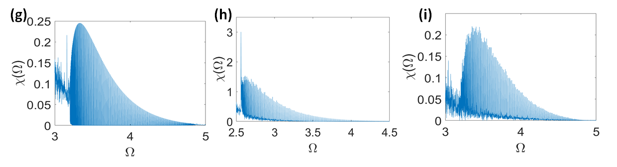
Figure 8: (color online) Band structure of magnons of a stripe geometry for parameters (a) $D=0.31meV$, $D^{\prime}=0.01meV$, (b) $D=0.31meV$, $D^{\prime}=0.28meV$, (c) $D=0.01meV$, $D^{\prime}=0.31meV$. The dynamical spin structure factor for upper edge at $T=0.4$ for parameters, (d) $D=0.31meV$, $D^{\prime}=0.01meV$, (e) $D=0.31meV$, $D^{\prime}=0.28meV$, (f) $D=0.01meV$, $D^{\prime}=0.38meV$. The dynamical spin structure factor for lower edge at $T=0.4$ for parameters, (g) $D=0.31meV$, $D^{\prime}=0.01meV$, (h) $D=0.31meV$, $D^{\prime}=0.28meV$, (i) $D=0.01meV$, $D^{\prime}=0.38meV$.

References

- Haldane (1988) F. D. M. Haldane, Phys. Rev. Lett. 61, 1029 (1988).
- Chen et al. (2018) L. Chen, J.-H. Chung, B. Gao, T. Chen, M. B. Stone, A. I. Kolesnikov, Q. Huang, and P. Dai, Phys. Rev. X 8, 041028 (2018).
- Kim and Kee (2017) H.-S. Kim and H.-Y. Kee, npj Quantum Materials 2, 20 (2017).
- Kim et al. (2016) S. K. Kim, H. Ochoa, R. Zarzuela, and Y. Tserkovnyak, Phys. Rev. Lett. 117, 227201 (2016).
- Zyuzin and Kovalev (2016) V. A. Zyuzin and A. A. Kovalev, Phys. Rev. Lett. 117, 217203 (2016).
- Cheng et al. (2016) R. Cheng, S. Okamoto, and D. Xiao, Phys. Rev. Lett. 117, 217202 (2016).
- Zhang et al. (2018) Y. Zhang, S. Okamoto, and D. Xiao, Phys. Rev. B 98, 035424 (2018).
- Onose et al. (2010) Y. Onose, T. Ideue, H. Katsura, Y. Shiomi, N. Nagaosa, and Y. Tokura, Science 329, 297 (2010).
- Hirschberger et al. (2015) M. Hirschberger, J. W. Krizan, R. J. Cava, and N. P. Ong, Science 348, 106 (2015).
- Ideue et al. (2012) T. Ideue, Y. Onose, H. Katsura, Y. Shiomi, S. Ishiwata, N. Nagaosa, and Y. Tokura, Phys. Rev. B 85, 134411 (2012).
- Hentrich et al. (2019) R. Hentrich, M. Roslova, A. Isaeva, T. Doert, W. Brenig, B. Büchner, and C. Hess, Phys. Rev. B 99, 085136 (2019).
- Colomés and Franz (2018) E. Colomés and M. Franz, Phys. Rev. Lett. 120, 086603 (2018).
- Mandal et al. (2019) S. Mandal, R. Ge, and T. C. H. Liew, Phys. Rev. B 99, 115423 (2019).
- Vila et al. (2019) M. Vila, N. T. Hung, S. Roche, and R. Saito, Phys. Rev. B 99, 161404(R) (2019).
- Pershoguba et al. (2018) S. S. Pershoguba, S. Banerjee, J. C. Lashley, J. Park, H. Ågren, G. Aeppli, and A. V. Balatsky, Phys. Rev. X 8, 011010 (2018).
- Owerre (2016a) S. A. Owerre, Journal of Physics Condensed Matter 28, 386001 (2016a).
- Owerre (2016b) S. A. Owerre, Journal of Applied Physics 120, 043903 (2016b).
- Owerre (2017) S. A. Owerre, Journal of Physics Communications 1, 021002 (2017).
- Pantaleón et al. (2019) P. A. Pantaleón, R. Carrillo-Bastos, and Y. Xian, Journal of Physics: Condensed Matter 31, 085802 (2019).
- (20) Supplementary Matrial .
- Kovalev and Zyuzin (2016) A. A. Kovalev and V. Zyuzin, Phys. Rev. B 93, 161106(R) (2016).
- Matsuoka et al. (2005) E. Matsuoka, K. Hayashi, A. Ikeda, K. Tanaka, T. Takabatake, and M. Matsumura, Journal of the Physical Society of Japan 74, 1382 (2005).
- Joshi et al. (2018) D. G. Joshi, A. P. Schnyder, and S. Takei, Phys. Rev. B 98, 064401 (2018), arXiv:1803.11239 [cond-mat.str-el] .
- Samuelsen et al. (1971) E. J. Samuelsen, R. Silberglitt, G. Shirane, and J. P. Remeika, Phys. Rev. B 3, 157 (1971).
- Tsubokawa (1960) I. Tsubokawa, Journal of the Physical Society of Japan 15, 1664 (1960).
- Williams et al. (2015a) T. J. Williams, A. A. Aczel, M. D. Lumsden, S. E. Nagler, M. B. Stone, J.-Q. Yan, and D. Mandrus, Phys. Rev. B 92, 144404 (2015a).
- Williams et al. (2015b) T. J. Williams, A. A. Aczel, M. D. Lumsden, S. E. Nagler, M. B. Stone, J.-Q. Yan, and D. Mandrus, Phys. Rev. B 92, 144404 (2015b).
- Gong et al. (2017) C. Gong, L. Li, Z. Li, H. Ji, A. Stern, Y. Xia, T. Cao, W. Bao, C. Wang, Y. Wang, Z. Qiu, R. Cava, S. G. Louie, J. Xia, and X. Zhang, , JTh5C.2 (2017).
- Lee et al. (2015) H. Lee, J. H. Han, and P. A. Lee, Phys. Rev. B 91, 125413 (2015).
- Sarker et al. (1989) S. Sarker, C. Jayaprakash, H. R. Krishnamurthy, and M. Ma, Phys. Rev. B 40, 5028 (1989).
- Tchernyshyov and Sondhi (2002) O. Tchernyshyov and S. Sondhi, Nuclear Physics B 639, 429 (2002).
- Guclu et al. (2014) A. Guclu, P. Potasz, M. Korkusinski, and P. Hawrylak, Graphene Quantum Dots (2014).
- D. Mahan (2000) G. D. Mahan, (2000), 10.1007/978-1-4757-5714-9.
- (34) Laurent, “Typical operators in tight binding,” Physics Stack Exchange.
- Chen et al. (2018) L. Chen, J.-H. Chung, B. Gao, T. Chen, M. B. Stone, A. I. Kolesnikov, Q. Huang, and P. Dai, Phys. Rev. X 8, 041028 (2018).