Lack of close-in, massive planets of main-sequence A-type stars from Kepler

Abstract

Some theories of planet formation and evolution predict that intermediate-mass stars host more hot Jupiters than Sun-like stars, others reach the conclusion that such objects are very rare. By determining the frequencies of those planets we can test those theories.

Based on the analysis of Kepler light curves it has been suggested that about 8 per cent of the intermediate-mass stars could have a close-in substellar companion. This would indicate a very high frequency of such objects. Up to now, there was no satisfactory proof or test of this hypothesis.

We studied a previously reported sample of 166 planet candidates around main-sequence A-type stars in the Kepler field. We selected six of them for which we obtained extensive long-term radial velocity measurements with the Alfred-Jensch 2-m telescope in Tautenburg and the Perek 2-m telescope in Ondřejov. We derive upper limits of the masses of the planet candidates. We show that we are able to detect this kind of planet with our telescopes and their instrumentation using the example of MASCARA-1 b.

With the transit finding pipeline EXOTRANS we confirm that there is no single transit event from a Jupiter-like planet in the light curves of those 166 stars. We furthermore determine that the upper limit for the occurrence rate of close-in, massive planets for A-type stars in the Kepler sample is around 0.75 per cent.

We argue that there is currently little evidence for a very high frequency of close-in, massive planets of intermediate-mass stars.

1 Introduction

While many studies have been carried out to determine the frequency of planets of Sun-like stars, there is a considerable lack of information about the frequency of close-in planets of intermediate mass stars (IMSs) in the range $1.3M_{\odot}\leq M_{\odot}\leq 3.2M_{\odot}$. This is very unfortunate, because the various theories of planet formation make different predictions about the frequencies of planets orbiting IMSs, particularly for massive planets at short orbital periods. We can thus test the theories of planet formation by determining the frequency of planets orbiting IMSs particularly if we determine the frequency of planets in short orbital periods. Most theories predict that the frequency of massive planets should increase with the mass of the star (Laughlin & Bodenheimer, 1993; Ida & Lin, 2005; Kennedy & Kenyon, 2008; Alibert et al., 2011; Mordasini et al., 2012; Hasegawa & Pudritz, 2013). Some models however predict the opposite (Kornet et al., 2006; Boss, 2005).

Direct-imaging surveys of main-sequence A-type stars have revealed a number of planets e.g. Marois et al. (2008) or Marois et al. (2010). Vigan et al. (2012) analysed the frequency of planets of main-sequence IMSs based on direct imaging surveys statistically. They conclude that stars more massive than the sun have a higher frequency of massive planets, at least at semi-major axis ranges between 10–300 au.

Unfortunately, classical radial-velocity (RV) surveys are not very suitable for studying A-type main-sequence stars. They have a relatively small number of spectral lines and rotate rapidly.

One way out of this dilemma is to observe post-main sequence stars, the so-called retired A-type stars. RV surveys of retired A-type stars are very successful and have resulted in many discoveries e.g. Johnson et al. (2010b); Johnson et al. (2010a), Lovis & Mayor (2007). The statistical analysis by Johnson et al. (2010b); Johnson et al. (2010a) indicates a higher frequency of massive planets for intermediate mass stars than for Sun-like stars. However, the results of Johnson et al. (2010b); Johnson et al. (2010a) have been criticized by Lloyd (2011, 2013) who argued that the mass determination of post-main sequence stars through spectroscopy and evolutionary tracks is not reliable. Consequently the masses have been reevaluated with asteroseismology (North et al., 2017; Stello et al., 2017) and for a subsample of retired A-stars in binary star systems (Ghezzi & Johnson, 2015). The so-determined masses are in agreement or 15–20 per cent lower than the ones originally derived by Johnson et al. (2010b); Johnson et al. (2010a). Ghezzi et al. (2018) reanalysed the masses of 245 subgiants spectrosopically and reached to the same conclusion. It therefore appears that the frequency of massive planets of IMSs is higher than that of Sun-like stars.

However, these surveys have only detected planets at distances larger than 0.5 au from the host star. A more conclusive test would be to study the frequency of short-period (less than 10 d), massive planets for which theories make very different predictions. Hasegawa & Pudritz (2013) predict that the frequency of hot Jupiters increases dramatically with the mass of the host star. The reason for this is that hot Jupiters form in a ’dead-zone’ close to the star, which contains a large amount of matter. In sharp contrast to this, Stephan et al. (2018) call A-type stars ’the destroyers of worlds’. Most A-type stars have stellar binary companions that can strongly affect the dynamical evolution of planets around either star through the eccentric Kozai-Lidov mechanism (e.g. Naoz, 2016; Naoz et al., 2012; Petrovich, 2015; Anderson et al., 2016). The binary fraction of A-type stars is much higher than of Sun-like stars (e.g. 84$\pm$ 11 per cent in Moe & Di Stefano, 2017). Stephan et al. (2018) predict that only 0.15 per cent of A-type stars will host hot Jupiters during their main-sequence lifetimes. There are thus completely contradicting predictions from theory, the rate of hot Jupiters could be higher than for G-stars, e.g., $\geq 1.2\pm 0.38$ per cent (Wright et al., 2012), or the rate could be as low as 0.15 per cent. Determining the frequency of hot Jupiters orbiting A-type stars is an excellent test of the theories of planet formation and evolution.

Since classical RV-surveys are not suitable to effectively detect planets around A-type stars, a better strategy is to use transit surveys. A number of transiting hot Jupiters of A-type main-sequence stars have been found. The first one was WASP-33 b/HD 15082 b (Cameron et al., 2010) which has an orbital period of only 1.2 days. Using 248 RV-measurements obtained with the Alfred-Jensch telescope we determined its mass to $2.1\,M_{\text{Jup}}\pm 0.2\,M_{\text{Jup}}$ (Lehmann et al., 2015).

Other hot Jupiters of A-type stars found in transit surveys are Kepler-13 b (Shporer et al., 2011), HAT-P-57 b (Hartman et al., 2015), KELT-17 b (Zhou et al., 2016), MASCARA-1 b (Talens et al., 2017), MASCARA-2 b/KELT-20 b, HD 185603 b (Talens et al., 2018; Lund et al., 2017), WASP-189 b/HR5599 b (Anderson et al., 2018), KELT-21 b/HD 332124 b (Johnson et al., 2018), KELT-9 b/HD 195689 b (Gaudi et al., 2017), KELT-19A b (Siverd et al., 2017) and MASCARA-4 b/bRing-1 b (Dorval et al., 2019). Studying the hot Jupiter population around hot stars is interesting not only because their frequency constrains the theory of planet formation, but also because they are ideal laboratories to study atmospheric escape and the properties of planet atmospheres.

Balona (2014) found peculiar features in the periodograms of the light curves of 166 A-type stars. Given that he found this feature in 166 out of 1974 A-type stars, he concludes that about 8 per cent of the A-type stars could have massive planet or brown dwarf companions which have orbital periods of 6 days or less. If this is true, the number of known planets around A-type stars would increase drastically (see Fig. 1).

Although this is an exciting result, the hypothesis has not been tested yet. It is thus time to shed new light onto the question, if the fraction of A-type stars that have a close-in massive planet is higher, or of it is much lower than for Sun-like stars.

In this paper we will present our investigation of the 166 A-type stars reported by Balona (2014). Our paper presents radial velocity data obtained by the echelle spectrographs at the Alfred Jensch and the Perek telescope. The datasets and results are described in Section 2. Furthermore we looked for transits in the sample. We then investigated the hot Jupiter frequency in the Kepler A-star sample. The analysis is shown the Sections 3 and 4. Discussion and our conclusions can be found in Sections 5 and 6

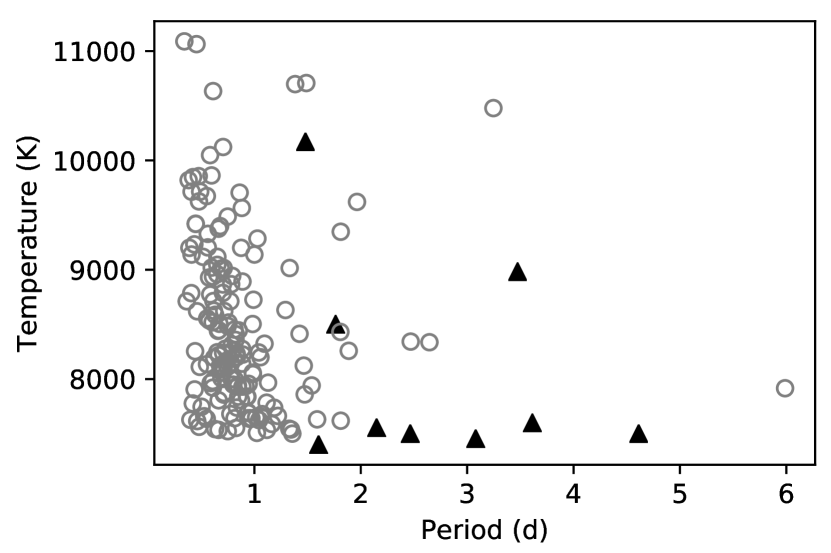
Figure 1: Black triangles: detected and confirmed planets of A-type stars. Gray circles: additional possible planets according to Balona 2014 (see exoplanet.eu).

2 RV-measurements

Balona (2014) analysed the light curves of 1974 A-type stars obtained with the Kepler satellite (Borucki et al., 2010). They found peculiar features in the periodograms of 166 of them. The peculiar feature consists of a broad peak (possibly due to differential rotation) and a sharp feature at a slightly higher frequency. Balona (2014) claim that the sharp feature could be caused by a planet with a similar orbital period as the rotational period.

Since Balona (2014) interpret the peculiar feature as a result of the beaming and ellipsoidal modulations (Mazeh & Faigler, 2010), the object causing this would have to be a massive hot Jupiter, or a brown dwarf, or even low-mass stellar companion (Tal-Or et al., 2015). This hypothesis can thus be tested by obtaining RV-measurements with meter-class telescopes. However, A-type stars are usually rapidly rotating and have only few spectral lines. The expected RV-error is proportional to the $v$ sin $i$ of the star. Therefore, the expected RV precision is 20-60 times lower than for a comparable G-type star (Hatzes, 2016). One way to deal with the lower RV precision is to take a lot of measurements. For example, we required 248 RV-measurements to determine the mass of WASP-33b (Lehmann et al., 2015), which has a K-amplitude of around 300 m s^-1.

By selecting a number of stars from this list and obtaining several tens of RV measurements of each one, we can put first constrains on the masses of potential companions. Therefore, we randomly selected a small subsample of six stars that were observed with the 2-m telescopes in Tautenburg and Ondřejov. An overview of the properties of this subsample is provided in Table 1.

Table 1: The sample

name	$\alpha$ (J2000.0)1	SpT2	$m_{\text{v}}^{3}$	parallax1
other name	$\delta$ (J2000.0)1			(mas)
KIC 3766112	19${}^{\text{h}}$44${}^{\text{m}}$1.9${}^{\text{s}}$	A0	11.3	$0.92\pm 0.04$
HD 225570	+38∘52′58.5′′
KIC 4944828	19${}^{\text{h}}$47${}^{\text{m}}$47.2${}^{\text{s}}$	A5	9.9	$2.04\pm 0.03$
HD 225856	+40∘0′57.3′′
KIC 7352016	19${}^{\text{h}}$13${}^{\text{m}}$14.2${}^{\text{s}}$	A9	12.0	$1.15\pm 0.02$
TYC 312925431	+42∘54′49.5′′
KIC 7777435	19${}^{\text{h}}$55${}^{\text{m}}$24.4${}^{\text{s}}$	A2	10.7	$1.39\pm 0.03$
HD 188874	+43∘29′48.0′′
KIC 9222948	19${}^{\text{h}}$34${}^{\text{m}}$46.7${}^{\text{s}}$	A1	10.2	$2.25\pm 0.05$
BD+45 2925	+45∘37′11.8′′
KIC 9453452	19${}^{\text{h}}$4${}^{\text{m}}$36.1${}^{\text{s}}$	A4	10.6	$1.57\pm 0.03$
TYC 354130011	+46∘3′37.9′′

¹ Taken from Gaia DR2 (Gaia Collaboration et al., 2016, 2018)
² Taken from Frasca et al. (2016)
³ Taken from Høg et al. (2000)

2.1 Data obtained with the Alfred-Jensch 2-m telescope at Tautenburg observatory

The sample of six A-type star planet candidates was monitored with the 2-m Alfred Jensch telescope of the Thüringer Landessternwarte Tautenburg which is equipped with an echelle spectrograph with resolving power of $\lambda/\Delta\lambda=35000$ with the two arsec slit used. We observed MASCARA-1 b as a reference object, because it is an A-type star with a known planet.

The typical signal to noise of the obtained spectra is listed in Table 2:

Table 2: Typical S/N of the Tautenburg observations

star	S/N	star	S/N
KIC 3766112	25 – 45	KIC 7777435	30 – 60
KIC 4944828	40 – 80	KIC 9222948	40 – 75
KIC 7352016	30 – 35	KIC 9453452	30 – 60
MASCARA-1	80 – 120

The data-reduction followed the usual steps, bias-subtraction, flat-fielding, removal of Cosmic Rays, scattered light subtraction, extraction, wavelength calibration and normalization. All methods were combined using the Tautenburg Spectroscopy Pipeline – $\tau$-spline. The pipeline makes use of standard IRAF and PyRaf routines and the Cosmic Ray code by Malte Tewes based on the method by Van Dokkum (2001).

We used the telluric lines in order to account for instrumental shifts. The telluric shift was obtained by cross correlation of a telluric O₂-template (extracted with the ESO Program Molecfit, see Smette et al. (2015) and Kausch et al. (2015)) with the object spectra.

2.2 Data obtained with the Perek 2-m telescope at Ondřejov observatory

The advantage of a monitoring network of telescopes at central Europe is that we can obtain a better coverage of the data sets. Therefore, we also used Perek 2-m telescope located at the Astronomical Institute of the Czech Academy of Sciences at Czech Republic. It is equipped with an Echelle Spectrograph (OES).

OES has resolving power $\lambda/\Delta\lambda=44000$ and a slit width of 0.6 mm, corresponding to 2 seconds of arc on the sky. Further details and description of instrument capability can be found in (Kabáth et al., 2019).

We monitored the same sample of stars as Alfred-Jensch telescope as described in Tab 1. The data was reduced in the same way as described in Section 2.1 for the Tautenburg data. To obtain a higher signal to noise 2-3 spectra were combined.

The typical signal to noise of the obtained spectra is listed in Table 3:

Table 3: Typical S/N of the Ondřejov observations

star	S/N	star	S/N
KIC 4944828	20 – 30	KIC 9222948	20 – 40
KIC 9453452	15	MASCARA-1	35

2.3 Results of the RV-measurements

The radial velocities were obtained by cross correlation. The template was obtained by co-adding all spectra of the star similar to the method described in Anglada-Escudé & Butler (2012). We obtained the RV error for each spectrum by cross correlating every order separately. After removing outliers we use the mean value as radial velocity and the standard deviation as the corresponding error.

The resulting RV values were analysed with the Radial Velocity Modeling Toolkit – RadVel – by Fulton et al. (2018). This algorithm uses a simple maximum-likelihood fit as an initial guess and afterwards performs a Markov-Chain Monte Carlo (MCMC) exploration to obtain the corresponding errors. The starting values for the fit are the periods published by Balona (2014) and we assume zero eccentricity as the planets are supposedly close-in.

We have observed MASCARA-1 b as a reference object to make sure that with our method we are capable of measuring masses of hot Jupiters around A-type stars. We used exactly the same method as for the other stars. We took 114 measurements in Tautenburg and analysed them in the same way as described above. We obtain a K-amplitude of 391,m s^-1 $\pm$ 130 m s^-1 (see Fig. 2) which is consistent with the K-amplitude reported by Talens et al. (2017) of 400 m s^-1 $\pm$ 100 m s^-1.

As we do not have as many observations for the ’Balona stars’, we will only obtain upper limits for the possible planet masses. To obtain the upper limits we use the fitting algorithm of RadVel with a high initial K-amplitude value. The K-amplitude of the initial fit can be used as an estimate of the upper limit similar to what (Talens et al., 2018) did.

To show how this works we reduce the number of measurements of MASCARA-1 b randomly to 30 which is in the order of magnitude of the measurements we obtained for the ’Balona stars’. Still we can fit a radial velocity curve to the data. The result is shown in Fig. 3. The K-amplitude in this example is 570 m s^-1 which matches the upper value obtained from the MCMC algorithm we ran on the whole set of measurements. Running RadVel’s MCMC algorithm now gives zero as the most probable K-amplitude.

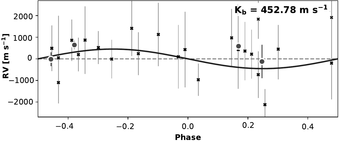
Figure 10: RV curve of KIC 3766112

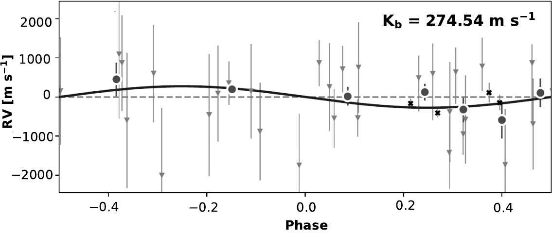
Figure 14: RV curve of KIC 9453452

All six RV-curves of the ’Balona-stars’ can be fitted with a simple maximum-likelihood fit as well. As soon as we run the MCMC algorithm the K-amplitudes turn out to be not significant (see e.g. Fig. 4). We therefore use the K-amplitude of the initial fit and the known stellar masses to obtain upper limits for the possible companion masses with 1 $\sigma$ confidence. The upper limits with 99 per cent confidence range from 3.8 M${}_{\text{Jup}}$-7.3M${}_{\text{Jup}}$ and are summarised in Table 4. The similar upper limits are not surprising as the variations are most probably only due to measurement errors. We obtained a similar amount of measurements for each star and a similar S/N for the individual spectra. Therefore instrumental effects would necessarily lead to similar results. All other radial velocity curves are reported in the appendix (Fig. 10, 11, 12, 13 and Fig. 14).

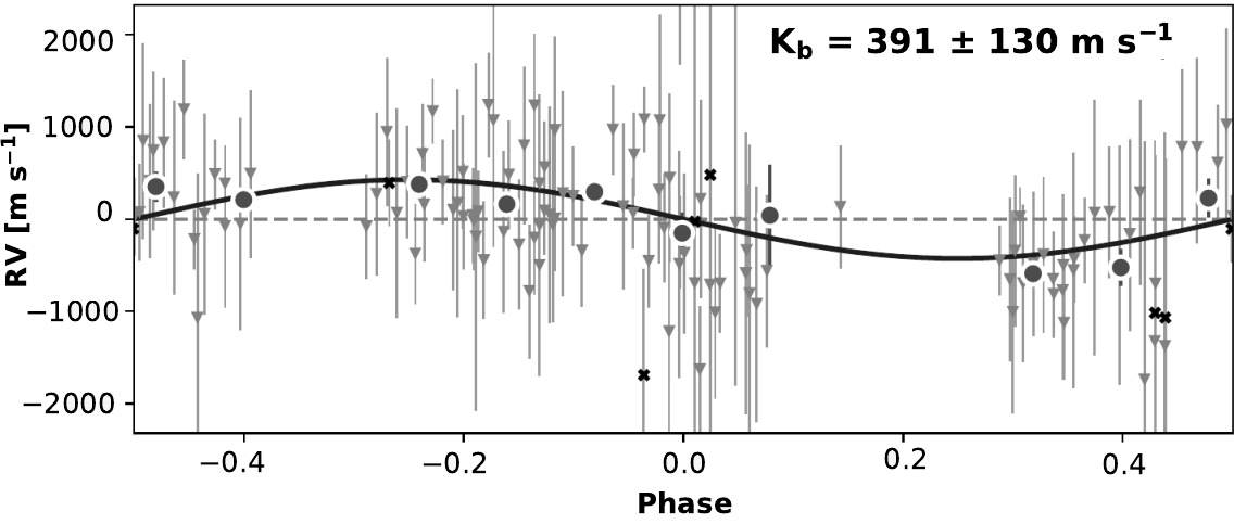
Figure 2: RV curve for MASCARA-1 b. X: the Ondřejov values; Triangles: the Tautenburg values; Circles: Binned radial velocities

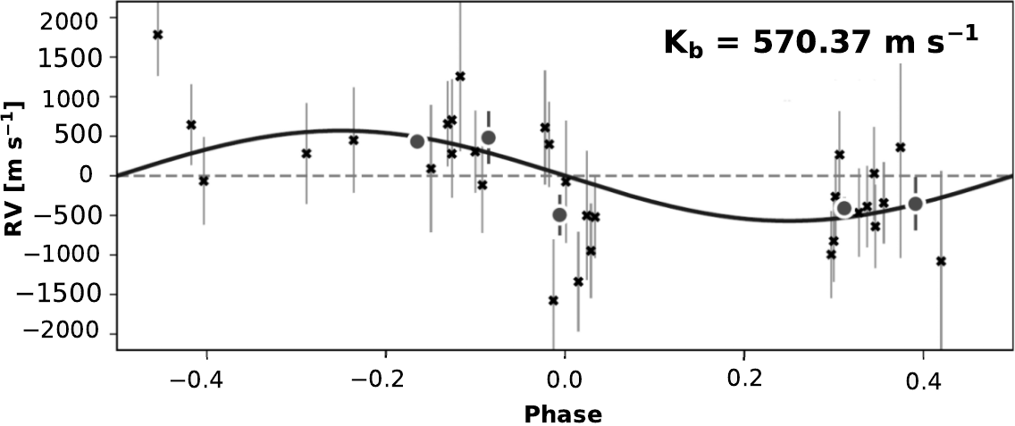
Figure 3: Example of upper limit for MASCARA-1 b with only 30 data points from Tautenburg, black curve is the maximum-likelihood fit

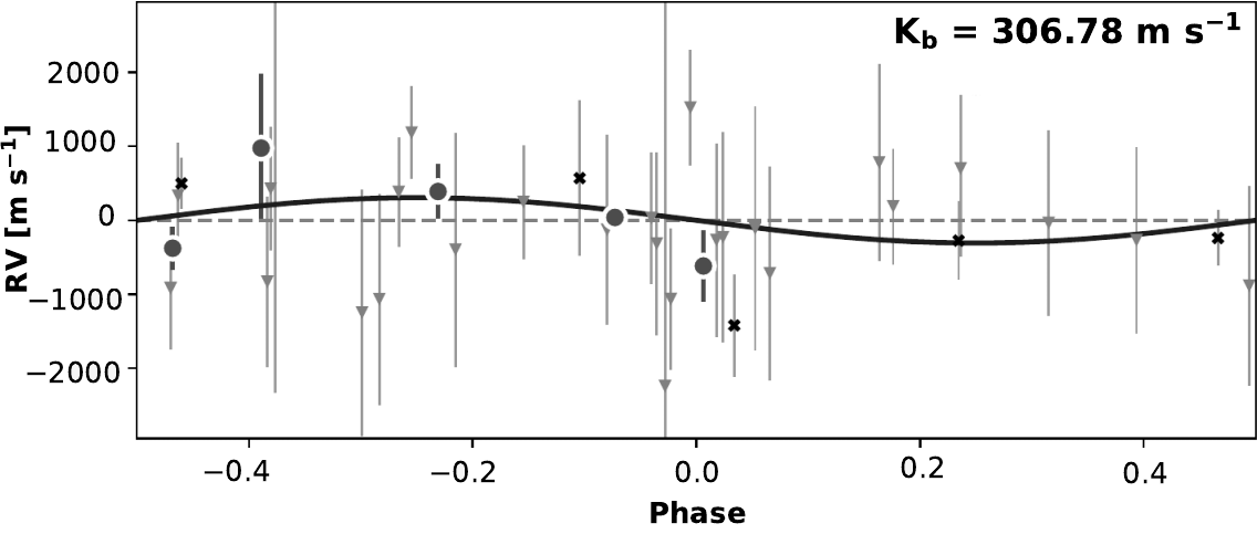
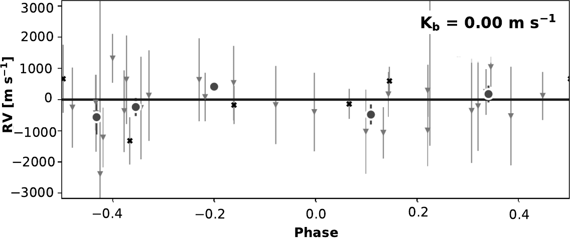
Figure 4: RV curve of KIC 9222948; upper panel: simple maximum-loglikelihood fit to the data; lower panel: most probable K-amplitude after MCMC

star	star mass	max. K	period	upper limit
	(M⊙)	(ms-1)	(d)	(M${}_{\text{Jup}}$)
KIC 3766112	2.2	450	0.45	7.3
KIC 4944828	2.0	330	0.93	6.3
KIC 7352016	3.0	290	0.93	7.3
KIC 7777435	2.1	210	0.68	3.8
KIC 9222948	2.3	310	1.29	7.3
KIC 9453452	2.1	270	0.61	4.5

Table 4: Summary of the upper limits.

3 Transit Analysis

The possible planets published by Balona (2014) should all have relatively short periods and large radii. This makes it obvious to look for transits.

From the average stellar radius $R_{\text{star}}\approx$ 2.3 $R_{\odot}$ and the typical orbital radius $a\approx$ 0.02 au (Balona, 2014) we can calculate the transit probability $P_{\text{transit}}=\frac{R_{\text{star}}}{a}$ of every single ’possible planet’. It is around 53 per cent. Therefore, the probability that all 166 possible planets are not transiting is as low as 10^-55. Balona (2014) argues that the transits could be overlooked because the transit takes a big part of the orbit and because it could be hidden in the activity.

We therefore decided to model the transits in the light curves and see if we can retrieve them with the transit finding pipeline EXOTRANS (Grziwa et al., 2012; Korth et al., 2019).

The possible planets need to have at least the mass and radius of Jupiter. This is because the ellipsoidal-, beaming- and reflection effects are mass and radius dependent (Mazeh & Faigler, 2010; Faigler & Mazeh, 2011). In Fig. 6 we show a simple model of the three effects for a Jupiter-like planet. The figure shows that it is possible to retrieve the amplitude of the light curve variations due to a none transiting companion. In Fig. 6 we show one example of a phase-folded light curve of KIC 9222948. From this we know that we cannot retrieve the shape of the light curve with the model. This could be due to an overlap with an effect on the star, e.g. spots, oscillations, pulsations.

We list the expected transit depths of the six stars we have analysed in Section 2.3 for 1 R${}_{\text{Jup}}$ size planets in Table 5.

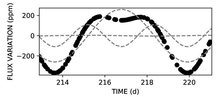
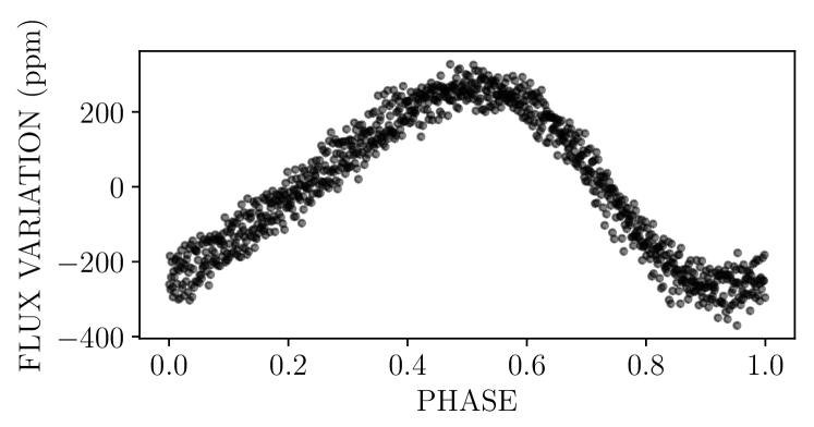
Figure 5: Model of ellipsoidal-, beaming- and reflection effect. Dashed lines: single effect, dotted line: combined effects

Figure 6: Light curve of KIC 9222948, phase-folded with the period from Balona (2014) and binned

To model the transit we used the actual light curves and combined them with a transit model. This model was obtained by using the code of Parviainen (2015) with the radii obtained from Berger et al. (2018) and the limb darkening coefficients from Sing (2010). In Fig. 7, we show one model transit of a Jupiter size object in a Kepler light curve. All modeled transits can be easily retrieved by the detection software.

We consequently ran the transit finding algorithm on all 166 A-type stars and could not detect a single transit event from a Jupiter-like planet. All detected signals were much too small for a Jupiter like transit and were most likely activity signals.

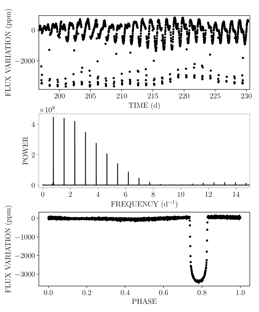
Figure 7: Transit model of a Jupiter size object in Kepler light curve of KIC 9222948; top panel: 30 d section of the time series, middle panel: periodogram of the light curve, lower panel: phase-folded and binned light curve

Table 5: Summary of the expected transit depth.

star	Period (d)	R${}_{\text{star}}$ ($R_{\odot}$)	Transit depth if
			R${}_{\text{p}}\approx$ R${}_{\text{Jup}}$
KIC 3766112	0.45 d	2.3201	0.19 %
KIC 4944828	0.93 d	2.4571	0.17 %
KIC 7352016	0.93 d	2.0731	0.23 %
KIC 7777435	0.68 d	2.5721	0.15 %
KIC 9222948	1.29 d	1.8211	0.30 %
KIC 9453452	0.61 d	2.1661	0.21 %

¹ Taken from Berger et al. (2018)

4 Hot Jupiter Frequency with Kepler Analysis

The Kepler satellite observed around 2000 A-type stars (Brown et al., 2011). It found exactly one transiting hot Jupiter around A-type stars (Kepler-13 A b). There are three other confirmed candidates:

• Kepler-340 b with an orbital period of 22.9 d and a size of 3.36 R_⊕,

• Kepler-340 c with an orbital period of 14.8 d and a size of 2.49 R_⊕,

• Kepler-1115 b with an orbital period of 23.5 d and a size of 1.7 R_⊕.

None of them can be classified as a hot Jupiter. The only other KOI around A-type stars with orbital periods less than 10 d are KOI 80, KOI 971, KOI 6068, KOI 7733 and have planet sizes of 96 R_⊕, 134 R_⊕, 100 R_⊕ and 4.5 R_⊕ respectively. Therefore, none of these objects is likely to be classified as a hot Jupiter later. KIC 11180361 or KOI 971 is also in the sample of Balona (2013) and can be classified as a binary system with the output of EXOTRANS. KOI 80 and KOI 6068 are more likely to be binary stars as well, considering their transit depth.

Assuming a high occurrence rate of hot Jupiters of around 1.2 per cent, there should be a around 26 hot Jupiters in the whole sample. Even assuming that they are so close that the transit probability is around 50 per cent, there should be only around 13 transiting hot Jupiters in the sample. Taking the lower value of 0.15 per cent only three hot Jupiters should be in the sample of which one or two would be transiting. For a planet orbiting its star in a 10 days orbit instead of a 1 day orbit (about 0.09 au), the transit probability drops as low as 11.5 per cent. In this case three or less transits should be present for the whole Kepler sample.

To obtain a more quantitative statement on the expected number of transits we conduct a small simulation. We take the actual stellar radii of the whole Kepler A-star sample from Berger et al. (2018) – around 2000 stars. We assign each of them a planet with a certain probability (8.4 per cent for a planet frequency of 8.4 per cent). Then this planet gets a random semimajor axis between 0.01 au and 0.1 au. From this we calculate the transit probability $P_{\text{transit}}=\frac{R_{\text{star}}}{a}$. Then we randomly draw a 1 or a 0 with exactly this probability – equal to throwing a coin that shows ’transit yes’ or ’transit no’. Then we count all the transits. We repeat this process 7000 times. After all 7000 simulations are finished, we obtain a number of simulations that show a certain number of transits. This number we translate to a probability density by normalization.

To obtain a range of transits we would expect for different planet frequencies, we take the 2 $\sigma$-range of the probability densities (or more precisely the 95 per cent values around the median value) – see Fig. 8. For a frequency of 0.15 per cent as predicted by Stephan et al. (2018) we therefore expect 0-3 transits and for a frequency of 1.2 per cent we expect 4-15 transits. Therefore, the lower frequency is much more likely.

This raises the question whether we can find an upper limit for the giant planet frequency around Kepler A-type stars. To obtain an estimate of the upper limit we increase the planet frequency of our simulation until the expected number of transits is at least 2. This is the case for a planet frequency of about 0.75 per cent (2-10 transits). This is a rather conservative upper limit considering that 1 $\sigma$ or 68 per cent of all values already lead to an estimate of 3-8 transits.

If all ’possible planets’ were indeed planets (planet frequency of 8.4 per cent) we would expect 49-78 transiting planets.

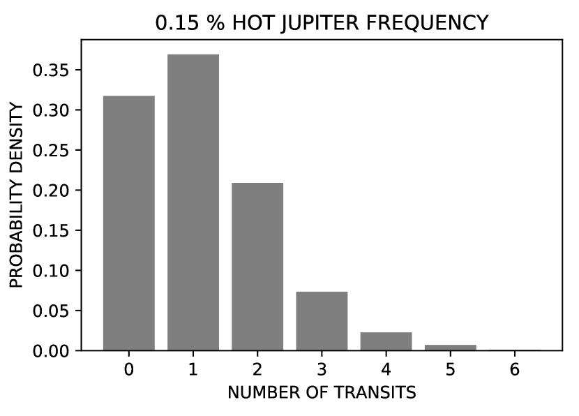
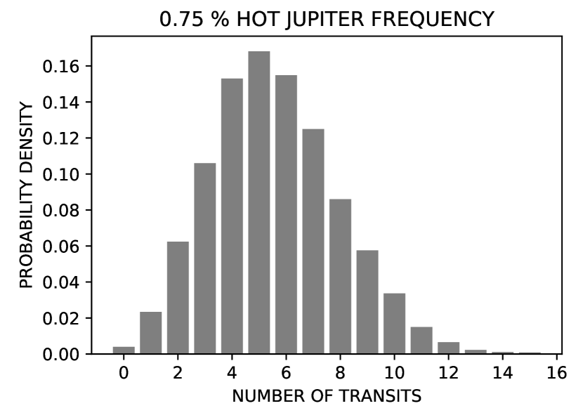
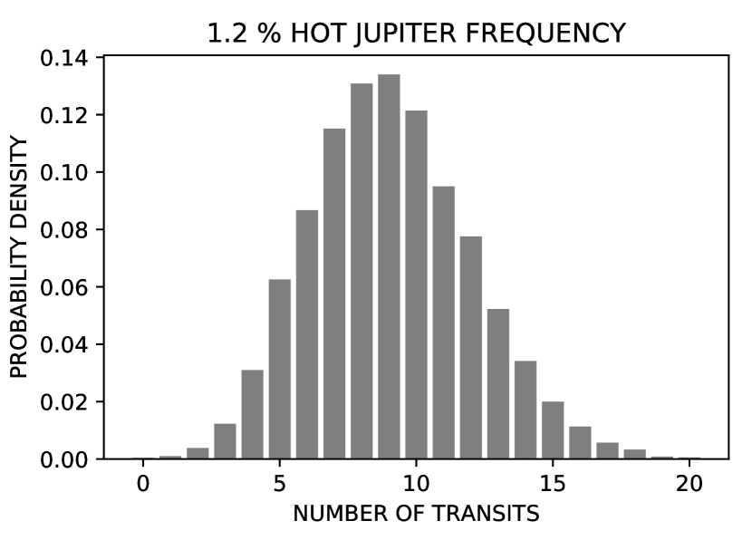
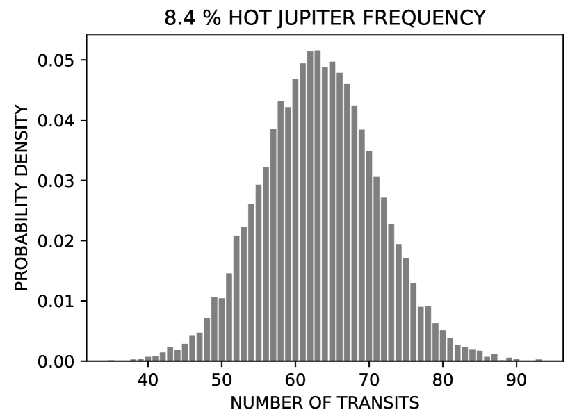
Figure 8: Transiting objects expected for different planet frequencies with 2 $\sigma$; 0.15 per cent 0-3 Transits (1 $\sigma$: 0-2 transits), 1.2 per cent 4-15 Transits (1 $\sigma$: 6-12 transits), 0.75 per cent 2-10 Transits (1 $\sigma$: 3-8 transits), 8.4 per cent 49-78 Transits (1 $\sigma$: 55-71 transits)

5 Discussion

Combining the results from above a very high hot Jupiter frequency of 8.4 per cent (as in Balona (2014)) seems very unlikely for several reasons:

• a transiting hot Jupiter shows up in the Lomb-Scargle periodogram of a light curve – it therefore should be easily detected,

• the Kepler team and pipeline must have missed around 130 transiting objects,

• we derive an upper limit on the hot Jupiter occurrence rate from Kepler light curves of 0.75 per cent,

• the CoRoT survey found evidence that the number of hot Jupiters is similar for A-type and G-type stars and

• an upper limit on the occurrence rate of 4.5 per cent was determined on a sample of A-type stars observed with HARPS and SOPHIE.

In this section we explain our reasoning in more detail.

Kepler-13 A b is a Jupiter size planet that was discovered by Shporer et al. (2011). In Fig. 9 we show the periodogram of its light curve. It becomes obvious that the rotation period of the star could not be retrieved without first subtracting the transits. This could be one reason why Kepler-13 A b does not show up in the sample of Balona (2013).

We double checked this assumption with our transit blind tests (see Fig. 7) and can confirm that the transiting signal becomes the dominant feature in the periodogram for all hot Jupiters. In the 2013 sample there are two Kepler planets (Kepler-340 b&c and Kepler-1115 b). In those two examples the rotation period is very different from the candidate period such that the rotational peak can still be retrieved.

This means that the selection pattern used to describe the A-star activity in periodograms would exclude all transiting hot Jupiters. Nevertheless, if all 166 planets actually exist and all of them were found in Balona (2014) this means that, as a maximum, exactly the 66 per cent non-transiting planets were selected. The planet frequency would therefore not only be as high as 8.4 per cent but as high as 12.6 per cent. This means that the remaining around 1800 stars should show around 130 transiting hot Jupiters. The fact that by the Kepler pipeline itself only one example of a transiting hot Jupiter was found makes it very improbable that 129 transiting planets were overlooked until now. This scenario is unlikely given that Kepler-13 A b was easily detected.

In the CoRoT survey, Guenther et al. (2016) found 9 candidates for planets of A-type stars. Three of them are binaries, one is a brown dwarf. Using AO-imaging and NIR spectroscopy they could exclude that they are false-positives. Using spectroscopy obtained with UVES they obtained upper limits of their masses which are all in the planetary regime. Assuming that these candidates are hot Jupiters, the number of hot Jupiters is the same for A-type as for G-type stars (Guenther et al., 2016). With an occurrence rate of 8.4 per cent instead of $\approx$ 1.2 per cent the frequency of hot Jupiters were about 7 times larger for A-type stars than for G-stars. Consequently, they would have found 7 times as many candidates, because the photometric sensitivity of CoRoT was more than sufficient to detect hot Jupiters of A-type stars. The CoRoT survey thus shows that the frequency of hot Jupiters of A-type stars is about the same, or even less than that of G-stars. The CoRoT survey thus also excluded that the frequency of hot Jupiters of A-type stars is as high as 8.4 per cent.

Although RV-surveys of A-type stars are very challenging, Borgniet et al. (2019) calculated the occurrence rate of close-in BD and giant planets from their sample with HARPS and SOPHIE. They concluded that the giant planet occurrence rate is lower than 4.5 per cent. In this paper we show that Kepler retrieves an upper limit on the close-in hot Jupiter occurrence rate of 0.75 per cent. Combining the absence of transits in the Kepler sample of A-type stars and our upper limits a very high hot Jupiter frequency of 8.4 per cent seems very unlikely.

When compared to the theoretical predictions of the hot Jupiter frequency around main-sequence A-type stars our results are more consistent with the lower end of predictions like the ones from Stephan et al. (2018).

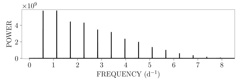
Figure 9: Periodogram of Kepler-13 A b

Nevertheless the question remains open what else could be the cause of the peculiar feature.

Although we find only upper limits in the range of 1.5-2.9 M${}_{\text{Jup}}$, we can disprove the hypothesis that a close stellar companion is the source of the strange feature in the periodogram. A stellar companion would need to have an orbit of more than 30 years such that we could not find its trend in our two years of data. Due to Kepler’s lower spacial resolution, a stellar companion in an orbit of up to 1000 years could still be present in the same Kepler pixel.

Saio et al. (2018) propose a different explanation for the broad and sharp feature in the periodogram. They suggest that the sharp feature could be a signature of spots on the star. The broad feature could then be explained by Rossby waves. They explain that there should be a link between the rotational frequency and that of the Rossby waves. Therefore they call those stars with the peculiar feature ’hump & spike’ stars. Nevertheless the question remains open why some of the rapidly rotating A-type stars show this kind of oscillations and some do not. In fact, in 81 per cent of the original Balona (2013) sample this kind of oscillations are not triggered.

The hypothesis of Saio et al. (2018) could be tested by taking a time series of spectra of the brightest targets of the sample. If the line distortions match the two periods causing the broad and the sharp peak this could indicate the presence of spots and oscillations. An exoplanet on the other hand does not cause line distortions that match its orbital period. This test was beyond the scope of this work and still needs to be conducted in the future.

Another explanation according to Sikora et al. (2018) could be that the sharp peaks originate from inhomogeneities near the surface and the broad peaks in a region near a convective-radiative boundary, but their studies are still ongoing.

6 Conclusions

Aim of this work is to compare theories of planet formation and evolution with observations. Jupiter-sized planets around intermediate-mass main-sequence stars are still very rare. Theories predict either a high frequency of close-in Jupiter-like planets around these stars (> 1.2 per cent) or a very low frequency (0.15 per cent).

Balona (2014) found peculiar features in light curves of 166 Kepler stars. One possible explanation for this feature is the presence of close-in Jupiter sized companions. If these features are in fact the signature of close-in, massive planets it would mean that the frequency of such planets is a as high as 8 per cent. This is significantly higher than theories predict.

With observations from our two 2-m telescopes in Ondřejov and Tautenburg we present upper limits of possible planetary-companion masses in the range of 3.8 M${}_{\text{Jup}}$-7.3 M${}_{\text{Jup}}$ for six of the stars in question. This excludes close-in stellar companions as well as planets that are heavier than 7.3 M${}_{\text{Jup}}$.

We confirm that none of the planet candidates is transiting although statistically there should be around 80 transits. This makes the hypothesis of the 166 planets very unlikely.

From the Kepler sample of A-type stars there is only one detection of a hot Jupiter. As we have shown, transiting planets with the size of Jupiter can easily be detected in the Kepler data, even if they orbit A-type stars.

We derive that there is an upper limit of hot Jupiters of about 0.75 per cent. This is most consistent with the lower end of theoretical predictions.

This is evidence for a lack of hot Jupiters around intermediate-mass main-sequence stars.

Appendix A Radial Velocities

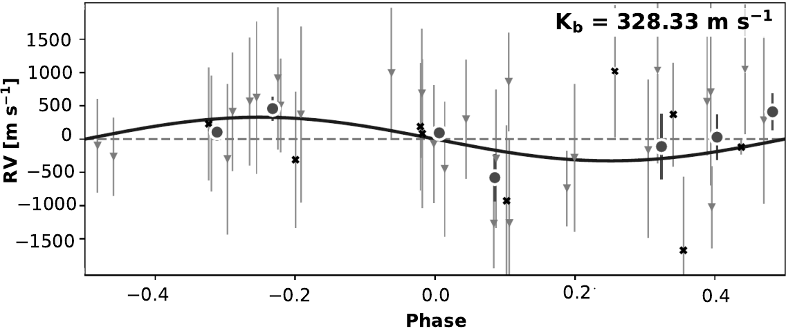
Figure 11: RV curve of KIC 4944828

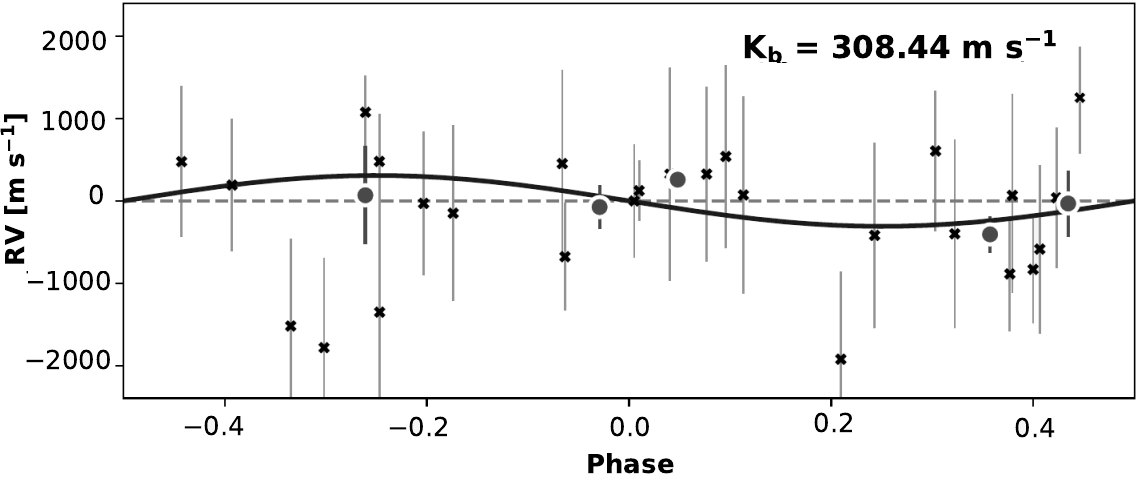
Figure 12: RV curve of KIC 7352016

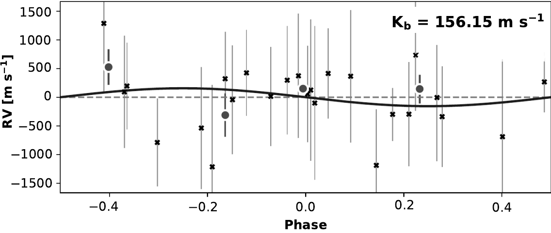
Figure 13: RV curve of KIC 7777535

	MASCARA-1-b Tautenburg data
time	rv	rv err	time	rv	rv err
(bjd)	($\frac{\text{m}}{\text{s}}$)	($\frac{\text{m}}{\text{s}}$)	(bjd)	($\frac{\text{m}}{\text{s}}$)	($\frac{\text{m}}{\text{s}}$)
+2450000			+2450000
7966.36	2103	874	7980.35	2402	303
7966.39	2101	1027	7980.38	2393	1133
7966.43	1931	608	7980.4	1766	898
7966.46	1349	382	7980.42	1071	468
7966.47	1395	493	7980.46	1539	1061
7966.49	1735	820	7979.53	1244	859
7971.39	1494	1223	7980.55	983	694
7971.4	1833	591	7980.57	401	1265
7971.42	1363	484	7980.59	761	808
7971.43	1404	404	7995.33	2291	455
7971.45	2559	538	7995.35	1460	882
7971.46	2393	1360	7995.37	1389	338
7971.48	1185	863	7995.4	867	470
7971.49	1802	565	7995.42	1637	770
7971.53	539	704	7995.43	1225	566
7971.54	2554	758	7995.44	102	1260
7971.55	820	1189	7995.46	834	1219
7971.57	1370	1163	7995.47	953	851
7971.58	2285	1002	7995.49	628	633
7971.56	1885	465	7995.5	-309	662
7972.45	873	334	7995.52	611	1003
7972.47	667	869	7995.53	309	916
7972.48	978	799	7995.54	624	505
7972.49	1345	267	7995.57	1281	1758
7971.51	1046	683	7995.59	734	1520
7971.52	2120	836	7996.37	-418	2582
7971.54	1119	584	7996.39	-3	2173
7971.55	1709	945	7996.41	-54	2306
7971.56	1412	443	7998.34	670	489
7971.58	1328	536	7998.36	821	754
7971.55	1253	1104	7998.38	768	1266
7973.36	1242	539	7998.45	1397	692
7973.38	1594	864	7998.47	825	1287
7973.4	2265	780	7998.49	1159	1032
7973.42	1389	1125	7998.51	1612	989
7973.44	1725	580	7998.54	621	1372
7973.47	2027	510	7999.36	1129	1874
7973.49	2488	303	7999.51	1262	1040
7973.51	1728	425	7999.53	1603	1099
7973.53	1421	849	7999.55	1572	507
7973.55	1350	546	8000.41	315	1087
7973.57	1306	506	8000.43	626	834
7973.59	877	613	8000.45	840	762
7979.34	2343	1029	8000.47	937	828
7979.37	2170	1046	8000.49	508	437
7979.39	2065	844	8000.51	197	592
7979.41	2152	682	8000.53	891	432
7979.43	1557	1037	8000.55	1091	426
7979.45	2510	512	8000.57	1388	1534
7979.47	1102	270	8001.39	945	514
7979.49	1376	1076	8004.37	1454	643
7979.51	1806	337	8007.41	251	1559
7979.53	1706	353	8008.49	513	1610
7979.56	1521	736	8012.46	979	580
7979.58	1812	892	8013.4	549	952
7979.56	1268	1140	8014.3	1479	592
7980.33	2020	421

Table 6: Barycentric Julian dates at mean exposure and the radial velocities determined from cross-correlation.

MASCARA-1-b Ondřejov data
time	rv	rv err
(bjd)	($\frac{\text{m}}{\text{s}}$)	($\frac{\text{m}}{\text{s}}$)
+2450000
8313.41	791	1156
8313.48	5211	1054
8313.51	2453	2798
8313.54	2959	3167
8313.59	6032	3331
8314.56	2375	364
8314.41	1465	1712
8314.43	1412	1729
8334.4	2874	473

Table 7: Barycentric Julian dates at mean exposure and the radial velocities determined from cross-correlation.

KIC 3766112			KIC 4944828
time	rv	rv err	time	rv	rv err
(bjd)	($\frac{\text{m}}{\text{s}}$)	($\frac{\text{m}}{\text{s}}$)	(bjd)	($\frac{\text{m}}{\text{s}}$)	($\frac{\text{m}}{\text{s}}$)
+2450000			+2450000
		Tautenburg
7557.49	-469	1402	7557.51	942	982
7558.46	74	1080	7558.51	-499	1016
7562.48	-1348	569	7562.51	970	1384
7563.49	-909	1604	7563.51	653	1396
7564.48	-976	1159	7564.51	232	1254
7566.51	-815	316	7585.49	246	897
7592.39	-1121	895	7585.53	-344	1039
7585.47	-1098	711	7588.52	-217	1315
7588.5	-1292	1818	7625.41	-122	887
7625.39	-848	801	7625.41	-122	887
7625.39	-848	801	7880.47	1000	976
7883.51	-366	1144	7883.53	515	962
7884.48	-889	1219	7884.5	454	704
7889.51	576	2206	7889.45	810	744
7911.45	798	989	7911.42	572	1146
7918.5	-209	1294	7918.53	-1075	620
7924.47	-910	1675	7923.47	360	892
7940.42	-477	656	7923.53	864	1073
7944.45	-2435	666	7924.49	320	1326
8001.46	-3458	207	7940.45	636	972
8008.38	-1139	348	7944.36	-790	569
8009.43	-1241	1297	7944.37	-332	1109
8012.36	-1535	1532	8001.53	-351	1132
8013.51	-2304	263	8007.46	-1321	675
8014.5	-2067	829	8008.41	-1314	1270
			8012.39	510	805
			8012.51	-149	705
			8014.39	-315	590
			8014.52	33	871
		Ondřejov
			7884.52	-279	1023
			7892.47	-1641	1105
			7905.39	1051	994
			7926.51	113	1120
			7929.41	-896	1135
			7935.52	260	849
			7946.36	402	787
			8314.48	-89	111
			8334.5	220	959

Table 8: Part 1: Barycentric Julian dates at mean exposure and the radial velocities determined from cross-correlation.

KIC 7352016			KIC 7777435
time	rv	rv err	time	rv	rv err
(bjd)	($\frac{\text{m}}{\text{s}}$)	($\frac{\text{m}}{\text{s}}$)	(bjd)	($\frac{\text{m}}{\text{s}}$)	($\frac{\text{m}}{\text{s}}$)
+2450000			+2450000
		Tautenburg
7557.42	-325	1115	7557.53	206	977
7558.42	-653	303	7558.52	479	1154
7562.41	-172	951	7562.53	238	1235
7563.41	-711	1164	7563.53	380	531
7564.38	-740	829	7564.53	410	943
7566.41	-585	775	7585.51	128	864
7589.43	-1664	666	7588.42	846	968
7585.40	-454	1278	7588.54	-574	1348
7588.45	-1176	1129	7625.43	69	951
7625.33	-778	657	7883.55	435	815
7625.52	-2699	1042	7884.52	108	1112
7880.49	-300	891	7889.48	1400	1186
7883.46	-298	538	7911.47	528	785
7884.43	-808	847	7919.44	-1099	1427
7884.56	-1454	618	7923.49	-423	1062
7914.43	-452	1040	7924.50	-225	877
7919.42	475	643	7940.49	538	747
7923.41	298	392	7944.39	309	759
7924.42	-926	1048	8001.55	170	842
7940.47	-239	1095	8007.44	-674	765
7944.47	-1608	617	8008.42	-1073	975
8001.49	-2128	1345	8012.40	12	1339
8008.33	-706	1178	8012.53	-182	910
8009.38	-1196	1111	8014.41	486	1082
8012.32	-1363	1003	8014.54	-185	463
8013.49	-2296	1035
8014.45	-2559	1071

Table 9: Part 2: Barycentric Julian dates at mean exposure and the radial velocities determined from cross-correlation.

KIC 9222948			KIC 9453452
time	rv	rv err	time	rv	rv err
(bjd)	($\frac{\text{m}}{\text{s}}$)	($\frac{\text{m}}{\text{s}}$)	(bjd)	($\frac{\text{m}}{\text{s}}$)	($\frac{\text{m}}{\text{s}}$)
+2450000			+2450000
		Tautenburg
7557.44	-668	893	7557.40	-13	1176
7558.44	-316	737	7558.39	-461	1197
7562.46	-450	771	7562.38	256	1553
7563.46	-272	836	7563.38	148	1144
7564.46	-968	1265	7564.41	-1069	1557
7566.49	-1014	1236	7566.38	-350	1111
7590.43	-1583	1348	7568.39	174	609
7585.42	-1530	1150	7585.35	-2035	911
7588.47	-1763	956	7585.37	-1182	1117
7625.36	-1614	825	7625.31	-1147	442
7625.36	-1614	825	7625.31	-1147	442
7880.52	-927	1419	7880.44	28	800
7883.48	-734	1257	7883.43	-124	832
7884.45	-1416	1451	7884.41	-251	527
7889.43	-827	1288	7884.54	-1155	736
7911.49	823	787	7889.54	-992	1270
7912.46	485	627	7912.48	105	571
7919.46	82	1328	7919.49	484	1641
7923.43	0	1196	7923.38	263	565
7924.44	-966	1310	7924.39	-9	1235
7941.44	-511	781	7939.53	262	1212
7944.49	-366	714	7941.47	-519	1215
8001.57	-1764	1428	7942.38	-1558	496
8008.36	-2940	7302	7942.49	-456	1362
8009.41	-1095	1583	8001.51	-2615	1720
8012.34	-809	1645	8008.31	-1489	1240
8014.37	2635	5670	8009.36	-1207	1720
8014.47	-1946	1670	8012.29	-1302	1153
			8013.47	-2342	1423
			8014.43	-2357	1313
		Ondřejov
7892.42	-366	415	7891.41	251	254
7929.45	476	993	7928.46	-3	199
7948.37	405	69	7948.42	-268	115
7995.52	-1512	606	8322.40	-25	126
8334.58	-332	167

Table 10: Part 3: Barycentric Julian dates at mean exposure and the radial velocities determined from cross-correlation.

References

- Alibert et al. (2011) Alibert Y., Mordasini C., Benz W., 2011, A&A, 526, A63
- Anderson et al. (2016) Anderson K. R., Storch N. I., Lai D., 2016, Monthly Notices of the Royal Astronomical Society, 456, 3671
- Anderson et al. (2018) Anderson D., et al., 2018, arXiv preprint arXiv:1809.04897
- Anglada-Escudé & Butler (2012) Anglada-Escudé G., Butler R. P., 2012, ApJS, 200, 15
- Balona (2013) Balona L., 2013, Monthly Notices of the Royal Astronomical Society, 431, 2240
- Balona (2014) Balona L., 2014, MNRAS, 441, 3543
- Berger et al. (2018) Berger T. A., Huber D., Gaidos E., van Saders J. L., 2018, ApJ, 866, 99
- Borgniet et al. (2019) Borgniet S., et al., 2019, Astronomy & Astrophysics, 621, A87
- Borucki et al. (2010) Borucki W. J., et al., 2010, Science, 327, 977
- Boss (2005) Boss A. P., 2005, The Astrophysical Journal, 629, 535
- Brown et al. (2011) Brown T. M., Latham D. W., Everett M. E., Esquerdo G. A., 2011, AJ, 142, 112
- Cameron et al. (2010) Cameron A. C., et al., 2010, MNRAS, 407, 507
- Dorval et al. (2019) Dorval P., et al., 2019, arXiv preprint arXiv:1904.02733
- Faigler & Mazeh (2011) Faigler S., Mazeh T., 2011, MNRAS, 415, 3921
- Frasca et al. (2016) Frasca A., et al., 2016, Astronomy & Astrophysics, 594, A39
- Fulton et al. (2018) Fulton B. J., Petigura E. A., Blunt S., Sinukoff E., 2018, PASP, 130, 044504
- Gaia Collaboration et al. (2016) Gaia Collaboration et al., 2016, Astronomy & Astrophysics, 595, A1
- Gaia Collaboration et al. (2018) Gaia Collaboration et al., 2018, arXiv preprint arXiv:1804.09365
- Gaudi et al. (2017) Gaudi B. S., et al., 2017, Nature, 546, 514
- Ghezzi & Johnson (2015) Ghezzi L., Johnson J. A., 2015, The Astrophysical Journal, 812, 96
- Ghezzi et al. (2018) Ghezzi L., Montet B. T., Johnson J. A., 2018, The Astrophysical Journal, 860, 109
- Grziwa et al. (2012) Grziwa S., Pätzold M., Carone L., 2012, MNRAS, 420, 1045
- Guenther et al. (2016) Guenther E. W., et al., 2016, Planets orbiting stars more massive than the Sun. EDP Sciences, doi:DOI: 10.1051/978-2-7598-1876-1.c037
- Hartman et al. (2015) Hartman J., et al., 2015, The Astronomical Journal, 150, 197
- Hasegawa & Pudritz (2013) Hasegawa Y., Pudritz R. E., 2013, ApJ, 778, 78
- Hatzes (2016) Hatzes A. P., 2016, in , Methods of Detecting Exoplanets. Springer, pp 3–86
- Høg et al. (2000) Høg E., et al., 2000, Astron. Astrophys, 355, L27
- Ida & Lin (2005) Ida S., Lin D., 2005, ApJ, 626, 1045
- Johnson et al. (2010a) Johnson J. A., Howard A. W., Bowler B. P., Henry G. W., Marcy G. W., Wright J. T., Fischer D. A., Isaacson H., 2010a, PASP, 122, 701
- Johnson et al. (2010b) Johnson J. A., et al., 2010b, ApJ, 721, L153
- Johnson et al. (2018) Johnson M. C., et al., 2018, The Astronomical Journal, 155, 100
- Kabáth et al. (2019) Kabáth P., Skarka M., Sabotta S., Guenther E., 2019, Contrib. Astron. Obs. Skalnaté Pleso, 49, 462
- Kausch et al. (2015) Kausch W., et al., 2015, A&A, 576, A78
- Kennedy & Kenyon (2008) Kennedy G. M., Kenyon S. J., 2008, ApJ, 673, 502
- Kornet et al. (2006) Kornet K., Wolf S., Różyczka M., 2006, Astronomy & Astrophysics, 458, 661
- Korth et al. (2019) Korth J., et al., 2019, MNRAS, 482, 1807
- Laughlin & Bodenheimer (1993) Laughlin G., Bodenheimer P., 1993, The Astrophysical Journal, 403, 303
- Lehmann et al. (2015) Lehmann H., Guenther E., Sebastian D., Döllinger M., Hartmann M., Mkrtichian D., 2015, Astronomy & Astrophysics, 578, L4
- Lloyd (2011) Lloyd J. P., 2011, The Astrophysical Journal Letters, 739, L49
- Lloyd (2013) Lloyd J. P., 2013, The Astrophysical Journal Letters, 774, L2
- Lovis & Mayor (2007) Lovis C., Mayor M., 2007, Astronomy & Astrophysics, 472, 657
- Lund et al. (2017) Lund M. B., et al., 2017, The Astronomical Journal, 154, 194
- Marois et al. (2008) Marois C., Lafreniere D., Macintosh B., Doyon R., 2008, The Astrophysical Journal, 673, 647
- Marois et al. (2010) Marois C., Zuckerman B., Konopacky Q. M., Macintosh B., Barman T., 2010, Nature, 468, 1080
- Mazeh & Faigler (2010) Mazeh T., Faigler S., 2010, A&A, 521, L59
- Moe & Di Stefano (2017) Moe M., Di Stefano R., 2017, The Astrophysical Journal Supplement Series, 230, 15
- Mordasini et al. (2012) Mordasini C., Alibert Y., Benz W., Klahr H., Henning T., 2012, Astronomy & Astrophysics, 541, A97
- Naoz (2016) Naoz S., 2016, Annual Review of Astronomy and Astrophysics, 54, 441
- Naoz et al. (2012) Naoz S., Farr W. M., Rasio F. A., 2012, The Astrophysical Journal Letters, 754, L36
- North et al. (2017) North T. S., et al., 2017, Monthly Notices of the Royal Astronomical Society, 472, 1866
- Parviainen (2015) Parviainen H., 2015, MNRAS, 450, 3233
- Petrovich (2015) Petrovich C., 2015, The Astrophysical Journal, 805, 75
- Saio et al. (2018) Saio H., Kurtz D. W., Murphy S. J., Antoci V. L., Lee U., 2018, MNRAS, 474, 2774
- Shporer et al. (2011) Shporer A., et al., 2011, The Astronomical Journal, 142, 195
- Sikora et al. (2018) Sikora J., Wade G. A., Rowe J., 2018, in 3rd BRITE Science Conference. pp 141–145
- Sing (2010) Sing D. K., 2010, Astronomy & Astrophysics, 510, A21
- Siverd et al. (2017) Siverd R. J., et al., 2017, The Astronomical Journal, 155, 35
- Smette et al. (2015) Smette A., et al., 2015, A&A, 576, A77
- Stello et al. (2017) Stello D., et al., 2017, Monthly Notices of the Royal Astronomical Society, 472, 4110
- Stephan et al. (2018) Stephan A. P., Naoz S., Gaudi B. S., 2018, The Astronomical Journal, 156, 128
- Tal-Or et al. (2015) Tal-Or L., Faigler S., Mazeh T., 2015, Astronomy & Astrophysics, 580, A21
- Talens et al. (2017) Talens G., et al., 2017, Astronomy & Astrophysics, 606, A73
- Talens et al. (2018) Talens G., et al., 2018, Astronomy & Astrophysics, 612, A57
- Van Dokkum (2001) Van Dokkum P. G., 2001, Publications of the Astronomical Society of the Pacific, 113, 1420
- Vigan et al. (2012) Vigan A., et al., 2012, A&A, 544, A9
- Wright et al. (2012) Wright J., Marcy G., Howard A., Johnson J. A., Morton T., Fischer D., 2012, The Astrophysical Journal, 753, 160
- Zhou et al. (2016) Zhou G., et al., 2016, The Astronomical Journal, 152, 136