Reinterpretation and Extension of Entropy Correction Terms for Residual Distribution and Discontinuous Galerkin Schemes: Application to Structure Preserving Discretization

Abstract

For the general class of residual distribution (RD) schemes, including many finite element (such as continuous/discontinuous Galerkin) and flux reconstruction methods, an approach to construct entropy conservative/ dissipative semidiscretizations by adding suitable correction terms has been proposed by Abgrall (J. Comp. Phys. 372: pp. 640–666, 2018). In this work, the correction terms are characterized as solutions of certain optimization problems and are adapted to the SBP-SAT framework, focusing on discontinuous Galerkin methods. Novel generalizations to entropy inequalities, multiple constraints, and kinetic energy preservation for the Euler equations are developed and tested in numerical experiments. For all of these optimization problems, explicit solutions are provided. Additionally, the correction approach is applied for the first time to obtain a fully discrete entropy conservative/dissipative RD scheme. Here, the application of the deferred correction (DeC) method for the time integration is essential. This paper can be seen as describing a systematic method to construct structure preserving discretization, at least for the considered example.

AMS subject classification. 65M12, 65M60, 65M70, 65M06

1 Introduction

Consider a hyperbolic conservation law

$$\partial_{t}u(t,x)+\sum_{j=1}^{d}\partial_{j}f^{j}\bigl{(}u(t,x)\bigr{)}=0,\qquad t\in(0,T),\,x\in\Omega,$$ (1)

in $d$ space dimensions such as the compressible Euler equations of gas dynamics, where $u\colon(0,T)\times\Omega\to\Upsilon\subseteq\mathbb{R}^{m}$ are the conserved variables, $f^{j}\colon\Upsilon\to\mathbb{R}^{m}$ the fluxes, and $t\in(0,T)$, $x\in\Omega\subseteq\mathbb{R}^{d}$ the time and space coordinates, respectively. The conservation law has to be equipped with appropriate initial and boundary conditions.

Given a convex entropy $U\colon\Upsilon\to\mathbb{R}$ with entropy variables $w=\partial_{u}U$ and entropy fluxes $F^{j}\colon\Upsilon\to\mathbb{R}$ fulfilling $\left\langle{w,\,\partial_{u}f^{j}}\right\rangle=\partial_{u}F^{j}$, smooth solutions of (1) satisfy $\partial_{t}U(u)+\sum_{j=1}^{d}\partial_{j}F^{j}(u)=0$ and the entropy inequality

$$\partial_{t}U(u)+\sum_{j=1}^{d}\partial_{j}F^{j}(u)\leq 0$$ (2)

is used as admissibility criterion for weak solutions. The mapping between the entropy variables $w=\partial_{u}U$ and the conservative variables $u$ is one-to-one since $U$ is convex.

Since the seminal work of Tadmor [58, 57], there has been interest in techniques to mimic (2) for semidiscretizations of hyperbolic conservation laws. Some recent contributions are, e.g. [13, 54, 14]. Recently, relaxation Runge–Kutta methods have been proposed to transfer such semidiscrete entropy conservation/dissipation (SEC/D) results to fully discrete (FEC/D) schemes [31, 50, 48, 45]. Other possibilities are to apply artificial viscosity or modal filtering in an adaptive way [26, 37, 55].

The EC/D semidiscretizations cited above are built on the framework of EC numerical fluxes in the sense of Tadmor and their extension to higher order methods [33, 20, 21, 40, 16]. However, these require special quadrature rules in a finite element setting and cannot be applied to all kinds of semidiscretizations and all kind of grids. Additionally, their construction can become rather complicated for complex physical models or even impossible, especially if multiple secondary quantities are of interest, e.g. the entropy and the kinetic energy for the Euler equations or further constraints such as on the angular momentum.

In this article, the correction terms enforcing entropy conservation of numerical methods in the general class of residual distribution (RD) schemes proposed by Abgrall [1] and modifications suggested in [43] are extended and analyzed. These schemes do not require special quadrature rules nor grid structures and provide a general toolbox to enhance given schemes with additional desired properties.

We characterize the entropy correction terms as solutions of optimization problems, introducing different variants of this approach. Additionally, new applications and generalizations are developed and compared in numerical experiments with up to date methods. For all of these optimization problems, explicit analytical solutions are provided, resulting in reasonable schemes.

This article is structured as follows. Firstly, the numerical schemes and entropy correction terms are introduced in Section 2, starting with RD in Section 2.1. Here, already the extension to FEC/D using the correction term in the DeC-RD framework is explained. Thereafter, discontinuous element based schemes such as discontinuous Galerkin (DG) methods are described in Section 2.2 and the characterizations of entropy correction terms as solutions of optimization problems are developed. Generalizations to entropy inequalities, multiple linear constraints, and kinetic energy preservation for the compressible Euler equations are developed in Section 3. Numerical examples using all these schemes are presented in Section 4. In Section 5, we give some motivating examples why a new formulation to obtain EC/D numerical schemes is useful. We summarize and discuss our results in Section 6, presenting also some directions of further research. Additionally, we demonstrate how the correction terms can be used as a procedure to grid refinement and coarsening in Appendix A, yielding EC/D grid transfer operations including numerical examples.

As indicated above, there are currently many entropy conservative and entropy dissipative numerical fluxes; some are even kinetic energy compatible. Thus, one may wonder why we develop a new solution. A literature check indicates that all available solutions assume a calorically perfect gas. However, there are many cases, such as combustion problems or multiphase flow, where the equation of state is not that of a calorically perfect gas. In Section 5, taking the example of one of these entropy conservative numerical fluxes, we will point out that all works simply because of the special structure of the flux in the calorically perfect gas case. If it is certainly possible, as this has been done in the evaluation of the Roe average for non calorically perfect gas, to workout such extensions, there will be cases where some ambiguity will still exists (as it is the case for really nonlinear EOS, or tabulated ones), and in any case, this will be a case-by-case analysis. If one wants to add additional constraints, such as kinetic energy compatibility, or the local preservation of kinetic momentum, everything will need to start from scratch, with additional constraints such as those proposed in [29] for kinetic energy global conservation or [47] for pressure equilibria. The framework we propose in this paper completely avoids this.

2 Entropy Corrections for Numerical Schemes

We will describe existing formulations of entropy correction terms for RD & DG schemes and present an interpretation in terms of a quadratic minimization problem.

2.1 Nodal Formulation: Residual Distribution Schemes

The first introduction of RD schemes can be found in Roe’s seminal work [52] and in the paper by Ni [34]. Since then, further developments have been done for generalization and to reach high order in the discretization, cf. [1, 6] and references therein. The main advantage of the RD approach is the abstract formulation of the schemes, working only with the degrees of freedom (DOFs). The selection of approximation/solution space and the definition of the residuals specifies the scheme completely and thus the properties of the considered methods. Today, the RD ansatz provides a unifying framework including some – if not most – of the up-to-date used high order methods like continuous/discontinuous Galerkin methods and flux reconstruction schemes [7].

Residual Distribution Schemes

A classical time/space splitting using the method of lines will destroy the order of accuracy of the RD approach. Hence, the RD approach will be explained first for a steady state problem. After introducing RD methods and the entropy corrections in this framework, we will consider a temporal discretization using the deferred correction (DeC) method following [3, 4] for time-dependent problems, including application of entropy corrections for these fully discrete schemes. We will compare this DeC RD method with the variant of [51] using Runge–Kutta schemes in the numerical experiments.

Consider the steady state problem

$$\sum_{j=1}^{d}\partial_{j}f^{j}\bigl{(}u(x)\bigr{)}=0,\qquad x\in\Omega,$$ (3)

of a hyperbolic conservation law (1) with suitable boundary conditions. First, the domain $\Omega$ is split into subdomains $\Omega_{l}$ (e.g. simplex or quad/hex elements in two/three dimensions). $K$ denotes any generic element of the mesh and $h$ characterizes the mesh size. Boundary elements are denoted as $\Gamma$. Then, the DOFs $\sigma$ are defined with respect to the splitting and the weights in each $K$. For each $K$, the set of DOFs $\sum_{K}$ is given by linear forms acting on the set $\mathbb{P}^{k}$ of polynomials of degree $k$ such that the linear mapping $q\in\mathbb{P}^{k}\longmapsto(\sigma_{1}(q),\cdots,\sigma_{|\sum_{K}|}(q))$ is one-to-one. $\SS$ denotes the set of DOFs in all elements. The solution $u$ is approximated by an element of the space

$$\mathcal{V}^{h}\mathrel{\mathop{\ordinarycolon}}=\bigoplus_{K}\left\{u^{h}\in L^{2}(K),u^{h}|_{K}\in\mathbb{P}^{k}\right\}.$$ (4)

A linear combination of basis functions $\varphi_{\sigma}\in\mathcal{V}^{h}$ is used to form the numerical solution

$$u^{h}(x)=\sum_{K\in\Omega_{l}}\sum_{\sigma\in K}u_{\sigma}^{h}\varphi_{\sigma}|_{K}(x),\quad\forall{x\in\Omega},$$ (5)

where the coefficients $u_{\sigma}^{h}$ must be found by a numerical method. Therefore, the residuals come finally into play. Now, the RD scheme can be formulated by the following three steps to calculate the coefficients $u_{\sigma}^{h}$.

1. Define for any $K$ the total residual $\Phi^{K}$ of $\int_{K}\sum_{j=1}^{d}\partial_{j}f^{j}\bigl{(}u^{h}\bigr{)}$, i.e.

   $$\Phi^{K}=\oint_{\partial K}\sum_{j=1}^{d}f^{j}(u^{h}\bigr{)}\cdot\nu_{j}.$$

   In the following, $\oint$ will be used to denote the discrete evaluation of integrals by some quadrature rule. Examples are given in [1] and below.

2. Split the total residual into sub-residual ${{\Phi}^{K}_{\sigma}}$ for each degree of freedom $\sigma\in K$, so that the sum of all the contributions over an element $K$ is the fluctuation term itself, i.e. for any element $K$ and any $u^{h}\in\mathcal{V}^{h}$, we have

   $$\sum\limits_{\sigma\in K}{{\Phi}^{K}_{\sigma}}(u^{h})=\oint_{\partial K}\sum\limits_{j}f^{\mathrm{num},j}\left(u_{|K}^{h},u_{|K^{-}}^{h}\right)\cdot\nu_{j},$$ (6)

   where $u_{|K}^{h}$ is the restriction of $u^{h}$ in the element $K$, $u_{|K^{-}}^{h}$ is the restriction of $u^{h}$ on the other side of the local edge/face of $K$, and $\nu_{j}$ is the $j$-th component of the outer unit normal vector $\nu$ at $\partial K$. In addition, $f^{\mathrm{num}}$ is a consistent numerical flux, i.e. $f^{\mathrm{num},j}(u,u)=f^{j}(u)$.

3. The resulting scheme is finally obtained by summing all sub-residuals of one degree of freedom from different elements $K$, i.e.

   $$\sum_{K|\sigma\in K}{{\Phi}^{K}_{\sigma}}(u^{h})=0,\qquad\forall\sigma.$$ (7)

   The term (7) allows to calculate the coefficients $u_{\sigma}^{h}$ in the numerical approximation (5) iteratively.

If $\sigma\in\Gamma$, we write

$$\sum_{K\in\Omega|\sigma\in K}{{\Phi}^{K}_{\sigma}}(u^{h})+\sum_{\Gamma\in\partial\Omega|\sigma\in\Gamma}\Phi^{\Gamma}_{\sigma}(u^{h})=0,$$ (8)

where $\Phi^{\Gamma}_{\sigma}$ denotes the boundary residual. They satisfy similar equations as (6), see [1] for details. The RD scheme is described by (7)–(8). This often results in a large system of nonlinear equations, which can be solved by an ad-hoc iterative method. To specify the method (FV, DG, etc.) completely, the solution space (4) (and its basis) has to be chosen and the exact definition of the residuals ${{\Phi}^{K}_{\sigma}}$ has to be given. For example, a DG scheme in the RD framework is specified by choosing the solution space $\mathcal{V}^{h}$ from (4), the internal residuals

$${{\Phi}^{K}_{\sigma}}(u^{h})=-\oint_{K}\partial_{j}\varphi_{\sigma}\cdot f^{j}(u^{h})+\oint_{\partial K}\varphi_{\sigma}f^{\mathrm{num},j}(u^{h}_{|_{K}},u^{h}_{|_{K^{-}}})\cdot\nu_{j},$$ (9)

and the boundary residuals $\Phi^{\Gamma}_{\sigma}(u^{h})=\displaystyle\oint_{\Gamma}\varphi_{\sigma}\bigl{(}f^{\mathrm{num},j}(u^{h}_{|_{\Gamma}},u_{b})-f^{j}(u^{h})\cdot\nu_{j}\bigr{)}.$

Entropy Correction Term

In [1], the author presented an approach to construct EC/D schemes in a general framework. Therefore, a correction term is added to the scheme ${{\Phi}^{K}_{\sigma}}$ at every DOF $\sigma\in K$ to ensure that the scheme fulfills discretely the entropy condition (2). In terms of RD, an entropy conservative scheme fulfills

$$\sum_{\sigma\in K}\left\langle{w_{\sigma},\,{{\Phi}^{K}_{\sigma}}}\right\rangle=\oint_{\partial K}F^{\mathrm{num},j}\left(w_{|K}^{h},w_{|K^{-}}^{h}\right)\nu_{j},$$ (10)

where $F^{\mathrm{num},j}$ is a numerical entropy flux and $w_{\sigma}$ is the entropy variable at the DOF $\sigma$. In general, the conservation relations (6) and (10) are not compatible. To achieve both, we manipulate the residuals as follows. The correction term $r_{\sigma}^{K}$ is added to the residual ${{\Phi}^{K}_{\sigma}}$ at every degree of freedom, such that the corrected residual

$${{\tilde{\Phi}}^{K}_{\sigma}}={{\Phi}^{K}_{\sigma}}+r_{\sigma}^{K}$$ (11)

fulfills the discrete entropy condition (10). In [1], the following correction term is introduced (remember $w$ is the entropy variable)

$$r_{\sigma}^{K}=\alpha(w_{\sigma}-\overline{w}),\quad\text{with }\overline{w}=\frac{1}{\#K}\sum_{\sigma\in K}w_{\sigma},$$ (12)

$$\alpha=\frac{\mathcal{E}}{\sum_{\sigma\in K}\left(w_{\sigma}-\overline{w}\right)^{2}},\quad\mathcal{E}\mathrel{\mathop{\ordinarycolon}}=\oint_{\partial K}F^{\mathrm{num},j}\left(w_{|K}^{h},w_{|K^{-}}^{h}\right)\nu_{j}-\sum_{\sigma\in K}\left\langle{w_{\sigma},\,{{\Phi}^{K}_{\sigma}}}\right\rangle.$$ (13)

Theorem 2.1.

If $w$ is constant in $K$, $\alpha=0$ is chosen. Otherwise the correction term (12) with (13) satisfies

$$\begin{split}\sum_{\sigma\in K}r_{\sigma}^{K}=0,\qquad\sum_{\sigma\in K}\left\langle{w_{\sigma},\,r_{\sigma}^{K}}\right\rangle=\mathcal{E}.\end{split}$$ (14)

By adding (12) to the residual ${{\Phi}^{K}_{\sigma}}$, the resulting scheme using ${{\tilde{\Phi}}^{K}_{\sigma}}$ is locally conservative in $u$ and entropy conservative.

Proof.

The relation $\eqref{eq:system}$ defines a linear system of equations with always at least two unknowns. It is enough to show that (12) with (13) is a valid solution.

The conservation relation for the new scheme is guaranteed because of

$$\sum_{\sigma\in K}r_{\sigma}^{K}=\sum_{\sigma\in K}\alpha(w_{\sigma}-\overline{w})=\alpha\sum_{\sigma\in K}w_{\sigma}-\sum_{\sigma\in K}\overline{w}=0.$$

The entropy condition is satisfied, since

$$\sum_{\sigma\in K}\left\langle{w_{\sigma},\,r_{\sigma}^{K}}\right\rangle=\alpha\sum_{\sigma\in K}\left\langle{w_{\sigma},\,(w_{\sigma}-\overline{w})}\right\rangle=\alpha\!\sum_{\sigma\in K}\!\left\langle{w_{\sigma}-\overline{w},\,w_{\sigma}-\overline{w}}\right\rangle=\mathcal{E}.$$ (15)

It is obvious that ${{\tilde{\Phi}}^{K}_{\sigma}}$ fulfills the entropy condition (10). ∎

Again, it should be pointed out that the correction term given in (12) is universally applicable. No further restrictions of the grid structure, point distribution of the DOFs, or the scheme are needed. It can be applied to any scheme including DG, CG, SUPG, and FR as described in [7]. Therefore, it is a universal tool for classical baseline schemes as described above. Only the error behavior of $\mathcal{E}$ has to be considered. However, it can be controlled through the applied quadrature, see [1] for details. To obtain an entropy dissipative scheme, jump or streamline diffusion terms can be added to the correction term, cf. [1]. In this paper, we will sometimes use the jump diffusion $\mathcal{J}_{\sigma}=\theta h_{k}^{2}\oint_{\partial_{K}}\raisebox{-2.5pt}{\leavevmode\resizebox{0.0pt}{8.19995pt}{\raisebox{2.5pt}{$[\mkern-3.0mu[$}}}\nabla\varphi_{\sigma}\raisebox{-2.5pt}{\leavevmode\resizebox{0.0pt}{8.19995pt}{\raisebox{2.5pt}{$]\mkern-3.0mu]$}}}\raisebox{-2.5pt}{\leavevmode\resizebox{0.0pt}{8.19995pt}{\raisebox{2.5pt}{$[\mkern-3.0mu[$}}}\nabla w^{h}\raisebox{-2.5pt}{\leavevmode\resizebox{0.0pt}{8.19995pt}{\raisebox{2.5pt}{$]\mkern-3.0mu]$}}}.$

Explicit Space-Time Residual Distribution Method

The DeC method will be used together with the RD framework, resulting in an explicit space-time FE methods [3] with similarities and connections to the modern ADER approach [27]. The main idea of DeC is based on the Picard Lindelöf theorem; minimizing the error in a correction algorithm until one reaches the desired order of accuracy.

To describe the method, the interval between the timesteps $t^{n}$ and $t^{n+1}$ will be split into $M$ subintervals given by $t^{n}=t^{n,0}<t^{n,1}<...<t^{n,M}=t^{n+1}$. For each subtimestep $[t^{n,l},t^{n,l+1}]$, there are $K$ corrections $k=0,...,M$, where $U^{n,r,(k)}$ is the $k$-th correction of the $r$-th substep. Furthermore,

$$U^{(k)}\mathrel{\mathop{\ordinarycolon}}=(U^{n,1,(k)},...,U^{n,M,(k)}).$$ (16)

Then, two operators $\mathcal{L}^{1}$ and $\mathcal{L}^{2}$ are introduced. Here, $\mathcal{L}^{1}$ is a first order method which is explicit and easy to solve while $\mathcal{L}^{2}$ yields an implicit, high order time integration scheme. Then, the following DeC procedure is applied.

1. Set $U^{(0)}=(U^{n,1,0},...,U^{n,M,0})=(U^{n},...,U^{n})$.

2. For each correction step $k=1,...,K$, define $U^{(k+1)}$ as the solution of:

   $$\mathcal{L}^{1}(U^{(k+1)})=\mathcal{L}^{1}(U^{(k)})-\mathcal{L}^{2}(U^{(k)}).$$ (17)

3. Set $U^{n+1}=U^{n,M,(K)}$.

Finally, the definitions of $\mathcal{L}_{\sigma}^{1}$ and $\mathcal{L}_{\sigma}^{2}$ are necessary, taking the steady state space residuals $\Phi_{\sigma,x}^{K}$ into account, where

$$\begin{gathered}\mathcal{L}_{\sigma}^{1}(U^{(k)})=\begin{pmatrix}|C_{\sigma}|(U^{n,M,(k)}-U^{n,0})+\Delta t\beta_{M}\sum\limits_{K|\sigma\in K}\Phi_{\sigma,x}^{K}(U^{n,0})\\ \ \vdots\\ \ |C_{\sigma}|(U^{n,1,(k)}-U^{n,0})+\Delta t\beta_{1}\sum\limits_{K|\sigma\in K}\Phi_{\sigma,x}^{K}(U^{n,0})\end{pmatrix},\\ \mathcal{L}_{\sigma}^{2}(U^{(k)})=\begin{pmatrix}\sum\limits_{K|\sigma\in K}\left(\oint_{K}\varphi_{\sigma}\left(U^{n,M,(k)}-U^{n,0}\right)+\Delta t\sum\limits_{r=0}^{M}\theta_{r}^{M}\Phi_{\sigma,x}^{K}(U^{n,r,(k)})\right)\\ \ \vdots\\ \ \sum\limits_{K|\sigma\in K}\left(\oint_{K}\varphi_{\sigma}\left(U^{n,1,(k)}-U^{n,0}\right)+\Delta t\sum\limits_{r=0}^{M}\theta_{r}^{1}\Phi_{\sigma,x}^{K}(U^{n,r,(k)})\right)\end{pmatrix}.\end{gathered}$$

Here, $|C_{\sigma}|\mathrel{\mathop{\ordinarycolon}}=\oint_{K}\varphi_{\sigma}$, and $\beta_{i}$, $\theta_{r}^{i}$ are the quadrature weights for the time integration. The $l$-th line of (17) simply becomes:

$$U_{\sigma}^{n,l,m+1}=U_{\sigma}^{n,l,m}-|C_{\sigma}|^{-1}\sum_{K|\sigma\in K}\bigg{(}\oint_{K}\varphi_{\sigma}(U^{n,l,m}-U^{n,0})+\Delta t\sum_{r=0}^{M}\theta_{r}^{l}\Phi_{\sigma,x}^{K}(U^{n,r,(k)})\bigg{)}.$$ (18)

Remark 2.2.

There are two variants of entropy correction terms in (18).

1. The correction term can be applied only to the space residual $\Phi_{\sigma,x}^{K}$, which results in a SEC/D-scheme. To obtain the desired FEC/D scheme, the relaxation approach [48, 8] or artificial viscosity [26] can be used in this framework. Another possibility would be the application of implicit methods [32, 36].

2. The second possibility is to use the correction term not only for the space residual, but for the whole bracket, resulting in a FEC scheme.

However, it should be stressed that this paper is focusing on extending the correction term in the semidiscrete setting. Therefore, mainly SEC/D methods will be investigated in numerical simulations especially in combination with RK schemes. A combination with the relaxation approach [8] can also be done and will be considered in another paper. Nevertheless, some tests are performed using the second option, demonstrating the universal applicability of correction terms. Therefore, a possible algorithm will be described in the following.

The basic idea is to apply the correction not only to the space residual $\Phi_{\sigma,x}^{K}(U^{n,r,(k)})$ but to the complete space-time residual

$$\sum_{K|\sigma\in K}\bigg{(}\oint_{K}\varphi_{\sigma}(U^{n,l,m}-U^{n,0})+\Delta t\sum_{r=0}^{M}\theta_{r}^{l}\Phi_{\sigma,x}^{K}(U^{n,r,(k)})\bigg{)}.$$ (19)

To explain how this works, we shortly describe the algorithm in our update step. This approach benefits from the fact that we have not applied the method of lines but are running an explicit space-time FE approach. Further, we neglect here the conversion between different variables (entropy, conservative, control, etc.) and the used coordinated system (reference, Cartesian, barycentric) to simplify the algorithm. Be aware that depending on the applied code, including these can become challenging at least from our personal experience. The update procedure is

1. Compute the entropy difference $\eta(U^{(k)})-\eta(U^{0})$ at every DOF.

2. Calculate the entropy flux using $U^{(k)}$ at every degree of freedom.

3. Calculate the differences in the entropy in every element $K$ using the space-time entropy residual $\Phi_{t,x}^{K,e}$.

4. Use the correction term with the calculated entropy differences to correct the space-time residual (19).

By doing this in every step, the entropy is conserved in space and time and we obtain the desired result.

2.2 Operator Formulation: Discontinuous Element Based Schemes

Besides the RD formulation, another focus of this paper lies on element based discretizations using the SBP-SAT framework. Therefore, it will be briefly summarized and the notations differing from above will be explained. Again, the domain $\Omega$ is partitioned into non-overlapping subcells $\Omega_{l}\subseteq\Omega$ where the following discrete operators are used on each element (dropping the elemental index $l$ for convenience).

• A symmetric and positive definite mass matrix $M$, approximating the $L^{2}$ scalar product via $\int_{\Omega_{l}}u(x)v(x)\operatorname{d\!}x=\left\langle{u,\,v}\right\rangle_{L^{2}(\Omega_{l})}\approx\left\langle{u,\,v}\right\rangle_{M}=u^{T}Mv$.

• Derivative matrices $D_{j}$, approximating the partial derivative $\partial_{j}u\approx D_{j}u$.

• A restriction/interpolation operator $R$, performing interpolation to the boundary nodes at $\partial\Omega_{l}$ via $Ru$.

• A symmetric and positive definite boundary mass matrix $B$, approximating the scalar product on $L^{2}(\partial\Omega_{l})$.

• Multiplication operators $N_{j}$, $j\in\mathinner{\left\{1,\dots,d\right\}}$, representing the multiplication of functions on the boundary $\partial\Omega_{l}$ by the $j$-th component $\nu_{j}$ of the outer unit normal $\nu$ at $\partial\Omega_{l}$.

Together, the restriction and boundary operators approximate the boundary integral with respect to the outer unit normal as in the divergence theorem, i.e.

$$u^{T}R^{T}BN_{j}Rv\approx\int_{\partial\Omega}u\,v\,\nu_{j}.$$

If the SBP property

$$MD_{j}+D_{j}^{T}M=R^{T}BN_{j}R$$ (20)

is fulfilled, the divergence theorem is mimicked on a discrete level [20]. Using the SBP property (20), one can transfer stability results established at the continuous level to the discrete level, cf. [56, 17] and references cited therein. The general semidiscretizations considered here can be written as

$$\partial_{t}u=\mathrm{VOL}+\mathrm{SURF},$$ (21)

where $\mathrm{VOL}$ are volume terms discretizing $\partial_{j}f^{j}(u)$ and $\mathrm{SURF}$ are surface terms implementing interface/boundary conditions weakly. For the $i$-th conserved variable $u_{i}$, $i\in\mathinner{\left\{1,\dots,m\right\}}$, the corresponding semidiscretization is $\partial_{t}u_{i}=\mathrm{VOL}_{i}+\mathrm{SURF}_{i}.$

Example 2.3.

A central nodal DG scheme using the numerical (surface) fluxes $f^{\mathrm{num},j}$ can be obtained by choosing

$$\mathrm{VOL}=-D_{j}f^{j},\quad\mathrm{SURF}=-M^{-1}R^{T}BN_{j}(f^{\mathrm{num},j}-Rf^{j}).$$

This is nothing else than a classical nodal DG formulation as described in [28].

Example 2.4.

A flux differencing or split form discretization using symmetric two-point numerical volume fluxes $f^{\mathrm{vol},j}$ and numerical surface fluxes $f^{\mathrm{num},j}$ can be obtained following [21, 24] as

$$\mathrm{VOL}^{(m)}=-2\sum_{j=1}^{d}\sum_{k}{D_{j}}_{m,k}f^{\mathrm{vol},j}\bigl{(}u^{(m)},u^{(k)}\bigr{)},\;\mathrm{SURF}=-M^{-1}R^{T}BN_{j}(f^{\mathrm{num},j}-Rf^{j}),$$ (22)

where the upper indices $(m),(k)$ indicate the grid node. The properties of the schemes depend strongly on the numerical fluxes and a lot of effort has been made to construct numerical fluxes with desirable properties [40]. Further, a close connection to the nodal DG framework (or FD) can be seen using (22). Actually, this approach will lead to a split (or skew-symmetric) semidiscretization of a nodal DG scheme. Examples and further explications can be found in [44, 42] and later in this article.

Up to now, no additional conditions on the semidiscretization (21) have been formulated. Similar to the RD setting described, the focus lies on local conservation and entropy conservation.

• The discretization should be locally conservative:

  $$\forall i\in\mathinner{\left\{1,\dots,m\right\}}\colon\qquad 1^{T}M\partial_{t}u_{i}=-\sum_{j}1^{T}R^{T}BN_{j}f^{\mathrm{num},j}_{i},$$ (23)

  where the indices stands for the $i$-th conserved variable in the $j$-th direction.

• An entropy conservative semidiscretization fulfils

  $$w_{i}^{T}M\partial_{t}u_{i}=-\sum_{j}1^{T}R^{T}BN_{j}F^{\mathrm{num},j},$$ (24)

  where $F^{\mathrm{num},j}$ are numerical entropy fluxes corresponding to $f^{\mathrm{num},j}$ [58, 57] and the mass matrix $M$ is diagonal, which will assumed in the following.

The basic idea of [1] will be embedded in this framework. The key is to enforce (24) for any semidiscretization via the addition of a correction term $\mathfrak{r}$ that is consistent with zero and does not violate the conservation relation (23), resulting in

$$\partial_{t}u_{i}=\mathrm{VOL}_{i}+\mathrm{SURF}_{i}+\mathfrak{r}_{i}.$$ (25)

Using the mass matrix $M$ for discrete integration [43], the correction term is

$$\begin{gathered}\mathfrak{r}_{i}=\alpha\left(w_{i}-\frac{1^{T}Mw_{i}}{1^{T}M1}1\right),\quad\alpha=\frac{\mathcal{E}}{w_{k}^{T}Mw_{k}-\frac{(1^{T}Mw_{k})(1^{T}Mw_{k})}{1^{T}M1}},\\ \mathcal{E}=-1^{T}R^{T}BN_{j}F^{\mathrm{num},j}-w_{k}^{T}M\,\mathrm{VOL}_{k}-w_{k}^{T}M\,\mathrm{SURF}_{k}.\end{gathered}$$ (26)

If the denominator of $\alpha$ in (26) is zero, the numerical solution is constant in the element because of the Cauchy Schwarz inequality (in that case, $1$ and $w_{k}$ are linearly dependent for each $k$). If the scheme is chosen to have a continuous behavior over the element boundaries as in continuous Galerkin or SUPG methods, no further considerations are necessary since the constraints (23) and (24) do not contradict each other. No special care has to be taken and the correction is always possible. However, one has to be more careful for DG schemes, as described in the following remark.

Remark 2.5.

Possible contradictions of (23) and (24) can be studied in the setting of EC schemes in the sense of Tadmor. There can only be problems if the denominator of $\alpha$ vanishes. In that case, all $w_{i}$ are proportional to $1$ inside an element and the scheme reduces to a finite volume scheme using the numerical fluxes $f^{\mathrm{num},j}$ for such an element: (24) has to hold. This is satisfied for the schemes investigated in this section, if the numerical surface fluxes $f^{\mathrm{num},j}$ are EC and $F^{\mathrm{num},j}$ the corresponding numerical entropy fluxes in the sense of Tadmor, i.e. if

$$(w_{i,+}-w_{i,-})f^{\mathrm{num},j}_{i}(w_{-},w_{+})=\psi^{j}_{+}-\psi^{j}_{-},$$ (27)

$$F^{\mathrm{num},j}=\frac{w_{i,+}+w_{i,-}}{2}f^{\mathrm{num},j}_{i}(w_{-},w_{+})-\frac{\psi^{j}_{+}+\psi^{j}_{-}}{2},$$ (28)

where $\psi^{j}$ is the flux potential $\psi^{j}=w_{i}f^{j}_{i}-F^{j}$. Indeed, if the numerical solution is constant in an element, DG type schemes such as in Example 2.5 result in a finite volume scheme

$$\partial_{t}u=-M^{-1}R^{T}BN_{j}(f^{\mathrm{num},j}-Rf^{j}),$$

which is conservative because of $1^{T}R^{T}BN_{j}Rf^{j}=0$ since the divergence theorem has to hold for constants because of consistency. Additionally,

$$w_{i}^{T}M\partial_{t}u_{i}=-w_{i}^{T}R^{T}BN_{j}f^{\mathrm{num},j}_{i}+w_{i}^{T}R^{T}BN_{j}Rf^{j}_{i}\\ =-w_{i}^{T}R^{T}BN_{j}f^{\mathrm{num},j}_{i}+1^{T}R^{T}BN_{j}R\psi^{j}.$$

Hence, it suffices to consider one boundary node. There,

$$\psi^{j}_{\pm}-w_{i,\pm}f^{\mathrm{num},j}_{i}(w_{-},w_{+}) =\psi^{j}_{\pm}-\left(\frac{w_{i,+}+w_{i,-}}{2}\pm\frac{w_{i,+}-w_{i,-}}{2}\right)f^{\mathrm{num},j}_{i}(w_{-},w_{+})$$ (29)

$$=\psi^{j}_{\pm}-\frac{w_{i,+}+w_{i,-}}{2}f^{\mathrm{num},j}_{i}(w_{-},w_{+})\mp\frac{\psi^{j}_{+}-\psi^{j}_{-}}{2}$$

$$=\frac{\psi^{j}_{+}+\psi^{j}_{-}}{2}-\frac{w_{i,+}+w_{i,-}}{2}f^{\mathrm{num},j}_{i}(w_{-},w_{+})=-F^{\mathrm{num},j}.$$

Remark 2.6.

Not only Tadmor’s framework yields a solution to this. One can also take $F^{\mathrm{num},j}=\{w\}\cdot f^{\mathrm{num},j}-\psi^{j}(\{w\})$. At it is shown in [1] by a simple Taylor expansion analysis, there is no contradiction using instead this interpretation.

Remark 2.7.

Finally, it should be mentioned that the constraints (23) and (24) can only contradict each other if the numerical solution is constant inside an element. In that case, one can also decide to drop the EC constraint (23) since a reasonable baseline scheme should give acceptable results. Then, no special choice of numerical fluxes at the boundaries is necessary.

Theorem 2.8.

Let $\mathcal{E}\neq 0$ and $w$ be not constant. The correction term $\mathfrak{r}=(\mathfrak{r}_{1},\dots,\mathfrak{r}_{m})$ (26) is the unique solution of the the minimization problem

$$\min_{\mathfrak{r}}\frac{1}{2}\mathinner{\!\left\lVert\mathfrak{r}\right\rVert}_{M}^{2}\quad\operatorname{s.t.}\;1^{T}M\mathfrak{r}_{i}=0,\;w_{i}^{T}M\mathfrak{r}_{i}=\mathcal{E},$$ (30)

with $\mathinner{\!\left\lVert\mathfrak{r}\right\rVert}_{M}^{2}=\mathfrak{r}_{i}^{T}M\mathfrak{r}_{i}$ such that (23) and (24) are satisfied.

Proof.

Equation (30) can be reformulated as

$$\min_{\mathfrak{r}}\frac{1}{2}\mathfrak{r}^{T}(\operatorname{I}_{m}\otimes M)\mathfrak{r}\;\operatorname{s.t.}\;A\mathfrak{r}=b,\quad A=\begin{pmatrix}\operatorname{I}_{m}\otimes(1^{T}M)\\ w^{T}(\operatorname{I}_{m}\otimes M)\end{pmatrix},b=\begin{pmatrix}0\\ \mathcal{E}\end{pmatrix}.$$

Since $M$ is symmetric & positive definite, the unique solution satisfies [35, Section 16.1]

$$\begin{pmatrix}(\operatorname{I}_{m}\otimes M)&-A^{T}\\ A&0\end{pmatrix}\begin{pmatrix}\mathfrak{r}\\ \lambda\end{pmatrix}=\begin{pmatrix}0\\ b\end{pmatrix}$$

for some $\lambda\in\mathbb{R}^{m+1}$. Hence, $\mathfrak{r}$ must satisfy the $m+1$ constraints $1^{T}M\mathfrak{r}_{i}=0,w^{T}M\mathfrak{r}=\mathcal{E}$ and $M\mathfrak{r}_{i}$ must be in the span of $\mathinner{\left\{M1,Mw_{i}\right\}}$ such that the coefficients of $Mw_{i}$ are the same for all $i\in\mathinner{\left\{1,\dots,m\right\}}$. This is obviously true for $\mathfrak{r}_{i}$ as defined in (26). ∎

Remark 2.9.

In the following, we write “The constraints do not contradict each other” to make clear that the minimization problem has a unique solution. To specify this more precise, we assume that $w$ is not constant.

Using the same argument used in the proof of Theorem 2.8, one obtains

Proposition 2.10.

If the constraints do not contradict each other, the correction term $r_{\sigma}^{K}$ (12) is the unique optimal correction of (11), measured in the discrete norm induced by the identity matrix $\operatorname{I}$, such that (10) and $\sum_{\sigma\in K}r_{\sigma}^{K}=0$ are satisfied, i.e. $r=(r_{\sigma}^{K})_{\sigma}$ (12) is the solution of

$$\min_{r}\frac{1}{2}\mathinner{\!\left\lVert r\right\rVert}_{\operatorname{I}}^{2}\quad\operatorname{s.t.}\;1^{T}\operatorname{I}r_{\sigma}^{K}=0,\;w_{\sigma}^{T}\operatorname{I}r_{\sigma}^{K}=\mathcal{E},\qquad\mathinner{\!\left\lVert r\right\rVert}_{\operatorname{I}}^{2}=(r_{\sigma}^{K})^{T}\operatorname{I}r_{\sigma}^{K}.$$ (31)

There are some differences between the role of the correction terms $\mathfrak{r}_{i}$ described in this section and the terms $r_{\sigma}^{K}$ used in the previous section. Firstly, since the correction $\mathfrak{r}_{i}$ (26) is added to the other side of the hyperbolic equation, the sign differs from the correction term $r_{\sigma}^{K}$ (12) of [1]. Secondly, $\mathfrak{r}_{i}$ (26) is a correction for the pointwise time derivative of $u$ while $r_{\sigma}^{K}$ (12) is a correction for an integrated version. Loosely speaking, they are related via

$$r_{\sigma}^{K}\simeq M\mathfrak{r}_{i}.$$ (32)

Additionally, the role of the indices differs: $\mathfrak{r}_{i}$ is a correction term for the $i$-th variable at all grid nodes while $r_{\sigma}^{K}$ is a correction term at the grid node $\sigma$ for all variables (if a DG setting is used for the RD scheme).

Using the notation of this section, the correction term $r_{\sigma}^{K}$ (12) corresponds to

$$\begin{gathered}\mathfrak{r}_{i}=\alpha\left(M^{-1}w_{i}-\frac{1^{T}w_{i}}{1^{T}1}M^{-1}1\right),\quad\alpha=\frac{\mathcal{E}}{w_{k}^{T}w_{k}-\frac{(1^{T}w_{k})(1^{T}w_{k})}{1^{T}1}},\\ \mathcal{E}=1^{T}R^{T}BN_{j}F^{\mathrm{num},j}-w_{k}^{T}\Phi_{k}.\end{gathered}$$ (33)

While $r_{\sigma}^{K}$ (12) is the optimal correction with respect to the identity matrix, its corresponding pointwise correction $\mathfrak{r}_{i}$ (33) is optimal with respect to the norm induced by $M$.

Using the notation of RD schemes, the entropy correction term $\mathfrak{r}_{i}$ (26) corresponds to

$$\begin{gathered}r_{\sigma}^{K}=\alpha\left(\oint_{K}w_{\sigma}\varphi_{\sigma}-\frac{\sum_{\varrho\in K}\oint_{K}w_{\varrho}\varphi_{\varrho}}{\sum_{\varrho\in K}\oint_{K}\varphi_{\varrho}}\oint_{K}\varphi_{\sigma}\right)=\alpha\left(w_{\sigma}-\frac{\sum_{\varrho\in K}\oint_{K}w_{\varrho}\varphi_{\varrho}}{\sum_{\varrho\in K}\oint_{K}\varphi_{\varrho}}\right)\oint_{K}\varphi_{\sigma},\\ \alpha=\frac{-\oint_{\partial K}F^{\mathrm{num},j}\bigl{(}w_{|K}^{h},w_{|K^{-}}^{h}\bigr{)}\nu_{j}+\sum_{\sigma\in K}\left\langle{w_{\sigma},\,{{\Phi}^{K}_{\sigma}}}\right\rangle}{\sum_{\sigma,\varrho\in K}\oint_{K}\mathinner{\!\left\lvert w_{\sigma}\right\rvert}^{2}\varphi_{\sigma}-|K|^{-1}\left(\sum_{\sigma\in K}\oint_{K}(w_{\sigma}\varphi_{\sigma})\right)\cdot\left(\sum_{\varrho\in K}\oint_{K}(w_{\varrho}\varphi_{\varrho})\right)},\end{gathered}$$ (34)

in accordance with (32). Hence, (26) uses an integral weighting (by the quadrature rule) instead of a summation without weights. While $\mathfrak{r}_{i}$ (26) is the optimal correction with respect to the mass matrix $M$, its corresponding integral correction $r_{\sigma}^{K}$ (34) is optimal with respect to the norm induced by $M^{-1}$.

We would like to stress that (26) and (12) are explicit solutions of the corresponding optimization problems (30) and (31), respectively. No optimization solver is necessary to solve these problems. Hence, the computational cost of the new approach using a weighting by the quadrature rule is basically the same as for the approach suggested in [1].

Remark 2.11.

By Theorem 2.8, the entropy correction terms can be interpreted as a solution of a quadratic minimization problem with equality constraints. The idea of solving such a problem can also be exploited for many different applications. In subsection A.1, an application of grid refinement and coarsening is presented. A combination of split forms and correction terms similar to the ones described here has been presented for the kinetic energy for the Euler equations in [53] .

2.3 Finite Difference and Global Spectral Collocation Schemes

Classical single block finite difference and spectral collocation schemes can be interpreted as RD or DG schemes described in Sections 2.1 and 2.2 with one element. In that case, the entropy corrections described above yield globally conservative and globally EC/D schemes.

Sadly, global conservation and a global entropy inequality do not imply any sort of convergence towards an entropy solution of scalar conservation laws, even if the scheme converges. This will be demonstrated by the following example.

Example 2.12.

Consider Burgers’ equation $\partial_{t}u+\partial_{x}u^{2}/2=0$ on $[0,3]$ with periodic boundary conditions and the initial condition

$$u_{0}(x)=\begin{cases}-1,&\text{if }1<x<2,\\ +1,&\text{else}.\end{cases}$$

The unique entropy solution contains a stationary shock at $x=1$ and a rarefaction wave starting at $x=2$.

Central periodic finite difference and Fourier collocation schemes can be represented by a skew-symmetric derivative operator $D$ and mass matrix $M\propto\operatorname{I}$. Hence, there is no difference between the approaches (12) and (26). Since $u^{2}$ is constant, a classical central scheme yields a stationary numerical solution. The entropy correction vanishes, too, since $\mathcal{E}$ is zero (because of periodic boundary conditions). Hence, the same stationary numerical solution is obtained if the entropy correction is added. If an element based scheme is used instead, the numerical solution with entropy correction term cannot be stationary if the grid is fine enough (obtained by increasing the number of elements), since the difference of numerical entropy boundary fluxes does not vanish if the element contains exactly one initial discontinuity.

3 Generalizations

In this section, some generalizations of the entropy correction terms based on the interpretations as a quadratic optimization problem will be developed. Here, the notation of Section 2.2 for discontinuous element based schemes will be used. Please, keep in mind that in case of DG schemes, the issues described in Remarks 2.5–2.7 have to be taken into account.

3.1 Inequality Constraints

In many applications, the main interest lies in an entropy inequality instead of EC schemes, resulting in some kind of stability estimates. For example, even if the baseline scheme is not necessarily EC/D in general, it can be dissipative in some cases. Then, it could be beneficial to preserve this dissipation introduced by the baseline scheme. Moreover, it could be possible to obtain better approximations with smaller corrections if some entropy dissipation is allowed. Instead of (30) in Theorem 2.8, such an optimization problem is

$$\min_{\mathfrak{r}}\frac{1}{2}\mathinner{\!\left\lVert\mathfrak{r}\right\rVert}_{M}^{2}\quad\operatorname{s.t.}\;1^{T}M\mathfrak{r}_{i}=0,\;w_{i}^{T}M\mathfrak{r}_{i}\leq\mathcal{E}.$$ (35)

While a solution of (35) is still conservative, i.e. (23) holds, the entropy inequality

$$w_{i}^{T}M\partial_{t}u_{i}\leq-1^{T}R^{T}BN_{j}F^{\mathrm{num},j}$$

holds instead of the entropy equality (24). The next theorem simply states now that the semidiscretization (25) obtained by the correction solving (35) is given by the unmodified method if it is entropy dissipative and by the entropy conservative scheme (26) if the baseline scheme produces spurious entropy (per element). Its proof is just a paraphrase of this observation.

Theorem 3.1.

If the constraints do not contradict each other, the optimization problem (35) has a unique solution $\mathfrak{r}$, which is given by $\mathfrak{r}=0$ if $\mathcal{E}>0$ and (26) if $\mathcal{E}\leq 0$.

3.2 Multiple Constraints

A generalization of the approach of Theorem 2.8 to multiple linear constraints is straightforward. This is demonstrated for two constraints

$$w_{i}^{T}M\mathfrak{r}_{i}=\mathcal{E},\quad\widetilde{w}_{i}^{T}M\mathfrak{r}_{i}=\widetilde{\mathcal{E}}$$ (36)

in addition to (23). Here, $\widetilde{\mathcal{E}}$ is the difference of desired and current values for a linear constraint similar to $\mathcal{E}$ in (26). For example, $\widetilde{\mathcal{E}}$ could be caused by a correction for the kinetic energy for the Euler equations, cf. $\mathcal{E}$ in (42) below.

Theorem 3.2.

If the constraints (23) and (36) do not contradict each other, the unique solution $\mathfrak{r}=(\mathfrak{r}_{1},\dots,\mathfrak{r}_{m})$ of

$$\min_{\mathfrak{r}}\frac{1}{2}\mathinner{\!\left\lVert\mathfrak{r}\right\rVert}_{M}^{2}\quad\operatorname{s.t.}\;1^{T}M\mathfrak{r}_{i}=0,\;w_{i}^{T}M\mathfrak{r}_{i}=\mathcal{E},\;\widetilde{w}_{i}^{T}M\mathfrak{r}_{i}=\widetilde{\mathcal{E}},$$ (37)

is given by $\mathfrak{r}_{i}=\alpha\left(w_{i}-\frac{1^{T}Mw_{i}}{1^{T}M1}1\right)+\widetilde{\alpha}\left(\widetilde{w}_{i}-\frac{1^{T}M\widetilde{w}_{i}}{1^{T}M1}1\right),$ where

$$\begin{pmatrix}\alpha\\ \widetilde{\alpha}\end{pmatrix}=\begin{pmatrix}w_{i}^{T}Mw_{i}-\frac{(1^{T}Mw_{i})(1^{T}Mw_{i})}{1^{T}M1}&w_{i}^{T}M\widetilde{w}_{i}-\frac{(1^{T}Mw_{i})(1^{T}M\widetilde{w}_{i})}{1^{T}M1}\\ \widetilde{w}_{i}^{T}Mw_{i}-\frac{(1^{T}M\widetilde{w}_{i})(1^{T}Mw_{i})}{1^{T}M1}&\widetilde{w}_{i}^{T}M\widetilde{w}_{i}-\frac{(1^{T}M\widetilde{w}_{i})(1^{T}M\widetilde{w}_{i})}{1^{T}M1}\end{pmatrix}^{-1}\begin{pmatrix}\mathcal{E}\\ \widetilde{\mathcal{E}}\end{pmatrix}.$$

Proof.

Equation (37) can be reformulated as

$$\min_{\mathfrak{r}}\frac{1}{2}\mathfrak{r}^{T}(\operatorname{I}_{m}\otimes M)\mathfrak{r}\;\operatorname{s.t.}\;A\mathfrak{r}=b,\quad A=\begin{pmatrix}\operatorname{I}_{m}\otimes(1^{T}M)\\ w^{T}(\operatorname{I}_{m}\otimes M)\\ \widetilde{w}^{T}(\operatorname{I}_{m}\otimes M)\end{pmatrix},b=\begin{pmatrix}0\\ \mathcal{E}\\ \widetilde{\mathcal{E}}\end{pmatrix}.$$

As in the proof of Theorem 2.8, $\mathfrak{r}$ must satisfy the constraints $1^{T}M\mathfrak{r}_{i}=0,w^{T}M\mathfrak{r}=\mathcal{E},\widetilde{w}_{i}^{T}M\mathfrak{r}_{i}=\widetilde{\mathcal{E}}$ and $M\mathfrak{r}_{i}$ must be in the span of $\mathinner{\left\{M1,Mw_{i},M\widetilde{w}_{i}\right\}}$ such that the coefficients of $Mw_{i}$ and $M\widetilde{w}_{i}$ are the same for all $i\in\mathinner{\left\{1,\dots,m\right\}}$, respectively. Hence, $\mathfrak{r}_{i}=\alpha w_{i}+\widetilde{\alpha}\widetilde{w}_{i}+c_{i}$, where $1^{T}M\mathfrak{r}_{i}=0$, i.e. $\alpha 1^{T}Mw_{i}+\widetilde{\alpha}1^{T}M\widetilde{w}_{i}+c_{i}1^{T}M1=0$ leads to

$$c_{i}=-\frac{\alpha 1^{T}Mw_{i}+\widetilde{\alpha}1^{T}M\widetilde{w}_{i}}{1^{T}M1}.$$

Finally, $\alpha$ and $\widetilde{\alpha}$ have to solve

$$\left(w_{i}^{T}Mw_{i}-\frac{(1^{T}Mw_{i})(1^{T}Mw_{i})}{1^{T}M1}\right)\alpha+\left(w_{i}^{T}M\widetilde{w}_{i}-\frac{(1^{T}Mw_{i})(1^{T}M\widetilde{w}_{i})}{1^{T}M1}\right)\widetilde{\alpha} =\mathcal{E},$$

$$\left(\widetilde{w}_{i}^{T}Mw_{i}-\frac{(1^{T}M\widetilde{w}_{i})(1^{T}Mw_{i})}{1^{T}M1}\right)\alpha+\left(\widetilde{w}_{i}^{T}M\widetilde{w}_{i}-\frac{(1^{T}M\widetilde{w}_{i})(1^{T}M\widetilde{w}_{i})}{1^{T}M1}\right)\widetilde{\alpha} =\widetilde{\mathcal{E}},$$

proving the assertion. ∎

Remark 3.3.

1. It should be stressed again that no optimization solver is necessary.

2. A similar statement, omitted, can be given for the RD formulations.

3. It can be desirable to satisfy entropy (in-) equalities for multiple entropies. Based on Remark 2.5, the numerical surface fluxes $f^{\mathrm{num},j}$ should be EC for both entropies. However, this is in general not possible in case of DG schemes and following Tadmor’s framework. Indeed, for a scalar conservation law and a fixed entropy, the EC numerical flux is uniquely determined as $f^{\mathrm{num},j}={\raisebox{-2.5pt}{\leavevmode\resizebox{0.0pt}{10.5493pt}{\raisebox{2.5pt}{$[\mkern-3.0mu[$}}}\psi^{j}\raisebox{-2.5pt}{\leavevmode\resizebox{0.0pt}{10.5493pt}{\raisebox{2.5pt}{$]\mkern-3.0mu]$}}}}/{\raisebox{-2.5pt}{\leavevmode\resizebox{0.0pt}{7.5pt}{\raisebox{2.5pt}{$[\mkern-3.0mu[$}}}w\raisebox{-2.5pt}{\leavevmode\resizebox{0.0pt}{7.5pt}{\raisebox{2.5pt}{$]\mkern-3.0mu]$}}}}$. In the case of CG, it seems possible since no constraints are formulated. However, a decrease of accuracy may be expected also through the results of Osher for E-schemes [38], which satisfy an entropy inequality for every convex entropy but are at most first order accurate. These investigations are left for future research.

3.3 Kinetic Energy for the Euler Equations

Consider the compressible Euler equations in two space dimensions (the extension to three space dimensions is straightforward)

$$\partial_{t}\underbrace{\begin{pmatrix}\varrho\\ \varrho v_{x}\\ \varrho v_{y}\\ \varrho e\end{pmatrix}}_{=u}+\,\partial_{x}\underbrace{\begin{pmatrix}\varrho v_{x}\\ \varrho v_{x}^{2}+p\\ \varrho v_{x}v_{y}\\ (\varrho e+p)v_{x}\end{pmatrix}}_{=f^{x}(u)}+\,\partial_{y}\underbrace{\begin{pmatrix}\varrho v_{y}\\ \varrho v_{x}v_{y}\\ \varrho v_{y}^{2}+p\\ (\varrho e+p)v_{y}\end{pmatrix}}_{=f^{y}(u)}=0,$$ (38)

where $\varrho$ is the density of the gas, $v=(v_{x},v_{y})$ its speed, $\varrho v$ the momentum, $e$ the specific total energy, and $p$ the pressure. The total energy $\varrho e$ can be decomposed into the internal energy $\varrho\epsilon$ and the kinetic energy $E_{\mathrm{kin}}=\frac{1}{2}\varrho v^{2}$, i.e. $\varrho e=\varrho\epsilon+\frac{1}{2}\varrho v^{2}$. For a perfect gas, $p=(\gamma-1)\varrho\epsilon=(\gamma-1)\big{(}\varrho e-\frac{1}{2}\varrho v^{2}\big{)},$ where $\gamma$ is the ratio of specific heats. For air, $\gamma=1.4$ will be used, unless stated otherwise. The kinetic energy satisfies

$$-\partial_{t}E_{\mathrm{kin}}=-\frac{1}{2}v^{2}\partial_{t}\varrho+v\cdot\partial_{t}(\varrho v)=\partial_{j}\left(\frac{1}{2}\varrho v^{2}v_{j}+pv_{j}\right)-p\partial_{j}v_{j}.$$ (39)

A numerical flux $f^{\mathrm{num},j}$ is kinetic energy preserving (KEP) [29, 41, 46], if

$$f^{\mathrm{num},j}_{\varrho v_{i}}=\raisebox{-2.5pt}{\leavevmode\resizebox{0.0pt}{7.5pt}{\raisebox{2.5pt}{$\{\mkern-6.0mu\{$}}}v_{i}\raisebox{-2.5pt}{\leavevmode\resizebox{0.0pt}{7.5pt}{\raisebox{2.5pt}{$\}\mkern-6.0mu\}$}}}f^{\mathrm{num},j}_{\varrho}+\raisebox{-2.5pt}{\leavevmode\resizebox{0.0pt}{7.5pt}{\raisebox{2.5pt}{$\{\mkern-6.0mu\{$}}}p\raisebox{-2.5pt}{\leavevmode\resizebox{0.0pt}{7.5pt}{\raisebox{2.5pt}{$\}\mkern-6.0mu\}$}}}\delta_{ij}.$$ (40)

The corresponding numerical "flux" for the kinetic energy (approximating the conservative part of the kinetic energy equation) is

$$F^{\mathrm{num},j}(u^{-},u^{+})=\frac{1}{2}v_{i}^{-}v_{i}^{+}f^{\mathrm{num},j}_{\varrho}(u^{-},u^{+})+\frac{p^{+}v_{j}^{-}+p^{-}v_{j}^{+}}{2}.$$

Using $w=\partial_{u}E_{\mathrm{kin}}(u)$, a KEP semidiscretization mimicking (39) has to satisfy (cf. [42, Section 7.4])

$$1^{T}M\partial_{t}E_{\mathrm{kin}}=p^{T}MD_{j}v_{j}-1^{T}R^{T}BN_{j}\bigl{(}F^{\mathrm{num},j}-S^{\mathrm{num},j}\bigr{)},$$ (41)

where the discretisation $S^{\mathrm{num},j}$ of the nonconservative term $-p\partial_{j}v_{j}$ at the surface between two elements is given as

$$S^{\mathrm{num},j}(u^{-},u^{+})=p^{-}\frac{v_{j}^{+}-v_{j}^{-}}{2}.$$

Here, the argument $u^{-}$ comes from the interior of an element and the argument $u^{+}$ from the neighboring element.

As mentioned in Remark 2.11, correction terms have been used to obtain KEP schemes in [53]. In contrast to the approach presented in the following, a certain split form of the Euler equations has been used there instead of a central discretization and Abgrall’s correction terms are used to remove some interpolation errors at the boundaries.

Using the same approach as in Section 2.2 results in semidiscretizations (25), where the correction term $\mathfrak{r}_{i}$ has to be chosen such that local conservation (23) and kinetic energy preservation (41) are satisfied.

Remark 3.4.

Similarly to Remark 2.5, the constraints (23) and (41) do not contradict each other in a finite volume setting if KEP fluxes $f^{\mathrm{num},j}$ are used.

The correction term for the kinetic energy is

$$\begin{gathered}\mathfrak{r}_{i}=\alpha\left(w_{i}-\frac{1^{T}Mw_{i}}{1^{T}M1}1\right),\quad\alpha=\frac{\mathcal{E}}{w_{k}^{T}Mw_{k}-\frac{(1^{T}Mw_{k})(1^{T}Mw_{k})}{1^{T}M1}},\\ \mathcal{E}=p^{T}MD_{j}v_{j}-1^{T}R^{T}BN_{j}\bigl{(}F^{\mathrm{num},j}-S^{\mathrm{num},j}\bigr{)}-w_{k}^{T}M\,\mathrm{VOL}_{k}-w_{k}^{T}M\,\mathrm{SURF}_{k}.\end{gathered}$$ (42)

Proposition 3.5.

If the constraints (23) and (41) do not contradict each other, the correction term $\mathfrak{r}$ (42) is the unique optimal correction of (25), measured in the discrete norm induced by $M$, such that (23) and (41) are satisfied.

Remark 3.6.

1. Again, (42) is an explicit solution, no optimization solver is necessary.

2. Using Theorem 3.2, combined correction terms for the entropy and kinetic energy can be created for the Euler equations. The corresponding entropy is chosen as $U=-\tfrac{\varrho s}{\gamma-1}$, with $s=\log\bigl{(}p/\varrho^{\gamma}\bigr{)}$, and potentials and entropy variables are defined accordingly.

4 Numerical Examples

In this section, some numerical examples using the correction terms are presented for several types of schemes. We concentrate on different kinds of schemes: the continuous Galerkin schemes [3, 10], the psi-scheme [5], and the DG method [16]. The first two methods use the RD framework and the third one is described and implemented in the operator formulation from subsection 2.2. We use RK-schemes or the DeC approach to make the numerical methods fully discrete. We would like to emphasize that this paper focuses on the analysis of semidiscrete EC/D schemes and the entropy correction terms. Finally, some simulations are presented using FEC/D-methods and compared to the SEC/D setting. Before, starting it should be marked that EC/D is not the holy grail in numerical analysis, meaning that a bad baseline scheme will always behave inadequately even if one forces the scheme to be EC/D. An example for this can be found in the Appendix A.2. Therefore, one should already start with a scheme which at least performs for simple problems in an adequate way.

4.1 Two-Dimensional Scalar Equations

Here, the focus lies on a comparison between the correction terms (12) and (34) using different weightings. In (12), the identity matrix is used whereas (34) applies the mass matrix $M$. A first comparison is given using these two approaches. It is clear that the difference should be quite small. However, to have a closer look on the behavior, two examples are demonstrated. Here, for comparison a pure continuous Galerkin scheme in the RD setting [10] is considered.

Rotation

The first problem is a linear rotation equation in two space dimensions given by

$$\partial_{t}u(t,x,y)+\partial_{x}(2\pi yu(t,x,y))+\partial_{y}(2\pi xu(t,x,y))=0 (x,y)\in D,t\in(0,1),$$ , (43)

$$u(0,x,y)=u_{0}(x,y)=\exp\bigl{(}-40(x^{2}+(y-0.5)^{2})\bigr{)} (x,y)\in D,$$ ,

where $D$ is the unit disk in $\mathbb{R}^{2}$. For the boundary, outflow conditions are considered. For time integration, the fourth order strong stability preserving scheme SSPRK(5,4) is used in the RD framework with CFL number $0.4$. The correction is done at each step in the semidiscrete setting. As in [10, 9] a slight decrease of the order can be recognized that is not due to the usage of the entropy correction terms and known in continuous FE discretization by coupling space and time. A pure continuous Galerkin scheme of fourth order is used and Bernstein polynomials are applied as basis functions, see [5]. In this test, a small bump located around $(0,0.5)$ is moving around in a circle. The rotation is completed at $t=1$. The mesh contains 3582 triangular elements. In Table 1, the change in the energy is given after half rotation and after one full rotation.

Table 1: Total energy change $\int_{\Omega}U^{2}_{corr}(t)-\int_{\Omega}U^{2}_{0}$ of numerical solutions using a continuous Galerkin scheme for the linear test problem (43).

Time	Correction (12)	Correction (34)
0.50	$2.2904450548220892\cdot 10^{-19}$	$2.2904450546226423\cdot 10^{-19}$
1.00	$1.2090807569861689\cdot 10^{-17}$	$1.2090807582866649\cdot 10^{-17}$

The differences in Table 1 are very small and the correction terms lead in both cases to good results. Finally, the errors of the numerical solutions are nearly identical for both correction terms. Using (12), the $L_{\infty}$ error is given by $1.5323772081379895\cdot 10^{-4}$. In the other case, one obtains $1.5323772103428853\cdot 10^{-4}$. They intersect up to the power $10^{-12}$. If we increase the number of DOFs, the results are getting similar and indistinguishable for this test case, in accordance with expectations for a smooth linear problem. Next, a nonlinear equation is considered.

Burgers’ Type of Equation

The problem is given by

$$\partial_{t}u(t,x,y)+\partial_{x}(\cos u(t,x,y))+\partial_{y}u(t,x,y)=0 (x,y)\in D,t\in(0,0.2)$$ , (44)

$$u(0,x,y)=u_{0}(x,y)=\exp\bigl{(}-40(x^{2}+y^{2})\bigr{)} (x,y)\in D,$$ ,

where $D$ is the unit disk in $\mathbb{R}^{2}$. Again, outflow boundary conditions are considered and time integration is done via SSPRK(3,3) with CFL number 0.1. A pure continuous Galerkin scheme of third order with Bernstein polynomials is used in space. In this test case, a small bump located around zero moves up to the left and a shock will appear after a finite time. However, for this study, the time is considered before the shock appears. The choice of $\cos$ in (44) is done on purpose to guarantee that the integration with a quadrature rule will never be exact and in addition the flux is not convex.

For the square entropy $U=u^{2}/2$, the differences $\int_{\Omega}U^{2}_{corr}(0.2)-\int_{\Omega}U^{2}_{0}$ of the entropies with the different corrections are

• $1.6819336368255455\cdot 10^{-15}$ for the correction (12) and

• $1.6822445661098047\cdot 10^{-15}$ for the correction (34)

at $t=0.2$. The difference between the influence of the correction terms is also very small for this test case and will further decrease if the number of DOFs are increased. For smooth solution, no significant differences between the two correction terms has been seen so far for different types of schemes and other test cases not shown here. However, the advantages of one of the correction terms compared to the other one cannot be excluded.

4.2 Euler Equations

This subsection contains two parts. First, the entropy correction term will be extended to the compressible Euler equations and compared. In the second part, a first comparison between the flux-splitting approach and the application of corrections terms in classical nodal schemes is made. Here, everything is considered in the DG setting. Since there exists a close connection between FD and DG using SBP operators [23], the same holds true for SBP-FD schemes and can be found in the Appendix A.3. Finally, the schemes are considered on a tensor structured grid and fulfill the SBP property, but triangular grids are also possible [16]. Nevertheless, we would like to stress that these schemes fulfill several structural properties (SBP property) and are developed specifically for experiments like these.

4.2.1 Two-Dimensional Sod and Shu-Osher Problem

Here, we apply DeC together with either CG or the psi-scheme using Bernstein polynomials with the same order of accuracy, resulting in an explicit space-time FE method. In the first test, the focus will be on the classical two-dimensional Sod problem. The initial condition contains a jump in density and pressure,

$$(\varrho_{0},v_{x,0},v_{y,0},p_{0})=\begin{cases}(1,0,0,1),\quad&0\leq r\leq 0.5,\\ (0.125,0,0,0.1),\quad&0.5<r\leq 1.\\ \end{cases}$$

For the first simulation in Figure 1, the CFL number is set to $0.25$, the test is run until $t=0.25$, and the classical correction term in the semidiscrete setting is applied together with a continuous CG with jump stabilization, i.e. the correction is only used for the space residual $\Phi_{\sigma,x}^{K}$ in (18). Outflow boundary conditions are considered. Without correction term, the CG scheme is breaking down at $t\approx 0.16$, while it runs until the end when the correction term is used.

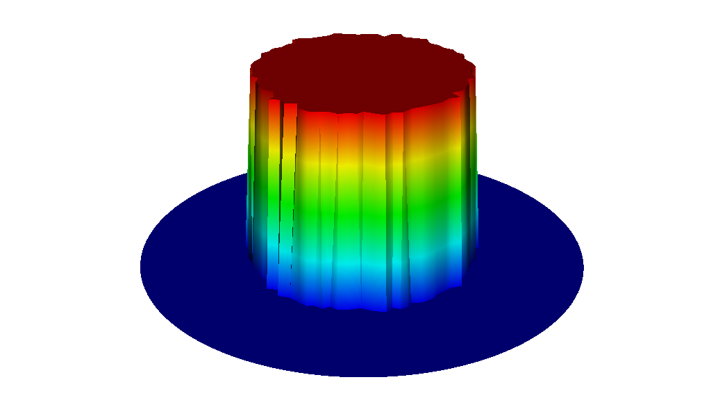
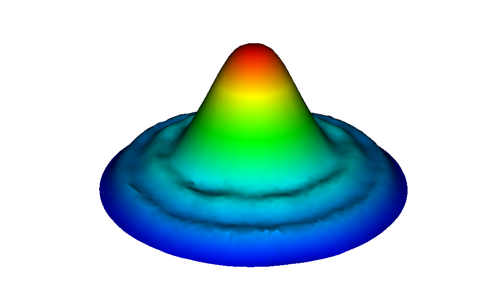
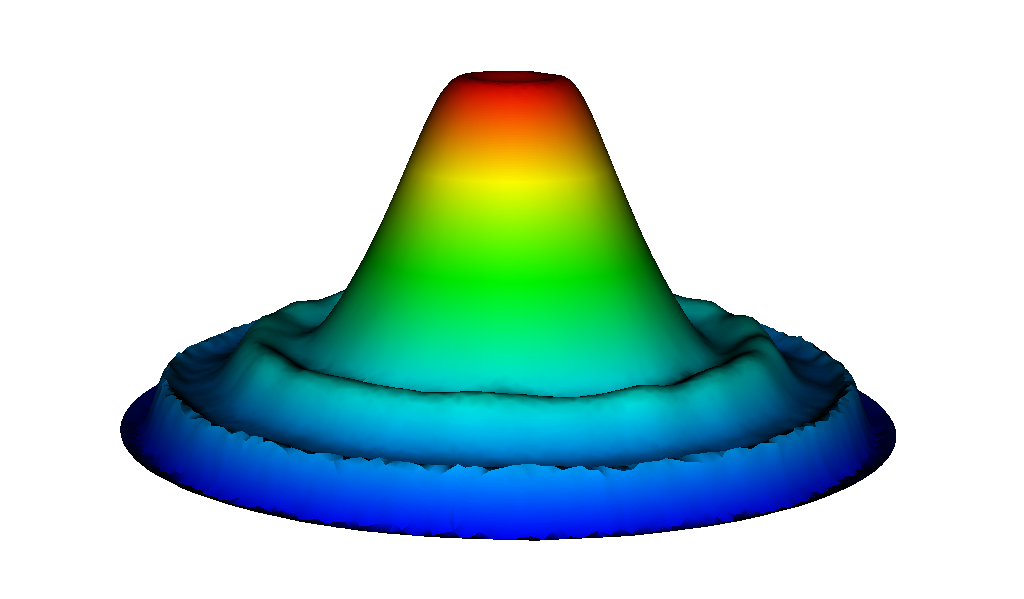
Figure 1: $t=0.25$, DeC(2,2), B1, residual correction, $\varrho$-plot, 3576/13548 elements.

In Figure 2, both correction terms are applied. Without zooming the results are indistinguishable. In the right picture, the bold line is (below) is the numerical solution using the classical correction term (34) and the thin line is the result using the correction (12). This examples demonstrates well the improvement one obtains using entropy correction terms since the not corrected scheme is breaking down.

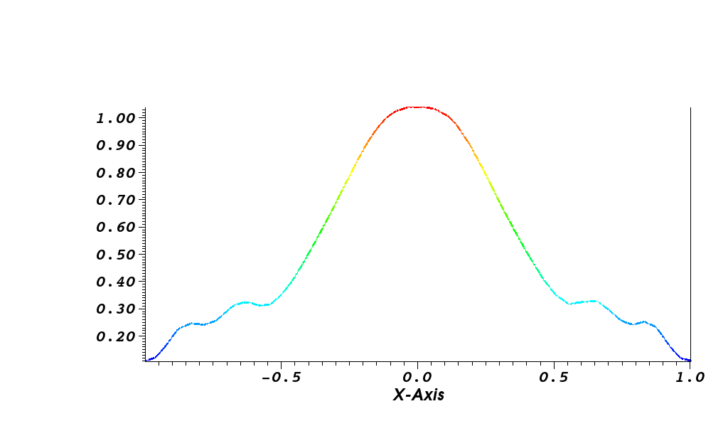
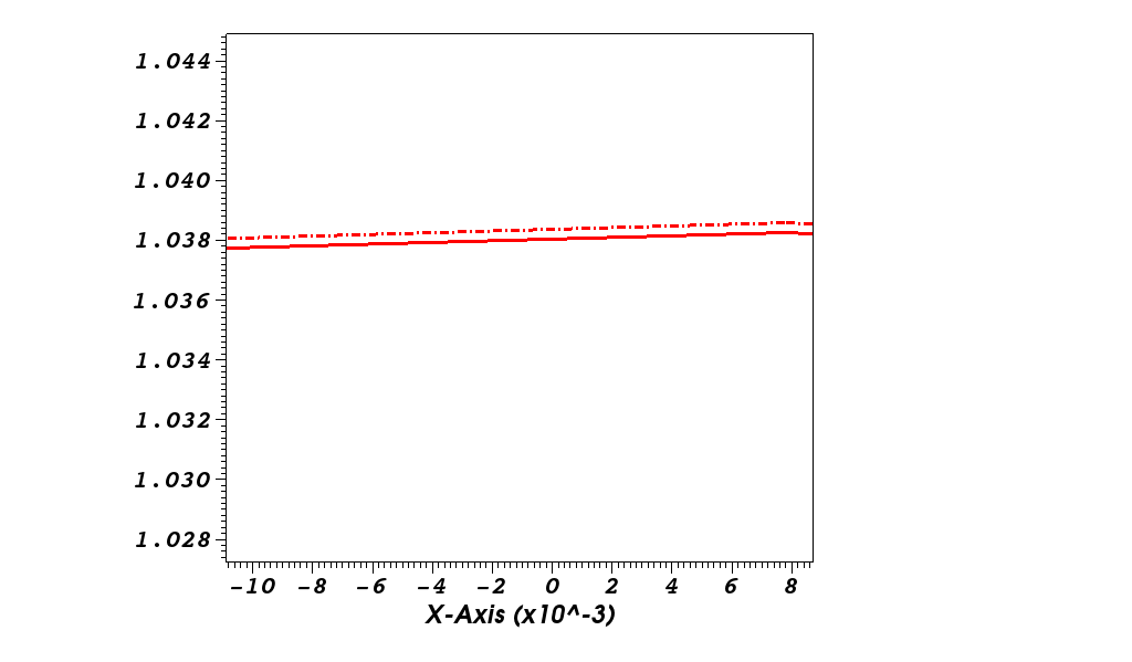
Figure 2: $t=0.25$, DeC(2,2), B1, both correction terms, $\varrho$-plot, 3576 elements.

Up to this point, only SEC/D schemes have been presented. In Figure 3, the same test is considered with wall boundary conditions and the correction term is applied to the fully discrete update step, i.e. the complete bracket in (18) is corrected, resulting in fully discrete EC schemes. As baseline schemes the continuous Galerkin (straight line) and psi schemes (dotted) have been used. One can recognize that the more dissipative character of classical psi scheme has already some positive effect on the behavior of the approximation, although the numerical solutions are EC by construction. This can seen by zooming in since the plateaus are no longer flat using the Galerkin scheme. The reason for this lies in the imposed wall boundary conditions and a further investigation of this behavior will be addressed in future work.

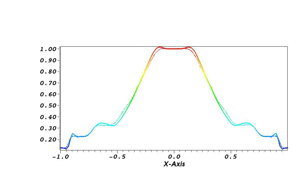
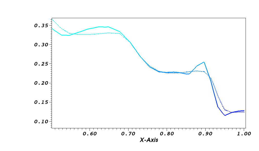
Figure 3: $t=0.25$, DeC(2,2), B1, residual correction, $\varrho$-plot, 8576 elements.

The semidiscrete (dotted) and the fully discrete (solid) Galerkin schemes are compared in Figure 4. Small differences can be recognized, especially around the shocks. However, further investigations and a comparison with the relaxation approach will be part of future work. The correction term (34) is mainly applied. However, analogous results in terms of the quantitative behavior are obtained if the correction term (12) would have been used.

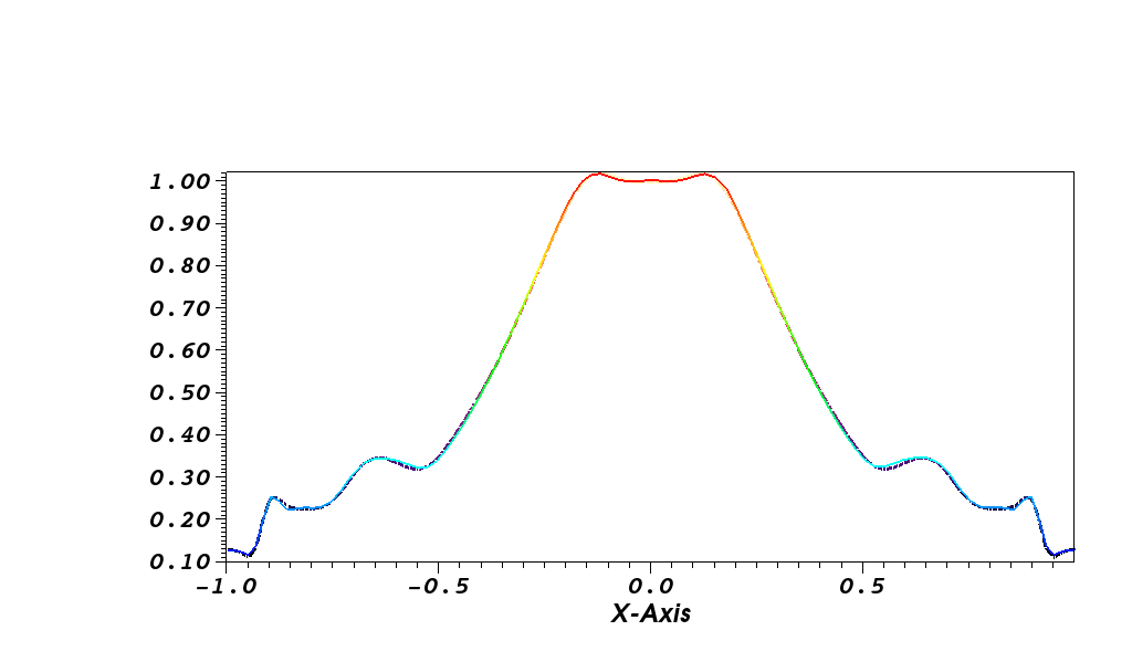
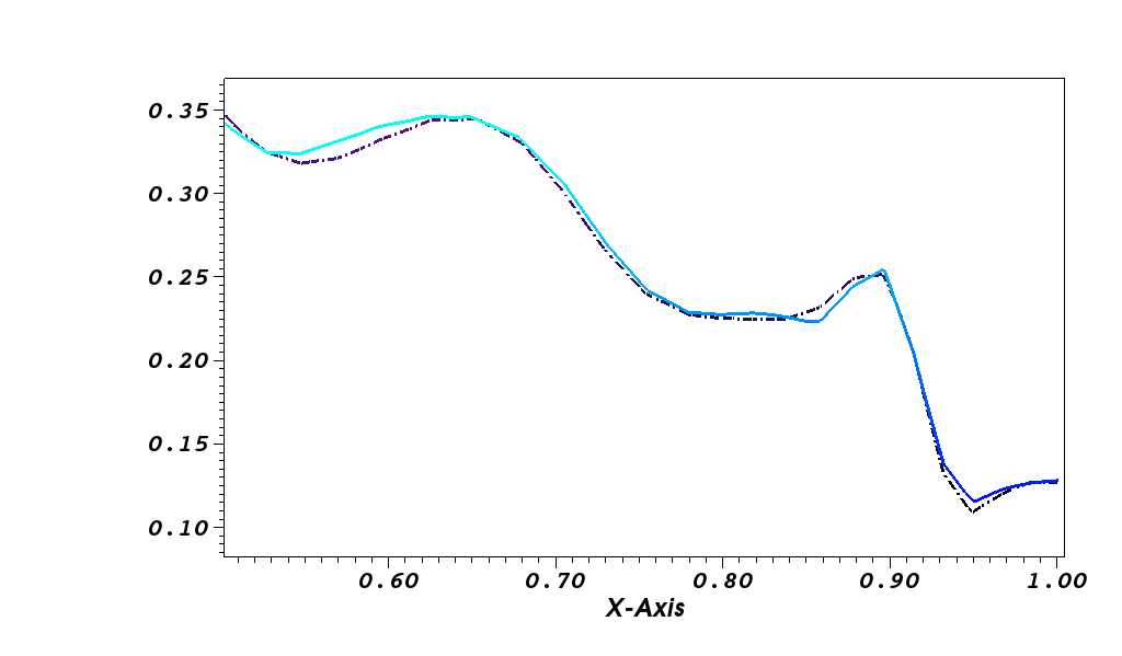
Figure 4: $t=0.25$, DeC(2,2), B1, residual correction, $\varrho$-plot, 8576 elements.

Finally, extensions to higher polynomial degrees are also possible if one can guarantee that both the pressure as well as the density remain positive. This is important for the application of the entropy correction term, not only because of physical reasons but also because of the switch between conservative and entropy variables. In Figure 5, the corrected Galerkin methods are applied and positivity of density and pressure is ensured at all DOFs through the MOOD procedure [12]. However, other limiting strategies can be used as well, e.g. [32].

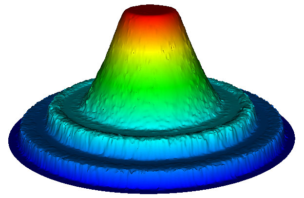
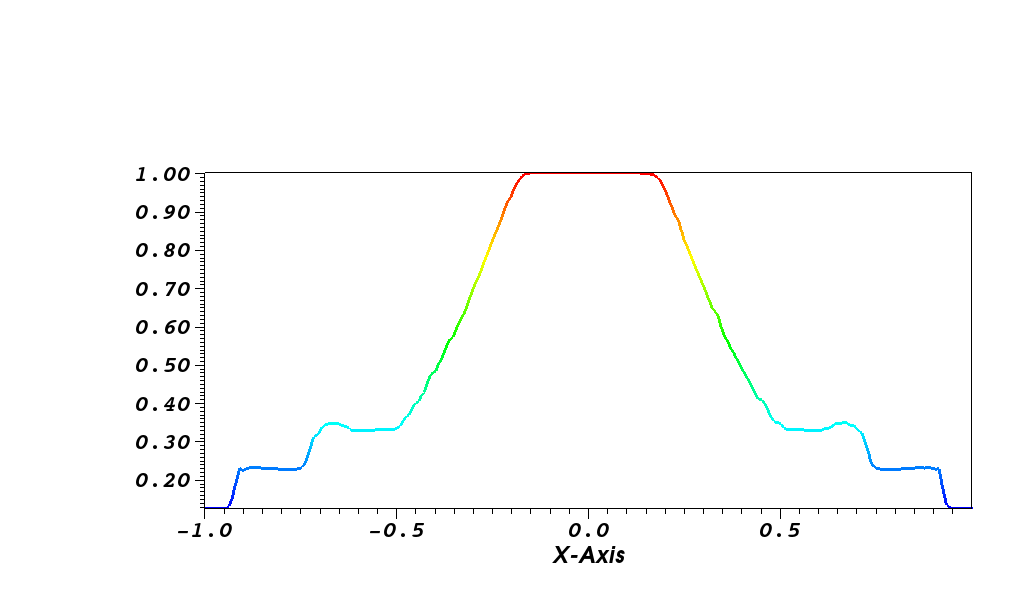
Figure 5: $t=0.25$, DeC(4,4), B3, residual correction, $\varrho$-plot, 13548 elements

A second test is considered for completeness. Here, the classical 1D Shu-Osher test is extended to two dimension with radial speeds and initial conditions

$$(\varrho_{0},v_{x,0},v_{y,0},p_{0})=\begin{cases}(3.857143,\sqrt{2.629\varrho_{0}}\frac{x}{r},\sqrt{2.629\varrho_{0}}\frac{y}{r},10.\overline{3}),\quad&0\leq r\leq 1,\\ (1+0.5\sin(5r),0,0,1),\quad&1<r<4,\\ (1+0.5\sin(20),0,0,1),\quad&4\leq r.\\ \end{cases}$$

Figure 6 shows the initial conditions, an intermediate result after 150 steps, and the final result at $t=1.8$ (373 steps) using the FEC Galerkin method. The SEC Galerkin method is nearly indistinguishable from this result due to the properties of the DeC approach [3, 8] and the usage of high order quadrature rules.

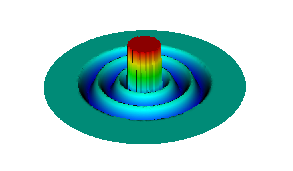
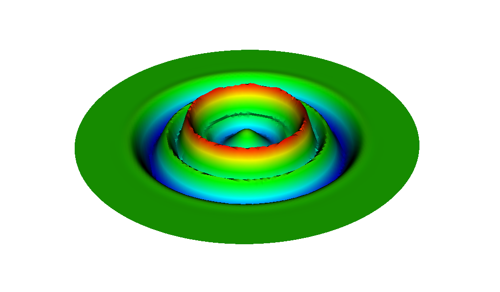
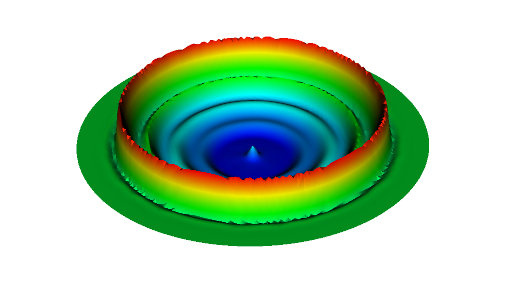
Figure 6: Initial condition, (150 steps) and $t=1.8$ (373 steps), DeC(2,2), B1, classical correction, $\varrho$-plot.

4.2.2 SBP-SAT-DG Setting

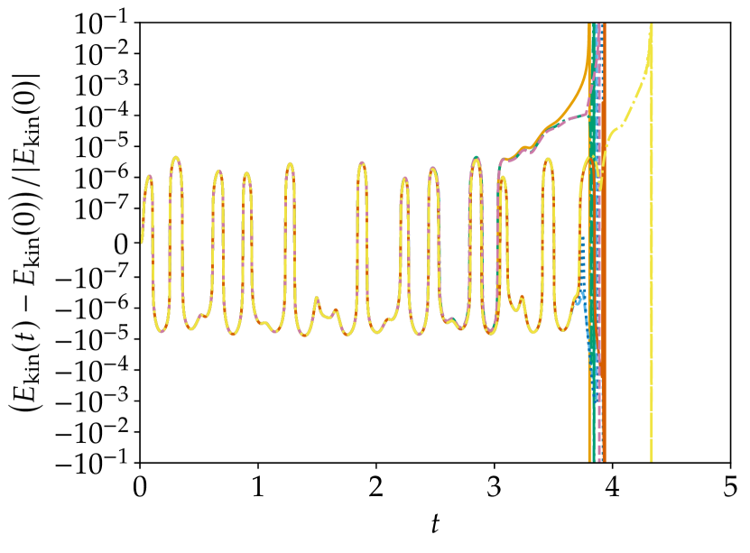
(a) Kinetic Energy.

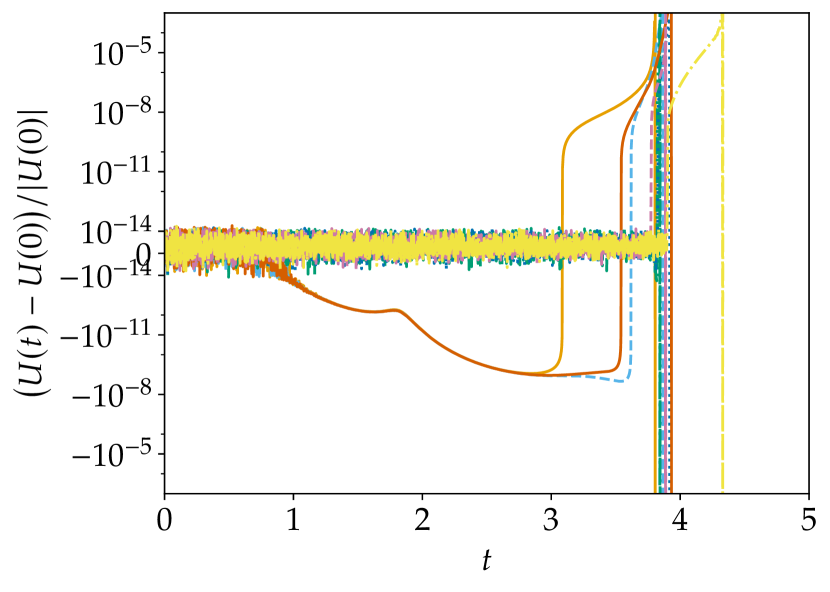
(b) Entropy.

Figure 7: Relative kinetic energy $E_{\mathrm{kin}}$ and entropy $U$ of numerical solutions of the compressible Euler equations with a Taylor-Green

In the second part, a first comparison between the flux differencing approach and the application of correction terms in classical nodal schemes is made. We consider the compressible Euler equations together with Taylor-Green vortex initial conditions given by

$$\varrho(0,x,y) =1, v_{x}(0,x,y) =\sin(x)\cos(y),$$

$$v_{y}(0,x,y) =-\cos(x)\sin(y), p(0,x,y) =\frac{100}{\gamma}+\frac{\cos(2x)+\cos(2y)}{4},$$

for $(x,y)\in[0,2\pi]^{2}$ and periodic boundary conditions. Then, a nodal DG scheme on Lobatto Legendre nodes and the associated Lobatto Legendre quadrature [11, Eq. 25.4.32] for the mass matrix with polynomial degree $p=5$ and $16$ tensor product quadrilateral elements per coordinate direction is used. The numerical flux at the boundaries is the one of [42, Theorem 7.8] and the classical central scheme is used in the interior of each element. The numerical solutions have been integrated in time with the fourth order, ten-stage, SSPRK method of [30] and a constant time step $\Delta t=\frac{\Delta x}{10}\frac{1}{p^{2}+1}$, where $\Delta x$ is the width of one element. Using the central scheme in the interior of each element results in a blow-up at $t\approx 3.8$, cf. Figure 7. Applying a correction for $E_{\mathrm{kin}}$ removes the increase of the kinetic energy before the blow-up and applying a correction for $U$ yields a nearly constant entropy (before the blow-up). As before, there is no big difference between the basic choices of the correction terms (12) and (26). The different weighting does not seem to be crucial for these unstable calculations here. The only minor exception is the correction term for both $E_{\mathrm{kin}}$ and $U$ with the weighting (12). It blows up slightly later at $t\approx 4.3$. The computations using flux differencing schemes in the interior of each element remain stable and do not blow up until $t\approx 35$ is reached, in contrast to the central schemes with correction terms which breaks before. The main purpose of the flux-differencing approach is to split the volume term in the discretization (resulting in a split or skew-symmetric formulation). Other split formulations for the volume term can be found in the literature, cf. [42] and references therein. Another one is based on the flux of Ducros et al. [18], resulting in a DG scheme which is neither entropy stable nor KEP. However, by applying Ducros flux, a splitting for the volume term is obtained and applying to this scheme now the correction terms, one gets the desired results which are presented in Figure 8. Using for instance both the energy and entropy correction, the scheme is similar to the flux differencing scheme using Ranocha’s flux. In particular, the entropy can be conserved and the numerical solutions does not blow up during the computation. Here, we used this numerical flux in the surface term again only for comparison. The numerical flux in the surface integral does not have a major influence on the stability when the correction terms are applied as well. We get indistinguishable results for Ducros’ flux and others in the surface integrals. To clarify, if we apply a proper splitting technique for the volume integral in the DG formulation and use the corrections, we obtain results equivalent to the flux difference approach using these highly sophisticated numerical fluxes. But what is the problem with the classical DG scheme then? Actually, by a closer analysis, it can be recognized that when the DG scheme with entropy corrections results in negative densities and pressures at some nodal values, then neither the change to entropy variables nor the usage of the entropy correction is possible anymore. Thus, the test crashes. The splitting of the volume terms prevents this. An alternative would be the use of positivity preserving limiters or positivity preserving time-integration schemes, which should and will be part of future research. However, the observation made in this subsection can be summarized as follows:

• If the structural properties (SBP) are given, the flux difference approach using the flux of [40, 42, 47] should be applied since it yields an EC/D and KEP scheme with some advantages compared to other fluxes.

• If one prefers other splitting techniques the respective corrections terms will always lead to the desired properties and comparable results to the splitting using Ranocha’s flux. This technique is universally applicable.

• If the structural properties are not given, the correction terms can always be applied and guarantees the desired properties. It will also increase the stability of the scheme.

• If the physical constraints (i.e. positivity of the density and pressure) are ensured, the entropy correction schemes together with a “proper” space discretization are at least as good as state-of-the-art schemes.

It is clear that this is only a first comparison. Further experiments have to be conducted, including for example limiters to avoid the negativity of the density and pressure as done before and seen in Figure 5. Further, also numerical errors and cancellations will be taken more into account. Both are part of future research. Finally, it should be stressed that the correction term is universal whereas the numerical fluxes have to be constructed specifically for each equation. If other problems are considered, one has to work on the construction of numerical fluxes again which have the requested properties. Therefore, more efforts have to been made and it is unknown if this always yields a result. Here, the presented correction term is an enrichment. In Section 5, this topic will be revisited and some examples motivating our formulation formulation will be discussed.

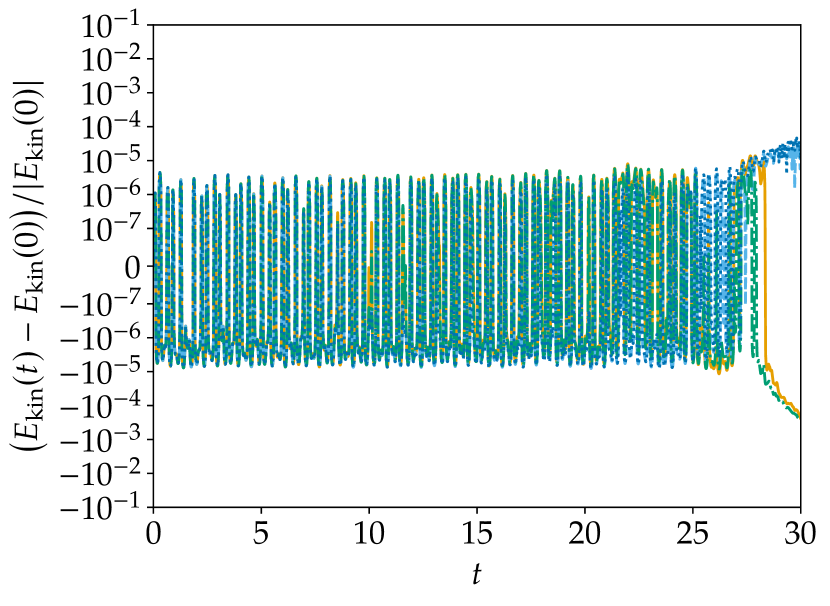
(a) Kinetic Energy.

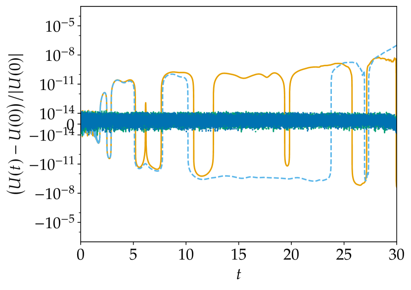
(b) Entropy.

Figure 8: Relative kinetic energy $E_{\mathrm{kin}}$ and entropy $U$ of numerical solutions of the compressible Euler equations with a Taylor-Green vortex initial condition. The nodal discontinuous Galerkin schemes use polynomials of degree $p=5$ on Lobatto Legendre nodes [11, Eq. 25.4.14], the flux difference split form with the flux of Ducros et al. [18, 24] in the interior of each element, and the numerical fluxes of [42, Theorem 7.8] between elements.

4.3 Convergence Test

Here, a convergence test using the initial condition

$$\varrho(0,x,y) =1+\frac{1}{2}\sin(\pi x), v_{x}(0,x,y) =1,$$

$$v_{y}(0,x,y) =0, p(0,x,y) =1,$$

for the Euler equations (38) in the periodic domain $[0,2]\times[0,1]$ using DG schemes is conducted using $(N_{x},N_{y}=1)$ elements in $x$-$y$ direction and polynomials of degree $p=4$. The error of the density at the final time $t=6$ is computed using the Lobatto Legendre quadrature. As can be seen in Table 2, there are no significant differences between the baseline central scheme and the ones applying a correction term, in accordance with results of [1]. For low resolutions, the correction term (34) using a weighting by the mass matrix yields slightly lower errors than the one proposed originally in [1]. Some EOCs are a bit larger than the theoretical EOC of $p+1$. This might be caused by superconvergence effects for DG methods, since the solution returns to the initial condition and the errors are measured at nodal points, at which the solution may observe superconvergence.

Table 2: Convergence rates for central and corrected DG schemes using polynomials of degree $p=4$ for the Euler equations with initial condition (4.3).

	Central Scheme		Correction (34)		Correction (12)
$N_{x}$	$\mathinner{\!\left\lVert\varrho-\varrho_{0}\right\rVert}_{M}$	EOC	$\mathinner{\!\left\lVert\varrho-\varrho_{0}\right\rVert}_{M}$	EOC	$\mathinner{\!\left\lVert\varrho-\varrho_{0}\right\rVert}_{M}$	EOC
5	1.312e-05		1.025e-04		2.537e-04
10	1.394e-06	+3.23	1.994e-06	+5.68	3.041e-06	+6.38
15	3.095e-07	+3.71	3.217e-07	+4.50	3.436e-07	+5.38
20	6.426e-08	+5.46	6.486e-08	+5.57	6.714e-08	+5.68
25	1.810e-08	+5.68	1.819e-08	+5.70	1.836e-08	+5.81

5 Why a New Formulation? Some Motivating Examples

In order to illustrate what we were explaining in the introduction, let us review shortly how entropy preserving schemes are classically obtained. An entropy conservative numerical flux $f^{\mathrm{num}}$ should satisfy Tadmor’s condition:

$$\raisebox{-2.5pt}{\leavevmode\resizebox{0.0pt}{7.5pt}{\raisebox{2.5pt}{$[\mkern-3.0mu[$}}}v\raisebox{-2.5pt}{\leavevmode\resizebox{0.0pt}{7.5pt}{\raisebox{2.5pt}{$]\mkern-3.0mu]$}}}f^{\mathrm{num}}=\raisebox{-2.5pt}{\leavevmode\resizebox{0.0pt}{8.3333pt}{\raisebox{2.5pt}{$[\mkern-3.0mu[$}}}\psi\raisebox{-2.5pt}{\leavevmode\resizebox{0.0pt}{8.3333pt}{\raisebox{2.5pt}{$]\mkern-3.0mu]$}}}$$ (45)

where $v$ is the entropy variable, ( $v=\nabla_{u}S$) and $\psi$ is the potential,

$$g=v^{T}f-\psi$$

where $g$ is the entropy flux.

For systems, $v$ and $f^{\mathrm{num}}$ are vectors, so that (45) must be obtained in a similar way as the Roe average is obtained. This is where complications starts because one need to compute $\psi$ first. In the case of the Euler equations, $S=-\varrho s$ where $s$ is the specific entropy, and since $v=\nabla_{(\varrho,\varrho\mathbf{u},E)}S$, we need an expression of $s$ in term of the conserved variables, or some other set of variables so that the mapping is one-to-one. For inert gases, the specific entropy is defined from Gibb’s relation:

$$T\;ds=d\varepsilon-\frac{p}{\varrho^{2}}d\varrho,$$ (46)

where $T$ is the absolute temperature, $\varepsilon$ the specific heat.

What makes the things relatively easy for the calorically perfect gases case is that specific heat is a constant, as well as $\gamma=\tfrac{c_{p}}{c_{v}}$, so that $\varepsilon=c_{v}T$, and the specific entropy has a simple form

$$s=\log p-\gamma\log\varrho$$

thanks to Mayer’s relation $c_{p}-c_{v}=\tfrac{\mathcal{R}}{M}$, $\mathcal{R}$ being Avogadro’s number and $M$ the molar mass.

For a perfect gas, but a non-calorically perfect one, $\varepsilon=\int_{T_{0}}^{T}c_{v}(T)dT$, and since $p=\varrho\frac{\mathcal{R}}{M}T$, we obtain

$$s=\int_{T_{0}}^{T}\frac{c_{v}(T)}{T}dT-\frac{\mathcal{R}}{M}\log(\varrho)+s_{0},$$

and the situation becomes way more complicated in general, and very dependent on the structure of the function $T\mapsto c_{v}(T)$. It can be analytical (such as in the case of diatomic molecules in air) or tabulated (such as in the NIST-Janaf tables [15]). In the analytical case, it is very likely possible to determine analytically the correct average, such as what has been done for the Roe average and for a complex equation of state, cf. [2] for one example. All of this boils down to identifying the correct variables that make the algebra a bit magic thanks to differentiation rules such as

$$\Delta fg=\underline{f}\Delta g+\overline{g}\Delta f,\quad\Delta h=h_{L}-h_{R},$$

where, for a "well-chosen" parameter $\lambda\in[0,1]$,

$$\overline{f}=\lambda f_{R}+(1-\lambda)f_{L},\qquad\underline{f}=\lambda f_{L}+(1-\lambda)f_{R}.$$

In the case of the Roe average, the magic parameter is $\lambda=\dfrac{\sqrt{\varrho_{L}}}{\sqrt{\varrho_{R}}+\sqrt{\varrho_{L}}}$ and the algebra is much simplified by

$$\underline{\varrho f}=\underline{\varrho}\overline{f},\qquad\underline{f}=\sqrt{\varrho_{L}\varrho_{R}}.$$

Unfortunately, this magic is very much case dependent, and can be very complicated to manage. This why any way of avoiding this tricky algebra for complicated forms of the entropy that a priori needs to have some analytical form is welcomed. Further note that in most cases, this analytical form is not very clean or depends on a look-up table. This is only one example. The situation can become even worse if one asks kinetic energy preservation, and/or additional constraints, such as local preservation of the kinetic momentum.

6 Summary and Conclusions

In this paper, a reinterpretation and extension of entropy correction terms proposed in [1] is given. Based on a characterization of these terms as solutions of certain optimization problems, different correction terms are determined by the choice of discrete norms. Additionally, these terms are adapted to numerical methods such as discontinuous Galerkin schemes. In numerical simulations, the various correction terms are tested both in semidiscrete and fully discrete methods and compared also to flux differencing approaches [21, 24]. These tests demonstrate that there is no significant difference between the two basic choices of correction terms (given in (12) and (33), respectively). All of these optimization problems are solved analytically, resulting in the same runtime performance without the need for an optimization solver.

Using a flux difference formulation shows advantages compared to the application of corrections terms to a simple central scheme. While the correction terms work and preserve the kinetic energy and/or conserve the entropy for the Euler equations as expected, they cannot prevent a blow-up of numerical solutions for a demanding Taylor–Green vortex type initial condition because the corrections terms cannot work correctly due to the generation of negative pressure and densities. If this can be avoided by further techniques, the correction terms can be applied successfully, yielding an entropy conservative scheme that does not blow up during the computation.

This can be interpreted as follows: There is no free lunch. At some point, one has to put work into the methods. The usage and implementation of the entropy correction term is quite simple. However, one has to ensure that physical constraints (positivity of density/pressure in this case) are satisfied to obtain the desired results. On the other hand, the flux difference framework includes some assumptions on the quadrature, i.e. the SBP property as discrete analogue of integration by parts, and the grid structure. Here, a lot of effort has already been invested, as one can recognize by the immense literature in this field. Also the construction of proper two-points fluxes is challenging and it is unclear whether good fluxes can be found for every system as mentioned before. The application of the correction terms does not need these assumptions and is consequently more general. In particular, it can be applied to members of the framework of residual distribution schemes and therefore to nearly any finite-element or finite volume based scheme on any grid. It is a universal tool.

However, it should be stressed out that the success of flux differencing schemes cannot be attributed solely to resulting equations for the kinetic energy or entropy across elements. Inter-element/subcell local equations (which hold for these schemes) might play a role for the improved numerical stability as well. These experiments are only a first comparison and further tests have to be done in this direction but this is not topic of this current paper.

Besides the reinterpretation of the correction terms, their extension to new applications has been conducted. Here, novel generalizations to entropy inequalities, multiple constraints, and kinetic energy preservation for the Euler equations are developed and verified by numerical simulations with a focus on multiple constraints such as conserving the entropy and preserving the kinetic energy simultaneously. Simultaneously, an approach is presented to obtain FEC schemes using only the entropy correction terms.

Appendix A Additional Examples

A.1 Applications to Grid Refinement and Coarsening

There is a certain interest in spatial adaptivity for EC/D semidiscretizations [22]. If space and time adaption has to be performed, grid refinement and coarsening operators transferring the numerical approximation from one grid to another have to be constructed. Ideally, these should respect the entropy dissipative behavior. Consider fine and coarse grids $\Omega_{f}$, $\Omega_{c}$. In the following, it is assumed that a nodal discontinuous element type basis is used and that there are associated coarse/fine and fine/coarse interpolation operators $\operatorname{I}_{f\leftarrow c}$ and $\operatorname{I}_{c\leftarrow f}$. Numerical solutions and operators on the coarse/fine grid will be written using upper indices $c/f$. While standard interpolation and $L^{2}$ projection operators conserve the total mass for reasonable choices of the basis functions and quadrature rule, it is in general impossible to obtain strict inequalities for entropies. Hence, it is of interest to apply an optimization approach similar to the one described in the previous section. However, there are important differences concerning the optimization approach to entropy dissipativity between computations of spatial semidiscretizations and refinement/coarsening operators:

• Computing the time derivative of the entropy results in a linearization of the problem, making it much easier. In fact, a closed solution is given in the previous sections. For the refinement/coarsening operators, such a closed form solution does not seem to be available in general.

• The spatial semidiscretization has to be evaluated for every element and every time step, possibly multiple times. In contrast, the refinement/coarsening operators will be evaluated significantly fewer times.

To sum up, entropy stable refinement/coarsening operators are more expensive but also used less often. Hence, they can be of interest in applications requiring strict entropy inequalities.

Refinement

Given a solution $u^{c}$ on the coarse grid, an optimization problem for the solution $u^{f}$ on the fine grid is

$$\min_{u^{f}}\frac{1}{2}\mathinner{\!\left\lVert u^{f}-\operatorname{I}_{f\leftarrow c}u^{c}\right\rVert}_{M^{f}}^{2}\operatorname{s.t.}\;1^{T}M^{f}u^{f}=1^{T}M^{c}u^{c},\;1^{T}M^{f}U(u^{f})\leq 1^{T}M^{c}U(u^{c}).$$ (47)

Since the norm $\mathinner{\!\left\lVert\cdot\right\rVert}_{M^{f}}$ is strictly convex and coercive and the entropy $U$ is convex, there exists a unique solution of (47). This convex problem can be solved using standard constrained optimization algorithms. For the numerical examples presented below, Ipopt [59] has been used via the interface provided by JuMP [19], using the default options. After some simplifications, the first order necessary condition becomes [35, Theorem 12.1]

$$u^{f}=\operatorname{I}_{f\leftarrow c}u^{c}+\lambda\left(w(u^{f})-\frac{1^{T}M^{f}w(u^{f})}{1^{T}M^{f}1}1\right),$$ (48)

where $\lambda\geq 0$ is a Lagrange multiplier. Assuming that $\operatorname{I}_{f\leftarrow c}u^{c}$ is already a good approximation to $u^{f}$, $w(u^{f})$ can be substituted by $w(\operatorname{I}_{f\leftarrow c}u^{c})$, resulting in

$$\begin{gathered}\min_{\lambda}\frac{1}{2}\lambda^{2}\\ \operatorname{s.t.}\;1^{T}M^{f}U\Biggl{(}\operatorname{I}_{f\leftarrow c}u^{c}+\lambda\left(w(\operatorname{I}_{f\leftarrow c}u^{c})-\frac{1^{T}M^{f}w(\operatorname{I}_{f\leftarrow c}u^{c})}{1^{T}M^{f}1}1\right)\Biggr{)}\leq 1^{T}M^{c}U(u^{c}).\end{gathered}$$ (49)

Compared to (47), where the whole vector $u^{f}$ is the unknown, (49) is a scalar optimization problem which can be solved more efficiently. Indeed, it is basically a scalar root finding procedure: If the interpolation $u^{c}\to\operatorname{I}_{f\leftarrow c}u^{c}$ is entropy dissipative, $\lambda=0$ can be chosen. Otherwise, $\gamma$ has to be chosen with minimal absolute value such that the inequality in (49) is satisfied as an equality.

Coarsening

For a solution $u^{f}$ on the fine grid, an optimization problem for the solution $u^{c}$ on the coarse grid is

$$\min_{u^{c}}\frac{1}{2}\mathinner{\!\left\lVert\operatorname{I}_{f\leftarrow c}u^{c}-u^{f}\right\rVert}_{M^{f}}^{2}\operatorname{s.t.}\;1^{T}M^{c}u^{c}=1^{T}M^{f}u^{f},\;1^{T}M^{c}U(u^{c})\leq 1^{T}M^{f}U(u^{f}).$$ (50)

This is again a convex optimization problem possessing a unique solution.

Numerical Examples

Consider the interval $[-1,1]$ with Lobatto-Legendre nodes for polynomials of degree $\leq 6$ on the fine grid and $\leq 3$ on the coarse grid. The interpolation operators are given by polynomial interpolation and the mass matrices as diagonal matrices using the weights of the corresponding quadrature rule. The exponential entropy $U(u)=\exp(u)$ is used in the following. For the refinement experiment in Figure 9(a), the solution on the coarse grid is obtained by evaluating $\exp(-x^{2})$ on the coarse grid. While the standard interpolation produces spurious entropy, both optimization approaches satisfy the entropy inequality up to the tolerances specified for the algorithms. The optimization results are visually indistinguishable and slightly dissipated compared to the interpolant. The coarsening experiment presented in Figure 9(b) is initialized by evaluating $\exp(x)$ on the fine grid. Both the interpolation and standard $L^{2}$ projection produce spurious amounts of entropy. In contrast, the result obtained by optimization (50) satisfies the desired entropy inequality.

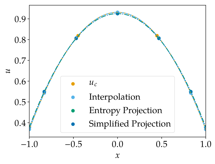
(a) Refinement. The spurious entropy production of the interpolation is $3.566\,10^{-3}$, the approach (47) yields a slight entropy decay of $-3.980\,10^{-8}$ and the simplified problem (49) results in $2.497\,10^{-8}$. Both optimization results deviate from the interpolation by $7.562\,10^{-3}$.

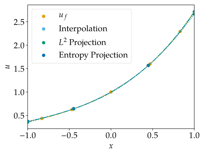
(b) Coarsening. The spurious entropy production of the interpolation is $9.749\,10^{-2}$, the amount of entropy produced by the $L^{2}$ projection is $7.767\,10^{-2}$, and the optimization approach results in a slight entropy decay of $-3.429\,10^{-7}$.

Figure 9: $p$ refinement and coarsening using polynomials of degree $\leq 6$.

A.2 Numerical Simulations - Linear Advection

In the following example, it is demonstrated that an energy/entropy (in-)equality does not imply a good numerical approximation and that the quality of the solution highly depends on the baseline method. One considers the linear advection equation

$$\partial_{t}u(t,x)+\partial_{x}u(t,x) =0, x\in[-1,1],t\in(0,4),$$

$$u(0,x) =u_{0}(x)=\sin(\pi x), x\in[-1,1],$$

with periodic boundary conditions. To solve this problem a nodal DG scheme with $N=16$ uniform elements with polynomial of degree $p=4$ is used where for the calculation of the mass matrix (and then entropy correction term) the closed Newton-Cotes quadrature rule (i.e. $p+1$ equidistant nodes including the boundaries and maximal quadrature accuracy for these nodes, also known as Boole’s rule for $p=4$ [11, Eq. 25.4.14]) is applied. It should be stressed that using equidistant nodes should actually avoided except one follows the approach presented in [25].

The $L^{2}$ entropy/energy $U(u)=\frac{1}{2}u^{2}$ is finally considered and the spatial semidiscretization is integrated in time using SSPRK(10,4) of [30], which is energy stable for linear semidiscretizations [49].

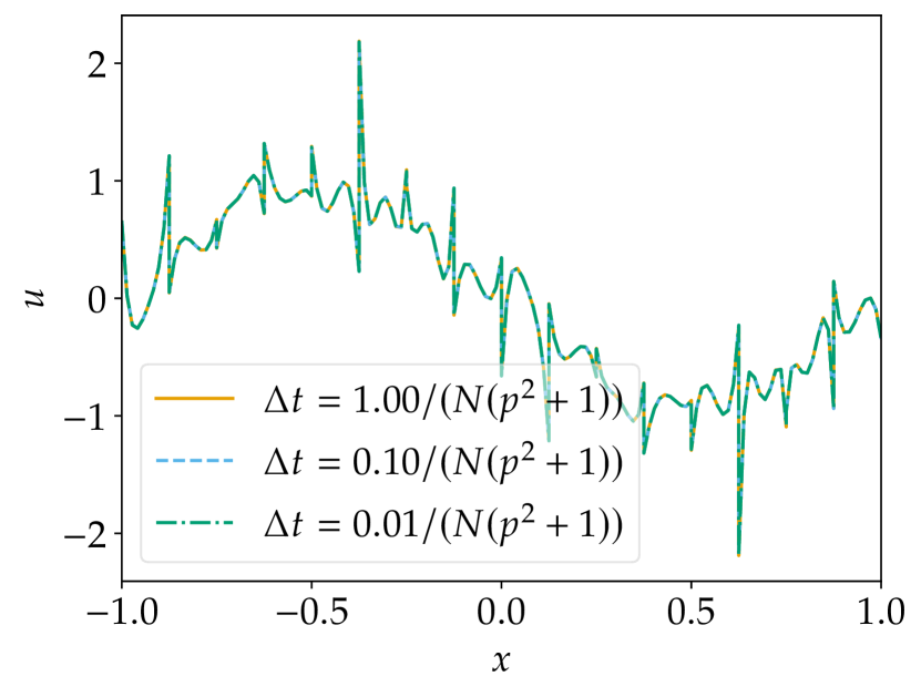
(a) Numerical solutions.

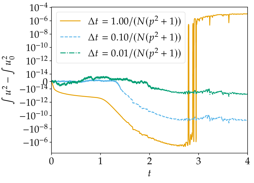
(b) Entropy/energy.

Figure 10: Numerical solutions of the linear advection equation and their energy/entropy, computed using a nodal DG scheme based on closed Newton Cotes quadrature.

Results of these simulations are visualized in Figure 10. Since the semidiscretization is not linear because of the correction terms, the fully discrete scheme does not satisfy an entropy/energy inequality. However, the entropy/energy becomes constant to machine accuracy if the time step $\Delta t$ is refined. Note that the decrease of entropy change corresponds exactly to the order of the time integration method, i.e. decreasing the time step by a factor of ten reduces the entropy change by a factor of $10^{4}$. Nevertheless, the numerical solutions are highly oscillatory. While the entropy correction reduces the amount of oscillations compared to the numerical solution without correction (not shown), the basically bad behavior of the nodal DG schemes with closed Newton Cotes quadrature can still be observed.

A.3 Numerical Simulations - SBP-SAT-FD and Correction terms

We consider the compressible Euler equations together with Taylor-Green vortex initial conditions as in Section 4.2.2. Using classical sixth order SBP central finite difference operators [42] with $100$ nodes per coordinate direction, the numerical solutions have been computed in the time interval $t\in[0,30]$ with the fourth order, ten-stage, strong stability preserving Runge-Kutta method of [30] and a constant time step $\Delta t=\Delta x/8$.

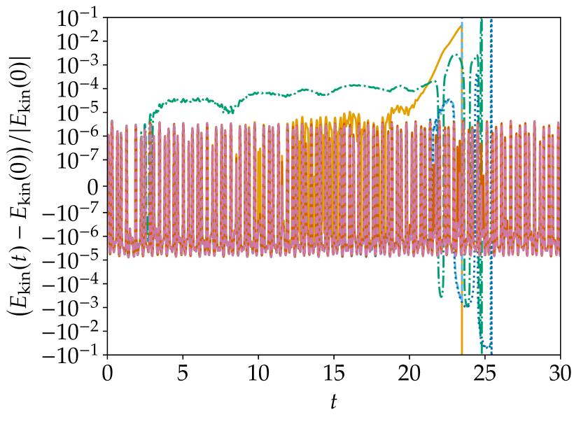
(a) Kinetic Energy.

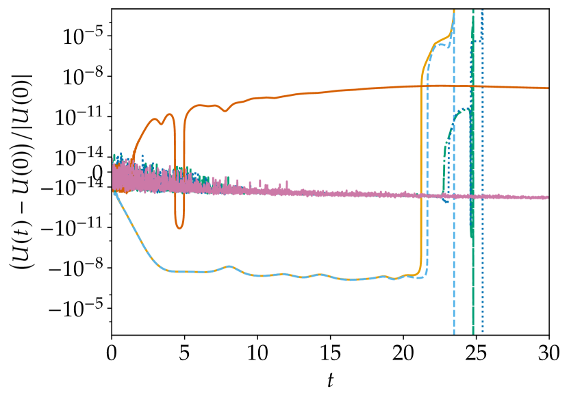
(b) Entropy.

Figure 11: Relative kinetic energy $E_{\mathrm{kin}}$ and entropy $U$ of numerical solutions of the compressible Euler equations with a Taylor-Green vortex initial condition. The finite difference schemes use sixth order classical central stencils and either the classical central scheme with or without correction term or flux difference schemes with numerical fluxes of [39] (see also [24]) or [42, Theorem 7.8].

The relative kinetic energy and entropy of numerical solutions obtained via the classical central scheme with or without corrections or flux difference schemes are visualized in Figure 11. The classical central scheme blows up at $t\approx 23.50$ and strong variations of both the kinetic energy and the entropy can be observed shortly before. Using a correction term for the kinetic energy reduces the variations of $E_{\mathrm{kin}}$ before the blow-up slightly and does not significantly influence the entropy before $t\approx 20$. However, the scheme blows up at approximately the same time.

Using instead a correction term for the entropy, the scheme crashes a bit later at $t\approx 24.82$. This correction term results in an increase of the kinetic energy in this case. The entropy remains constant until it starts to vary before the blow-up. Applying the combined correction term for both entropy and kinetic energy yields to some extent combined results: The oscillations of the kinetic energy are very similar to those with the $E_{\mathrm{kin}}$ correction and the entropy develops similarly to the one using only the $U$ correction. However, the scheme using the combined correction term crashes a bit later ($t\approx 25.46$) than the other ones.

Here, the usage of the correction term can improve the performance of the baseline scheme but can not rescue it. Slightly before the crash, negative pressures and density can be observed. Hence, the correction term cannot be applied and the simulation crashes. The applications of limiters may resolve this problem and will be part of future research in this direction. Nevertheless, substituting the central scheme with a non-trivial flux difference discretization improves the numerical stability significantly if appropriate numerical fluxes are used. In the following, the numerical fluxes of Pirozzoli [39] and Ranocha [42, Theorem 7.8] are used. Both are kinetic energy preserving, i.e. they satisfy (41) analytically. The last flux is also entropy conservative, i.e. the corresponding scheme satisfies (24). The flux difference scheme does not crash during the computation if either one of these fluxes is used. However, it should not be hidden that even using these fluxes the test crashes around $t\approx 35$ but up to this point the flux splitting approach using the flux [42, Theorem 7.8] yield the best results up to our knowledge (without any additional techniques). Both show some oscillations of the kinetic energy with an amplitude similar to the central scheme with $E_{\mathrm{kin}}$ correction. The entropy varies in time if Pirozzoli’s flux is used and the amount of variation is similar to the one for the central scheme before the blow-up. Remarkably, the scheme using the flux of [42, Theorem 7.8] and the central schemes with entropy correction conserve the entropy nearly to machine accuracy. This can not necessarily be expected, since the scheme is only semidiscretely entropy conservative and the time integration scheme can (and will typically) cause variations of $U$. As it can be seen, the flux-splitting with the used fluxes works better than a central scheme with correction. However, it should be pointed out that quite a lot of efforts have been made to construct these types of fluxes and several structural properties have to be assumed to use them. Instead the correction terms are universal tools and do not need these properties. Further, if we apply the correction terms to a skew-symmetric or split formulation of the volume term which does not need necessarily to be energy preserving or entropy conservative then similar results are obtain as for the flux splitting scheme using Ranocha’s flux as seen before.

References

- [1] Rémi Abgrall “A general framework to construct schemes satisfying additional conservation relations. Application to entropy conservative and entropy dissipative schemes” In J. Comput. Phys. 372, 2018, pp. 640–666
- [2] Rémi Abgrall “An extension of Roe’s upwind scheme to algebraic equilibrium real gas models.” In Comput. Fluids 19.2, 1991, pp. 171–182
- [3] Remi Abgrall “High order schemes for hyperbolic problems using globally continuous approximation and avoiding mass matrices” In J. Sci. Comput. 73.2-3 Springer, 2017, pp. 461–494
- [4] Remi Abgrall, Paola Bacigaluppi and Svetlana Tokareva “A high-order nonconservative approach for hyperbolic equations in fluid dynamics” In Comp. Fluids 19.1-3 Elsevier, 2017
- [5] Rémi Abgrall, Paola Bacigaluppi and Svetlana Tokareva “High-order residual distribution scheme for the time-dependent Euler equations of fluid dynamics” In Computers & Mathematics with Applications 78.2 Elsevier, 2019, pp. 274–297
- [6] Remi Abgrall, Adam Larat and Mario Ricchiuto “Construction of very high order residual distribution schemes for steady inviscid flow problems on hybrid unstructured meshes” In J. Comput. Phys. 230.11 Elsevier, 2011, pp. 4103–4136
- [7] Remi Abgrall, Elise le Meledo and Philipp Öffner “On the Connection between Residual Distribution Schemes and Flux Reconstruction” In arXiv preprint arXiv:1807.01261, 2018
- [8] Remi Abgrall, Elise Le Meledo, Philipp Öffner and Davide Torlo “Relaxation Deferred Correction Methods and their Applications to Residual Distribution Schemes” In arXiv preprint arXiv:2106.05005, 2021
- [9] Rémi Abgrall, Jan Nordström, Philipp Öffner and Svetlana Tokareva “Analysis of the SBP-SAT Stabilization for Finite Element Methods Part I: Linear Problems” In Journal of Scientific Computing 85.2 Springer, 2020, pp. 1–29
- [10] Rémi Abgrall, Jan Nordström, Philipp Öffner and Svetlana Tokareva “Analysis of the SBP-SAT stabilization for finite element methods part II: entropy stability” In Communications on Applied Mathematics and Computation Springer, 2021, pp. 1–23
- [11] Milton Abramowitz and Itene A Stegun “Handbook of mathematical functions” National Bureau of Standards, 1972
- [12] Paola Bacigaluppi, Rémi Abgrall and Svetlana Tokareva “" A Posteriori" Limited High Order and Robust Residual Distribution Schemes for Transient Simulations of Fluid Flows in Gas Dynamics” In arXiv preprint arXiv:1902.07773, 2019
- [13] Mark H Carpenter, Matteo Parsani, Travis C Fisher and Eric J Nielsen “Towards an entropy stable spectral element framework for computational fluid dynamics” In 54th AIAA Aerospace Sciences Meeting, 2016 American Institute of AeronauticsAstronautics
- [14] Jesse Chan “On discretely entropy conservative and entropy stable discontinuous Galerkin methods” In J. Comput. Phys. 362 Elsevier, 2018, pp. 346–374
- [15] M.W. Jr. Chase “NIST-JANAF Thermochemical Tables” https://janaf.nist.gov/, Journal of Physical and Chemical Reference Data, 1998
- [16] Tianheng Chen and Chi-Wang Shu “Entropy stable high order discontinuous Galerkin methods with suitable quadrature rules for hyperbolic conservation laws” In J. Comput. Phys. 345 Elsevier, 2017, pp. 427–461
- [17] Tianheng Chen and Chi-Wang Shu “Review of entropy stable discontinuous Galerkin methods for systems of conservation laws on unstructured simplex meshes” In CSIAM Transactions on Applied Mathematics 1.1 Global Science Press, 2020, pp. 1–52 DOI: 10.4208/csiam-am.2020-0003
- [18] F Ducros et al. “High-Order Fluxes for Conservative Skew-Symmetric-Like Schemes in Structured Meshes: Application to Compressible Flows” In J. Comput. Phys. 161.1 Elsevier, 2000, pp. 114–139
- [19] Iain Dunning, Joey Huchette and Miles Lubin “JuMP: A Modeling Language for Mathematical Optimization” In SIAM Review 59.2, 2017, pp. 295–320
- [20] David C Del Rey Fernández, Pieter D Boom and David W Zingg “A generalized framework for nodal first derivative summation-by-parts operators” In J. Comput. Phys. 266 Elsevier, 2014, pp. 214–239
- [21] Travis C Fisher and Mark H Carpenter “High-order entropy stable finite difference schemes for nonlinear conservation laws: Finite domains” In J. Comput. Phys. 252 Elsevier, 2013, pp. 518–557
- [22] Lucas Friedrich et al. “An entropy stable h/p non-conforming discontinuous Galerkin method with the summation-by-parts property” In J. Sci. Comput. 77.2 Springer, 2018, pp. 689–725
- [23] Gregor J Gassner “A Skew-Symmetric Discontinuous Galerkin Spectral Element Discretization and Its Relation to SBP-SAT Finite Difference Methods” In SIAM J. Sci. Comput. 35.3 Society for IndustrialApplied Mathematics, 2013, pp. A1233–A1253
- [24] Gregor J Gassner, Andrew R Winters and David A Kopriva “Split Form Nodal Discontinuous Galerkin Schemes with Summation-By-Parts Property for the Compressible Euler Equations” In J. Comput. Phys. 327 Elsevier, 2016, pp. 39–66
- [25] Jan Glaubitz and Philipp Öffner “Stable discretisations of high-order discontinuous Galerkin methods on equidistant and scattered points” In Applied Numerical Mathematics 151 Elsevier, 2020, pp. 98–118
- [26] Jan Glaubitz, Philipp Öffner, Hendrik Ranocha and Thomas Sonar “Artificial Viscosity for Correction Procedure via Reconstruction Using Summation-by-Parts Operators” In Theory, Numerics and Applications of Hyperbolic Problems II 237, Springer Proceedings in Mathematics & Statistics Cham: Springer International Publishing, 2018, pp. 363–375
- [27] Maria Han Veiga, Philipp Öffner and Davide Torlo “DeC and ADER: Similarities, Differences and an Unified Framework” In Journal of Scientific Computing 87.1 Springer, 2021, pp. 1–35
- [28] Jan S Hesthaven and Tim Warburton “Nodal Discontinuous Galerkin Methods: Algorithms, Analysis, and Applications” 54, Texts in Applied Mathematics New York: Springer Science & Business Media, 2007
- [29] A. Jameson “Formulation of Kinetic Energy Preserving Conservative Schemes for Gas Dynamics and Direct Numerical Simulation of One-Dimensional Viscous Compressible Flow in a Shock Tube Using Entropy and Kinetic Energy Preserving Schemes.” In J Sci Comput 34.2, 2008, pp. 188–208
- [30] David I Ketcheson “Highly Efficient Strong Stability-Preserving Runge-Kutta Methods with Low-Storage Implementations” In SIAM J. Sci. Comput. 30.4 Society for IndustrialApplied Mathematics, 2008, pp. 2113–2136
- [31] David I Ketcheson “Relaxation Runge–Kutta Methods: Conservation and Stability for Inner-Product Norms” In SIAM J. Numer. Anal. 57.6 Society for IndustrialApplied Mathematics, 2019, pp. 2850–2870
- [32] Dmitri Kuzmin “Entropy stabilization and property-preserving limiters for discontinuous Galerkin discretizations of nonlinear hyperbolic equations” In arXiv preprint arXiv:2004.03521, 2020
- [33] Philippe G LeFloch, Jean-Marc Mercier and Christian Rohde “Fully Discrete, Entropy Conservative Schemes of Arbitrary Order” In SIAM Journal on Numerical Analysis 40.5 Society for IndustrialApplied Mathematics, 2002, pp. 1968–1992
- [34] Robert-H Ni “A multiple grid scheme for solving the Euler equations” In 5th Computational Fluid Dynamics Conference, 1981, pp. 1025
- [35] Jorge Nocedal and Stephen J Wright “Numerical Optimization” New York: Springer-Verlag, 1999
- [36] Jan Nordström and Tomas Lundquist “Summation-by-parts in time” In Journal of Computational Physics 251 Elsevier, 2013, pp. 487–499
- [37] Philipp Öffner, Jan Glaubitz and Hendrik Ranocha “Analysis of Artificial Dissipation of Explicit and Implicit Time-Integration Methods” Accepted in International Journal of Numerical Analysis and Modeling, 2019 arXiv:1609.02393 [math.NA]
- [38] Stanley Osher “Riemann solvers, the entropy condition, and difference” In SIAM J. Numer. Anal. 21.2 SIAM, 1984, pp. 217–235
- [39] Sergio Pirozzoli “Numerical Methods for High-Speed Flows” In Annual Review of Fluid Mechanics 43, 2011, pp. 163–194
- [40] Hendrik Ranocha “Comparison of Some Entropy Conservative Numerical Fluxes for the Euler Equations” In J. Sci. Comput. 76.1 Springer, 2018, pp. 216–242 arXiv:1701.02264 [math.NA]
- [41] Hendrik Ranocha “Entropy Conserving and Kinetic Energy Preserving Numerical Methods for the Euler Equations Using Summation-by-Parts Operators” In Spectral and High Order Methods for Partial Differential Equations ICOSAHOM 2018 134, Lecture Notes in Computational Science and Engineering Cham: Springer, 2020, pp. 525–535 DOI: 10.1007/978-3-030-39647-3_42
- [42] Hendrik Ranocha “Generalised Summation-by-Parts Operators and Entropy Stability of Numerical Methods for Hyperbolic Balance Laws”, 2018
- [43] Hendrik Ranocha “On Strong Stability of Explicit Runge–Kutta Methods for Nonlinear Semibounded Operators” In IMA Journal of Numerical Analysis Oxford University Press, 2020 DOI: 10.1093/imanum/drz070
- [44] Hendrik Ranocha “Shallow water equations: Split-form, entropy stable, well-balanced, and positivity preserving numerical methods” In GEM – International Journal on Geomathematics 8.1, 2017, pp. 85–133
- [45] Hendrik Ranocha, Lisandro Dalcin and Matteo Parsani “Fully-Discrete Explicit Locally Entropy-Stable Schemes for the Compressible Euler and Navier-Stokes Equations” In Computers and Mathematics with Applications 80.5 Elsevier, 2020, pp. 1343–1359 DOI: 10.1016/j.camwa.2020.06.016
- [46] Hendrik Ranocha and Gregor J Gassner “Preventing pressure oscillations does not fix local linear stability issues of entropy-based split-form high-order schemes”, 2020 arXiv:2009.13139 [math.NA]
- [47] Hendrik Ranocha and Gregor J Gassner “Preventing pressure oscillations does not fix local linear stability issues of entropy-based split-form high-order schemes” Accepted in Communications on Applied Mathematics and Computation, 2021 arXiv:2009.13139 [math.NA]
- [48] Hendrik Ranocha, Lajos Lóczi and David I Ketcheson “General Relaxation Methods for Initial-Value Problems with Application to Multistep Schemes” In Numerische Mathematik 146 Springer Nature, 2020, pp. 875–906 DOI: 10.1007/s00211-020-01158-4
- [49] Hendrik Ranocha and Philipp Öffner “ Stability of Explicit Runge-Kutta Schemes” In J. Sci. Comput. 75.2, 2018, pp. 1040–1056
- [50] Hendrik Ranocha et al. “Relaxation Runge–Kutta Methods: Fully-Discrete Explicit Entropy-Stable Schemes for the Compressible Euler and Navier–Stokes Equations” In SIAM J. Sci. Comput. 42.2 Society for IndustrialApplied Mathematics, 2020, pp. A612–A638
- [51] Mario Ricchiuto and Remi Abgrall “Explicit Runge–Kutta residual distribution schemes for time dependent problems: second order case” In J. Comput. Phys. 229.16 Elsevier, 2010, pp. 5653–5691
- [52] Philip L Roe “Approximate Riemann solvers, parameter vectors, and difference schemes” In J. Comput. Phys. 43.2 Elsevier, 1981, pp. 357–372
- [53] Vikram Singh and Steven Frankel “Kinetic energy preserving split form flux reconstruction for the compressible Euler equations at Gauss nodes”, Talk presented at the European Workshop on High Order Nonlinear Numerical Methods for Evolutionary PDEs: Theory and Applications (HONOM), 2019
- [54] Björn Sjögreen and Helen C. Yee “High order entropy conservative central schemes for wide ranges of compressible gas dynamics and MHD flows” In J. Comput. Phys. 364 Elsevier, 2018, pp. 153–185
- [55] Zheng Sun and Chi-Wang Shu “Enforcing strong stability of explicit Runge–Kutta methods with superviscosity”, 2019 arXiv:1912.11596 [math.NA]
- [56] Magnus Svärd and Jan Nordström “Review of summation-by-parts schemes for initial-boundary-value problems” In J. Comput. Phys. 268 Elsevier, 2014, pp. 17–38
- [57] Eitan Tadmor “Entropy stability theory for difference approximations of nonlinear conservation laws and related time-dependent problems” In Acta Numerica 12 Cambridge University Press, 2003, pp. 451–512
- [58] Eitan Tadmor “The numerical viscosity of entropy stable schemes for systems of conservation laws. I” In Math. Comp. 49.179 American Mathematical Society, 1987, pp. 91–103
- [59] Andreas Wächter and Lorenz T Biegler “On the implementation of an interior-point filter line-search algorithm for large-scale nonlinear programming” In Mathematical Programming 106.1 Springer, 2006, pp. 25–57