On the Origin of Solar Torsional Oscillations and Extended Solar Cycle

Abstract

We present a nonlinear mean-field model of the solar interior dynamics and dynamo, which reproduces the observed cyclic variations of the global magnetic field of the Sun, as well as the differential rotation and meridional circulation. Using this model, we explain, for the first time, the extended 22-year pattern of the solar torsional oscillations, observed as propagation of zonal variations of the angular velocity from high latitudes to the equator during the time equal to the full dynamo cycle. In the literature, this effect is usually attributed to the so-called “extended solar cycle”. In agreement with the commonly accepted idea our model shows that the torsional oscillations can be driven by a combinations of magnetic field effects acting on turbulent angular momentum transport, and the large-scale Lorentz force. We find that the 22-year pattern of the torsional oscillations can result from a combined effect of an overlap of subsequent magnetic cycles and magnetic quenching of the convective heat transport. The latter effect results in cyclic variations of the meridional circulation in the sunspot formation zone, in agreement with helioseismology results. The variations of the meridional circulation together with other drivers of the torsional oscillations maintain their migration to the equator during the 22-year magnetic cycle, resulting in the observed extended pattern of the torsional oscillations.

1 Introduction

It is widely accepted that differential rotation is one of the most important causes of solar magnetic activity. In the kinematic hydromagnetic dynamo regime, the differential rotation generates large-scale toroidal magnetic field by stretching the poloidal magnetic field component, and the poloidal magnetic field is generated by helical turbulent convection from the toroidal component (Parker, 1955). In the nonlinear dynamical regime, the dynamo-generated magnetic fields can affect the differential rotation as well as turbulent dynamo processes. Thus, observational evidences of the interaction of magnetic field and differential rotation can provide important constraints on theoretical models of the solar dynamo. Since the discovery of zonal variations of the angular velocity (“torsional oscillations”) by Labonte & Howard (1982) it was found that these variations represent a complicated wave-like pattern which consists of alternating zones of accelerated and decelerated plasma flows (Snodgrass & Howard, 1985; Altrock et al., 2008; Howe et al., 2011). Ulrich (2001) found that the wave pattern consists of two oscillatory modes with the periods of 11 and 22 years. Torsional oscillations were linked to ephemeral active regions that emerge at high latitudes during the declining phase of solar cycles, but represent magnetic field of the following cycle (Wilson et al., 1988). In addition, the torsional oscillations were linked to the migrating pattern of coronal green-line emission. These observational results led to the concept of a 22-year long “extended solar cycle”(Altrock, 1997). Using results of the solar magnetic field observations, Stenflo & Guedel (1988) and Stenflo (1992) showed that superposition of different eigenmodes of the global dynamo can result in large-scale magnetic field patterns with extended and overlapping branches in time-latitude diagrams. Similar patterns were reproduced by the mean-field dynamo models, e.g., Brandenburg et al. (1991) or Pipin et al. (2012). Direct numerical simulation are capable to reproduce them as well, e.g., Käpylä et al. (2016). Doppler measurements of the solar rotation by Ulrich (2001) as well as results of helioseismic inversion by Howe et al. (2018) and Kosovichev & Pipin (2019) have demonstrated properties of the “extended” 22-year variations of the zonal flows. In these variations, the zonal flow pattern drifts poleward and equatorward, starting at about 55-degree latitude nearly simultaneously with activity of solar ephemeral active regions of a new solar cycle. The extended mode travels to the equator with the period equal to the full solar magnetic cycle, i.e., about 22 year. The polar-ward branch reaches the polar regions by the time of the solar maximum.

Analysis of helioseismology data for almost two solar cycles by Kosovichev & Pipin (2019) revealed zones of deceleration of the torsional oscillations, which at the surface corresponds to regions of emerging magnetic field (Fig. 1). The torsional oscillation pattern in the near-surface layers obtained by subtracting the mean differential rotation (separately for Solar Cycles 23 and 24), and combining the residuals in the time-latitude diagram is shown in Fig. 1b. For comparison with the evolution of solar magnetic field, in Fig. 2a we present the magnetic butterfly diagram showing the evolution of radial magnetic field. Comparison with the zonal velocity diagram shows that the active regions predominantly emerge at the boundary between the fast and slow zones, at which the fast zone is closer to the equator than the slow zone, as was found in the previous studies. The corresponding zonal acceleration which reflects forcing of the torsional oscillations at the solar surface is shown in Fig. 1c. It clearly reveals the torsional oscillation patterns of both Cycles 23 and 24. By overlaying the zonal acceleration and magnetic field diagrams (Fig. 1d) we find that the active region zones coincide with the flow deceleration zone (blue color). In the polar regions, the deceleration zones correspond to the periods of strong polar magnetic field. This confirms the original ideas that the torsional oscillations are due to the back reaction of solar magnetic fields. Detailed analysis showed that the zonal deceleration originates near the bottom of the convection zone at high latitudes, and migrates to the surface corresponding to magnetic dynamo waves predicted by the Parker’s dynamo theory. On the surface, the torsional oscillation pattern displays two branches migrating poleward and equatorward. The torsional oscillation cycle takes about 22 years. It is important to note that if the torsional oscillation pattern is mainly mediated by the Lorentz force of the near-surface magnetic field, it has to change the sign twice during the full 22-year magnetic cycle. However, in this case, the extended 22-year appearance is not explained. This means that the mechanism of the extended solar cycle phenomenon is related to processes in the deep solar interior. Initially, Malkus & Proctor (1975) showed that the Lorentz force affects efficiency of the dynamo process, and Yoshimura (1981) suggested the first non-kinematic dynamo model that explained the zonal flow variations with the 11-year period. Beside the Lorentz force, other suggested mechanisms of the solar torsional oscillations are related to magnetic perturbation of the Taylor-Proudman balance, and effects of magnetic fields on the heat transport in the solar convection zone (Spruit, 2003; Rempel, 2006). Other mean-field dynamo models (e.g. Kueker et al., 1996; Pipin, 2018) and 3D MHD numerical simulations (e.g. Beaudoin et al., 2013; Guerrero et al., 2016a; Käpylä et al., 2016) also showed that 11-year zonal variations of differential rotation can be caused by the Lorentz force. The simulations produced variations resembling the observed of torsional oscillations, potentially including the extended mode. However, these models did not correctly reproduce the observed cycle duration and time-latitude diagrams of the torsional oscillations, as well as the observed phase relation between the surface magnetic and flow fields (Fig. 1).

In this paper, we present a non-linear mean-field model of the solar dynamo coupled with large-scale dynamics, which explains the extended pattern of the torsional oscillations as well as other properties observed on the solar surface and in the convection zone. The model reproduces well-known properties of the solar dynamo waves that show the 22-year cyclic mode (Stenflo & Guedel, 1988). We extend analysis of the nonlinear dynamo model (Pipin, 2018) that includes effects of the dynamo-generated magnetic field on the angular momentum and heat transport in the solar convection zone. In particular, we discuss the non-dissipative angular momentum flux that is generated by the large-scale magnetic field. In the mean-field hydrodynamics, the non-dissipative angular momentum fluxes (called the $\Lambda$-effect) are parametrized by a tensor (Ruediger, 1989). Theoretically, it was predicted that the large-scale magnetic field produces additional components of the $\Lambda$-effect, which can induce the differential rotation (Kitchatinov et al., 1994; Kueker et al., 1996). This effect was confirmed by numerical simulations of Käpylä (2019).

Our model utilizes the concept of mean-field turbulent dynamo operating in the bulk of the solar convection zone. Some arguments for this type of dynamo were discussed by Brandenburg (2005); Pipin & Kosovichev (2011a) and Kosovichev et al. (2013). In this model, the observed butterfly diagram is explained by migrating dynamo waves, the diffusive migration of which is modified by effects of turbulent pumping and meridional circulation. The effective drift of the large-scale magnetic field because of pumping and meridional circulation was discussed by Pipin (2018). There is still controversy about which type of dynamo operates on the solar convection zone. Therefore, we formulate our model in such a way that, in addition to the dynamo process, it describes the background large-scale hydrodynamic flows, and thus, can be used for the case of the flux-transport dynamo, as well. Among the main conditions for the flux-transport dynamo are the presence of global one-cell meridional circulation and tachocline at the bottom of the convection zone (Dikpati & Charbonneau, 1999; Jouve et al., 2008). The impact of these conditions on the solar/stellar dynamo is a highly debated topic (see, e.g., Zhao et al. 2014; Böning et al. 2017; Rajaguru & Antia 2015; Wright & Drake 2016; Cameron & Schüssler 2017).

The model presented in this paper belongs to the class of distributed dynamos, and, depending on model parameters, can describe both cases with the single- and double-cell meridional circulation. This dynamical mean-field model reproduces the cyclic behavior of the large-scale solar magnetic field, as well as the differential rotation, meridional circulation and their variations with the solar cycle. We analyze effects of various forcing terms (by turning them on and off) on solar-cycle variations of the differential rotation, and show that the observed extended pattern of the solar torsional oscillations results from the overlap of the 22-year dynamo cycles and effects of dynamo-generated magnetic fields on the turbulent angular momentum and heat transport in the solar convection zone.

2 Basic equations.

2.1 The heat transport and angular momentum balance

We employ the standard evolutionary model of the solar thermodynamic structure, which is calculated using the MESA code (Paxton et al., 2011, 2013). The convective turnover time $\tau_{c}$, determined from the MESA code as a function of radius, is assumed to be independent of time. The RMS of convective velocity, $\mathrm{\mathrm{u}_{c}}$, is calculated in the mixing-length approximations from the gradient of mean entropy, $\overline{\mathrm{s}}$,

$$\mathrm{u_{c}=\frac{\ell_{c}}{2}\sqrt{-\frac{g}{2c_{p}}\frac{\partial\overline{s}}{\partial r}},}$$

where $\ell_{c}=\alpha_{MLT}H_{p}$ is the mixing length, $\alpha_{MLT}=1.86$ is the mixing-length theory parameter, and $H_{p}$ is the pressure scale height. The mean-field equation for heat transport is described by the energy conservation law, and takes into account effects of rotation and magnetic field (Pipin & Kitchatinov, 2000):

$$\overline{\rho}\overline{T}\left(\frac{\partial\overline{\mathrm{s}}}{\partial t}+\left(\overline{\mathbf{U}}\cdot\boldsymbol{\nabla}\right)\overline{\mathrm{s}}\right)=-\boldsymbol{\nabla}\cdot\left(\mathbf{F}^{c}+\mathbf{F}^{r}\right)-\hat{T}_{ij}\frac{\partial\overline{U}_{i}}{\partial r_{j}}-\boldsymbol{\boldsymbol{\mathcal{E}}}\cdot\left(\nabla\times\overline{\boldsymbol{B}}\right),$$ (1)

where $\hat{\mathbf{T}}$ is the turbulent stress tensor that includes small-scale fluctuations of velocity and magnetic field:

$$\hat{T}_{\mathrm{ij}}=\overline{u_{i}u_{j}}-\frac{1}{4\pi\overline{\rho}}\left(\overline{b_{i}b_{j}}-\frac{1}{2}\delta_{ij}\overline{\mathbf{b}^{2}}\right),$$ (2)

$\mathbf{u}$ and $\mathbf{b}$ are the turbulent fluctuating velocity and magnetic field, respectively. Other quantities in Eq.(1) include the mean electromotive force, $\boldsymbol{\mathcal{E}}=\left\langle\mathbf{u\times b}\right\rangle$, $\overline{\rho}$ is the mean density, $\overline{T}$ - the mean temperature, $\mathbf{F}^{c}$ - the eddy convective flux, and $\mathbf{F}^{r}$ is the radiative flux. For calculation of $\hat{\mathbf{T}}$, $\boldsymbol{\boldsymbol{\mathcal{E}}}$ and $\mathbf{F}^{c}$, we employ analytical results that were obtained earlier using the mean-field magnetohydrodynamics framework. These results take into account effects of the global rotation and magnetic field on turbulence. Some important details and references are given below and in Appendix.

The magnitude of $\hat{\mathbf{T}}$, $\boldsymbol{\boldsymbol{\mathcal{E}}}$ and $\mathbf{F}^{c}$ in Eq.(1) depends on the RMS of convective velocity, $\mathrm{\mathrm{u}_{c}}$, efficiency of the Coriolis force, and the strength of large-scale magnetic field. The effect of the Coriolis force is determined by parameter $\Omega^{*}=2\Omega_{0}\tau_{c}$, where $\tau_{c}$ is the convective turnover time. We assume that the characteristic solar rotation rate corresponds to the rotation rate of the tachocline at 30^∘ latitude, i.e., $\Omega_{0}/2\pi=430$nHz (Kosovichev et al., 1997). The influence of large-scale magnetic field on convective turbulence is determined by parameter $\mathrm{\beta=\left|\overline{\mathbf{B}}\right|/\sqrt{4\pi\overline{\rho}u_{c}{}^{2}}}$.

For the anisotropic convective flux, we employ the expression suggested by Kitchatinov et al. (1994):

$$\mathrm{F_{i}^{c}=-\overline{\rho}\overline{T}\chi_{ij}\nabla_{j}\overline{s}.}$$ (3)

Further details about dependence of the eddy thermal conductivity tensor, $\mathrm{\chi_{ij}}$, on the global rotation and large-scale magnetic field are given in Appendix A, in Eq.(A13).

For the angular momentum balance, we use the model recently developed by Pipin (2018). The model describes evolution of the mean axisymmetric velocity: $\mathrm{\mathbf{\overline{U}}=\mathbf{\overline{U}}^{m}+r\sin\theta\Omega\hat{\mathbf{\boldsymbol{\phi}}}}$, where $\boldsymbol{\hat{\phi}}$ is the azimuthal unit vector, and $\mathbf{\overline{U}}^{m}$ is the meridional circulation velocity. We employ the anelastic approximation. Conservation of the angular momentum determines distribution of the angular velocity inside the convection zone:

$$\frac{\partial}{\partial t}\overline{\rho}r^{2}\sin^{2}\theta\Omega = -\boldsymbol{\nabla\cdot}\left(r\sin\theta\overline{\rho}\left(\hat{\mathbf{T}}_{\phi}+r\sin\theta\Omega\mathbf{\overline{U}^{m}}\right)\right)$$

$$+ \boldsymbol{\nabla\cdot}\left(r\sin\theta\frac{\overline{\mathbf{B}}\overline{B}_{\phi}}{4\pi}\right).$$

The meridional circulation is determined from equation for the azimuthal component of large-scale vorticity, $\mathrm{\overline{\omega}=\left(\boldsymbol{\nabla}\times\overline{\mathbf{U}}^{m}\right)_{\phi}}$:

$$\mathrm{\frac{\partial\omega}{\partial t}\!\!\!} \mathrm{\!\!=\!\!\!\!} \mathrm{r\sin\theta\boldsymbol{\nabla}\cdot\left(\frac{\hat{\boldsymbol{\phi}}\times\boldsymbol{\nabla\cdot}\overline{\rho}\hat{\mathbf{T}}}{r\overline{\rho}\sin\theta}-\frac{\mathbf{\overline{U}}^{m}\overline{\omega}}{r\sin\theta}\right)}$$

$$+ \mathrm{r}\sin\theta\frac{\partial\Omega^{2}}{\partial z}-\mathrm{\frac{g}{c_{p}r}\frac{\partial\overline{s}}{\partial\theta}}+F_{L}^{(p)}$$

where $\mathrm{\partial/\partial z=\cos\theta\partial/\partial r-\sin\theta/r\cdot\partial/\partial\theta}$ is the gradient along the axis of rotation. The first line in Eq.(2.1) describes dissipation and advection of the large-scale vorticity and meridional circulation; the second line describes effects of the centrifugal force, the thermal wind, and the poloidal component of the large-scale Lorentz force, $F_{L}^{(p)}$ (see, the Eq(2.2)).

Both, the eddy thermal conductivity, $\chi_{T}$, and viscosity $\nu_{T}$, are determined from the mixing-length theory:

$$\chi_{T} = \frac{\ell^{2}}{6}\sqrt{-\frac{g}{2c_{p}}\frac{\partial\overline{s}}{\partial r}},$$

$$\nu_{T} = \mathrm{Pr}_{T}\chi_{T},$$

where $\mathrm{Pr}_{T}$ is the turbulent Prandtl number. It is assumed that $\mathrm{Pr}_{T}=3/4$.

The described model of the mean-field heat transport and angular momentum balance follow the line of work of Kitchatinov et al. (1994). In terms of the original theory of the $\Lambda$-effect, the model reproduces results of Kitchatinov & Olemskoy (2011). In this case, the mean-field model reproduces the solar-like differential rotation profile with one meridional circulation cell per hemisphere. The double-cell meridional circulation structure is reproduced when inversion of the $\Lambda$-effect radial profile in the solar convection zone is taken into account (Bekki & Yokoyama, 2017). Such inversion can result from radial inhomogeneity of the convective turnover time, $\tau_{c}$ (Pipin & Kosovichev, 2018). In our model, it is calculated using the mixing-length approximation, $\tau_{c}=\ell_{c}/\mathrm{u_{c}}$. According to the convection zone properties given by the MESA code, $\tau_{c}$ increases sharply towards the bottom of convection zone. This results in a secondary meridional circulation cell (Pipin & Kosovichev, 2018). The helioseismology results are still contradictory about the strength and parameters of the meridional circulation near the bottom of the convection zone (see, e.g., Zhao et al. 2014; Böning et al. 2017; Rajaguru & Antia 2015; Wright & Drake 2016; Cameron & Schüssler 2017). Therefore, we consider both cases of the single- and double-cell meridional circulation structure. The smooth transition between these two cases can be controlled by variations of the mixing-length parameter, $\ell_{c}$, using the following ansatz of Kitchatinov & Nepomnyashchikh (2017):

$$\ell_{c}=\ell_{\mathrm{min}}+\frac{1}{2}\left(\ell_{c}^{(0)}-\ell_{\mathrm{min}}\right)\left[1+\mathrm{erf}\left(\frac{r-(r_{b}+\ell_{\mathrm{min}})}{R_{\odot}d}\right)\right],$$ (6)

where $\ell_{c}^{(0)}$ is the mixing-length parameter from the MESA code, $r_{b}=0.728R_{\odot}$ is the radius of the bottom of the convection zone, $d=0.02$. We use $\ell_{\mathrm{min}}$ as a control parameter to model saturation of $\tau_{c}$ variations in the $\Lambda$-tensor. For $\ell_{\mathrm{min}}\leq 0.01R_{\odot}$, we obtain solutions with the double cell meridional circulation structure. In another development of the models of Pipin & Kosovichev (2018) and Pipin (2018), we add the tachocline. Similarly to Rempel (2006), we use a phenomenological approach to model the angular velocity profile in the tachocline. Within the tachocline layer, we solve Eq.(2.1) assuming continuity of the stress and angular velocity at the bottom of the convection zone and the solid body rotation state of the radiative zone at inner boundary, $r_{t}=0.68R_{\odot}$.

The turbulent parameters below the convection zone are defined following the results of Ludwig et al. (1999), also see Paxton et al. (2011). We apply an exponential decrease of all turbulent coefficients (except the eddy viscosity and eddy diffusivity) with decrement -100, i.e., they are multiplied by a factor of $\exp\left(-100z/R\right)$, where $z$ is the distance from the bottom of the convection zone. We keep the eddy viscosity and eddy diffusivity finite at the bottom of the tachocline, i.e., for the eddy viscosity coefficient profile within the tachocline we put

$$\nu_{T}^{(t)}=\frac{\nu_{T}^{(c)}}{\left(\nu_{T}^{(0)}+\nu_{T}^{(c)}\right)}\left(\nu_{T}^{(0)}+\nu_{T}^{(c)}\exp\left(-100z\right)\right),$$ (7)

where $\nu_{T}^{(c)}$ is the value at the bottom of the convection zone, $\nu_{T}^{(0)}$ is the value inside the tachocline, $z$ is the distance from the bottom of the convection zone. We use $\nu_{T}^{(c)}/\nu_{T}^{(0)}=20$ in the model. The same parametrization is used for the eddy diffusivity. Figure 2 shows the global hydrodynamic models M1 and M2 (Table 1) with one and two circulation cells along the radius in the solar convection zone. Our models show good agreement with the results of helioseismology in terms of the differential rotation profile. The maximum difference is less than 10 nHz. Although, the magnitude of the radial shear in tachocline is about twice higher than in the observations, and in the subsurface shear layer, it is about twice smaller.

2.2 Dynamo model

Evolution of the large-scale axisymmetric magnetic field, $\overline{\mathbf{B}}$, is governed the mean-field induction equation (Krause & Rädler, 1980),

$$\mathrm{\partial_{t}\overline{\mathbf{B}}=\boldsymbol{\nabla}\times\left(\boldsymbol{\mathcal{E}}+\mathbf{\overline{U}}\times\overline{\mathbf{B}}\right)},$$ (8)

where $\boldsymbol{\mathcal{E}}=\left\langle\mathbf{u\times b}\right\rangle$ is the mean electromotive force with $\mathbf{u}$ and $\mathbf{b}$ standing for fluctuating turbulent velocity and magnetic field respectively. We employ the mean electromotive force in the form:

$$\mathcal{E}_{i}=\left(\alpha_{ij}+\gamma_{ij}\right)\overline{B}_{j}-\eta_{ijk}\nabla_{j}\overline{B}_{k}.$$ (9)

where symmetric tensor $\alpha_{ij}$ models generation of the large-scale magnetic field by the $\alpha$-effect; antisymmetric tensor $\gamma_{ij}$ controls the mean drift of the large-scale magnetic fields in turbulent medium; the tensor $\eta_{ijk}$ governs the anisotropic turbulent diffusion. The reader can find further details about the dynamo model in Pipin (2018).

The anisotropic diffusion plays a particular role in our model because it affects overlap of the magnetic cycles, and the extended mode of the dynamo waves (Pipin & Kosovichev, 2014). We employ the anisotropic diffusion tensor following the formulation of Pipin (2008) and Pipin & Kosovichev (2014):

$$\eta_{ijk} = 3\eta_{T}\left\{\left(2f_{1}^{(a)}-f_{2}^{(d)}\right)\varepsilon_{ijk}+2f_{1}^{(a)}\frac{\Omega_{i}\Omega_{n}}{\Omega^{2}}\varepsilon_{jnk}\right\}$$

$$+ \eta_{A}\phi_{1}\left(g_{n}g_{j}\varepsilon_{ink}-\varepsilon_{ijk}\right)$$

where $\mathbf{g}$ is the radial unit vector, $\eta_{T}$ is the magnetic diffusion coefficient, $\eta_{A}=a\eta_{T}$, and $a$ is a parameter of the turbulence anisotropy. The quenching functions $f_{1,2}^{(a,d)}$ and $\phi_{1}$ are formulated by Pipin & Kosovichev (2014).

The $\alpha$-effect takes into account kinetic and magnetic helicities in the following form:

$$\mathrm{\alpha_{ij}} \mathrm{=} \mathrm{C_{\alpha}\frac{\nu_{T}}{Pm_{T}}\psi_{\alpha}(\beta)\alpha_{ij}^{(H)}+\alpha_{ij}^{(M)}\frac{\overline{\chi}\tau_{c}}{4\pi\overline{\rho}\ell^{2}}}$$ (11)

where $\mathrm{C_{\alpha}}$ is a free parameter which controls the strength of the $\alpha$-effect due to turbulent kinetic helicity; tensors $\mathrm{\alpha_{ij}^{(H)}}$ and $\mathrm{\alpha_{ij}^{(M)}}$ express the kinetic and magnetic helicity parts of the $\alpha$-effect, respectively; $\mathrm{Pm_{T}}=\nu_{T}/\mathrm{\eta_{T}}$ is the turbulent magnetic Prandtl number, and $\overline{\chi}=\left\langle\mathbf{a}\cdot\mathbf{b}\right\rangle$ ($\mathbf{a}$ and $\mathbf{b}$ are fluctuating parts of the magnetic field vector-potential and magnetic field vector). Both, $\mathrm{\alpha_{ij}^{(H)}}$ and $\mathrm{\alpha_{ij}^{(M)}}$, depend on the Coriolis number. Function $\psi_{\alpha}(\beta)$ controls the so-called “algebraic” quenching of the $\alpha$-effect, where $\mathrm{\beta=\left|\overline{\mathbf{B}}\right|/\sqrt{4\pi\overline{\rho}u_{c}^{2}}}$, $\mathrm{u_{c}}$ is the RMS of the convective velocity. It is found that $\psi_{\alpha}(\beta)\sim\beta^{-3}$ for $\beta\gg 1$. The $\alpha$-effect tensors, $\mathrm{\alpha_{ij}^{(H)}}$ and $\mathrm{\alpha_{ij}^{(M)}}$, are given by Pipin (2018). Evolution of the small-scale magnetic helicity, $\overline{\chi}=\left\langle\mathbf{a}\cdot\mathbf{b}\right\rangle$, is governed by the magnetic helicity conservation law (Pipin & Kosovichev, 2011b).

We assume that the large-scale magnetic field is vanished: $B=0,\,A=0$; and that the normal component of the magnetic field and the tangential components of the mean electromotive force are continuous at the interface between the tachocline and the convection zone. Following ideas of Moss & Brandenburg (1992) and Pipin & Kosovichev (2011a), we formulate the top boundary condition in the form that allows penetration of the toroidal magnetic field to the surface:

$$\delta\frac{\eta_{T}}{r_{e}}B\left(1+\left(\frac{\left|B\right|}{B_{\mathrm{esq}}}\right)^{2}\right)+\left(1-\delta\right)\mathcal{E}_{\theta} = 0,$$ (12)

where $r_{e}=0.99R_{\odot}$, and parameter $\delta=0.99$ and $B_{\mathrm{esq}}=50$G. The magnetic field potential outside the domain is

$$A^{(vac)}\left(r,\mu\right)=\sum a_{n}\left(\frac{r_{e}}{r}\right)^{n}\sqrt{1-\mu^{2}}P_{n}^{1}\left(\mu\right).$$ (13)

The influence of magnetic field and meridional circulation on the angular velocity profiles can be characterized by the local forces caused by magnetic feedback on the turbulent stresses, $\hat{\mathbf{T}}$. We introduce the following notations for components of the force per unit mass:

$$F_{I} = -\frac{1}{\overline{\rho}r\sin\theta}\boldsymbol{\nabla\cdot}\left(r\sin\theta\overline{\rho}\hat{\mathbf{T}}_{\phi}\left(\boldsymbol{B}=0\right)\right)$$ (14)

$$F_{\ell} = -\frac{1}{\overline{\rho}r\sin\theta}\boldsymbol{\nabla\cdot}\left(r\sin\theta\overline{\rho}\left\{\hat{\mathbf{T}}_{\phi}-\hat{\mathbf{T}}_{\phi}\left(\boldsymbol{B}=0\right)\right\}\right),$$ (15)

$$F_{L}^{(t)} = \frac{1}{\overline{\rho}r\sin\theta}\boldsymbol{\nabla\cdot}\left(r\sin\theta\frac{\overline{\mathbf{B}}\overline{B}_{\phi}}{4\pi}\right),$$ (16)

$$F_{L}^{(p)} = \frac{1}{4\pi\overline{\rho}}\left(\overline{\mathbf{B}}\boldsymbol{\cdot\nabla}\right)\left(\boldsymbol{\nabla}\times\overline{\mathbf{B}}\right)_{\phi}-\frac{1}{4\pi\overline{\rho}}\left(\left(\boldsymbol{\nabla}\times\overline{\mathbf{B}}\right)\boldsymbol{\cdot\nabla}\right)\overline{\mathbf{B}}{}_{\phi}$$

$$+ \mathrm{\frac{1}{\overline{\rho}^{2}}\left[\!\!\boldsymbol{\nabla}\overline{\rho}\times\left(\!\!\boldsymbol{\nabla}\frac{\overline{\mathbf{B}}^{2}}{8\pi}-\frac{\left(\overline{\mathbf{B}}\boldsymbol{\cdot\nabla}\right)\overline{\mathbf{B}}}{4\pi}\!\right)\!\!\right]_{\phi}}$$

$$F_{U} = -\frac{1}{\overline{\rho}r\sin\theta}\boldsymbol{\nabla\cdot}\left(r^{2}\sin^{2}\theta\overline{\rho}\Omega\mathbf{\overline{U}^{m}}\right),$$ (18)

$$F_{H} = -\frac{1}{\overline{\rho}r\sin\theta}\boldsymbol{\nabla\cdot}\left(r\sin\theta\overline{\rho}\hat{\mathbf{T}}_{\phi}^{\left(\Lambda\right)}{\left(H^{(0)}\right)}\right),$$ (19)

Here, $F_{I}$ represents the hydrodynamic inertial force of the solar differential rotation. Contribution $F_{\ell}$ is caused by the Maxwell stresses of the small-scale magnetic fields. This effect was computed analytically in the previous studies cited above. It is zero in absence of magnetic field. $F_{L}^{(t,p)}$ stands for the of the large-scale magnetic field, and $F_{U}$ is the azimuthal force due to the effect of the meridional circulation. Contribution $F_{H}$ describes the dynamo-induced latitudinal angular momentum flux by the $\Lambda$-effect. In the dynamo theory, see, e.g. Kueker et al. (1996), the magnetically induced $\Lambda$ effect is usually denoted by $H^{(0)}$ (see details in Appendix). The $H^{(0)}$ term results from the small-scale Maxwell stresses $\overline{b_{\theta}b_{\phi}}/4\pi\overline{\rho}$, which stem from perturbations of the large-scale magnetic field by turbulence. This effect was calculated analytically in the above cited papers. It was found that $H^{(0)}$ can be represented as the sum of two contributions,

$$H^{(0)}=H^{(0,a)}+H^{(0,\rho)},$$ (20)

where $H^{(0,a)}$ originates from anisotropy of convective turbulence (Kichatinov, 1988), and $H^{(0,\rho)}$ results from the density stratification (Kueker et al., 1996; Pipin, 1999). The signs of $H^{(0,a)}$ and $H^{(0,\rho)}$ are opposite. Unlike the other contributions of the $\Lambda$-effect, $H^{(0)}$ grows with the increase of energy of the large-scale magnetic field when the field is weak, $\beta<1$. Further theoretical details are given in Appendix A. Another promising source of the dynamo induced $\Lambda$ effect stems from the convective heat flux (Rogachevskii & Kleeorin, 2018). We postpone discussion of this effect for future papers.

The dynamo cycle results in variations of large-scale torque forces. Below we discuss properties of the stationary phase of the numerical solution. We consider deviations of the force components from their mean values (time averages). In addition, there is an effect of variations of the entropy gradient because the magnetic field affects the heat transport by means of magnetic quenching of the turbulent eddy heat conductivity, as well as the energy sinks and gains associated with magnetic field generation and dissipation (see Eq. 1). Consequently, the entropy variations result in perturbations of the Taylor-Proudman balance (Durney, 1999) and variations of the meridional circulation. The latter affects the magnitude and distribution of the differential rotation in the solar convection zone, and play important role in the mechanism of torsional oscillations.

3 Results

Results of our numerical experiments show that there are two necessary conditions for appearance of the extended 22-year pattern of the torsional oscillations. The first one is existence of the 22-year mode in the dynamo wave pattern and the subsequent overlap of magnetic cycles on the solar surface. The second one is magnetic quenching of the eddy thermal conductivity. This effect results in the cyclic modulation of the thermal wind associated with the mean entropy gradient, and, correspondingly, the Taylor-Proudman balance and the meridional circulation. The latter affects the torsional oscillations by means the forces $F_{U}$ and $F_{I}$. Without the above two conditions the model can only reproduce the 11-year torsional oscillation pattern that is known from other mean-field and numerical models that can be found in the literature (e.g., Kueker et al. 1996; Pipin 1999; Küker et al. 1999; Pipin 2004; Covas et al. 2000; Rempel 2006; Guerrero et al. 2016a; Käpylä et al. 2016).

Table 1 shows a set of our model runs. We use the same dynamo parameters as in our previous study (Pipin, 2018). They are the magnetic Prandtl number, $\mathrm{Pm_{T}}={\displaystyle\frac{\nu_{T}}{\eta_{T}}}=10$, the $\alpha$-effect coefficient, $C_{\alpha}=0.04$, and the magnetic Reynolds number, $R_{m}=10^{6}$. The coefficient, $C_{\alpha}$, is chosen about 5 percents above the dynamo threshold. The magnitude of the $\alpha$-effect is about 1 m/s, and it changes sign near the bottom of the convection zone from positive to negative in the northern hemisphere, and from negative to positive in the southern hemisphere. The dynamo model includes a simplified implementation of the tachocline region below the convection zone. The $\alpha$-effect in this region is suppressed, and it is not involved in turbulent generation of large-scale magnetic field (cf, e.g., Ruediger & Brandenburg, 1995). The tachocline plays a role of storage for the large-scale toroidal magnetic field, which penetrates from the convection zone. It increases efficiency of the distributed dynamo operating in the solar convection zone (Guerrero et al., 2016b).

Models M1 and M2 are fully nonlinear models for the case of one and two meridional circulations cells along the radius in the northern and southern segments of the convection zone. These models show the 22-yr dynamo modes in evolution of the near surface toroidal magnetic fields. In model M3, we switch on the anisotropic eddy-diffusivity parameter. It reduces overlap of the subsequent cycle. In this model, we consider the one-cell meridional circulation case, like in most runs presented in this paper, because the results for the single- and double-cell meridional circulations are qualitatively similar. Also, it was found that, in general, the models which involve the $F_{H}$-force component $H^{(0,\rho)}$ that stems from the density stratification give better agreement with observations than the models with the force component, $H^{(0,a)}$, resulting from the anisotropy of the background convection. Therefore, we mostly show results for the models with the $H^{(0,\rho)}$ effect. Models M4, M5 and M6 are calculated to study effects of the large- and small-scale Lorentz force, as well as the difference between contributions of $H^{(0,\rho)}$ and $H^{(0,a)}$ in the dynamo induced $\Lambda$ effect, $H^{(0)}$. In model M7, we neglect the magnetic quenching of the eddy thermal conductivity. This substantially reduces the mean entropy variations in the dynamo cycle, and correspondingly reduces variations of the meridional circulation and their effect on the angular momentum balance. Table 1 summarizes descriptions of the runs.

Table 2 presents some model characteristics that are relevant for our discussion of the origin of the extended mode of the torsional oscillations. The dynamo cycle period is determined from the polar magnetic field reversals. To characterize the dynamo cycle overlap we calculate the relative areas occupied by the toroidal magnetic flux of one sign at the bottom of the subsurface shear layer (SSL), $\mathrm{S^{(T)},}$ in the subsurface shear layer ($r=0.9-0.99R$), $\mathrm{S_{SSL}^{(T)}}$, and inside the bulk of the convection zone, $\mathrm{S_{CZ}^{(T)}}$:

$$\mathrm{S^{(T)}} = \int_{0}^{1}\mathrm{sign}\left(\overline{\mathbf{B}}{}_{\phi}\left(\mathrm{r=r_{s}}\right)\right)\mathrm{d\mu},$$ (21)

$$\mathrm{S_{SSL}^{(T)}} = \frac{1}{\left(R^{2}-r_{s}^{2}\right)}\int_{0}^{1}\mathrm{\int_{r_{s}}^{R}sign}\left(\overline{\mathbf{B}}{}_{\phi}\right)\mathrm{r\mathrm{dr}\mathrm{d}\mu},$$ (22)

$$\mathrm{S_{CZ}^{(T)}} = \frac{1}{\left(R^{2}-r_{b}^{2}\right)}\int_{0}^{1}\int_{r_{b}}^{R}\mathrm{sign}\left(\overline{\mathbf{B}}{}_{\phi}\right)r\mathrm{dr}\mathrm{d}\mu,$$ (23)

where $r_{s}=0.9\,R$, and $r_{b}=0.728\,R$. These parameters reach maximum value when the whole hemisphere is occupied by the magnetic field of one sign. In particular, when some of these parameters are equal to $\pm 1$, the whole hemisphere is occupied by the magnetic field of one sign. The absolute value of the parameter less than 1 means the magnetic cycles overlap. We define the time delay between the subsequent dynamo cycles by the life-time of the state, $S^{(T)},S_{SSL}^{(T)},S_{CZ}^{(T)}=\pm 1$. Similarly to Stenflo (1992), we measure the duration of the extended dynamo mode from the butterfly diagram of the radial magnetic field on the surface. The starting position of the extended mode corresponds to beginning of the polar and equatorial branches at approximately 55^∘ latitude. In addition, Table 2 gives magnitudes of the torsional oscillations and zonal acceleration on the surface, the duration of the equatorward part of the extended mode of the torsional oscillations, and the duration of the polar branch of the torsional oscillations.

3.1 Full models

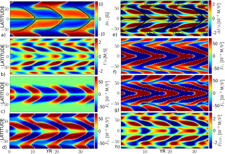
Figure 3: Model M1. a) Time-latitude diagram of the radial magnetic field at the surface (background image) and the toroidal magnetic field at the bottom of the subsurface shear layer (SSL) $r_{s}=0.9R$, the contour lines are plotted in range of $\pm$1kG with exponential decrease of magnitude to the low values of $\pm$4G; b) time-latitude diagram of the torsional oscillations (background image) at the surface; c) azimuthal density force from variations of the turbulent stress at the surface, $F_{\ell}$; d) the same as c) for the large-scale Lorentz force, $F_{L}^{(t)}$; e) time-latitude diagram of the zonal flow acceleration (background image) at the surface and the toroidal magnetic field in the subsurface shear layer (same as panel (a)); f) the same as in panel (d) for the “inertial” forces, $F_{I}$; g) the same as in panel (d) for the effect of the meridional flow, $F_{U}$; h) the total force at the surface, $F_{\mathrm{TOT}}=F_{\ell}+F_{I}+F_{L}^{(t)}+F_{U}$.

We start with describing the full dynamo models that take into account all nonlinear effects, and reproduce the extended mode of the torsional oscillation. Figure 3 shows results for the magnetic field evolution in model M1 at the top boundary of the convection zone together with the corresponding evolution of dynamo-induced zonal variations of the rotational velocity and zonal acceleration, as well as contributions of the zonal force components. The large-scale toroidal magnetic field at the bottom of the subsurface shear layer varies with the magnitude of 1.5 kG. In the subsurface shear layer, the dynamo wave of the toroidal magnetic field starts at about $60^{\circ}$ latitude, approximately 1-2 years after the end of the previous activity cycle. The magnitude of the toroidal magnetic field at this latitude is about 4 G. The wave propagates toward the equator in $\sim 22$ years. The polar and equatorial branches of the dynamo waves are almost completely overlapped in time. The radial magnetic field reveals the extended mode as well. Its evolution is in agreement with the observational results of Stenflo & Guedel (1988) and Stenflo (1992).

The dynamo wave forces variations of the angular velocity and meridional circulation. It is seen in Fig. 3e that the induced zonal acceleration is $\sim 2-4\times 10^{-8}~{}$m s^-2, which is in agreement with the observational results of Kosovichev & Pipin (2019). However, the individual force contributions are by more than an order of magnitude stronger than their combined action. Another interesting finding is that two components of the azimuthal force show the extended 22-year modes. They are: $F_{U}$, associated with variations of the meridional circulation, and the inertial force, $F_{I}$. In model M1, the large-scale Lorentz force, $F_{L}^{(t)}$ displays an extended pattern corresponding to 16 years of drifting to the equator. The equatorial branches of forces, $F_{U}$ and $F_{I}$, are nearly in balance. The effect of magnetic field on the turbulent stress does not show the extended cycle, or it is strongly quenched at high latitudes. However, the total force, $F_{\mathrm{TOT}}=F_{\ell}+F_{I}+F_{L}^{(t)}+F_{U}$, clearly shows the extended mode (Fig. 3h). Its time-latitude pattern corresponds to the zonal acceleration evolution. It is seen that different parts of the zonal acceleration diagram correspond to the different excitation forces. For example, the polar brunch is in phase with $F_{U}$ and $F_{L}^{(t)}$, at mid latitudes the zonal acceleration is in phase with $F_{L}^{(t)}$, at low latitudes it is in phase with $F_{\ell}$, and the equatorial part is in phase with $F_{U}$. It is important that the model takes into account force $F_{U}$, resulting from the nonlinear effects of forces $F_{L}^{(t,p)}$ and $F_{\ell}$ driving the torsional oscillations. Force $F_{I}$ is the restoring inertial force. The results for model M2 with two meridional circulations cells are qualitatively similar to M1.

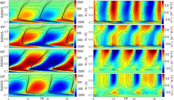
Figure 4: Model M1. Left column shows time-radius diagrams for the toroidal magnetic field evolution (background images, in [G] units) for latitudes from 10^∘ to 60^∘, the radial magnetic field is shown by contours in the range of $\pm 10$G. The right column shows the zonal acceleration (background images) and the azimuthal velocity variations (shown by contours in the range of $\pm 3~{}$m/s.)

Figure 4 shows the time-radius diagrams of the evolution of the large-scale magnetic field and flows in model M1 for four latitudes, 10^∘, 30^∘, 45^∘, and 60^∘. The large-scale magnetic field migrates in two directions: upward in the main part of the convection zone, and downward near the bottom of the convection zone and in the tachocline. Generally, direction of propagation of the torsional oscillations corresponds to propagation of the dynamo wave at both, the high and low latitudes. At 60^∘ latitude, the inclination of the torsional wave pattern in the time-radius diagram is small, and variations of the zonal acceleration are synchronized by the phase at all depths of the solar convection zone. At lower latitudes, the torsional waves propagate upward from the bottom of the convection zone, and form almost stationary oscillatory patterns in the subsurface layer, the depth of which increases with the latitude decrease. These effects qualitatively correspond to the results of our recent helioseismology analysis (Kosovichev & Pipin, 2019).

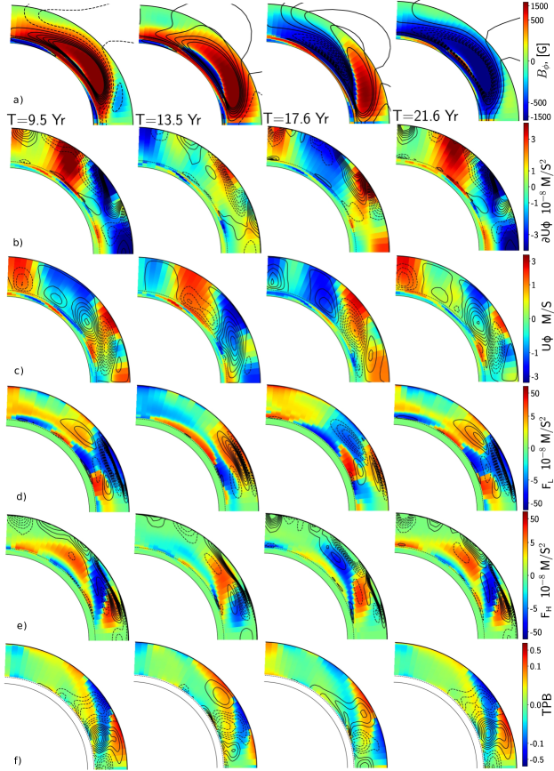
Figure 5: Model M1. Snapshots for a half of dynamo cycle of: a) the toroidal magnetic field (background image) and streamlines of the poloidal field (contours); b) variations of the zonal acceleration (background image) and the azimuthal force caused by variations of the meridional circulation, $F_{U}$, (contour lines are plotted in the range $\pm 50$ m/s²); c) variations of the azimuthal velosity and contours show streamlines of the variations of meridional circulation, dashed lines are for the counter clockwise circulation; d) the azimuthal force caused by the Lorentz force $F_{L}^{(t)}$ (background image) and the magnetic quenching of the turbulent angular momentum transport $F_{\ell}$ (contours in the range of $\pm 50$ m/s²); e) the dynamo-induced $\Lambda$-effect, $F_{H}$, the term $H^{(0,\rho)}$ (background image), see Eqs (20), and contours (in the range $\pm 50$ m/s²) show variations of the inertial forces, $F_{I}$; e) contours, in range of $\pm 5\cdot 10^{-3}$, show the relative variations of the convective flux, $\delta F_{c}/F_{\odot}$ , where $F_{\odot}$ is the total energy flux, background image shows the relative variations of the Taylor-Proudman balance (TPB); TPB includes all terms of the right-hand side of Eq. (2.1) except the advection term. To display the whole range of the TPB variations we use normalization to unity and the logarithmic scale

Figure 5 shows the evolution of the large-scale magnetic field, flows, the dynamo-induced forces variations of convective flux $\delta F_{c}/F_{\odot}$ (where $F_{\odot}$ is the total energy flux), and variations the Taylor-Proudman balance (TPB) inside the convection zone in model M1. The TPB includes all terms of the right hand side of Eq. (2.1) except the advection term. The results for model M2 are very similar. Both models show the qualitatively similar results despite the different meridional circulation structure in the convection zone. The secondary deep clockwise meridional cell of magnitude 1 m/s is weak, and does not significantly affects the dynamo wave propagation in model M2. In both models, M1 and M2, the maximum of the toroidal magnetic field strength near the bottom of the convection zone is about 5 kG. The strength of the toroidal magnetic field drops to about 1 kG at $0.9R$. At low latitudes, the dynamo wave propagates to the equator, upward in the upper part of the convection zone and downward in the tachocline. At high latitudes, there is a poleward propagating branch, which has a rather weak signature at the surface. It is also seen in the time-latitude diagrams of the toroidal magnetic field in the subsurface layers, (see, Fig. 3).

A new dynamo cycle starts near the bottom of the convection zone at about 60 degrees latitude in the region subjected to the zonal deceleration. The acceleration pattern in the upper part of the convection zone drifts toward equator following the propagation of the dynamo wave (see, Fig. 5a,b). Figures 5d,e shows that the zonal deceleration is ahead of the toroidal magnetic field due to the combined effect of the large-scale Lorentz force, $F_{L}^{(t)}$, and the dynamo induced $\Lambda$-effect, $F_{H}$. Notably, the $F_{H}$ force migrates closer to the equator than the $F_{L}^{(t)}$ force. The forces $F_{U}$ (Fig. 5b) and $F_{I}$ (Fig. 5e) are opposite in sign, and they have similar latitudinal structures. We see that in the latitude range from 50^∘ to 60^∘, where the extended dynamo mode is initiated, the acceleration is provided by the inertia force, $F_{I}$ (Figs. 5b and e). Also, we see that, during a half of the extended torsional oscillation cycle, effects of $F_{U}$, $F_{L}$ and $F_{H}$ are synchronized in the subsurface layer of the convection zone. The polar branch of the torsional oscillations in model M1 is due to effects of the Lorentz force and variations of the meridional circulation. The models show weak meridional circulation variations in the main part of the convection zone, where its magnitude is about 10–20 cm/s. The surface variations of the meridional circulation in the dynamo cycle are about 1 m/s. Figure 5c shows that the direction of the excited meridional flow, which migrates to the equator ahead of the toroidal magnetic field, is counter-clockwise (poleward on the surface), and that it is clockwise for the flow behind. This corresponds to the meridional flow variations converging towards the activity belts in agreement with results of local helioseismology (Komm et al., 2012; Zhao et al., 2014; Kosovichev & Zhao, 2016).

Figure 5f shows variations of the convective flux $\delta F_{c}/F_{\odot}$, where $F_{\odot}$ is the total energy flux, and the relative variations the Taylor-Proudman balance (TPB) inside the convection zone in model M1. We see that the large-scale toroidal magnetic field results in a reduction of the convective flux. This phenomenon, called the magnetic shadow effect, was discussed earlier by, e.g., Brandenburg et al. (1992) and Pipin (2004), and is usually considered in the problem of the solar-cycle luminosity variation. In the model, the magnetic shadow effect induces variation of the latitudinal gradient of the mean entropy. This results in perturbation of the Taylor-Proudman balance and variations of the meridional circulation. In agreement with other studies, e.g. of Durney (1999), Rempel (2006) and Miesch et al. (2011), the variations of TPB are concentrated near the boundaries of the convection zone, and correlate well with $\delta F_{c}/F_{\odot}$. Therefore, the magnetic shadow effect is the main source of the TPB and meridional circulation perturbations in our model. This was also confirmed in separate runs when we switched off all other source of the TPB variations in Eq. (2.1).

Interestingly, a better agreement with the observed extended pattern of the torsional oscillations is found in the special cases of model M1, which are represented by models M4 and M5 in Table 1. In model M4, the influence of the magnetic field on the angular momentum is restricted to effect of the large-scale Lorentz force, $F_{L}^{(t)}$, and $F_{\ell}$, associated with the small-scale Maxwell stresses $\overline{b_{i}b_{j}}/4\pi\overline{\rho}$ is neglected. In model M5, which is probably in the best agreement, the $F_{L}^{(t)}$ effect is neglected, and the torsional oscillations are driven by $F_{\ell}$. Model M6 uses the same approach as M5 but it employs the dynamo-induced $\Lambda$-effect of a different origin (see, Table 1). This model does not show the extended mode of the torsional oscillation.

3.2 Effect of the extended dynamo mode and cycles overlap

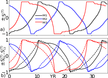
Figure 6: a) The relative area occupied by the toroidal magnetic flux of one sign at the bottom of the subsurface shear layer, $\mathrm{S^{(T)}}$, in models M1, M2 and M3; b) the same as (a) for the parameters $\mathrm{S_{SSL}^{(T)}}$(solid lines) , and $\mathrm{S_{CZ}^{(T)}}$ (dashed lines).

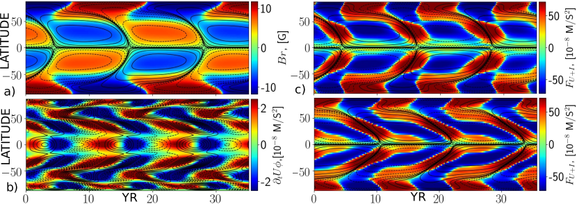
Figure 7: Model M3. a) Time-latitude diagram of the radial magnetic field at the surface (background image) and the toroidal magnetic field at the bottom of the subsurface shear layer b) the time-latitude diagram of the zonal flow acceleration (background image) at the surface and the zonal velocity variations (contours in range of $\pm 3$m/s); c) the time-latitude diagram of $F_{I}+F_{U}$ (background image) for model M3; d) the same as c) for model M1, for comparison.

Both models, M1 and M2, (with the single- and double-cell meridional circulation) show the extended mode of the torsional oscillations. It seems natural to relate this effect with extended dynamo mode which shows up in these models. On the Sun, this dynamo mode is deduced from the overlap of magnetic cycles (Stenflo, 1992). To quantify the overlap in our models, we use the parameters of the toroidal magnetic field distributions (Eqs. 21-23). To demonstrate the role of the extended dynamo mode and the cycle overlap, we consider model M3 with anisotropy of the turbulent eddy-diffusivity, following results of Pipin & Kosovichev (2014). The anisotropy is controlled by parameter $\eta_{A}$, see Eq. (2.2). In model M3, we put $\eta_{A}=2\eta_{T}$. This decreases the overlap of the subsequent cycles. Figure 6 shows evolution of the parameters, $\mathrm{S^{(T)}}$, $\mathrm{S_{SSL}^{(T)}}$, and $\mathrm{S_{CZ}^{(T)}}$, for models M1, M2 and M3. Figure 6(a) shows that, at the bottom of the subsurface shear layer, the dynamo waves of the toroidal magnetic field are not fully overlap in all models, and that the time delay between the end of a magnetic cycle at the equator, and the start of a new cycle at high latitudes is about 1.2 years in model M1, 1.1 years in model M2, and 2.5 years in model M3. However, in terms of the magnetic flux integrated over the subsurface shear layer or over the bulk of the convection zone, we find that in models M1 and M2 the dynamo waves are overlapped because $\mathrm{S_{SSL}^{(T)}}$, and $\mathrm{S_{CZ}^{(T)}}\sim 0.96$ . Model M3 shows a time delay of about 1.5 year for the dynamo waves in the convection zone (Fig. 7a).

The delay between the subsequent cycles in the subsurface shear layer results in an interruption of the torsional oscillation pattern in the equatorial regions (Fig 7b). The sum of the forces, $F_{I}+F_{U}$, that form the main balance and drive the extended mode of the torsional oscillations in models M1 (Fig. 7d) and M2, but not in model M3 (Fig 7c). Therefore, the decrease of the dynamo-cycle overlap breaks the phase continuity in the balance of forces driving the torsional oscillations. The cycle overlap can interpreted as a measure of penetrations of the toroidal magnetic field from the deep convection zone into the subsurface shear layer in course of the magnetic cycle. The additional anisotropy of magnetic diffusivity in model M3 disperses magnetic field in the radial direction (Pipin & Kosovichev, 2014), and, thus, reduces penetration of the toroidal from the convection zone to the surface.

3.3 Magnetic perturbations of the convective heat flux and meridional circulation

Our results presented in the previous sections, showed that the dynamo-induced variations of the meridional circulation play a significant role in the total force balance driving the torsional oscillations. This effect results from the torque induced by the large-scale flows, $-\boldsymbol{\nabla\cdot}\left(r\sin\theta\overline{\rho}\overline{U}_{\phi}\mathbf{\overline{U}^{m}}\right)$, where $\overline{U}_{\phi}=r\sin\theta\Omega$, and $\mathbf{\overline{U}^{m}}$ is the meridional circulation velocity. Generally, $\left|\overline{U}_{\phi}\right|\gg\left|\mathbf{\overline{U}^{m}}\right|$. The dynamo-induced perturbations of the angular velocity are of the same order of magnitude as the perturbation of the meridional circulation. Therefore, the leading term of the torque driving the torsional oscillations can be written as: $-\boldsymbol{\nabla\cdot}\left(r\sin\theta\overline{\rho}\overline{U}_{\phi}\mathbf{\delta\overline{U}^{m}}\right)$, where $\mathbf{\delta\overline{U}^{m}}$ is the dynamo-induced perturbation of the meridional circulation velocity. In the middle of the convection zone: $\mathbf{\delta\overline{U}^{m}}\sim$10 cm/s, $\overline{U}_{\phi}\sim 2.5$ km/s. Therefore, the effect of this perturbation is comparable with the speed of the torsional oscillations, 5-10 m/s.

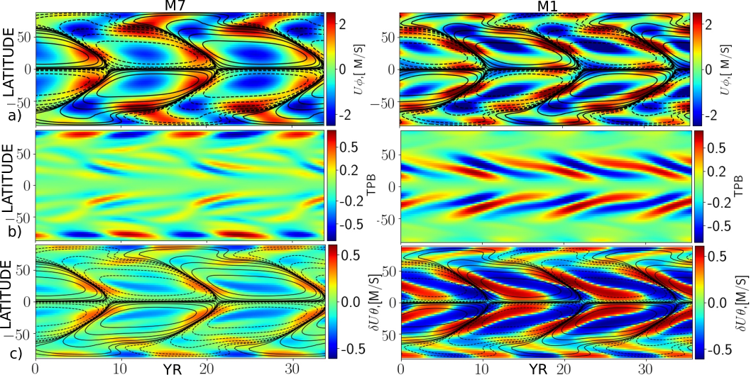
Figure 8: Model M7 (left column) and model M1 (right column). a) Time-latitude diagram of the mean toroidal magnetic field in the subsurface shear layer $r=0.9-0.99R$ (contour lines are plotted in range of $\pm$1kG with exponential decrease of magnitude to the low values of $\pm$4G and the time-latitude diagram of the azimuthal velocity oscillations (background image) at the surface; b) the dynamo induced relative variations of the Taylor-Proudman balance at the surface; c) the time-latitude diagram of the toroidal magnetic field (same as in panel a) and variations of the meridional circulations at the surface; positive variations mean the poleward flow.

Variations of meridional circulation are caused by perturbations of the Taylor-Proudman balance (TPB). Results for model M1 show that, near the surface, perturbations of the TPB correlate with variations of the convective flux, $\delta F_{c}/F_{\odot}$, which are caused by quenching of the convective heat flux by the large-scale magnetic field. The impact of this effect on the torsional oscillations is demonstrated by comparison of models M1 and M7 (Fig. 8). In model M7, the magnetic quenching of convective flux is neglected. This model does not show the extended mode of torsional oscillations. Variations of the TPB and meridional circulation in model M7 are substantially smaller in magnitude than in model M1 and they disagree with observations. The time-latitude diagram of the meridional circulation variations in model M1 is in a good agreement with observations (Komm et al., 2012; Zhao et al., 2014; Kosovichev & Zhao, 2016). To check the role of variations of the meridional circulation we made a special run, in which we suppressed the variations, and obtained the results similar to model M7 (Fig. 8a), without the extended torsional oscillation pattern.

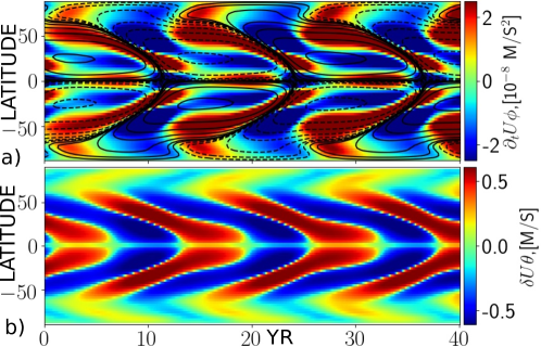
Figure 9: Model M8. a) Time-latitude diagram of the mean toroidal magnetic field in the subsurface shear layer (contour lines are plotted in range of $\pm$1kG with exponential decrease of magnitude to the low values of $\pm$4G) and the time-latitude diagram of the azimuthal velocity acceleration (background image) at the surface; b) variations of the meridional circulations at the surface; positive variations mean the poleward flow.

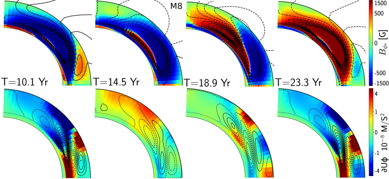
Figure 10: Model M8. a) Snapshots of the toroidal magnetic field and streamlines of the poloidal magnetic field; b) snapshots of the zonal accelerations (background images) and the streamlines of the meridional circulation variations; amplitude of the meridional circulation variation is about $\pm 1$m/s.

In model M8, we switch off effects of the large-scale Lorentz force, $F_{L}^{(t,p)}=0$, and the Maxwell stresses contribution of the small-scale magnetic fields, $F_{\ell}=0$, and $F_{H}=0$. In this case, the torsional oscillation are driven by magnetic quenching of the convective heat flux. This effect was previously discussed using the heuristic arguments by Spruit (2003) and Rempel (2006). In our models, we employ analytical results of the mean-field theory using expressions for the thermal eddy conductivity tensor, given by Eq. (A13) for the case of rotating and magnetized fluid (Kitchatinov et al., 1994; Pipin, 2018). The time-latitude diagram of the toroidal magnetic field, the azimuthal velocity acceleration and variations of the meridional circulation are shown in Figure 9, and the snapshots for the different phases of the magnetic cycle are shown in Figure 10. This model shows the extended cycle of the torsional oscillations. Except the polar region parts, the torsional oscillation pattern is similar to results of the model M4. The polar parts, in turn, are qualitatively similar to model M5. Like in model M1, variations of the meridional oscillations are in agreement with the results of observations. The results for this model show that the effect of large-scale magnetic field on the convective heat transport is among significant drivers of the solar torsional oscillations.

4 Discussion and conclusions

Our paper addressed the question of the origin of the solar torsional oscillations, and, in particular, its extended 22-year mode. We presented a non-linear mean-field dynamo model that self-consistently describes the differential rotation and meridional circulation, as well as the generation and transport of the large-scale magnetic field. For the first time, the model explains the phenomenon of the extended solar cycle observed in the torsional oscillation pattern, and reveals the balance of forces that drive the torsional oscillations.

The model is based on the mean-field magnetohydrodynamics theory of turbulent generation of large-scale magnetic field, as well as turbulent heat and angular momentum transport. We employ the reference state computed from the standard evolutionary model of the Sun, and use turbulent parameters of the convective RMS velocity to calculate the mean-field non-diffusive turbulent effects and heat transport. The angular momentum transport in the convection zone is affected by the large-scale Lorentz force and magnetic effects on the turbulent stress tensor, $\hat{T}_{\mathrm{ij}}=\overline{u_{i}u_{j}}-\overline{b_{i}b_{j}}/4\pi\overline{\rho}$. The turbulent stresses cause generation and dissipation of the large-scale flows (see Eq. A2). The dynamo-generated magnetic field results in quenching of the turbulent angular momentum fluxes as well as the non-dissipative angular momentum flux, which in terms of the mean-field theory is described as the $\Lambda$-effect. In the case of the weak mean field, its amplitude is proportional to $\overline{B}^{2}$. Our model describes the dynamo processes distributed in the convection zone.

Previous models of the torsional oscillations were constructed by coupling the dynamo equations with equations of the angular momentum transport (e.g. Malkus & Proctor, 1975; Kueker et al., 1996; Pipin, 1999; Küker et al., 1999; Covas et al., 2000). However, such models did not describe the angular momentum flux induced by variations of the meridional circulation. These variations naturally result from perturbations of the Taylor-Proudman balance, and are caused by the dynamo-induced variations of the centrifugal force, variations of the “thermal wind” (associated with the mean entropy gradient), magnetic quenching of the eddy-viscosity and the large-scale Lorentz force. Dynamo-induced perturbations of the Taylor-Proudman balance in the framework of the mean-field theory were previously considered by Brandenburg et al. (1992) and Rempel (2007). Therefore, it is important that the nonlinear consistent dynamo models presented in this paper describe both, the differential rotation and the meridional circulation, as well as their variations.

We find two essential conditions that affect excitation of the extended mode of the torsional oscillations in the large-scale dynamo operating in the bulk of the convection zone. They are as follows: a) the existence of the extended mode in the dynamo wave pattern and overlap of subsequent dynamo waves in the time-latitude diagram; b) the dynamo-cycle variations of the meridional circulation which stem from quenching the convective heat transport by the large-scale magnetic field. This effect is called the magnetic shadow (Stix, 2002). It represents a mean-field analog of the phenomenon observed in sunspots (Kitchatinov et al., 1994). Condition (a) is related to the distribution of the dynamo process inside of the convection zone. Our models show that the dynamo waves extent over the depth of the convection zone and over latitudes from the equator to polar regions. The magnetic forces are distributed similarly (e.g., the snapshots of the large-scale Lorentz force, $F_{L}^{(t)}$ and the dynamo induced $\Lambda$-effect, $F_{H}$, in Fig. 5c and d.) This is different to the flux-transport models, where the dynamo wave occupies only a particular range of depth, near and below the bottom of the convection zone (e.g. Choudhuri & Dikpati, 1999; Rempel, 2006). To demonstrate the importance of this condition we calculated a dynamo model that includes effects of anisotropy of background convective flows on the eddy diffusivity in a parametric form (Pipin & Kosovichev, 2014). This modification restricts the latitudinal extent of the dynamo wave, reduces the overlap of the subsequent cycles, and results in disappearance the extended mode of the torsional oscillations. Inspection of results for the other models (see, the Table 2) shows that the cycle overlap depends on the nonlinear effects which take part in the magnetic field evolution.

The importance of condition (b) – the dynamo-induced variations of the convective flux that results in the meridional circulation variations – is confirmed by results of model M7 where these variations were suppressed. Coupling with variations of the Taylor-Proudman balance, the variations of the meridional circulation affect the amplitude of the torsional oscillations and produce the effective drifts of the torsional wave in radius and latitude. Our modeling results showed that neglecting the meridional circulation variations results in disconnections in the torsional oscillation patterns near the bottom of the convection zone and at the surface. In our model, the greatest effect on the TPB results from variations of the mean entropy caused by variations of the convective heat transport. Thus, neglecting this effect, as shown in model M7, results in no extended mode of the torsional oscillations.

Results of our models show that the evolutionary pattern of the torsional waves can depend on the physics involved in the effects of magnetic field on the angular momentum transport (see, Eqs 14-19). These effects are usually considered as the principal sources of the 11-year modulations of zonal flows in sunspot cycles. We find that the extended mode of the torsional oscillations can be qualitatively explained in different ways, either by combination of the magnetic feedback on the turbulent fluxes of the angular momentum transport, the $F_{\ell}$ and $F_{H}$ forces (called the $\Lambda$-quenching), and the large-scale Lorentz force, $F_{L}^{(t)}$, as in model M1, or by separate actions by the large-scale Lorentz force (model M4) and the $\Lambda$-effect quenching (model M5). The results of global MHD models of Guerrero et al. (2016a) and Käpylä et al. (2016) show significance of the large-scale Lorentz force for evolution of the high-latitude branches of the torsional oscillations. This is also found in our models M1 and M4.

It is interesting that in both models, M4 and M5, the magnetic drivers of the torsional oscillations are related to the forces which reduce the large-scale latitudinal shear. Model M6 employs the dynamo induced $\Lambda$-effect, $H^{(0,a)}$ which is caused by the anisotropy of background convective flows. This effect works to increase the latitudinal shear. However it does not produces the extended mode.

The robustness of our conclusions depends on the radial distribution of the large-scale field, which determines the zonal flow acceleration in the convection zone. Comparing results of our model with observations (Fig. 1), we see that in our models the latitudinal width of the zonal flow acceleration pattern is somewhat smaller than in the observations . The models show axially aligned zonal acceleration patterns at mid latitudes (Fig. 5). The observations show a slightly different inclination of these patterns (e.g., Figure 2 in Kosovichev & Pipin, 2019). The near-equatorial structure of the torsional oscillations is in agreement with the observations, as well as variations of the meridional circulation.

Summing up, it is found the extended 22-yr mode of the solar torsional oscillations (zonal flow variations) can be explained by effects of the overlapped dynamo waves on the angular momentum and heat transport in the solar convection zone. The possible scenario of the extended cycle of solar torsional oscillations is as follows. At high latitudes, the torsional wave is excited by the large-scale Lorentz force with contributions from the dynamo-induced $\Lambda$-effect and the magnetic quenching of the convective heat flux. Then, the wave propagates towards the equator. Near the equator, the large-scale Lorentz force and the dynamo-induced $\Lambda$-effect are about zero. However, the toroidal magnetic field in the near-equatorial (sunspot formation) zone results in quenching of the convective heat flux. This induces variations of meridional flows from the polar and equatorial sides to the central part of the sunspot formation zone. These flows slow down the equatorial side of the dynamo wave, moving the torsional wave closer to the equator. This meridional circulation effect operates during the active phase of the cycle. Taking into account the overlap of the dynamo waves, we explain the extended pattern of the torsional waves.

Table 1: Model parameters: $\eta_{A}$ controls the anisotropic eddy diffusivity (see, Eq. 2.2); $\ell_{\mathrm{min}}$ controls the number of meridional circulation cells along the radius; columns $F_{U}$, $F_{\ell}$, $F_{L}^{(\mathrm{t,p})}$, and $F_{H}$ show the nonlinear and dynamic effects involved in the angular momentum balance; contribution $H^{(0,a)}$ stems from anisotropy of convective turbulence, and $H^{(0,\rho)}$ results from the density stratification (see the text).

Model	$\eta_{A}$	$\mathrm{\ell_{min}}/R$	N Cells	$F_{U}$	$F_{\ell}$	$F_{L}^{(\mathrm{t,p})}$	$\mathrm{\chi_{ij}}$(Eqs(3,A13))	$F_{H}$
M1	0	$0.02$	1	Y	Y	Y	$\mathrm{\chi_{ij}\left(\Omega^{\star},\beta\right)}$	$H^{(0,\rho)}$
M2	0	0.01	2	-/-	-/-	-/-	-/-	$H^{(0,\rho)}$
M3	2$\eta_{T}$	0.02	1	-/-	-/-	-/-	-/-	$H^{(0,\rho)}$
M4	0	0.02	1	Y	N	Y	-/-	0
M5	0	-/-	1	Y	Y	N	-/-	$H^{(0,\rho)}$
M6	0	-/-	1	Y	Y	N	$\mathrm{\chi_{ij}\left(\Omega^{\star},\beta\right)}$	$H^{(0,a)}$
M7	0	-/-	1	Y	Y	Y	$\mathrm{\chi_{ij}\left(\Omega^{\star}\right)}$	$H^{(0,\rho)}$
M8	0	0.02	1	Y	N	N	$\mathrm{\chi_{ij}\left(\Omega^{\star},\beta\right)}$	0

Table 2: Model properties: the dynamo cycle period, the delay between the subsequent cycles (see the main text), duration of the extended dynamo mode, magnitudes of the torsional oscillation velocity and zonal acceleration on the surface, duration of the equatorial branch of the extended mode of the torsional oscillations, duration of the polar branch of the torsional oscillations.

Observ./ Model	Cycle Period, [yr]	Cycle’s $\Delta t$, [yr]	Dynamo Ext. mode Length, [yr]	$\delta U_{\phi}$ [M/S]	$\partial_{t}U_{\phi}$ $10^{-8}$[M/S2]	Ext. mode, [yr]	Polar branch, [yr]
Observ.	22		20		$\pm 8$	20	9
M1	22.9	1.2	21.7	$\pm 4.3$	$\pm 5.6$	24.	8
M2	20.6	1.1	19.2	$\pm 4.7$	$\pm 7.1$	22	7.8
M3	23.4	2.6	23.5	$\pm 2.7$	$\pm 4.5$	N	6
M4	24.5	1.2	25.1	$\pm 3$	$\pm 6.8$	25.1	10
M5	22.6	0.9	23.8	$\pm 4$	$\pm 7$	20	8.1
M6	20.1	0.9	20.1	$\pm 5.7$	$\pm 14.2$	N	5
M7	25	1.8	26.3	$\pm 2.7$	$\pm 4.4$	N	9
M8	25.1	1.7	25	$\pm 4$	$\pm 7$	23.1	8.3

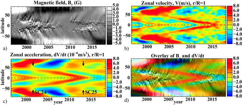
Figure 1: Observational results from SoHO/MDI and SDO/HMI. The time-latitude diagrams of: a) evolution of radial magnetic field during the last two solar cycles; b) zonal flow velocity (‘torsional oscillations’); c) zonal acceleration calculated after applying a Gaussian spatial and temporal filter, arrows indicate the start of extended solar cycles 24 and 25 at about 55 degrees latitude, defined as a starting point of the zonal deceleration (blue ares); d) overlay of the zonal acceleration (color image) and the radial magnetic field (gray-scale) (after Kosovichev & Pipin, 2019).

.

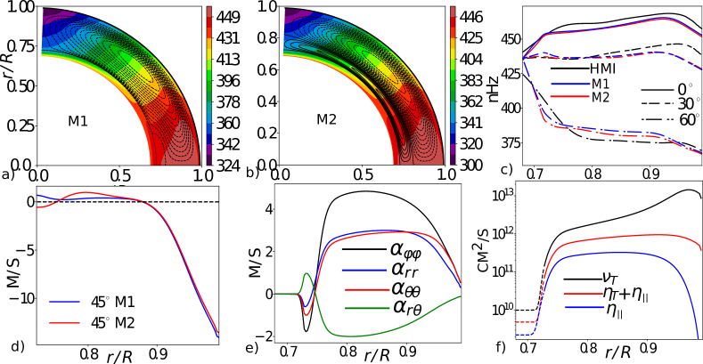
Figure 2: The angular velocity and meridional circulation distributions for the models specified in Table 1: a) model M1; b) model M2; c) radial profiles of the angular velocity at 0, 30 and 60 degrees latitudes ( blue for model M1, red - M2), and obtained from the SDO/HMI helioseismology data archive (black); d) radial profiles of the meridional circulation velocity at latitude 45^∘; e) radial profiles of the $\alpha$-effect tensor at latitude 45^∘; f) radial profiles of the isotropic part of the eddy viscosity, $\nu_{T}$, the total, $\eta_{T}+\eta_{||}$, and rotationally induced part, $\eta_{||}$, of the eddy magnetic diffusivity.

Appendix A Model Details

A detailed description of the mean-field solar dynamo model, as well as the model for the angular momentum balance and heat transport, can be found in our previous papers (Pipin, 2018; Pipin & Kosovichev, 2018). Here, we collect analytical results on the magnetic field contribution to the $\Lambda$-effect. This contribution is a part of the turbulent stress tensor

$${\hat{T}_{ij}=\left(\left\langle u_{i}u_{j}\right\rangle-\frac{1}{4\pi\overline{\rho}}\left(\left\langle b_{i}b_{j}\right\rangle-\frac{1}{2}\delta_{ij}\left\langle\mathbf{b}^{2}\right\rangle\right)\right),}$$ (A1)

where $\mathbf{u}$ and $\mathbf{b}$ are fluctuating velocity and magnetic fields. Application the mean-field hydrodynamic framework (see, Kitchatinov et al. 1994) leads to the Taylor expansion in terms of the scale-separation parameter $\ell/L$:

$$\hat{T}_{ij} = \hat{T}_{ij}^{\left(\Lambda\right)}+\hat{T}_{ij}^{\left(\nu\right)}$$ (A2)

$$= \Lambda_{ijk}\Omega_{k}-N_{ijkl}\frac{\partial\overline{U}_{k}}{\partial r_{l}}+\dots$$ (A3)

The non-diffusive flux of angular momentum $\boldsymbol{\Lambda}=\left\langle{u}_{\phi}^{\prime}{\boldsymbol{u}}\right\rangle$ can be expressed as follows (Ruediger, 1989):

$$\hat{T}_{r\phi}^{\left(\Lambda\right)} = \Lambda_{V}\Omega\sin\theta,$$

$$\Lambda_{V} = \nu_{T}\left(V^{(0)}+\sin^{2}\theta V^{(1)}\right),$$ (A4)

$$\hat{T}_{\theta\phi}^{\left(\Lambda\right)} = \Lambda_{H}\Omega\cos\theta,$$

$$\Lambda_{H} = \nu_{T}\left(H^{(0)}+\sin^{2}\theta H^{(1)}\right)$$ (A5)

In the previous papers, we discuss in detail the standard parts of this parametrization for coefficients $V^{(0)}$, $V^{(1)}$ and $H^{(1)}$. It was shown that the analytical form of the $\Lambda$-effect coefficients becomes fairly complicated if we wish to account for the multiple-cell meridional circulation structure. Also, results of Pipin & Kosovichev (2018) show that the spatial derivative of the Coriolis number $\Omega^{*}=2\Omega_{0}\tau_{c}$, has to be taken into account.

In our nonlinear models, we take into account the effect of magnetic field (see, Pipin 1999), as well as the effect of convective velocities anisotropy, which is important for modeling the subsurface shear layer. Therefore, the final coefficients of the $\Lambda$-tensor are:

$$V^{(0)} = \Bigl{[}\left(\frac{\alpha_{MLT}}{\gamma}\right)^{2}\left\{J_{0}+\!J_{1}+\!a\left(I_{0}+\!I_{1}\right)\right\}$$

$$- \Bigl{(}\frac{\alpha_{MLT}\ell}{\gamma}\frac{\partial}{\partial r}\left\{\left(J_{0}+J_{1}\right)-I_{5}+I_{6}\right\}+\ell^{2}\frac{\partial^{2}}{\partial r^{2}}\left(I_{1}-I_{2}\right)\Bigr{]}\phi_{\chi}^{(I)}\left(\beta\right),$$

$$V^{(1)} = -\left\{\left(\frac{\alpha_{MLT}}{\gamma}\right)^{2}\left(J_{1}+aI_{1}\right)-\frac{\alpha_{MLT}\ell}{\gamma}\frac{\partial}{\partial r}\left(J_{1}+I_{6}\right)-\ell^{2}\frac{\partial^{2}}{\partial r^{2}}I_{2}\right\}\phi_{\chi}^{(I)}\left(\beta\right),$$ (A7)

and ${H^{(1)}=-V^{(1)}}$. We introduce the anisotropy parameter, $a={\displaystyle\frac{\overline{u_{h}^{2}}-2\overline{u_{r}^{2}}}{\overline{u_{r}^{2}}}=}2$, where $u_{h}$ and $u_{r}$ are the horizontal and vertical RMS velocities. Collecting results of Kitchatinov et al. (1994) and Kueker et al. (1996), we write the coefficient, $H^{(0,\rho)}$, as follows:

$$H^{(0,\rho)} = \frac{\tau^{2}\left\langle\boldsymbol{u}^{\prime 2}\right\rangle}{\rho^{2}}\phi_{H}\left(\beta\right)\frac{\partial^{2}}{\partial r^{2}}\left(\rho^{2}J_{4}\right)$$

$$= \left\{4\left(\frac{\alpha_{MLT}}{\gamma}\right)^{2}J_{4}-4\frac{\alpha_{MLT}\ell}{\gamma}\frac{\partial}{\partial r}J_{4}+\ell^{2}\frac{\partial^{2}}{\partial r^{2}}J_{4}\right\}\phi_{H}\left(\beta\right),$$

where function $J_{4}$ was defined by Kitchatinov et al. (1994), and the magnetic quenching function $\phi_{H}\left(\beta\right)$ was defined by Pipin (2003):

$$\phi_{H} = \frac{1}{\beta^{2}}\left(\frac{2+3\beta^{2}}{2\sqrt{\left(1+\beta^{2}\right)^{3}}}-1\right).$$ (A9)

The magnetically induced $\Lambda$-effect caused by the turbulence anisotropy was discussed by Kichatinov (1988). Following his results, we define:

$$H^{(0,a)} = \left(\frac{\alpha_{MLT}}{\gamma}\right)^{2}aJ_{H}\left(\beta\right)J_{3}\left(\Omega^{*}\right)$$ (A10)

where

$$J_{H} = \frac{105}{256\beta^{4}}\left(\beta^{2}-37-\frac{8}{1+\beta^{2}}+\left(\beta^{4}+6\beta^{2}+45\right)\frac{\arctan\beta}{\beta}\right),$$ (A11)

$$J_{3} = \frac{9}{15\Omega^{*6}}\left(15+\Omega^{*2}+\left(\Omega^{*4}-6\Omega^{*2}-15\right)\frac{\arctan\Omega^{*}}{\Omega^{*}}\right).$$ (A12)

The convective heat transport is treated in the same way as in the recent paper of Pipin (2018). For expressions of the eddy heat conductivity tensor we employ the following expression:

$$\chi_{ij}=\chi_{T}\left(\phi_{\chi}^{(I)}\left(\beta\right)\phi\left(\Omega^{*}\right)\delta_{ij}+\phi_{\chi}^{(\|)}\left(\beta\right)\phi_{\parallel}\left(\Omega^{*}\right)\frac{\Omega_{i}\Omega_{j}}{\Omega^{2}}\right),$$ (A13)

where functions $\phi$ and $\phi_{\parallel}$ were defined in Kitchatinov et al. (1994), and the magnetic quenching functions $\mathrm{\phi_{\chi}^{(I)}}$ and $\phi_{\chi}^{(\|)}$ are

$$\mathrm{\phi_{\chi}^{(I)}} \mathrm{=} \mathrm{\frac{2}{\beta^{2}}\left(1-\frac{1}{\sqrt{1+\beta^{2}}}\right),}$$

$$\phi_{\chi}^{(\|)} = \mathrm{\frac{2}{\beta^{2}}\left(\sqrt{1+\beta^{2}}-1\right).}$$

References

- Altrock et al. (2008) Altrock, R., Howe, R., & Ulrich, R. 2008, in Astronomical Society of the Pacific Conference Series, Vol. 383, Subsurface and Atmospheric Influences on Solar Activity, ed. R. Howe, R. W. Komm, K. S. Balasubramaniam, & G. J. D. Petrie, 335
- Altrock (1997) Altrock, R. C. 1997, Sol. Phys., 170, 411, doi: 10.1023/A:1004958900477
- Beaudoin et al. (2013) Beaudoin, P., Charbonneau, P., Racine, E., & Smolarkiewicz, P. K. 2013, Sol. Phys., 282, 335, doi: 10.1007/s11207-012-0150-2
- Bekki & Yokoyama (2017) Bekki, Y., & Yokoyama, T. 2017, ApJ, 835, 9, doi: 10.3847/1538-4357/835/1/9
- Böning et al. (2017) Böning, V. G. A., Roth, M., Jackiewicz, J., & Kholikov, S. 2017, ApJ, 845, 2, doi: 10.3847/1538-4357/aa7af0
- Brandenburg (2005) Brandenburg, A. 2005, Astrophys. J., 625, 539
- Brandenburg et al. (1991) Brandenburg, A., Moss, D., Rüdiger, G., & Tuominen, I. 1991, Geophysical & Astrophysical Fluid Dynamics, 61, 179, doi: 10.1080/03091929108229043
- Brandenburg et al. (1992) Brandenburg, A., Moss, D., & Tuominen, I. 1992, A&A, 265, 328
- Cameron & Schüssler (2017) Cameron, R. H., & Schüssler, M. 2017, A&A, 599, A52, doi: 10.1051/0004-6361/201629746
- Choudhuri & Dikpati (1999) Choudhuri, A. R., & Dikpati, M. 1999, Sol. Phys., 184, 61
- Covas et al. (2000) Covas, E., Tavakol, R., Moss, D., & Tworkowski, A. 2000, A&A, 360, L21
- Dikpati & Charbonneau (1999) Dikpati, M., & Charbonneau, P. 1999, ApJ, 518, 508, doi: 10.1086/307269
- Durney (1999) Durney, B. R. 1999, ApJ, 511, 945, doi: 10.1086/306696
- Guerrero et al. (2016a) Guerrero, G., Smolarkiewicz, P. K., de Gouveia Dal Pino, E. M., Kosovichev, A. G., & Mansour, N. N. 2016a, ApJ, 828, L3, doi: 10.3847/2041-8205/828/1/L3
- Guerrero et al. (2016b) —. 2016b, ApJ, 819, 104, doi: 10.3847/0004-637X/819/2/104
- Howe et al. (2018) Howe, R., Hill, F., Komm, R., et al. 2018, ApJ, 862, L5, doi: 10.3847/2041-8213/aad1ed
- Howe et al. (2011) —. 2011, Journal of Physics Conference Series, 271, 012074, doi: 10.1088/1742-6596/271/1/012074
- Jouve et al. (2008) Jouve, L., Brun, A. S., Arlt, R., et al. 2008, A&A, 483, 949, doi: 10.1051/0004-6361:20078351
- Käpylä et al. (2016) Käpylä, M. J., Käpylä, P. J., Olspert, N., et al. 2016, A&A, 589, A56, doi: 10.1051/0004-6361/201527002
- Käpylä (2019) Käpylä, P. J. 2019, A&A, 622, A195, doi: 10.1051/0004-6361/201732519
- Kichatinov (1988) Kichatinov, L. L. 1988, Issledovaniia Geomagnetizmu Aeronomii i Fizike Solntsa, 82, 127
- Kitchatinov & Nepomnyashchikh (2017) Kitchatinov, L. L., & Nepomnyashchikh, A. A. 2017, Astronomy Letters, 43, 332, doi: 10.1134/S106377371704003X
- Kitchatinov & Olemskoy (2011) Kitchatinov, L. L., & Olemskoy, S. V. 2011, Astronomy Letters, 37, 286, doi: 10.1134/S1063773711040037
- Kitchatinov et al. (1994) Kitchatinov, L. L., Pipin, V. V., & Ruediger, G. 1994, Astronomische Nachrichten, 315, 157
- Kitchatinov et al. (1994) Kitchatinov, L. L., Rüdiger, G., & Kueker, M. 1994, A&A, 292, 125
- Komm et al. (2012) Komm, R., González Hernández, I., Hill, F., et al. 2012, Sol. Phys., 177, doi: 10.1007/s11207-012-0073-y
- Kosovichev & Pipin (2019) Kosovichev, A. G., & Pipin, V. V. 2019, ApJ, 871, L20, doi: 10.3847/2041-8213/aafe82
- Kosovichev et al. (2013) Kosovichev, A. G., Pipin, V. V., & Zhao, J. 2013, in Astronomical Society of the Pacific Conference Series, Vol. 479, Progress in Physics of the Sun and Stars: A New Era in Helio- and Asteroseismology, ed. H. Shibahashi & A. E. Lynas-Gray, 395
- Kosovichev & Zhao (2016) Kosovichev, A. G., & Zhao, J. 2016, in Lecture Notes in Physics, Berlin Springer Verlag, Vol. 914, Lecture Notes in Physics, Berlin Springer Verlag, ed. J.-P. Rozelot & C. Neiner, 25
- Kosovichev et al. (1997) Kosovichev, A. G., Schou, J., Scherrer, P. H., et al. 1997, Sol. Phys., 170, 43, doi: 10.1023/A:1004949311268
- Krause & Rädler (1980) Krause, F., & Rädler, K.-H. 1980, Mean-Field Magnetohydrodynamics and Dynamo Theory (Berlin: Akademie-Verlag), 271
- Kueker et al. (1996) Kueker, M., Ruediger, G., & Pipin, V. V. 1996, A&A, 312, 615
- Küker et al. (1999) Küker, M., Arlt, R., & Rüdiger, G. 1999, A&A, 343, 977
- Labonte & Howard (1982) Labonte, B. J., & Howard, R. 1982, Sol. Phys., 75, 161, doi: 10.1007/BF00153469
- Ludwig et al. (1999) Ludwig, H.-G., Freytag, B., & Steffen, M. 1999, A&A, 346, 111
- Malkus & Proctor (1975) Malkus, W. V. R., & Proctor, M. R. E. 1975, Journal of Fluid Mechanics, 67, 417, doi: 10.1017/S0022112075000390
- Miesch et al. (2011) Miesch, M. S., Brown, B. P., Browning, M. K., Brun, A. S., & Toomre, J. 2011, in IAU Symposium, Vol. 271, IAU Symposium, ed. N. H. Brummell, A. S. Brun, M. S. Miesch, & Y. Ponty, 261–269
- Moss & Brandenburg (1992) Moss, D., & Brandenburg, A. 1992, A&A, 256, 371
- Parker (1955) Parker, E. 1955, Astrophys. J., 122, 293
- Paxton et al. (2011) Paxton, B., Bildsten, L., Dotter, A., et al. 2011, ApJS, 192, 3, doi: 10.1088/0067-0049/192/1/3
- Paxton et al. (2013) Paxton, B., Cantiello, M., Arras, P., et al. 2013, ApJS, 208, 4, doi: 10.1088/0067-0049/208/1/4
- Pipin (1999) Pipin, V. V. 1999, A&A, 346, 295
- Pipin (2003) —. 2003, Geophysical and Astrophysical Fluid Dynamics, 97, 25, doi: 10.1080/0309192021000053366
- Pipin (2004) —. 2004, Astronomy Reports, 48, 418, doi: 10.1134/1.1744942
- Pipin (2008) —. 2008, Geophysical and Astrophysical Fluid Dynamics, 102, 21
- Pipin (2018) —. 2018, Journal of Atmospheric and Solar-Terrestrial Physics, 179, 185, doi: 10.1016/j.jastp.2018.07.010
- Pipin & Kitchatinov (2000) Pipin, V. V., & Kitchatinov, L. L. 2000, Astronomy Reports, 44, 771, doi: 10.1134/1.1320504
- Pipin & Kosovichev (2011a) Pipin, V. V., & Kosovichev, A. G. 2011a, ApJL, 727, L45, doi: 10.1088/2041-8205/727/2/L45
- Pipin & Kosovichev (2011b) —. 2011b, ApJ, 741, 1, doi: 10.1088/0004-637X/741/1/1
- Pipin & Kosovichev (2014) —. 2014, ApJ, 785, 49, doi: 10.1088/0004-637X/785/1/49
- Pipin & Kosovichev (2018) —. 2018, ApJ, 854, 67, doi: 10.3847/1538-4357/aaa759
- Pipin et al. (2012) Pipin, V. V., Sokoloff, D. D., & Usoskin, I. G. 2012, A&A, 542, A26, doi: 10.1051/0004-6361/201118733
- Rajaguru & Antia (2015) Rajaguru, S. P., & Antia, H. M. 2015, ApJ, 813, 114, doi: 10.1088/0004-637X/813/2/114
- Rempel (2006) Rempel, M. 2006, ApJ, 647, 662, doi: 10.1086/505170
- Rempel (2007) —. 2007, ApJ, 655, 651, doi: 10.1086/509866
- Rogachevskii & Kleeorin (2018) Rogachevskii, I., & Kleeorin, N. 2018, Journal of Plasma Physics, 84, 735840201, doi: 10.1017/S0022377818000272
- Ruediger (1989) Ruediger, G. 1989, Differential rotation and stellar convection. Sun and the solar stars (Akademie-Verlag, Berlin)
- Ruediger & Brandenburg (1995) Ruediger, G., & Brandenburg, A. 1995, A&A, 296, 557
- Snodgrass & Howard (1985) Snodgrass, H. B., & Howard, R. 1985, Sol. Phys., 95, 221, doi: 10.1007/BF00152399
- Spruit (2003) Spruit, H. C. 2003, Sol. Phys., 213, 1, doi: 10.1023/A:1023202605379
- Stenflo (1992) Stenflo, J. O. 1992, in Astronomical Society of the Pacific Conference Series, Vol. 27, The Solar Cycle, ed. K. L. Harvey, 421
- Stenflo & Guedel (1988) Stenflo, J. O., & Guedel, M. 1988, A&A, 191, 137
- Stix (2002) Stix, M. 2002, The sun: an introduction, 2nd edn. (Berlin : Springer), 521
- Ulrich (2001) Ulrich, R. K. 2001, ApJ, 560, 466, doi: 10.1086/322524
- Wilson et al. (1988) Wilson, P. R., Altrocki, R. C., Harvey, K. L., Martin, S. F., & Snodgrass, H. B. 1988, Nature, 333, 748, doi: 10.1038/333748a0
- Wright & Drake (2016) Wright, N. J., & Drake, J. J. 2016, Nature, 535, 526, doi: 10.1038/nature18638
- Yoshimura (1981) Yoshimura, H. 1981, ApJ, 247, 1102, doi: 10.1086/159120
- Zhao et al. (2014) Zhao, J., Kosovichev, A. G., & Bogart, R. S. 2014, ApJ, 789, L7, doi: 10.1088/2041-8205/789/1/L7