A proximal DC approach for quadratic assignment problem

Abstract

In this paper, we show that the quadratic assignment problem (QAP) can be reformulated to an equivalent rank constrained doubly nonnegative (DNN) problem. Under the framework of the difference of convex functions (DC) approach, a semi-proximal DC algorithm (DCA) is proposed for solving the relaxation of the rank constrained DNN problem whose subproblems can be solved by the semi-proximal augmented Lagrangian method (sPALM). We show that the generated sequence converges to a stationary point of the corresponding DC problem, which is feasible to the rank constrained DNN problem. Moreover, numerical experiments demonstrate that for most QAP instances, the proposed approach can find the global optimal solutions efficiently, and for others, the proposed algorithm is able to provide good feasible solutions in a reasonable time.

1 Introduction

The quadratic assignment problem (QAP) is a classical mathematical model for location theory, which is used to model the location problem of allocating $n$ facilities to $n$ locations while minimizing the quadratic objective coming from the distance between the locations and the flow between the facilities. The standard form introduced by Koopmans and Beckmann KBeckmann57 is as following:

$$\min\left\{\sum_{1\leq i,j\leq n}A_{ij}B_{\pi(i),\pi(j)}+\sum_{i}C_{i\pi(i)}\mid\pi\in{\cal P}^{n}\right\},$$ (1)

where $A$, $B$ and $C$ are given $n\times n$ real matrices and ${\cal P}^{n}$ is the the group of all permutations of $\{1,\ldots,n\}$. In this paper, we make the standard assumption that $A$ and $B$ are symmetric.

Nowadays, QAP becomes one of the most important combinatorial optimization problems due to its widely applications in many different areas, such as chip design, manufacturing, computer graphics and vision, and so on (see Burkard13 ; Drezner15 for more details). However, it is well known that QAP is NP-hard SGonzalez76 and still quite difficult to compute the problems of dimension $n\geq 30$ in a reasonable computational time. Exact solution algorithms for QAP in practice are usually based on the branch and bound technique which is used to reduce the domain and to improve the bounds of relaxation problems Anstreicher03 . Therefore, it is still an important research topic to improve the lower or upper bounds for QAP efficiently.

Meanwhile, semidefinite programming (SDP) Todd01 has proven to be very successful in this trend by providing tight relaxations for hard combinatorial problemsVBoyd96 . To obtain lower bounds for QAP, various SDP relaxations are established LSaigal97 ; ZhaoKRendlW98 . Although SDP relaxation is numerically successful, it does not satisfy the Slater condition that may make the dual optimal solution unbounded RTWolkowicz97 . That is an important reason why some interior-point methods become inefficient for solving QAPs. To overcome this difficulty, by exploring the geometrical structure of SDP relaxations, Zhao et al. ZhaoKRendlW98 considered a reduced SDP problem by projecting the primal problem onto the minimal face of the semidefinite cone, and constructed some Slater points for such SDP relaxations, which can be solved by the interior-point method and the bundle method RSot07 efficiently for $n\leq 30$.

In order to improve the quality of the SDP relaxation of QAP, Povh and Rendl PRendl09 showed that the optimal value of QAP was equal to the optimal value of the convex completely positive programming (CPP), i.e., a linear program over the cone of completely positive matrices. In fact, based on Bur09 , many important binary and nonconvex quadratic programs including QAP can be equivalent reformulated as the convex CPPs, under some mild conditions. However, these CPP reformulations are known to be numerically intractable MKab87 , and an efficient strategy is replacing the completely positive cone with doubly nonnegative (DNN) cone and solving the relaxation problems by SDP solvers FGYe18 ; YMat10 ; ZhaoSunToh10 ; WGYin10 ; KKojimaToh15 ; YangSunToh15 . The QAP and the corresponding CPP relaxation proposed by Povh and Rendl PRendl09 have the same optimal value, but the optimal solution may be different except that the rank of the optimal solution is one. Because it is well-known that the rank constrained matrix optimization problems are computationally intractable and difficult in general BussFS99 , the rank one constraints are usually dropped in both the CPP and its related DNN relaxations of QAP. However, by use of the strategy of the difference of two convex functions (DC), the rank constraint can be replaced by the difference of the nuclear norm function and Ky-Fan $k$-norm function. Based on this simple observation, a penalty approach are proposed by Yan10 for calibrating rank constrained correlation matrix problems, which usually performances very well in many applications (see also LQi11 ). In fact, based on the DC reformulations of the rank constraints, we shall reformulate the original QAP as a DC programming LTH12 ; LTao18 and employ the DC algorithm (DCA) to solve the non-convex QAP relaxation problems.

In this paper, we will propose a new rank constrained DNN model and show that it is equivalent with the original QAP (in the sense of both optimal values and optimal solutions). Also, we shall show the same techniques can be applied by other important non-convex problems such as the standard quadratic programming and the minimum-cut graph tri-partitioning problem. Although the equivalent rank constrained DNN model is still numerically intractable, we will propose a semi-proximal DC algorithm (DCA) framework for finding a feasible stationary point. Furthermore, for the large-scaled DCA inner subproblems, we will apply an efficient majorized semismooth Newton-CG augmented Lagrangian method based on the software package SDPNAL+ STYZ19 . Finally, numerical experiments on the QAPLIB HAQAPLIB and ‘dre’ instances DreznerHT05 demonstrate the proposed approach usually performs well.

Below are some common notations to be used in this paper. We use $\mathcal{S}^{q}$ to denote the linear subspace of all $q\times q$ real symmetric matrices. Let $\mathcal{N}^{q}\subseteq\mathcal{S}^{q}$ be the subset of all $q\times q$ nonnegative symmetric matrices in $\mathcal{S}^{q}$. Denote $\mathcal{S}^{q}_{+}/\mathcal{S}^{q}_{-}$ ($\mathcal{S}^{q}_{++}/\mathcal{S}^{q}_{--}$) the positive/negative semidefinite (definite) matrix cone in $\mathcal{S}^{q}$. Moreover, let ${\cal C}^{q}$ be the set of copositive matrices in ${\cal S}^{q}$ and $({\cal C}^{q})^{*}$ be the dual cone of ${\cal C}^{q}$, i.e., the set of all completely positive matrices in ${\cal S}^{q}$. For a given matrix $Z\in{\cal S}^{q^{2}}$ with $q\geq 1$, we also use the following block notation for simplicity:

$$Z=\left[\begin{array}[]{ccc}Z^{11}&\cdots&Z^{1q}\\[3.0pt] \vdots&\ddots&\vdots\\[3.0pt] Z^{q1}&\cdots&Z^{qq}\end{array}\right]$$

with $Z^{ij}\in\mathcal{R}^{q\times q}$ for each $i,j\in\{1,\ldots,q\}$. Let $e_{i}$ be the $i$-th standard unit vector. We denote the vector and square matrix of all ones by ${\bf 1}_{q}$ and $E_{q}$ respectively, and denote the identity matrix by $I_{q}$. We will omit the superscript $q$ if the dimension is clear. For a given $Z\in{\cal S}^{q}$, we use $\lambda_{1}(Z)\geq\ldots\geq\lambda_{q}(Z)$ to denote the eigenvalues of $Z$ (all real and counting multiplicity) arranging in non-increasing order.We use “${\rm vec}(\cdot)$” to denote the vectorization of matrices and use “${\rm mat}(\cdot)$” to denote its inverse operator, i.e., the corresponding matricization of vectors. If $z\in{\cal R}^{q}$, then ${\rm Diag}(z)$ is a $q\times q$ diagonal matrix with $z$ on the main diagonal. Finally, we use “$\otimes$” to denote the Kronecker product between matrices.

2 The rank constrained DNN reformulation of the QAP

It is well-known that each permutation $\pi\in{\cal P}^{n}$ can be represented by a $n\times n$ permutation matrix $X$, i.e., a square binary matrix which has exactly one entry of $1$ in each row and each column and zeros elsewhere. Therefore, the QAP (1) can be reformulate as the following trace form:

$$\min\left\{\langle X,AXB+C\rangle\mid X\in\Pi^{n\times n}\right\},$$ (2)

where $\langle\cdot,\cdot\rangle$ stands for the standard trace inner product of matrices, i.e., $\langle Y,Z\rangle={\rm tr}(X^{T}Y)$ for $X,Y\in\mathcal{R}^{m\times n}$, and $\Pi^{n\times n}$ is the set of all $n\times n$ permutation matrices. It is clear that $\Pi^{n\times n}$ be characterized by the interaction of the set of orthogonal matrices and the set of nonnegative matrices, i.e.,

$$\Pi^{n\times n}=\left\{X\in\mathcal{R}^{n\times n}\mid X^{T}X=I,\ X\geq 0\right\}.$$

Without loss of generality, we may assume that the data matrices $A,B,C$ in (1) are nonnegative, i.e., $A,B,C\in\mathcal{N}$. Inspired by AWolkowicz00 , Povh and Rendl PRendl09 suggested to consider the following convex completely positive conic relaxation of the QAP (2):

$$\begin{array}[]{cl}\displaystyle\min&\langle B\otimes A+{\rm Diag}(c),Y\rangle\\[3.0pt] \text{s.t.}&\displaystyle\sum_{i=1}^{n}Y^{ii}=I,\quad\langle I,Y^{ij}\rangle=\delta_{ij},\quad i,j\in\{1,\ldots,n\},\\[3.0pt] &\langle E,Y\rangle=n^{2},\quad Y\in({\cal C}^{n^{2}})^{*},\end{array}$$ (3)

where $c={\rm vec}(C)$ and $\delta_{ij}=1$ if $i=j$ and $\delta_{ij}=0$ otherwise for $i,j\in\{1,\ldots,n\}$. It is clear that for any $n\times n$ permutation matrix $X\in\Pi^{n\times n}$,

$$Y={\rm vec}(X){\rm vec}(X)^{T},\quad X\in\Pi^{n\times n}.$$ (4)

is a feasible solution of (3). Furthermore, Povh and Rendl PRendl09 shown that the optimal value of (3) is actually equal the optimal value of QAP (2). Unfortunately, the completely positive cone constrain $Y\in({\cal C}^{n^{2}})^{*}$ is computational intractable. A useful strategy to handle this is to approximate the cone $({\cal C}^{n^{2}})^{*}$ from the outside, e.g., the cone of symmetric doublely nonnegative matrices ${\cal S}^{n^{2}}_{+}\bigcap{\cal N}^{n^{2}}$. Thus, we obtain the following relaxation of the QAP (2):

$$\begin{array}[]{cl}\displaystyle\min&\langle B\otimes A+{\rm Diag}(c),Y\rangle\\[3.0pt] \text{s.t.}&\displaystyle\sum_{i=1}^{n}Y^{ii}=I,\quad\langle I,Y^{ij}\rangle=\delta_{ij},\quad i,j\in\{1,\ldots,n\},\\[3.0pt] &\langle E,Y\rangle=n^{2},\quad Y\in{\cal S}^{n^{2}}_{+}\bigcap{\cal N}^{n^{2}}.\end{array}$$ (5)

Clearly, the optimal value of problem (5) only provides a lower bound of the QAP (2). In general, the relaxation (5) for the QAP is not tight.

On the other hand, from the equation (4), we may add the rank constraint ${\rm rank}(Y)\leq 1$ to (5) and obtain the following rank constrained doubly nonnegative (DNN) problem:

$$\begin{array}[]{cl}\displaystyle\min&\langle B\otimes A+{\rm Diag}(c),Y\rangle\\[3.0pt] \text{s.t.}&\displaystyle\sum_{i=1}^{n}Y^{ii}=I,\quad\langle I,Y^{ij}\rangle=\delta_{ij},\quad i,j\in\{1,\ldots,n\},\\[3.0pt] &\langle E,Y\rangle=n^{2},\quad Y\in{\cal S}^{n^{2}}_{+}\bigcap{\cal N}^{n^{2}},\quad{\rm rank}(Y)\leq 1.\end{array}$$ (6)

The resulting problem (6) is non-convex. In fact, we shall show that (6) is an exact reformulation of the original QAP (2). To this end, we need the following simple observation on the rank one completely positive matrices.

Lemma 1

Let $q\geq 1$ be a given positive integer. Suppose that $Y\in{\cal S}^{q}$ and ${\rm rank}(Y)\leq 1$. Then, the following statements are equivalent:

• $Y\in({\cal C}^{q})^{*}$;

• $Y\in{\cal S}^{q}_{+}\bigcap{\cal N}^{q}$;

• there exists $x\in\mathcal{R}^{q}_{+}$ such that $Y=xx^{T}$.

Proof

Since “(i) $\Longrightarrow$ (ii)” and “(iii) $\Longrightarrow$ (i)” are obvious, we only need to show “(ii) $\Longrightarrow$ (iii)”, i.e., if $Y\in{\cal S}^{q}_{+}\bigcap{\cal N}^{q}$, then there exists $x\in\mathcal{R}^{q}_{+}$ such that $Y=xx^{T}$. Without loss of generality, we may assume ${\rm rank}(Y)=1$, since otherwise the result holds trivially. It follows from $Y\in{\cal S}^{q}_{+}$ and ${\rm rank}(Y)=1$ that there exists $u\in\mathcal{R}^{q}$ such that $Y=\lambda uu^{T}$. Since $Y\geq 0$, we have $Y_{ij}=u_{i}u_{j}\geq 0$ for each $i,j\in\{1,\ldots,q\}$. Thus, we can choose $x=\sqrt{\lambda}u\in\mathcal{R}^{q}_{+}$ such that $Y=xx^{T}$. ∎

It is clear that the objective functions of (2) and (6) coincide. The equivalence between (2) and (6) then follows if we show the feasible sets of these two problems are the same. By employing the similar argument as that of (PRendl09, , Theorem 3), we have the following result on the equivalence of the feasible sets of (6) and (2).

Proposition 1

The matrix $Y\in{\cal S}^{n^{2}}_{+}$ is a feasible solution of (6) if and only if there exists a unique $X\in\Pi^{n\times n}$ such that $Y={\rm vec}(X){\rm vec}(X)^{T}$. Moreover, since $\|{\rm vec}(X)\|^{2}$ is the only nonzero eigenvalue of $Y$, the vector ${\rm vec}(X)/\|{\rm vec}(X)\|$ is the unit nonnegative eigenvector of $Y$.

Proof

It is easy to see that if $X\in\Pi^{n\times n}$ then $Y={\rm vec}(X){\rm vec}(X)^{T}$ belongs the feasible set of (6). Thus, we only need to show the converse direction holds. Suppose that $Y$ is a feasible set of (6). We know that ${\rm rank}(Y)=1$, since $Y\neq 0$. It then follows from Lemma 1 that there exists $y\in\mathcal{R}^{n^{2}}_{+}$ such that $Y=yy^{T}$. Denote $X={\rm mat}(x)\in\mathcal{R}^{n\times n}$. Then, by employing the similar argument as that of (PRendl09, , Theorem 3), we are able to show that $X\in\Pi^{n\times n}$. Furthermore, it is easy to verify that for any $X,X^{\prime}\in\Pi^{n\times n}$, if $X\neq X^{\prime}$, then $Y\neq Y^{\prime}$ with $Y={\rm vec}(X){\rm vec}(X)^{T}$ and $Y^{\prime}={\rm vec}(X^{\prime}){\rm vec}(X^{\prime})^{T}$.

Let the nonzero unit vector $v\in\mathcal{R}^{n^{2}}$ with $v={\rm vec}(X)/\|{\rm vec}(X)\|$, Obviously, $v\in\mathcal{R}^{n^{2}}_{+}$. From the definition of the characteristic polynomial for matrices, we know that

$$Yv={\rm vec}(X){\rm vec}(X)^{T}\cdot\frac{{\rm vec}(X)}{\|{\rm vec}(X)\|}=\|{\rm vec}(X)\|{\rm vec}(X)=\|{\rm vec}(X)\|^{2}v,$$

that is , $\|{\rm vec}(X)\|^{2}$ and $v$ is the eigenvalue and eigenvector of $Y$ respectively. The proof is completed. ∎

Remark 1

It follows from Proposition 1 that if $Y\in\mathcal{S}^{n^{2}}$ is a feasible solution of (6), then we can find the permutation matrix $X\in\Pi^{n\times n}$ by setting $X={\rm mat}(x)$ with $x=v\cdot\|{\rm vec}(X)\|$ easily, where $v$ is the unit corresponding eigenvector of $Y$ with respect to $n$.

The following result on the equivalence between the rank constrained DNN problem (6) and the QAP (2) follows from Proposition 1 immediately.

Theorem 2.1

The rank constrained DNN problem (6) is equivalent to the QAP (2).

Clearly, the non-convex rank constrained DNN representation (6) is at least as hard as the original QAP, which means that finding a global solution of (6) is computational intractable. However, it is still possible to design some efficient algorithms, e.g., the DCA (see Section 4), to find a good feasible point of (6) and obtain a good feasible solution of the original QAP.

3 Extensions

In this section, we shall demonstrate that the results obtained in Section 2 can be applied to other important non-convex problems, which have the similar rank constrained DNN representations.

Standard quadratic programming. The standard quadratic problem (StQP) consists of finding an optimal of a quadratic form over the standard simplex, i.e.,

$$\min\Big{\{}\left\langle x,Qx\right\rangle\mid\sum_{i=1}^{n}x_{i}=1,\ x\geq 0\Big{\}},$$ (7)

where $Q$ is an arbitrary $n\times n$ symmetric matrix. The StQP (7) includes many important combinatorial optimization problems as special cases, e.g., the maximum clique problem MStraus65 . It is clear that the StQP (7) can be rewritten as the following matrix form:

$$\begin{array}[]{cl}\displaystyle\min&\langle Q,Y\rangle\\[3.0pt] \text{s.t.}&\langle E,Y\rangle=1,\quad Y=xx^{T},\quad x\geq 0.\end{array}$$

Thus, by employing Lemma 1, we obtain the following result on the rank constrained DNN representation of the StQP (7), immediately.

Theorem 3.1

The standard quadratic problem (7) is equivalent to the following rank constrained DNN problem:

$$\begin{array}[]{cl}\displaystyle\min&\langle Q,Y\rangle\\[3.0pt] \text{s.t.}&\langle E,Y\rangle=1,\quad Y\in{\cal S}^{n}_{+}\bigcap{\cal N}^{n},\quad{\rm rank}(Y)\leq 1.\end{array}$$ (8)

The minimum-cut graph tri-partitioning problem. The minimum-cut graph tri-partitioning problem PRendl07 is to find a tri-partitioning the vertices of a graph into sets $S_{1}$, $S_{2}$ and $S_{3}$ of specified cardinalities, such that the total weight of edges between $S_{1}$ and $S_{2}$ is minimal.

Let $G=(V,E)$ be an undirected graph on $n$ vertices, given by its (weighted) symmetric nonnegative adjacency matrix $A\in\mathcal{N}^{n}$, the minimum-cut graph tri-partitioning problem PRendl07 can be described as: for given integers $m_{1}$, $m_{2}$ and $m_{3}$ summing to $n$, find subsets $S_{1}$, $S_{2}$ and $S_{3}$ of $V(G)$ with cardinalities $m_{1}$, $m_{2}$ and $m_{3}$, respectively, such that the total weight of edges between $S_{1}$ and $S_{2}$ is minimal. By presenting partitions $S_{1}$, $S_{2}$ and $S_{3}$ by $n\times 3$ matrices $X$, the minimum-cut graph tri-partitioning problem can be written as follows

$$\begin{array}[]{cl}\displaystyle\min&\displaystyle\frac{1}{2}\langle X,AXB\rangle\\[3.0pt] \text{s.t.}&X^{T}X=M,\quad X{\bf 1}_{3}={\bf 1}_{n},\\[3.0pt] &X\geq 0,\end{array}$$ (9)

where $M:={\rm Diag}(m_{1},m_{2},m_{3})$ and $B=\left[\begin{array}[]{ccc}0&1&0\\ 1&0&0\\ 0&0&0\end{array}\right]$, the vector of all ones is ${\bf 1}_{k}\in\mathcal{R}^{k}$. By introducing $Y=xx^{T}$ with $x={\rm vec}(X)$, Povh and Rendl PRendl07 reformulate the minimum-cut graph tri-partitioning problem (9) as follows:

$$\begin{array}[]{cl}\displaystyle\min&\displaystyle\frac{1}{2}\langle B\otimes A,Y\rangle\\[3.0pt] \text{s.t.}&\langle L^{ij}\otimes I,Y\rangle=m_{i}\delta_{ij},\quad 1\leq i\leq j\leq 3,\\[3.0pt] &\langle E_{3}\otimes J^{ii},Y\rangle=1,\quad 1\leq i\leq n,\\[3.0pt] &\langle V_{i}\otimes W_{j}^{T},Y\rangle=m_{i},\quad 1\leq i\leq 3,1\leq j\leq n\\[3.0pt] &\langle L^{ij}\otimes E_{n},Y\rangle=m_{i}m_{j},\quad 1\leq i\leq j\leq 3,\\[3.0pt] &Y=xx^{T},x\in\mathcal{R}^{3n}_{+},\end{array}$$ (10)

where $V_{i}=e_{i}{\bf 1}_{3}^{T}\in\mathcal{R}^{3\times 3}$ for $i=1,2,3$, $W_{j}=e_{j}{\bf 1}_{n}^{T}\in\mathcal{R}^{n\times n}$ for $j=1,\ldots,n$, $J^{ij}=e_{i}e_{j}^{T}\in\mathcal{R}^{n\times n}$ and $L^{ij}=\frac{1}{2}(e_{i}e_{j}^{T}+e_{j}e_{i}^{T})\in\mathcal{R}^{3\times 3}$ for $i,j=1,2,3$. Again, similar with Section 2, by employing Lemma 1, we are able to obtain the following rank constrained DNN representation of the minimum-cut graph tri-partitioning problem (9).

Theorem 3.2

The minimum-cut graph tri-partitioning problem (9) is equivalent to the following rank constrained DNN problem:

$$\begin{array}[]{cl}\displaystyle\min&\displaystyle\frac{1}{2}\langle B\otimes A,Y\rangle\\[3.0pt] \text{s.t.}&\langle L^{ij}\otimes I,Y\rangle=m_{i}\delta_{ij},\quad 1\leq i\leq j\leq 3,\\[3.0pt] &\langle E_{3}\otimes J^{ii},Y\rangle=1,\quad 1\leq i\leq n,\\[3.0pt] &\langle V_{i}\otimes W_{j}^{T},Y\rangle=m_{i},\quad 1\leq i\leq 3,1\leq j\leq n\\[3.0pt] &\langle L^{ij}\otimes E_{n},Y\rangle=m_{i}m_{j},\quad 1\leq i\leq j\leq 3,\\[3.0pt] &Y\in{\cal S}^{3n}_{+}\bigcap{\cal N}^{3n},\quad{\rm rank}(Y)\leq 1.\end{array}$$ (11)

4 The DCA for the rank constrained DNN problem

In this section, we shall propose a DCA based algorithm for the rank constrained DNN relaxations established in the previous section. For simplicity in notation, all proposed rank constrained DNN representations (6), (8) and (11) can be cast in the following abstract form:

$$\begin{array}[]{cl}\displaystyle\min&f(Y):=\langle\overline{C},Y\rangle\\[3.0pt] \text{s.t.}&Y\in\Omega\bigcap{\cal R},\end{array}$$ (12)

where the subsets $\Omega,{\cal R}\subseteq{\cal S}^{q}$ are defined by

$$\Omega:=\left\{Y\in{\cal S}^{q}_{+}\bigcap{\cal N}^{q}\mid{\cal A}(Y)=b\right\}$$ (13)

and

$${\cal R}:=\left\{Y\in{\cal S}^{q}\mid{\rm rank}(Y)\leq 1\right\},$$ (14)

$\overline{C}\in{\cal S}^{q}$, ${\cal A}:{\cal S}^{q}\to{\cal R}^{m}$ is a given linear operator, and $b\in{\cal R}^{m}$ is a given data.

It is worth to note that for the rank constrained DNN relaxations proposed in Section 2, the subsets $\Omega$ with respect to (6), (8) and (11) are satisfy the following assumption.

Assumption 1

The subset $\Omega\subseteq{\cal S}^{q}$ defined by (13) is nonempty and bounded.

Let $\rho>0$ be a given penalty parameter. The rank constrained DNN problem (12) is closed related to the following rank penalized problem:

$$\begin{array}[]{cl}\displaystyle\min&f(Y)+\rho\,{\rm rank}(Y)\\[3.0pt] \text{s.t.}&Y\in\Omega.\end{array}$$ (15)

In fact, we shall verify that under Assumption 1, the rank penalized problem (15) is an exact penalty version of the rank constrained DNN problem (12) in the sense that there exists a constant $\overline{\rho}>0$ such that the global optimal solution of (15) associated to any $\rho\geq\overline{\rho}$ coincides with that of (12).

Theorem 4.1

Suppose Assumption 1 holds. There exists a constant $\overline{\rho}>0$ such that for any $\rho\geq\overline{\rho}$, the global optimal solution set of (15) associated to any $\rho>\overline{\rho}$ coincides with the global optimal solution set of (12).

Proof

Let $Y^{*}$ be a global optimal solution of (12). Since $\Omega$ is assumed nonempty and compact, we may assume that $\widetilde{Y}\in\Omega$ is an optimal solution of the convex problem $\min\left\{f(Y)\mid Y\in\Omega\right\}$. It is clear that $f(Y^{*})\geq f(\widetilde{Y})$. Let $\overline{\rho}>f(Y^{*})-f(\widetilde{Y})\geq 0$ be fixed. Suppose that $\rho\geq\overline{\rho}$. Let $Y_{\rho}$ be a global optimal solution of (15) chosen arbitrarily with respect to $\rho$. We have

$$f(Y_{\rho})+\rho\,{\rm rank}(Y_{\rho})\leq f(Y^{*})+\rho\,{\rm rank}(Y^{*})\leq f(Y^{*})+\rho.$$ (16)

By noting that ${\rm rank}(Y_{\rho})\geq 1$ (since $Y_{\rho}\neq 0$), we obtain from (16) that

$$f(Y_{\rho})\leq f(Y^{*}).$$ (17)

Since $Y_{\rho}\in\Omega$, we have $f(\widetilde{Y})\leq f(Y_{\rho})$. Thus, we have

$$\rho({\rm rank}(Y_{\rho})-1)\leq f(Y^{*})-f(\widetilde{Y}).$$ (18)

We claim that ${\rm rank}(Y_{\rho})\leq 1$. In fact, if ${\rm rank}(Y_{\rho})\geq 2$, then it follows from (18) that

$$\rho\leq f(Y^{*})-f(\widetilde{Y}),$$

which contradicts with the fact that $\rho\geq\overline{\rho}>f(Y^{*})-f(\widetilde{Y})$. Thus, we know that $Y_{\rho}\in\Omega\bigcap{\cal R}$, i.e., $Y_{\rho}$ is indeed a feasible solution of (12). Therefore, we have $f(Y_{\rho})\geq f(Y^{*})$ since $Y^{*}$ is a global solution of (12). This, together with (17), implies that $f(Y_{\rho})=f(Y^{*})$, which implies that $Y_{\rho}$ is a global solution of (12). On the other hand, by noting that $Y_{\rho}\neq 0$ and ${\rm rank}(Y_{\rho})\leq 1$, we conclude that ${\rm rank}(Y_{\rho})=1$, which implies that

$$f(Y_{\rho})+\rho\,{\rm rank}(Y_{\rho})=f(Y_{\rho})+\rho\geq f(Y^{*})+\rho\,{\rm rank}(Y^{*})$$

It then follows from (16) that $f(Y_{\rho})+\rho\,{\rm rank}(Y_{\rho})=f(Y^{*})+\rho\,{\rm rank}(Y^{*})$. Thus, we know that $Y^{*}$ is also a global solution of (15). Since $Y^{*}$ and $Y_{\rho}$ are chosen arbitrarily, we know that the global solution sets of (12) and (15) coincide. ∎

Consider the following penalized problem:

$$\begin{array}[]{cl}\displaystyle\min&f_{\rho}(Y):=\langle\overline{C},Y\rangle+\rho(\|Y\|_{*}-\|Y\|_{2})\\[3.0pt] \text{s.t.}&Y\in\Omega.\end{array}$$ (19)

Let $\mathcal{X}$ and $\mathcal{Z}$ be two finite dimensional Euclidean space. Recall a set-valued mapping $\Psi:{\cal X}\rightrightarrows\mathcal{Z}$ is called calm at $\bar{x}$ for $\bar{z}\in\Psi(\bar{x})$ if there exist a constant $\alpha>0$ and neighborhood ${\cal U}\subseteq\mathcal{X}$ of $\bar{x}$ and neighborhood ${\cal V}\subseteq\mathcal{Z}$ of $\bar{z}$ such that

$$\Psi(x)\cap{\cal V}\subseteq\Psi(\bar{x})+\alpha\|x-\bar{x}\|\mathbb{B}_{\cal X}\quad\forall\,x\in\mathcal{U},$$

where $\mathbb{B}_{\cal X}$ is the unit ball in $\mathcal{X}$.

Proposition 2

Suppose that the set-valued mapping $\Gamma:\Re\rightrightarrows\mathcal{S}^{q}$ defined by

$$\Gamma(w):=\left\{Y\in\mathcal{S}^{q}\mid Y\in\Omega,\ \|Y\|_{*}-\|Y\|_{2}=w\right\},\quad w\in\Re,$$

is calm at $0$ for each $Y\in\Gamma(0)$. Then, there exists a constant $\bar{\rho}>0$ such that for any $\rho>\bar{\rho}$, $Y^{*}$ is an optimal of (12) if and only if $Y^{*}$ is an optimal of the penalized problem (19).

Proof

First, we shall show that there exists $\bar{\rho}>0$ if $Y^{*}$ is an optimal of (12), then it is also an optimal solution of the penalized problem (19) for $\rho>\bar{\rho}$. By (BPan16, , Theorem 2.1), we know from the calmness of $\Gamma$ that there exists $\tau>0$ such that ${\rm dist}(\overline{Y},\Omega\bigcap{\cal R})\leq\tau{\rm dist}(\overline{Y},{\cal R})=\tau(\|\overline{Y}\|_{*}-\|\overline{Y}\|_{2})$. Let $L:=\|\overline{C}\|>0$. Suppose that $\rho>\bar{\rho}:=\max\{L\tau,L\}$ be arbitrarily given. Suppose there exists $\overline{Y}\in\Omega$ and $\varepsilon>0$ such that

$$\langle\overline{C},\overline{Y}\rangle+\rho(\|\overline{Y}\|_{*}-\|\overline{Y}\|_{2})<\langle\overline{C},Y^{*}\rangle-\rho\varepsilon.$$

Let $\widehat{Z}\in\Omega\bigcap{\cal R}$ be such that

$$\|\widehat{Z}-\overline{Y}\|\leq{\rm dist}(\overline{Y},\Omega\bigcap{\cal R})+\varepsilon.$$

Since ${\rm dist}(\overline{Y},\Omega\bigcap{\cal R})\leq\tau{\rm dist}(\overline{Y},{\cal R})=\tau(\|\overline{Y}\|_{*}-\|\overline{Y}\|_{2})$. we have

$$\|\widehat{Z}-\overline{Y}\|\leq\tau(\|\overline{Y}\|_{*}-\|\overline{Y}\|_{2})+\varepsilon.$$

Then,

$$\langle\overline{C},\widehat{Z}\rangle \leq \langle\overline{C},\overline{Y}\rangle+L\|\widehat{Z}-\overline{Y}\|\leq\langle\overline{C},\overline{Y}\rangle+L(\tau(\|\overline{Y}\|_{*}-\|\overline{Y}\|_{2})+\varepsilon)$$

$$\leq \langle\overline{C},\overline{Y}\rangle+\rho(\|\overline{Y}\|_{*}-\|\overline{Y}\|_{2}+\varepsilon)<\langle\overline{C},Y^{*}\rangle.$$

This contradicts with the fact that $Y^{*}$ is an optimal of (12).

For the converse direction, it is sufficient to show that if $Y^{*}$ is an optimal of the penalized problem (19), then $Y^{*}\in\Omega\bigcap{\cal R}$, i.e., $Y^{*}$ is a feasible solution of (12). In fact, if $\widetilde{Y}\in\Omega\bigcap{\cal R}$ is an optimal of (12), then since $Y^{*}$ is an optimal of the problem (19), we know from the first part that

$$\langle\overline{C},Y^{*}\rangle+\rho(\|Y^{*}\|_{*}-\|Y^{*}\|_{2})=\langle\overline{C},\widetilde{Y}\rangle$$

and

$$\langle\overline{C},Y^{*}\rangle+\frac{1}{2}(\rho+\bar{\rho})(\|Y^{*}\|_{*}-\|Y^{*}\|_{2})\geq\langle\overline{C},\widetilde{Y}\rangle,$$

which implies that

$$\frac{1}{2}(\bar{\rho}-\rho)(\|Y^{*}\|_{*}-\|Y^{*}\|_{2})\geq 0.$$

Since $\rho>\bar{\rho}$ and $\|Y^{*}\|_{*}-\|Y^{*}\|_{2}\geq 0$, we know that $\|Y^{*}\|_{*}-\|Y^{*}\|_{2}=0$, i.e., ${\rm rank}(Y^{*})\leq 1$. Thus, we have $Y^{*}\in\Omega\bigcap{\cal R}$. This completes the proof. ∎

The objective function of (19) can be rewritten as

$$f_{\rho}(Y)=\langle\overline{C},Y\rangle+\rho\|Y\|_{*}-\rho p(Y),\quad Y\in{\cal S}^{q},$$

where $p(Y):=\|Y\|_{2}$. Therefore, the non-convex objective function of the penalized problem (19) is a DC (difference of convex) function. Thus, we introduce a DC based algorithm to solve (19), which has the following template:

Algorithm 1 [Proximal DC Algorithm (ProxDCA)]

1:  Let $Y^{0}\in\Omega$ be an initial point and $\sigma>0$. Set $k=0$.

2:  Choose $W^{k}\in\partial\,p(Y^{k})$. Compute

$$Y^{k+1}=\operatorname*{argmin}\left\{\widehat{f}_{\rho,\sigma}(Y)\mid Y\in\Omega\right\},$$ (20)

where

$$\widehat{f}_{\rho,\sigma}(Y):=\langle\overline{C},Y\rangle+\rho\|Y\|_{*}-\rho(p(Y^{k})+\langle W^{k},Y-Y^{k}\rangle)+\displaystyle\frac{1}{2{\sigma}}\|Y-Y^{k}\|^{2}$$ (21)

and the subset $\Omega\subseteq{\cal S}^{q}$ is defined by (13).

3:  If $Y^{k+1}=Y^{k}$ stop; otherwise set $k=k+1$ and go to Step.2.

Under Assumption 1, the strongly convex problem (20) has a unique solution and can be solved efficiently by considering its dual problem, i.e.,

$$\begin{array}[]{cl}\displaystyle\max&-\langle b,y\rangle-\displaystyle\frac{\sigma}{2}\left\|\overline{C}+\rho(I+W^{k})+{\cal A}^{*}y+S+Z-\sigma Y^{k}\right\|^{2}\\[3.0pt] \text{s.t.}&S\in{\cal S}^{q}_{-},\quad Z\in-{\cal N}^{q}.\end{array}$$ (22)

Moreover, if $(y^{k+1},S^{k+1},Z^{k+1})\in\mathcal{R}^{m}\times{\cal S}^{q}\times{\cal N}^{q}$ is an optimal solution of the above dual problem (22), $Y^{k+1}$ can be found as follows

$$Y^{k+1}=Y^{k}-\sigma\left({\cal A}^{*}y^{k+1}+S^{k+1}+Z^{k+1}+\overline{C}+\rho(I-W^{k})\right).$$ (23)

It is clear that the dual problem (22) coincides with the inner problem (YangSunToh15, , (8)) involved in the augmented Lagrangian method of the dual problem of the semidefinite programming with an additional polyhedral cone constraint (SDP+) introduced by YangSunToh15 . Therefore, we can employ the majorized semismooth Newton-CG method (YangSunToh15, , Algorithm MSNCG) to solve (20), directly. Furthermore, in order for the dual problem (22) to have a bounded solution set, we introduce the following general Slater condition for the constraint set $\Omega$ defined in (13).

Assumption 2

There exists $\widetilde{Y}\in{\cal S}^{q}$ such that

$${\cal A}({\cal T}_{{\cal N}^{q}}(\widetilde{Y}))={\cal R}^{m}\quad{\rm and}\quad\widetilde{Y}\in{\cal S}^{q}_{++}\cap{\rm int}\,({\cal N}^{q}),$$

where ${\rm int}\,({\cal N}^{q})$ and ${\cal T}_{{\cal N}^{q}}(\widetilde{Y})$ denote the interior of ${\cal N}^{q}$ and the tangent cone of ${\cal N}^{q}$ at $\widetilde{Y}$, respectively.

Under Assumption 2, the convergence of Algorithm MSNCG is established in (YangSunToh15, , Theorem 2.5). For simplicity, we omit details here.

Next, we shall study the convergence of the proposed DC based algorithm for the rank constrained DNN problem (12). A feasible point $Y\in\Omega$ is said to be a stationary point of the penalized problem (19) if

$$(\overline{C}+\rho I+\mathcal{N}_{\Omega}(Y))\bigcap(\rho\partial\,p(Y))\neq\emptyset,$$

where $\mathcal{N}_{\Omega}(Y)$ is the normal cone of the convex set $\Omega$ at $Y$ in the sense of convex analysis (cf. e.g., Rockafellar70 ). We have the following results on the convergence of the proposed DC based algorithm (Algorithm 1) for the rank constrained DNN problem (12). Note that the proof of the following proposition is similar with that of (GSun10, , Theorem 3.4). However, we include the proof here for completion.

Proposition 3

Suppose that Assumption 1 holds. Let $\rho>0$ be given. Let $\{Y^{k}\}$ be the sequence generated by Algorithm 1. Then $\{f_{\rho}(Y^{k})\}$ is a monotonically decreasing sequence. If $Y^{k+1}=Y^{k}$ for some integer $k\geq 0$, then $Y^{k+1}$ is a stationary point of the penalized problem (19). Otherwise, the infinite sequence $\{f_{\rho}(Y^{k})\}$ satisfies

$$\frac{1}{2{\sigma}}\|Y^{k+1}-Y^{k}\|^{2}\leq f_{\rho}(Y^{k})-f_{\rho}(Y^{k+1}),\quad k=0,1,...$$ (24)

Moreover, any accumulation point of the bounded sequence $\{Y^{k}\}$ is a stationary point of problem (19).

Proof

Since the function $p$ is convex and $W^{k}\in\partial\,p(Y^{k})$, we know that

$$p(Y^{k+1}) \geq p(Y^{k})+\langle W^{k},Y^{k+1}-Y^{k}\rangle.$$

Therefore, we have for each $k\geq 0$,

$$f_{\rho}(Y^{k+1}) = \langle\overline{C},Y^{k+1}\rangle+\rho\|Y^{k+1}\|_{*}-\rho p(Y^{k+1})$$

$$\leq \langle\overline{C},Y^{k+1}\rangle+\rho\|Y^{k+1}\|_{*}-\rho\big{(}p(Y^{k})+\langle W^{k},Y^{k+1}-Y^{k}\rangle\big{)}$$

$$+\frac{1}{2{\sigma}}\|Y^{k+1}-Y^{k}\|^{2}\leq\widehat{f}_{\rho,{\sigma}}(Y^{k})=f_{\rho}(Y^{k}),$$

where the last inequality due to $Y^{k}\in\Omega$ and $Y^{k+1}$ is the optimal solution of (20). Thus, we know that the sequence $\{f_{\rho}(Y^{k})\}$ is a monotonically decreasing sequence.

Assume that there exists some $k\geq 0$ such that $Y^{k+1}=Y^{k}$. We shall show that $Y^{k+1}$ is a stationary point of (19). Since $Y^{k+1}$ is the optimal solution of the strongly convex problem (20), we know that

$$0\in\frac{1}{{\sigma}}(Y^{k+1}-Y^{k})+\overline{C}-\rho W^{k}+\rho I+\mathcal{N}_{\Omega}(Y^{k+1}).$$ (25)

It then follows from $Y^{k+1}=Y^{k}$ that

$$\rho W^{k}\in\overline{C}+\rho I+\mathcal{N}_{\Omega}(Y^{k+1}),$$

which implies that

$$(\overline{C}+\rho I+\mathcal{N}_{\Omega}(Y^{k+1}))\bigcap\rho\partial\,p(Y^{k+1})\neq\emptyset,$$

i.e. $Y^{k+1}$ is a stationary point of (19).

Next, suppose that for all $k\geq 0$, $Y^{k+1}\neq Y^{k}$. It then follows from (25), there exists $D^{k+1}\in\mathcal{N}_{\Omega}(Y^{k+1})$ such that

$$0=\frac{1}{{\sigma}}(Y^{k+1}-Y^{k})+\overline{C}-\rho(W^{k}-I)+D^{k+1}.$$ (26)

Thus, since $Y^{k}\in\Omega$ and $D^{k+1}\in\mathcal{N}_{\Omega}(Y^{k+1})$ for each $k\geq 0$, by (4), we have

$$f_{\rho}(Y^{k+1})-f_{\rho}(Y^{k})\leq\widehat{f}_{\rho,{\sigma}}(Y^{k+1})-f_{\rho}(Y^{k})$$

$$= \frac{1}{2{\sigma}}\|Y^{k+1}-Y^{k}\|^{2}+\langle\overline{C},Y^{k+1}\rangle-\rho(\|Y^{k}\|_{2}+\langle W^{k},Y^{k+1}-Y^{k}\rangle-\langle I,Y^{k+1}\rangle)$$

$$-(\langle\overline{C},Y^{k}\rangle-\rho(\|Y^{k}\|_{2}-\langle I,Y^{k}\rangle)$$

$$= \frac{1}{2{\sigma}}\|Y^{k+1}-Y^{k}\|^{2}+\langle\overline{C},Y^{k+1}-Y^{k}\rangle-\langle\rho(W^{k}-I),Y^{k+1}-Y^{k}\rangle$$

$$= \frac{1}{2{\sigma}}\|Y^{k+1}-Y^{k}\|^{2}+\langle\overline{C}-\rho(W^{k}-I),Y^{k+1}-Y^{k}\rangle$$

$$= \frac{1}{2{\sigma}}\|Y^{k+1}-Y^{k}\|^{2}+\langle-\frac{1}{{\sigma}}(Y^{k+1}-Y^{k})-D^{k+1},Y^{k+1}-Y^{k}\rangle$$

$$= -\frac{1}{2{\sigma}}\|Y^{k+1}-Y^{k}\|^{2}-\langle D^{k+1},Y^{k+1}-Y^{k}\rangle\leq 0,$$

which implies that

$$\frac{1}{2{\sigma}}\|Y^{k+1}-Y^{k}\|^{2}\leq f_{\rho}(Y^{k})-f_{\rho}(Y^{k+1}).$$

Thus, the infinite sequence $\{f_{\rho}(Y^{k})\}$ satisfies the inequality (24).

Moreover, suppose that $\overline{Y}$ is an accumulation point of $\{Y^{k}\}$. Let $\{Y^{k_{j}}\}$ be a subsequence of $\{Y^{k}\}$ such that

$$\lim_{j\rightarrow+\infty}Y^{k_{j}}=\overline{Y}.$$

Then, by (24), we obtain that

$$\lim_{i\to\infty}\frac{1}{2\sigma}\sum_{k=0}^{i}\|Y^{k+1}-Y^{k}\|^{2}\leq\liminf_{i\to\infty}(f_{\rho}(Y^{0})-f_{\rho}(Y^{i+1}))\leq f_{\rho}(Y^{0})<+\infty,$$

which implies that $\displaystyle\lim_{k\to\infty}\|Y^{k+1}-Y^{k}\|=0$. Therefore, we obtain that

$$\lim_{j\to\infty}Y^{k_{j}+1}=\lim_{j\to\infty}Y^{k_{j}}=\bar{Y}\quad{\rm and}\quad\displaystyle\lim_{j\to\infty}(Y^{k_{j}+1}-Y^{k_{j}})=0.$$

Furthermore, since $\{Y^{k_{j}}\}$ is bounded, it follows from (Rockafellar70, , Theorem 24.7) that $\{W^{k_{j}}\}$ is also bounded. By taking a subsequence if necessary, we may assume that there exists $\overline{W}\in\partial\,p(\overline{Y})$ such that $\displaystyle\lim_{j\to\infty}W^{k_{j}}=\overline{W}$. Therefore, we obtain from (26) that

$$\overline{D}:=\displaystyle\lim_{j\to\infty}D^{k_{j}+1}=\displaystyle\lim_{j\to\infty}-(\frac{1}{{\sigma}}(Y^{k_{j}+1}-Y^{k_{j}})+\overline{C}-\rho(W^{k_{j}}-I))=-\overline{C}-\rho I+\rho\overline{W}.$$

Now in order to show that $\overline{Y}$ is a stationary point of problem (19), we only need to show that $\overline{D}\in\mathcal{N}_{\Omega}(\overline{Y})$. Suppose that $\overline{D}\notin\mathcal{N}_{\Omega}(\overline{Y})$, i.e., there exists $\widetilde{Y}\in\Omega$ such that $\langle\overline{D},\widetilde{Y}-\overline{Y}\rangle>0$. Since for each $k_{j}$, $D^{k_{j}+1}\in\mathcal{N}_{\Omega}(Y^{k_{j}+1})$, we have

$$\langle D^{k_{j}+1},\widetilde{Y}-Y^{k_{j}+1}\rangle\leq 0.$$

It follows from the convergence of the two subsequences $\{D^{k_{j}+1}\}$ and $\{Y^{k_{j}+1}\}$, thus

$$\langle\overline{D},\widetilde{Y}-\overline{Y}\rangle\leq 0.$$

This is a contradiction. The proof is completed. ∎

In order to show the infinity sequence $\{Y^{k}\}$ generated by the proposed Algorithm 1 actually converge, we recall the following definition of the Kurdyka-Łojaziewicz (KL) property of the lower semi-continuous function (see ABolte09 ; BPauwels16 ; BSTeboullle14 for more details). Let $\iota>0$ and $\Psi_{\iota}$ be the class of functions $\psi:[0,\iota)\to\mathcal{R}_{+}$ that satisfy the following conditions:

• $\psi(0)=0$;

• $\psi$ is positive, concave and continuous;

• $\psi$ is continuously differentiable on $(0,\iota)$ with $\psi^{\prime}(x)>0$ for any $x\in(0,\iota)$.

Let $g:\mathcal{R}^{n}\to(-\infty,\infty]$ be a given proper lower semicontinuous function. Suppose that $x\in{\rm dom}\,g:=\{x\in\Re^{n}\mid g(x)<\infty\}$. The Fréchet subdifferential of $g$ at $x$ is defined as

$$\widehat{\partial}g(x):=\left\{h\in\mathcal{R}^{n}\mid\limsup_{x\neq y\to x}\frac{g(y)-g(x)-h^{T}(y-x)}{\|y-x\|}\geq 0\right\}$$

and the limiting subdifferential, or simply the subdifferential of $g$ at $x$, is defined by

$$\partial g(x):=\left\{h\in\mathcal{R}^{n}\mid\exists\,\{x^{k}\}\to x\ {\rm and}\ \{h^{k}\}\to h\ {\rm satisfying}\ h^{k}\in\widehat{\partial}g(x^{k})\ \forall\,k\right\}.$$

Definition 1 (KL property)

The given proper lower semicontinuous function $g:\mathcal{R}^{n}\to(-\infty,\infty]$ is said to have the KL property at $\bar{x}\in{\rm dom}\,g$ if there exist $\iota>0$, a neighborhood ${\cal U}$ of $\bar{x}$ and a concave function $\psi\in\Psi_{\iota}$ such that

$$\psi^{\prime}(g(x)-g(\bar{x})){\rm dist}(0,\partial g(x))\geq 1\quad\forall\,x\in{\cal U}\ {\rm and}\ g(\bar{x})<g(x)<g(\bar{x})+\iota,$$

where ${\rm dist}(x,Z)=\displaystyle{\min_{z\in Z}\|y-x\|}$ is the distance from a point $x$ to a nonempty closed set $Z$. The function $g$ is said to be a KL function if it has the KL property at each point of ${\rm dom}\,g$.

One most frequently used functions which have the KL property are the semialgebraic functions.

Definition 2 (Semialgebraic sets and functions)

A set in $\mathcal{R}^{n}$ is semialgebraic if it is a finite union of sets of the form

$$\left\{x\in\mathcal{R}^{n}\,|\,p_{i}(x)>0,\ q_{j}(x)=0,\quad i=1,\ldots,a,\ j=1,\ldots,b\right\}\,,$$

where $p_{i}:\mathcal{R}^{n}\to\mathcal{R}$, $i=1,\ldots,a$ and $q_{j}:\mathcal{R}^{n}\to\mathcal{R}$, $j=1,\ldots,b$ are polynomials. A mapping is semialgebraic if its graph is semialgebraic.

For this class of function, we have the following useful result (cf. BDLewis07 ; BDLShiota07 ).

Proposition 4

Suppose a proper lower semicontinuous function $g:\mathcal{R}^{n}\to(-\infty,\infty]$ is semialgebraic, then $g$ is a KL function.

Now, we are ready to establish the global convergence of Algorithm 1 by employing a refined global convergence result for the proximal DCA solving the DC programming with the nonsmooth DC function, which is recently developed by Liu et al. LPTakeda19 .

Theorem 4.2

Suppose that Assumption 1 holds. Let $\rho>0$ be given and $\sigma\leq 1/\|\overline{C}+\rho I\|$. Suppose that $\{Y^{k}\}$ is the infinite sequence generated by Algorithm 1. Then $\{Y^{k}\}$ converges to a stationary point of problem (19).

Proof

It is easy to verify that the set $\Omega\subseteq{\cal S}^{q}$ defined in (13) is semialgebraic. Moreover, since the conjugate function $p^{*}(Y):=\displaystyle\sup_{Z\in{\cal S}^{q}}\left\{\langle Y,Z\rangle-\|Z\|_{2}\right\}$ coincides with the indicator function of the unit ball of the nuclear norm $\|\cdot\|_{*}$, i.e., $\{Y\in{\cal S}^{n}\mid\|Y\|_{*}\leq 1\}$ (cf. (Rockafellar70, , Theorems 13.5 & 13.2)), we know that for the given $\sigma>0$ the corresponding auxiliary major function $E(Y,Z,W):=\langle\overline{C},Y\rangle+\rho\langle I,Y\rangle+\delta_{\Omega}(Y)-\langle Y,Z\rangle+p^{*}(Z)+\frac{1}{2\sigma}\|Y-W\|^{2}$, $Y,Z,W\in{\cal S}^{n}$ defined in (LPTakeda19, , (7)) is semialgebraic. It then follows from Proposition 4 that $E$ is a KL function. Thus, the desired result follows from (LPTakeda19, , Theorem 3.1) directly. ∎

Finally, we will show that if the parameter $\rho>0$ is large enough, then the sequence $\{Y^{k}\}$ obtained by Algorithm 1 will satisfy the the rank constraint of (12) when $k$ sufficiently large.

Proposition 5

Suppose that Assumptions 1 and 2 hold. For each $k$, choose $W^{k}=U^{k}_{1}(U^{k}_{1})^{T}\in\partial\,p(Y^{k})$, where $U^{k}_{1}\in{\cal R}^{q}$ is the orthonormal eigenvector with respect to the largest eigenvalue $\lambda_{1}(Y^{k})$ of $Y^{k}$. Let $\{Y^{k}\}$ be the sequence generated by Algorithm 1. Then, there exists $\widehat{\rho}>0$ such that for any $\rho>\widehat{\rho}$ and each $k$ sufficiently large,

$${\rm rank}(Y^{k+1})\leq 1,$$

which implies that $Y^{k+1}$ is a feasible solution of (12).

Proof

For each $k$, since problem (20) is convex, we know that $Y^{k+1}$ is the optimal solution of (20) if and only if there exists $(y^{k+1},S^{k+1},Z^{k+1})\in\mathcal{R}^{m}\times{\cal S}^{q}\times{\cal S}^{q}$ such that $(Y^{k+1},y^{k+1},S^{k+1},Z^{k+1})$ satisfies the following KKT system:

$$\left\{\begin{array}[]{l}\overline{C}+\rho(I-W^{k})+{\cal A}^{*}y+S+Z+\displaystyle\frac{1}{\sigma}(Y-Y^{k})=0,\\[3.0pt] {\cal A}(Y)=b,\\[3.0pt] {\cal S}^{q}_{+}\ni Y\perp S\in{\cal S}^{q}_{-},\quad{\cal N}^{q}\ni Y\perp Z\in-{\cal N}^{q}.\end{array}\right.$$ (27)

By the first equation of (27), we know that for each $k$,

$$S^{k+1}=-\rho(I-W^{k})+M^{k+1},$$

where $M^{k+1}:=-\overline{C}-{\cal A}^{*}y^{k+1}-Z^{k+1}-\displaystyle\frac{1}{\sigma}(Y^{k+1}-Y^{k})$. By Weyl’s eigenvalue inequality (see Weyl12 or (HJohnson85, , Theorem 4.3.7)), we have for each $k$,

$$\lambda_{2}(S^{k+1})\leq\lambda_{2}(-\rho(I-W^{k}))+\lambda_{1}(M^{k+1})=-\rho+\lambda_{1}(M^{k+1}),$$ (28)

where the equality holds due to the fact that the eigenvalues $\lambda(-\rho(I-W^{k}))=(0,-\rho,\ldots,-\rho)\in{\cal R}^{q}$. Moreover, since for each $k$, $Y^{k}\in\Omega$ is bounded, we know that there exists a constant $\zeta>0$ such that for each $k$, $\|Y^{k}\|_{2}\leq\zeta$. It follows from Assumption 2 that the level set of the dual problem (22) is a closed and bounded convex set (cf. (Rockafellar74, , Theorems 17 & 18)). Thus, we know that there exists a finite constant $\eta$ such that for $k$ sufficiently large, $\lambda_{1}(-\overline{C}-{\cal A}^{*}y^{k+1}-Z^{k+1})\leq\eta$, we have there exists a constant $\zeta>0$ such that for $k$ sufficiently large,

$$\lambda_{1}(M^{k+1}) \leq \lambda_{1}(-\overline{C}-{\cal A}^{*}y^{k+1}-Z^{k+1})+\displaystyle\frac{1}{\sigma}\lambda_{1}\left(Y^{k+1}-Y^{k}\right)$$

$$\leq \lambda_{1}(-\overline{C}-{\cal A}^{*}y^{k+1}-Z^{k+1})+\displaystyle\frac{1}{\sigma}\left\|Y^{k+1}-Y^{k}\right\|_{2}\leq\eta+\frac{\zeta}{\sigma}.$$

Therefore, we know from (28) that if $\rho>\widehat{\rho}:=\max\{\eta,0\}+\frac{\zeta}{\sigma}>0$, then for $k$ sufficiently large,

$$\lambda_{2}(S^{k+1})\leq-\rho+\lambda_{1}(M^{k+1})\leq-\rho+\eta+\frac{\zeta}{\sigma}<0.$$ (29)

Finally, since ${\cal S}^{q}_{+}\ni Y^{k+1}\perp S^{k+1}\in{\cal S}^{q}_{-}$, by (29), we obtain that for $k$ sufficiently large,

$${\rm rank}(S^{k+1})\geq q-1\quad{\rm and}\quad{\rm rank}(Y^{k+1})+{\rm rank}(S^{k+1})\leq q,$$

which implies that ${\rm rank}(Y^{k+1})\leq q-{\rm rank}(S^{k+1})\leq 1$. ∎

5 Numerical results

In this section, we present numerical results for the relaxation problem (6) solving by Algorithm 1. All the data from QAPLIB HAQAPLIB and ‘dre’ instances DreznerHT05 are tested on a Window 10 workstation (6 core, Intel Xeon E5-2650 v3 @ 2.30 GHZ, 128 GB RAM). The size of most QAPs ranges from 12 to 60. During our experiments, SDPNAL+ version 1.0 STYZ19 is used as doubly nonnegative solver for solving the subproblems (20). Algorithm 1 is implemented in the MATLAB 2015a platform. We measure the performance of Algorithm 1 by

$$\textrm{gap}:=\frac{\textrm{PDCA}-\textrm{opt}}{\textrm{opt}}\times 100\%,$$

where ‘opt’ denotes the optimal value (or best-known feasible solution) of the instance from QAPLIB, ‘PDCA’ denotes the optimal value of the subproblem (20).

5.1 Penalty parameter

The penalty parameter $\rho$ is an important factor for the whole procedure of Algorithm 1. Figure 1 shows the effect of the paramenter $\rho$ on the gaps and the ranks of the sequences generated by Algorithm 1 for chr18a, els19, had20 and lipa30a. In each subfigure, x-axis is the range of the parameter $\rho$, the left and right y-axis denote the ranks of the generated solutions and the gaps of the optimality for the different $\rho$ respectively. As shown in Fig. 1 (a) and (b), if $\rho$ increases from $0$, chr18 and els19 problems can obtain the optimal solutions of the problem (12) since the gaps are zeroes.

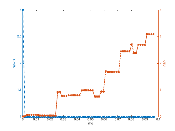
(a) chr18a.

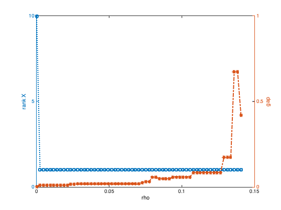
(b) els19.

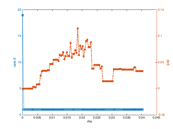
(c) had20.

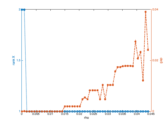
(d) lipa30a.

Figure 1: Effects of paramenters $\rho$ on gaps and ranks of solutions

Although larger $\rho$ can help the solutions satisfying the rank-one constraint in the problem (12) (Proposition 5), the parameter $\rho$ should not be too large. In fact, as demonstrated by (c) had20 and (d) lipa30a in Fig. 1, when $\rho$ increases larger than certain value, the gaps of these two problems oscillate up and down which imply the penalty problem (19) may move away from the target problem (12). In our implementation, a bisection strategy is used for finding a suitable parameter $\rho$ for Algorithm 1.

5.2 Numerical performance

Table 1 summarizes the quality of the solutions obtained by our proposed DCA approach for solving the problems from QAPLIB HAQAPLIB and ‘dre’ instances DreznerHT05 ($107$ instances). It can be seen from Table 1 that for $69$ instances we are able to solve the problems exactly; for $32$ instances we are able to obtain a feasible solution whose gap is less than or equal $4\%$; for $6$ instances we obtain a feasible solution whose gap is larger than $4\%$.

Table 1: Summary of numerical performance of Algorithm 1

Problem set (No.)	gap			Problem
	0	$\leq 4\%$	$>4\%$
drexxx(6)	6	0	0	dre15, dre18, dre21,
				dre24, dre30, dre42
bur26x(8)	0	8	0	bur26a-h
chrxxx(14)	14	0	0	chr12x, chr15x, chr18x,
				chr20x, chr22x, chr25a
els19(1)	1	0	0	els19
escxxx(14)	11	1	2	esc16a-j, esc32a-g
hadxx(5)	5	0	0	had12, had14-had20
kra32x(3)	1	2	0	kra30a-b, kra32
lipaxxx(10)	10	0	0	lipa20x, lipa30x, lipa40x,
				lipa50x, lipa60x
nugxx(13)	8	5	0	nug12, nug14-nug22,
				nug25, nug27, nug28
rouxx(3)	3	0	0	rou12, rou15, rou20
scrxx(3)	3	0	0	scr12, scr15, scr20
skoxx(5)	0	2	3	sko42, sko56, sko64,
				sko72, sko81
ste36x(3)	0	3	0	ste36a-c
taixxx(17)	7	9	1	tai12x, tai15x, tai17x, tai20x,
				tai25x, tai30x, tai35x,
				tai40x, tai50a, tai60b
thoxx(2)	0	2	0	tho30, tho40
Total(107)	69	32	6

The detail numerical results of Algorithm 1 for solving the ‘dre’ instances from DreznerHT05 and QAPLIB HAQAPLIB are reported in Tables LABEL:table2 and LABEL:table3. In the these tables, ‘time’ column (in hours:minutes:seconds) reports the CPU time of Algorithm 1 and ‘permutaion/bound’ column reports the feasible solution generated by solving the relaxation problem (20) of the rank-1 constrained DNN problem (19).

The ‘dre’ problem instances DreznerHT05 are based on a rectangular grid where all nonadjacent nodes have zero weight, making the value of the objective function increase steeply with just a slight change from the optimal permutation. The ‘dre’ instances are difficult to solve, especially for many metaheuristic-based methods, since they are ill-conditioned and hard to break out the ‘basin’ of the local minimal. The best known solutions for the ‘dre’ problems have been found by branch and bound in DreznerHT05 . Notably, by employing our proposed DCA based approach Algorithm 1, we are able to obtain the global optimal solutions of the ‘dre’ problems quite efficiently. For instance, we are able to solve the instance ‘dre42’ by Algorithm 1 exactly in $13$ minutes.

Table 2: Numerical performance of the ‘dre’ problem instances DreznerHT05

Problem	opt	PDCA	gap ($\%$)	time	permutation$/$bound
dre15	306	306	0	11	1 13 4 6 7 9 11 5 12 14 1 15 10 2 3 8
dre18	332	332	0	16	4 14 18 9 10 12 2 15 7 3 5 8 6 11 13 17
					1 16
dre21	356	356	0	33	5 8 17 18 12 13 1 11 3 9 16 4 6 20 7 19
					14 10 15 2 21
dre24	396	396	0	15	3 23 14 21 22 10 16 9 7 5 8 18 13 4 2 17
					1 19 12 11 15 24 6 20
dre30	508	508	0	1:22	28 2 1 17 6 3 11 21 19 22 24 8 26 20 23 13
					4 29 18 25 10 30 16 15 14 12 7 5 27 9
dre42	764	764	0	13:00	3 36 41 28 30 14 34 32 42 37 33 10 27 12 35 9
					7 21 5 29 18 11 8 38 24 2 15 22 6 1 13 19
					40 23 25 39 31 16 17 26 4 20

In Table LABEL:table3, the upper bounds generated by Algorithm 1 are compared with the state of the art optimal values (or the best known upper bounds) in QAPLIB. Except bur$xxx$ and sko$xx$ cases, we find that most instances can either be solved exactly or achieve an upper bound which is accurate up to a relative error of $5\%$ through the penalized DC relaxation. Because the subproblems of the corresponding penalized DC problems are failed to achieve the stopping criteria $10^{-6}$ of SDPNAL+, Algorithm 1 only provides the feasible solutions for bur$xxx$ cases. We note that the QAPLIB bounds were typically achieved using a rather large collection of different algorithms, which generally involve a branch and bound procedure requiring multiple convex relaxations, while our results are achieved by using a single relaxation.

6 Conclusion

This paper established an exact rank constrained DNN formulation of QAP. Under the framework of DC programming, we are able to solve the penalized DC problem efficiently by the semi-proximal augmented Lagrangian method. If the subproblems can be solved successfully, our algorithm usually reaches the optimal solutions of QAP exactly. Even if the subproblem is difficult to solve, our proposed algorithm still can provide a good feasible solution close to the optimal upper bound in QAPLIB. As a future work, we will investigate the structure of the constraints of the penalized DC problem and try to reduce the number of constraints for solving the rank constrained DNN formulation of QAPs more efficiently.

- (1) An, L.T.H., Tao, P.D.: DC programming and DCA: thirty years of developments, Mathematical Programming 169, 5-68 (2018)
- (2) An, L.T.H., Tao, P.D., Huynh, V.N.: Exact penalty and error bounds in DC programming, Journal of Global Optimization 52, 509-535 (2012)
- (3) Anstreicher, K.: Recent advances in the solution of quadratic assignment problems, Mathematical Programming 97, 27-42 (2003)
- (4) Anstreicher, K., Wolkowicz, H.: On Lagrangian relaxation of quadratic matrix constraints, SIAM Journal on Matrix Analysis and Applications 22, 41-55 (2000)
- (5) Attouch, H., Bolte, J.: On the convergence of the proximal algorithm for nonsmooth functions involving analytic features, Mathematical Programming, 116, 5-16 (2009).
- (6) Bi, S.J., Pan, S.H.: Error bounds for rank constrained optimization problems and applications, Operations Research Letters 44, 336-341 (2016)
- (7) Bolte, J., Daniilidis, A., Lewis, A.S.: The Łojasiewicz inequality for nonsmooth subanalytic functions with applications to subgradient dynamical systems. SIAM Journal on Optimization 17, 1205-1223 (2007)
- (8) Bolte, J., Daniilidis, A., Lewis, A.S., Shiota, M.: Clarke subgradients of stratifiable functions. SIAM Journal on Optimization 18, 556-572 (2007).
- (9) Bolte, J., Pauwels, E.: Majorization-minimization procedures and convergence of SQP methods for semi-algebraic and tame programs, Mathematics of Operations Research, 41, 442-465 (2016).
- (10) Bolte, J., Sabach, S., Teboulle, M.: Proximal alternating linearized minimization for nonconvex and nonsmooth problems, Mathematical Programming, 146, 459-494 (2014).
- (11) Burer, S.: On the copositive representation of binary and continuous nonconvex quadratic programs, Mathematical Programming 120, 479-495 (2009)
- (12) Burkard, P.: Quadratic assignment problems, in Handbook of Combinatorial Optimization, Pardalos, P.M., Du, D.Z., Graham, R.L. (ed.), 2741-2814, Springer, New York (2013)
- (13) Buss, F., Frandsen, G. S., Shallit, J.O.: The computational complexity of some problems of linear algebra, Journal of Computer and System Sciences 58, 572-596 (1999)
- (14) Drezner, Z.: The quadratic assignment problem, Location Science, 345-363, Springer, New York (2015)
- (15) Drezner, Z., Hahn, P., Taillard, É.D.: Recent advances for the quadratic assignment problem with special emphasis on instances that are difficult for meta-heuristic methods, Operation Research 139, 65-94 (2005)
- (16) Fu, T., Ge, D., Ye, Y.: On doubly positive semidefinite programming relaxations, Journal of Computational Mathematics 36, 391-403 (2018)
- (17) Gao, Y.: Structured Low Rank Matrix Optimization Problems: A Penalized Approach, PhD thesis, National University of Singapore (2010)
- (18) Gao, Y., Sun, D.F.: A majorized penalty approach for calibrating rank constrained correlation matrix problems, Preprint available at http://www.mypolyuweb.hk/~dfsun/MajorPen_May5.pdf (2010)
- (19) Hahn, P., Anjos, M.: QAPLIB - a quadratic assignment problem library, http://www.seas.upenn.edu/qaplib.
- (20) Horn, R.A., Johnson, C.R.: Matrix Analysis, Cambridge Univeristy Press, New York (1985)
- (21) Kim, S., Kojima, M., Toh, K.C.: A Lagrangian-DNN relaxation: a fast method for computing tight lower bounds for a class of quadratic optimization problems, Mathematical Programming 156, 161-187 (2016)
- (22) Koopmans, T.C., Beckmann, M.J.: Assignment problems and the location of economics activities, Econometrica 25, 53-76 (1957)
- (23) Li, Q., Qi, H.-D.: A Sequential Semismooth Newton Method for the Nearest Low-rank Correlation Matrix Problem. SIAM Journal on Optimization 21, 1641-1666 (2011).
- (24) Lin, C.-J., Saigal, R.: On solving large-scale semidefinite programming problems a case study of quadratic assignment problem. Technical report, Department of Industrial and Operations Engineering, University of Michigan, Ann Arbor MI, (1997)
- (25) Liu, T., Pong, T.K., Takeda, A.: A refined convergence analysis of with applications to simultaneous sparse recovery and outlier detection. Computational Optimization Applications 73, 69-100 (2019).
- (26) Motzkin, T.S., Straus, E.G.: Maxima for graphs and a new proof of a theorem of Turan, Canadian Journal of Mathematics 17, 533-540 (1965)
- (27) Murty, K.G., Kabadi, S.N.: Some NP-complete problems in quadratic and nonlinear programming, Mathematical Programming 39, 117-129 (1987)
- (28) Povh, J., Rendl, F.: A copositive programming approach to graph partitioning, SIAM Journal on Optimization 18, 223-241 (2007)
- (29) Povh, J., Rendl, F.: Copositive and semidefinite relaxations of the quadratic assignment problem, Discrete Optimization 6, 231-241 (2009)
- (30) Ramana, M., Tunçel, L., Wolkowicz, H.: Strong duality for semidefinite programming, SIAM Journal on Optimization 7, 641-662 (1997)
- (31) Rendl, F., Sotirov, R.: Bounds for the quadratic assignment problem using the bundle method, Mathematical Programming 109, 505-524 (2007)
- (32) Rockafellar, R.T.: Convex Analyis, Princeton University Press, Princeton (1970)
- (33) Rockafellar, R.T.: Conjugate Duality and Optimization. SIAM (1974).
- (34) Sahni, S., Gonzalez, T.: P-complete approximation problems, Journal of the ACM 23, 555-565 (1976)
- (35) Sun, D.F., Toh, K.C., Yuan, Y.C., Zhao, X.Y.: SDPNAL+: A Matlab software for semidefinite programming with bound constraints (version 1.0), Optimization Methods and Software, in print (2019)
- (36) Todd, M.J.: Semidefinite optimization. Acta Numerica. 10, 515-560 (2001).
- (37) Vandenberghe, L., Boyd, S.: Semidefinite programming, SIAM Review 38, 49-75 (1996)
- (38) Wen, Z.W., Goldfarb, D., Yin, W.T.: Alternating direction augmented Lagrangian methods for semidefinite programming, Mathematical Programming Computation 2, 203-230 (2010)
- (39) Weyl, H.: Das asymptotische verteilungsgesetz der eigenwerte linearer partieller differentialgleichungen (mit einer anwendung auf die theorie der hohlraumstrahlung, Mathematische Annalen 71, 441-479 (1912)
- (40) Yang, L.Q., Sun, D.F., Toh, K.C.: SDPNAL+: A majorized semismooth Newton-CG augmented lagrangian method for semidefinite programming with nonnegative constraints, Mathematical Programming Computation 7, 331-366 (2015)
- (41) Yoshise, A., Matsukawa, Y.: On optimization over the doubly nonnegative cone, Proceedings of 2010 IEEE Multi-conference on Systems and Control, 13-19 (2010)
- (42) Zhao, Q., Karisch, S.E., Rendl, F., Wolkowicz, H.: Semidefinite programming relaxations for the quadratic assignment problem, Journal of Combinatorial Optimization 2, 71-109 (1998)
- (43) Zhao, X.Y., Sun, D.F., Toh, K.C.: A Newton-CG augmented lagrangian method for semidefinite programming, SIAM Journal on Optimization 20, 1737-1765 (2010)