Homogeneously derived transit timings for 17 exoplanets and reassessed TTV trends for WASP-12 and WASP-4

Abstract

We homogeneously analyse $\sim 3.2\times 10^{5}$ photometric measurements for $\sim 1100$ transit lightcurves belonging to $17$ exoplanet hosts. The photometric data cover $16$ years 2004–2019 and include amateur and professional observations. Old archival lightcurves were reprocessed using up-to-date exoplanetary parameters and empirically debiased limb-darkening models. We also derive self-consistent transit and radial-velocity fits for $13$ targets. We confirm the nonlinear TTV trend in the WASP-12 data at a high significance, and with a consistent magnitude. However, Doppler data reveal hints of a radial acceleration about $(-7.5\pm 2.2)$ m/s/yr, indicating the presence of unseen distant companions, and suggesting that roughly $10$ per cent of the observed TTV was induced via the light-travel (or Roemer) effect. For WASP-4, a similar TTV trend suspected after the recent TESS observations appears controversial and model-dependent. It is not supported by our homogeneus TTV sample, including $10$ ground-based EXPANSION lightcurves obtained in 2018 simultaneously with TESS. Even if the TTV trend itself does exist in WASP-4, its magnitude and tidal nature are uncertain. Doppler data cannot entirely rule out the Roemer effect induced by possible distant companions.

Authors’ affiliations

¹Saint Petersburg State University, Faculty of Mathematics & Mechanics, Universitetskij pr. 28, Petrodvorets, St Petersburg 198504, Russia
²Central Astronomical Observatory at Pulkovo of Russian Academy of Sciences, Pulkovskoje sh. 65/1, St Petersburg 196140, Russia
³University of Hertfordshire, Centre for Astrophysics Research, STRI, College Lane, Hatfield AL10 9AB, UK
⁴Geneva Observatory, University of Geneva, Chemin des Mailettes 51, 1290 Versoix, Switzerland
⁵Acton Sky Portal (Private Observatory), Acton, MA, USA
⁶Instituto de Astronomía Teoríca y Experimental, Universidad Nacional de Córdoba, Laprida 854, Córdoba X5000BGR, Argentina
⁷School of Physics, Trinity College Dublin, The University of Dublin, Dublin 2, Ireland
⁸Facultad de Ciencias Astronómicas y Geofísicas - Universidad Nacional de La Plata, Paseo del Bosque S/N - 1900 La Plata,
Argentina
⁹Instituto de Astrofísica de La Plata (CCT La Plata - CONICET/UNLP), Argentina
¹⁰Ankara University, Faculty of Science, Department of Astronomy and Space Science, TR-06100, Tandogan, Ankara, Turkey
¹¹Baronnies Provençales Observatory, Hautes Alpes - Parc Naturel Régional des Baronnies Provençales, F-05150 Moydans, France
¹²Taurus Hill Observatory, Warkauden Kassiopeia ry., Härkämäentie 88, 79480 Kangaslampi, Finland
¹³Physics and Engineering Physics Department, University of Saskatchewan, 116 Science Place, Saskatoon, Saskatchewan,
S7N 5E2, Canada
¹⁴Observatoire de Vaison la Romaine, 1075 RD 51, Le Palis, 84110 Vaison-la-Romaine, France
¹⁵National Youth Space Center, Goheung, Jeollanam-do, 59567, S.Korea
¹⁶Department of Astronomy and Space Science, Chungbuk National University, Cheongju-City, 28644, S.Korea
¹⁷Institute of Theoretical Physics and Astronomy, Vilnius University, Sauletekio al. 3, Vilnius 10257, Lithuania
¹⁸Horten Videregående Skole, Bekkegata 2, 3181 Horten, Norway
¹⁹Ngileah Observatory, 144 Kilkern Road, RD 1. Bulls 4894, New Zealand
²⁰Observatori Astronòmic Albanyà, Camí de Bassegoda s/n, 17733 Albanyà, Spain
²¹Astronomical Observatory, DSFTA - University of Siena, Via Roma 56, 53100 - Siena, Italy
²²El Sauce Observatory, Coquimbo Province, Chile
²³School of Physical Sciences, The Open University, Milton Keynes, MK7 6AA, UK
²⁴La Vara, Valdes Observatory, 33784 Munas de Arriba, Valdes, Asturias, Spain
²⁵Anunaki Observatory, Calle de los Llanos, 28410 Manzanares el Real, Spain
²⁶AAVSO, Private Observatory, Elgin, OR 97827, USA
²⁷Observatory Saint Martin, code k27, Amathay Vesigneux, France
²⁸Green Island Observatory, Code B34, Gecitkale, Famagusta, North Cyprus
²⁹Institute of Solar-Terrestrial Physics (ISTP), Russian Academy of Sciences (Siberian Branch), Irkutsk 664033, p.b. 291,
Lermontov street 126a, Russia
³⁰Institute of Astronomy of Russian Academy of Sciences, Pyatnitskaya Str. 48, Moscow 119017, Russia
³¹Ulugh Beg Astronomical Institute of Uzbek Academy of Sciences, Astronomicheskaya Str. 33, Tashkent 100052, Uzbekistan

1 Introduction

Transit photometry is now one of the primary exoplanets detection tools. This method has a very promising descedant branch — transit timing variations, or TTVs. The outstanding value of the TTV method comes from its ability to directly detect observable hints of $N$-body interactions in a planetary system. This method is even capable of detecting previously unknown planets (Agol & Fabrycky, 2017), and directly reveal tidal interactions with the star, like now famous example of WASP-12 b (Maciejewski et al., 2018b; Bailey & Goodman, 2019). This star demonstrates subtle period drift, as if the planet was spiraling down onto its host star. Such a physical phenomenon brings us unique opportunities to test the theories of tidal planet-star interaction and even to put some constraints on the interior structure of this exoplanet (Patra et al., 2017). Recently, hints of an analogous TTV drift were also reported for WASP-4 (Bouma et al., 2019), based on the first TESS observations.

Our present work is devoted to further development of the TTV method. Basically, it presents results of a revised analysis following (Baluev et al., 2015) but including additional targets, expanded photometric data, and improved processing algorithms. However, if the goal of Baluev et al. (2015) was to demonstrate the potential of amateur observations in the TTV field, the primary accent here is to highlight the importance of using homogeneously derived TTVs.

The exoplanetary transit times published in literature are derived by multiple independent teams that used very different methods and models. For example, some works assume linear limb-darkening law, but some quadratic. The limb-darkening coefficients may be fixed at theoretically predicted values, or fitted as free parameters of the lightcurve. The photometric noise can be modelled differently as well: while some early measurements did not yet take into account the red noise, others did, but all in different ways. Some tried to reduce systematic effects by decorrelating them with airmass, some use more complicated correlation models, and some just fit the systematics by a deterministic model (e.g. trends plus multiple oscillations).

Moreover, any transit lightcurve fit also depends on the exoplanetary parameters (planet/star radii ratio, impact parameter, etc.) which have an obvious tendency to improve their accuracy with time. While many earlier transit observations were rather inaccurate because they could not rely on good exoplanetary parameters, later ones can use a larger record of observations to derive more accurate results.

As such, the transit times published in the literature appear very heterogeneous: they may have subtle systematic biases, including biases in their uncertainties. Those biases are difficult to deal with, because they vary from one team to another in an impredictable manner. Hence, it might appear too difficult to analyse such merged TTV data as if they were homogeneous, ultimately resulting in false detections of spurious variations and so on.

This work presents an attempt to carefully reprocess the archival and new observations in a homogeneous way, relying on the same analysis protocol, including the use of the same methods and of the same transit and noise models. Now we can reprocess the entire photometry set available for each target in a self-consistent manner, i.e. we should not necessarily fit all the transits for the same target independently. This approach was already tested in (Baluev et al., 2015), and it allows us to reduce the number of degrees of freedom of the fit, thus improving the usability of lower-quality observations.

Such a goal naturally implies substantial analysis of the available photometric data, careful identification of possibly outlying measurements or even entire lightcurves. Such a work necessarily implies an investigation of the models involved, in particular the limb-darkening models and noise models. This also includes an analysis of the photometric noise potentially yielding improved data-processing strategies.

Moreover, we now aim to undertake a multimethod study not relying on just the photometric observations. We performed a self-consistent analysis of our homogeneously processed photometry jointly with Doppler data, since the combination of the transit and Doppler methods allows for a much more comprehensive characterization of a planetary system. This is especially important for several unique exoplanets, like the above-mentioned WASP-12 or WASP-4 demonstrating possible TTV trends. In particular, relatively little attention was paid so far to a yet another explanation of such trends, based on the light-travel effect induced by outer bodies (Irwin, 1952).

Finally, this work represents the first big practical test of the EXPANSION project (EXoPlanetary trANsit Search with an International Observational Network), grown on the basis of the ETD (Exoplanet Transit Database) that was used by Baluev et al. (2015). Now EXPANSION is a standalone international project joining a network of several dozens of relatively small-aperture telescopes, aimed to monitor the exoplanetary transits (Sokov et al., 2018). This network covers amateur as well as professional observatories spreaded over the world in the both hemispheres.

The structure of the paper is as follows. In Sect. 2 we provide a detailed description of the data that we analyse. In Sect. 3 we introduce the algorithms used to process the photometric data. In Sect. 4 we present results of empirical debiasing of the limb-darkening theoretic models. In Sect. 5 we present the TTV data derived for our $17$ targets and results of their analysis, including a detailed discussion of possible TTV trends in WASP-12 and WASP-4. In Sect. 6 we present results of self-cosistent fits using both the transit and radial velocity data, available for $13$ targets. In Sect. 7 we discuss in yet more detail the case of WASP-12, deriving a purely tidal part in its observed TTV trend.

2 Photometric and Doppler data

The EXPANSION project performs a long-term monitoring of exoplanetary transits. Amateur and professional observatories from Russia, Europe, North and South Americas with relatively small telescopes from 25 cm to 2 m are used in the photometric observations (Sokov et al., 2018). We used data from this network, including all the data from ETD that were used in (Baluev et al., 2015). Additionally, we used lightcurves published in the literature or kindly provided by the observers, as listed in Table 1. Most of them are available in the VIZIER database.

We expanded our targets list by seven exoplanets: Qatar-2, WASP-3, -6, -12, HAT-P-3, -13, and XO-5, thus increasing their number to $17$. The total amount of the input data has grown considerably. This time we had $\sim 3\times 10^{5}$ photometric measurements in $\sim 1000$ lightcurves, compared to $\sim 8\times 10^{4}$ measurements in $\sim 300$ lightcurves processed by Baluev et al. (2015).

Whenever necessary, the timestamps in the photometric series were transformed to the ${\rm BJD}_{\rm TDB}$ system by means of the public IDL software developed by Eastman et al. (2010). To perform this reduction, we used ICRS coordinates through the SIMBAD database which originate from GAIA DR2 (Brown et al., 2018). We did not apply any correction to these coordinates due to proper motion, since this would imply only a negligible correction to the time (below $\sim 0.1$ sec).

Table 1: Sources of the photometric data (not including the EXPANSION project).

Target	References	Note
CoRoT-2	Gillon et al. (2010)
GJ 436	Gillon et al. (2007)
	Bean et al. (2008)	HST Fine Guidance Sensor
	Shporer et al. (2009)
	Cáceres et al. (2009)	Very high cadence; we binned these data to $10$ sec chunks
HAT-P-3	Torres (2007)
	Chan et al. (2011)
	Nascimbeni et al. (2011a)	Data initially uploaded to VIZIER were not actually in BJD system as claimed (priv. comm.); correct data uploaded in 2017
	Mancini et al. (2018)
HAT-P-13	Bakos et al. (2009)
	Szabó et al. (2010)
	Nascimbeni et al. (2011b)
	Fulton et al. (2011)
	Southworth et al. (2012)
HD 189733	Bakos et al. (2006)
	Winn et al. (2007a)	T10APT data involve double HJD correction by mistake (priv. comm.)
	Pont et al. (2007)	HST Advanced Camera for Surveys
	McCullough et al. (2014)	HST Wide Field Camera 3
	Kasper et al. (2019)	Multi-band transmission spectroscopy; very high accuracy data
Kelt-1	Siverd et al. (2012)
	Maciejewski et al. (2018b)
Qatar-2	Bryan et al. (2012)	It is not fully clear, whether the “BJD” times are given in UTC or TDB system. We assume BJD TDB, because the TTV residuals look bad otherwise.
	Mancini et al. (2014)
TrES-1	Winn et al. (2007b)
WASP-2	Southworth et al. (2010)	Danish telescope timings might be unreliable (Nikolov et al., 2012; Petrucci et al., 2013)
WASP-3	Tripathi et al. (2010)
	Nascimbeni et al. (2013)
WASP-4	Wilson et al. (2008)
	Gillon et al. (2009a)
	Winn et al. (2009)	Superseded by Sanchis-Ojeda et al. (2011)
	Southworth et al. (2009b)	Danish telescope timings might be unreliable (Nikolov et al., 2012; Petrucci et al., 2013)
	Sanchis-Ojeda et al. (2011)
	Nikolov et al. (2012)
	Petrucci et al. (2013)	These data were kindly provided by the authors
WASP-5	Southworth et al. (2009a)	Danish telescope timings might be unreliable (Nikolov et al., 2012; Petrucci et al., 2013)
WASP-6	Gillon et al. (2009b)
	Tregloan-Reed et al. (2015)
WASP-12	Hebb et al. (2009)	These data were kindly provided by the authors
	Chan et al. (2011)
	Maciejewski et al. (2013)	Partly superseded by Maciejewski et al. (2016)
	Stevenson et al. (2014)	Multi-band transmission spectroscopy; very high accuracy data
	Maciejewski et al. (2016)
	Maciejewski et al. (2018b)
WASP-52	Chen et al. (2017)	Multi-band transmission spectroscopy; very high accuracy data
	Mancini et al. (2017)
XO-2N	Fernandez et al. (2009)
	Kundurthy et al. (2013)
	Damasso et al. (2015)
XO-5	None

Additionally, we used the precision radial velocity (RV) measurements obtained from the archival spectra of the HARPS, HARPS-N, SOPHIE, and HIRES spectrographs. This involves the following targets from our photometry sample: Corot-2, GJ 436, TrES-1, WASP-2, -4, -5, -6, -12, HD 189733, XO-2N. The spectra were processed with the HARPS–TERRA pipeline (Anglada-Escudé & Butler, 2012). Some of these data represent reprocessed versions of the RV data available in the literature, e.g. from (Baluev et al., 2015), and some are new. Whenever performing a self-consistent transit and radial velocity analysis we transform all the Doppler time stamps to the ${\rm BJD}_{\rm TDB}$ system consistent with the photometry. However, the RV data that we release here correspond to the UTC rather than TDB system (as traditionally adopted for this type of the data).

Since Wilson et al. (2008), additional $31$ RV measurements have been obtained for WASP-4 with the high resolution spectrograph CORALIE on the Swiss $1.2$ m Euler telescope at La Silla Observatory, Chilie (Queloz et al., 2001). RVs were re-computed for the new data and the dataset presented in Wilson et al. (2008), for $45$ measurements in total, by cross-correlating each spectrum with a G2 binary mask, using the standard CORALIE data-reduction pipeline.

For WASP-2, WASP-3, WASP-4, WASP-12, and XO-5 additional HIRES observations were presented by Knutson et al. (2014), which we included in the analysis in the published form. The Keck RV data from (Knutson et al., 2014) for XO-2N and GJ 436, and from (Albrecht et al., 2012) for GJ 436 were not used as they were found in our TERRA-processed sample. The HAT-P-13 data available in (Knutson et al., 2014) mysteriously appeared older and much less complete than RV data set by Winn et al. (2010), so we used the latter one. Some more in-transit RV data for WASP-12 are also mentioned in (Albrecht et al., 2012) but not published.

The data files containing the photometric and radial-velocity measurements are attached as the online-only material. The format of the files follows that of (Baluev et al., 2015). Concerning the RVs, we currently release only a partial set, since we still plan to seek more RV data and perform their more detailed analysis in a future work.

We notice that some TERRA-processed RV data in (Baluev et al., 2015) appeared partly erratic. First, the HARPSN data for HD 189733 appeared entirely wrong because they belong to its known companion B. Secondly, the difference between the new and old HARPS data for GJ 436 revealed a clear systematic trend indicating some processing error in the old data set. The long-term trend was highly significant in the previous RV release, but now it disappeared.

3 Deriving transit times from photometry

Our derivation of transit timing variations from photometry uses a similar procedure to that of Baluev et al. (2015) which we updated to follow the processing stages below.

1. Fit the raw transit photometry and the resulting resulting transit timings with a reference TTV model (linear ephemeris plus a possible quadratic trend, see eq. (5)).

2. Clean TTV outliers (bad lightcurves) by verifying the TTV residuals and then reprocessing the remaining data.

3. Clean photometry outliers in the remaining lightcurves in a similar way and then reprocess the data.

4. Reprocess the data using semi-empirical limb-darkening coefficients for lightcurves in which the limb-darkening was ill-fitted or had poor accuracy. The semi-empirical values are based on Claret & Bloemen (2011) corrected for the systematic biases derived in Sect. 4.

5. Among the remaining lightcurves, identify higher-quality (HQ) ones, and reprocess them separately.

We note that in our previous work we were only able to follow Stages 1 and 3. Stage 2 could not be completed due to a relative lack of TTV data. Stage 4 was not performed due to a simplistic limb-darkening treatment, which is now revised, and Stage 5 was absent. Most of the analysis was performed using the PlanetPack software (Baluev, 2013, 2018). We now consider each stage in more detail.

3.1 Stage 1: lightcurve fitting

The light curve fitting is based on maximum-likelihood fitting with a dedicated model of the photometric noise and follows (Baluev et al., 2015). As in that work, we use circular model of the curved transiter orbital motion. Most of our targets do not have a detectable orbital eccentricity, except for GJ436b. However, the photometric data for GJ436 appeared mostly of a too low quality. Except for a very few space-based HST observations, they do not justify the use of a general Keplerian model. In any case, we include non-zero orbital eccentricities in the joint transit+Doppler analysis below.

The initial steps of the algorithm involve a set of preliminary fits, needed to avoid pathological solutions and fitting traps:

1. Fit the data with a fixed transit impact parameter, fixed limb darkening coefficients and with a strictly quadratic TTV ephemeris. Contrary to (Baluev et al., 2015), who adopted a linear TTV ephemeris, here we decided to use a quadratic one because now we have at least two candidates with a quadratic TTV trend (WASP-12 and WASP-4), and all other targets should be processed homogeneously.

2. Refit after releasing the transit impact parameter and mid-times.

3. Refit after releasing limb darkening coefficients (except for those that are fixed at the corrected theoretical values at Stage 4 or 5).

4. Determine very high-quality lightcurves that allow independent fitting of the limb darkening coefficients and if such lightcurves exist, refit the model yet again.

After these initial stages, our red noise auto-detection sequence follows that of Baluev et al. 2015; Baluev 2018. Our criteria for a robust red noise detection were: (i) the log-likelihood ratio statistic $Z$ should be at least $2$, implying the asymptotic false detection probability $\chi^{2}_{2}(Z)=\exp(-Z)\sim 14$ per cent, (ii) the uncertainty in the red jitter $\sigma_{\rm r}$ is at most the estimated value (iii) the uncertainty in the red noise timescale $\tau$ is at most twice the estimated value. These criteria appear very mild (even more mild than in Baluev et al. 2015). In fact, they assume that most of the lightcurves must contain some red noise by default, except for the cases whenever the red noise could not be modelled reliably.

In this work we used $3$ starting initial values for $\tau$, thus running up to $3$ probe red-noise fits for each lightcurve. These initial values were spreaded logarithmically in the range from $T/N$ to $T$ (where $T$ is the total time span of the lightcurve, and $N$ is the number of its photometric measurements). In (Baluev et al., 2015) just a single initial value $\tau=T/\sqrt{N}$ was used, with a single probe fit per a lightcurve. It appeared that among our $\sim 1000$ lightcurves, almost all reveal their red noise after just this very first trial fit. However, in a few cases it appeared that the first fit did not converge to a robust solution because the actual best fitting value of $\tau$ was too far from $T/\sqrt{N}$. By adding two more probe fits starting from $\tau$ closer to the low and upper limits of the range, we could robustly detect the red noise in several lightcurves additionally.

But even with these very mild detection criteria and multiple trial fits it appeared that only $1/4$ to $1/3$ of our lightcurves (depending on the target) revealed an individually fittable red noise. This is in agreement with Baluev et al. (2015), however such a low fraction of the red-noised lightcurves still appears surprising. The red noise may exist in the rest of lightcurves too, but with ill-fitted individual parameters. Therefore, leaving the noise models in such a partial model-mixed state might make the resulting TTV data less homogeneous. For example, the uncertainties in the white-noise portion of TTV data may appear systematically smaller than in the red-noise one. To soften this effect we tried to fit the red noise in the remaining lightcurves in an averaged sense. Since the most uncertain and poorly determinable red noise parameter is $\tau$, we assumed that this $\tau$ is the same among all the lightcurves that did not reveal an individually detectable red noise. While binding $\tau$ at such a shared ‘average’ value, the value of $\sigma_{\rm r}$ was still assumed individually fittable for each lightcurve to allow an adaptive match of the red noise magnitude. In this way, if this derived shared $\tau$ appeared inconsistent with the actual observations in a given lightcurve then this $\tau$ could be just ignored by reducing $\sigma_{\rm r}$ to zero.

After that the fraction of lightcurves enclosed by a red-noise model was raised to $50-80$ per cent, depending on the target. The rest of the data had the best fitting $\sigma_{\rm r}=0$, implying that they contradict either the derived shared $\tau$, or the red-noise hypothesis itself. This might formally suggest the presence of a blue noise instead (or $\sigma_{\rm r}^{2}<0$). If the red noise infers an increase of the TTV uncertainties, the blue noise would reduce them below the level expected from the white noise. Such an apparent effect may appear due to starspot transit events (see below), but they might also imply large individual timing biases which we do not detect or reduce in this work. In such circumstances, we do not allow the TTV uncertainties to decrease below their white-noise estimations.

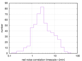
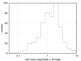
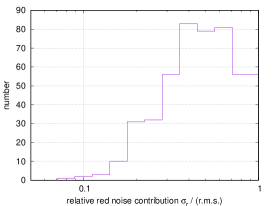
Figure 1: Histograms of the estimated photometric red noise parameters, $\tau$ and $\sigma_{\rm r}$, and of the relative red noise contribution in the total RMS. We used only those estimations of $\tau$ and $\sigma_{\rm r}$ on Stage 4 that exceeded their respective uncertainty.

Since we have a large set of red noise estimations for numerous lighcurves, it is now possible to consider some statistics. In Fig. 1 we show the histograms of the derived red noise parameters $\tau$ and $\sigma_{\rm r}$, and of the ratio $\sigma_{\rm r}/$(RMS), the relative red noise contribution in the total error budget. We can see that $\tau$ spans a wide range from $\sim 10$ sec to $\sim 50$ min, but is primarily located in the range $1-5$ min. The typical magnitude of the red noise is $\sim 1$ mmag, but also can deviate a lot from this peak value. The relative red noise contribution is typically above $30$ per cent (smaller values typically cannot be detected or estimated reliably, so they are mostly ignored in these histograms).

Yet another major difference from (Baluev et al., 2015) is a more careful treatment of the limb darkening. As before, we adopted a quadratic limb darkening model:

$$I(\rho)/I(0)=1-A(1-\mu)-B(1-\mu)^{2},\quad\mu=\sqrt{1-\rho^{2}},$$ (1)

where $\rho$ is the projected distance from the disk center, and coefficients $A$ and $B$ should satisfy the constraints

$$A+B\leq 1,\quad A+2B\geq 0,\quad A\geq 0,$$ (2)

which guarantee that $I(\rho)$ never turns negative and always remains monotonically decreasing (no limb brightening allowed), see Baluev et al. 2015; Kipping 2013.

In (Baluev et al., 2015) the limb darkening coefficients $A$ and $B$ were assumed the same for the most of the lightcurves, regardless of the spectral band. But now we considered this as an inadmissibly rough assumption. Although a fully independent fit of these coefficients for every lightcurve is unnecessary (and even practically impossible), we need at least to fit them independently for different spectral filters.

We split all available lightcurves into several sets that correspond to the same or similar spectral bands. For example, we combined in a single set the Johnson $R_{J}$ and Cousins $R_{C}$ filters, as well as the Sloan $r$ or $r^{\prime}$ ones, treating them all as the same “generic $R$” filter. The theoretically predicted limb darkening coefficients appear almost equal in all these filters: the differences are smaller than e.g. those implied by different models of stellar atmosphere in (Claret, 2000, 2004; Claret & Bloemen, 2011). Thus we sorted all our data into 8 classes, corresponding to the following “generic” spectral ranges: $U$, $B$, $V$, $G$, $R$, $I$, $Z$, $K$. Many lightcurves (mostly amateur ones) were obtained without any filter at all, or using a wide-band IR-UV cut-off filter, and we joined all such data under another class labelled “clear”.

A few lightcurves could not be assigned to any of the above band classes, because they were obtained in another spectral band or with a different technique. Most of that data appeared of an exceptional quality, so we always fit their limb darkening coefficients independently. These special cases include observations from Hubble Space Telescope, “white” lightcurves from transmission spectroscopy, and data from some other specialized instruments.

Finally, we carried out a systematic comparison of the resulting “observed” coefficients $A$ and $B$ with their theoretically predicted values based on (Claret, 2000, 2004; Claret & Bloemen, 2011). This comparison revealed certain systematic biases, discussed in Section 4 below.

3.2 Stages 2 and 3: cleaning the outliers

The cleaning of outliers is performed as in (Baluev et al., 2015), by means of inspecting the Gaussian quantile-quantile (QQ) plots of the TTV residuals. The QQ plot is a non-linearly re-scaled graph of the empirical cumulative distribution $F_{\rm emp}(\varepsilon)$ of the normalized residuals $\varepsilon_{i}=r_{i}/\sigma_{i}$, where $r_{i}$ is the best-fit residual and $\sigma_{i}$ is the modelled standard deviation. If the input data were good and all models correct, then this $F_{\rm emp}(\varepsilon)$ should be close to standard Gaussian, $F(\varepsilon)=\Phi(\varepsilon)$. Hence the quantile function $Q(\varepsilon)=\Phi^{-1}(F_{\rm emp}(\varepsilon))$ should be close to $Q(\varepsilon)=\varepsilon$.

The graph of $Q(\varepsilon)$ is the QQ plot that we examine. These plots are given in the online-only Fig. 2, 1st row. We can see that the empirical curves are indeed close to the main diagonal, suggesting mostly Gaussian noise, but a number of outliers deviate in the tails much more than a normal distribution would allow. Therefore, the outliers can be identified as points that reside in these tails. The photometric outliers are detected in the same way as TTV ones. The corresponding QQ plots are shown in the online-only Fig. 2, 2nd row.

We reviewed the list of potential $\sim 20$ TTV outliers, and decided to manually ‘whitelist’ two lightcurves looking like outliers. Namely, this is one lightcurve for HAT-P-13 from (Szabó et al., 2010) and one for HD 189733 from (Kasper et al., 2019), both with $\varepsilon\simeq 4$. Concerning HAT-P-13, it demonstrated inconclusive hints of a TTV in the past, and it might appear to be the case that (Szabó et al., 2010) measurements actually reveal a true TTV, rather than a statistical outlier (e.g. induced by known non-transiting companions, see Winn et al. 2010). However, after that we noticed that this large normalized residual was finally reduced on Stage 4, thanks to using corrected limb-darkening coefficients which appeared ill-fit on Stage 3. Concerning the HD 189733 lightcurve by Kasper et al. (2019), it belongs to a homogeneous set of high-quality transmission spectroscopy observations. The other observations also have rather large $\epsilon$ level. We decided to allow all the Kasper et al. (2019) data to Stage 5 despite the particular lightcurve being rather anomalous. Possible reasons of such anomalies in the Kasper et al. (2019) data are discussed in Sect. 5.1.

3.3 Stage 4: applying empirically corrected limb-darkening

Many lightcurves have relatively poor quality, so it is not possible to reliably fit a two-parametric limb-darkening law (1). Therefore, on Stage 3 multiple estimates appear to have large uncertainties in $A$ and $B$ about unity, or the coefficients themselves lie on the boundary of their admissible domain (Kipping, 2013), indicating a poor fit. To overcome these issues, we performed one more processing pass, fixing the limb-darkening coefficients with poor accuracy at certain semi-empirical values. See more detailed discussion and motivation in Sect. 4.

3.4 Stage 5: determining high quality lightcurves

To identify transit times of a higher quality, we first introduce the “quality characteristic” of a lightcurve:

$$\mathcal{Q}=\frac{\sqrt{\text{measurements density}}}{\text{residuals RMS}}$$ (3)

The quantity $1/\mathcal{Q}$ determines the uncertainty offered by a “standard” chunk of the lightcurve of a unit length. The uncertainty of an arbitrary chunk of length $t$ scales as $1/(\mathcal{Q}\sqrt{t})$. Here we neglect possible red noise, so even neighboring measurements are assumed uncorrelated.

This characteristic is not yet indicative concerning a particular exoplanet. Let $\tau$ be the transit duration, and $r^{\prime}=r_{\rm pl}/R_{\star}$ be the planet/star radii ratio. Then the uncertainty of the in-transit piece of the lightcurve would be $1/(\mathcal{Q}\sqrt{\tau})$, and it should be compared to the transit depth $r^{\prime 2}$. That is, the following normalized parameter:

$$\mathcal{Q}^{\prime}=\mathcal{Q}\sqrt{\tau}/r^{\prime 2}$$ (4)

can serve as our idealized quality characteristic. Say, $\mathcal{Q}^{\prime}=100$, then the transit depth can be measured with an accuracy of $1$ per cent, while $\mathcal{Q}^{\prime}=10$ implies relative accuracy of $10$ per cent.

Now let us plot the empirical distribution of $\mathcal{Q}^{\prime}$ computed for all our lightcurves (online-only Fig. 2, bottom row). We can see that $\mathcal{Q}^{\prime}$ varies in an very wide range from a few tens to a few thousands. We choose a threshold $Q^{\prime}>100$ to select the HQ lightcurves. Such a threshold keeps about $2/3$ of the entire sample, so it is a relatively mild filter. Our goal was mainly to filter out only very inaccurate and probably useless data, rather than to select a minor portion of highly accurate ones.

Note that whenever a lightcurve has low $\mathcal{Q}^{\prime}$, this does not necessarily mean that it must be immediately removed from the analysis as unreliable. Such a lightcurve just has a poor overall accuracy, but it already survived the normality tests of the previous processing stages. Statistically, the derived timing value remains quite admissible and usable (within its uncertainty). Below we consider results of Stage 4 and Stage 5 simultaneously so the reader can compare them.

4 Empirical calibration of the limb-darkening coefficients

Using the technique presented above, we performed a per-target and per-band fit of the limb darkening coefficients $A$ and $B$ in the quadratic model (1). After that, we compared these empirical estimates with their theoretically predicted values from (Claret, 2000, 2004) and their update from (Claret & Bloemen, 2011) band-by-band. The coefficients for the “clear” band-class were compared with the bolometric estimates by Claret. We utilized the jktld code by Southworth (2015) that offers a convenient interface for interpolating the original tables by Claret. The necessary stellar parameters ($T_{\rm eff}$, $\log g$, [Fe/H]) were taken mainly from the SWEET-Cat (Santos et al., 2013), and from (Siverd et al., 2012) for Kelt-1. In almost all cases we used the coefficients corresponding to the ATLAS models, except for GJ 436, for which only the PHOENIX-based coefficients were available. We assumed microturbulence velocity $v_{t}$ of $2$ km/s for all cases.

We found that many of our $A$ and $B$ estimations, even the most accurate ones, significantly deviate from theoretical values. In itself, this is not very surprising, because the theoretical values are expected to have some biases (Heyrovský, 2007). Even if the theoretical brightness profile was entirely perfect, the two-parameter models such as (1) cannot approximate it everywhere equally well. The resulting “theoretical” coefficients $A$ and $B$ depend on how we fit this profile: they may appear biased to better fit one its portion or another. And they should not necessarily coincide with the empirical values obtained from transit fitting (even if the latter had no significant errors at all).

In online-only Fig. 3, some worst-case discrepancies are demonstrated. The empirical $A$ and $B$ estimations correspond to the processing Stage 3, while the theoretical values were derived from (Claret, 2000, 2004), and one can see that they systematically deviate by $\sim 0.1-0.2$.

Then we computed the universal shifts $\Delta A$ and $\Delta B$, necessary to minimize the differences between the observed and theoretical coefficients. The weighted least squares fit yielded the biases $\Delta A=0.059\pm 0.008$ and $\Delta B=-0.172\pm 0.014$ for the quadratic law, and $\Delta A=-0.112\pm 0.002$ for the linear law. These shifts refer to the older tables by Claret (2000, 2004), ATLAS models, and take into account only the UBVGRIZK filters.

By fitting the newer models by Claret & Bloemen (2011), corresponding to the flux-conservation method (FCM), and for the same spectral filters as above, we obtained the following biases: $\Delta A=0.004\pm 0.008$ and $\Delta B=-0.099\pm 0.014$ for the quadratic law, and $\Delta A=-0.035\pm 0.002$ for the linear law. The newer tables are clearly better, though some minor bias still remains in $B$. By adding the latter best-fitting corrections to the theoretical $A$ and $B$ values the agreement can be improved remarkably. This becomes obvious in several high-accuracy cases (e.g. WASP-4, Qatar-2), see online-only Fig. 4.

The coefficients from Claret & Bloemen (2011) obtained by least-square fit of the brightness profile appear less accurate than the FCM ones and more similar to those from (Claret, 2000, 2004). The differences between various systems of the limb-darkening coefficients highlight the need for a homogeneous TTV analysis, based on simultaneous fitting of all raw lightcurves at once and using the same analysis pipeline. Direct mixing of independently derived timing measurements, especially those released before or after the 2011 update, may lead to spurious timing biases.

In this work, we adopt a hybrid approach to model the limb-darkening profile following the key aspects below.

1. If at Stage 3 both $A$ and $B$ had a fitting uncertainty of better than $0.2$ and simultaneously did not reside on either boundary of (2) then we did not rely on the theoretical values. Even the corrected ones may still appear to be biased for an individual star, so we allowed these coefficients to be fitted from the transit curves as free parameters (still taking into account the common binding constraints per each spectral band class).

2. The limb-darkening coefficients corresponding to filters other than UBVGRIZK, were always fitted, including the no-filter (“Clear”) cases, regardless of their resulting accuracy. Notice that in the online-only Figs 3 and 4 we compare the “Clear” band with the predicted bolometric values only for a reference: we do not rely on the bolometric coefficients in our processing.

3. If at Stage 3 either limb-darkening estimations appeared too uncertain (above $0.2$) or the model appeared ill-fitted (residing at the boundary of (2)) then we fixed such coefficients $A,B$ at their theoretical FCM values from (Claret & Bloemen, 2011), corrected by the biases derived above. This refers to only the UBVGRIZK filters. The motivation here was to get rid of unrealistic solutions.

The graphs of the final limb-darkening coefficients are presented in the online-only Fig. 5.

5 Results of the transits analysis

5.1 Verifying the quality of the derived timings

Before presenting our TTV analysis results, we need to discuss the quality of the derived transit timing data. Our transit analysis pipeline differs in several important aspects from the standard methods applied usually. In particular, we treat the red noise using a parametric model by Gaussian processes with exponential correlation function. While many other works may use different techniques, e.g. originating from a seminal work by (Pont et al., 2006) or from (Foreman-Mackey et al., 2017). Also, we used different statistical treatment paradigms and different software. Finally, we analyse jointly lightcurves of a very different quality, from amateur ones to professional ground-based and even space-based HST data. Although we undertook multiple efforts to handle such a heterogeneity, its side effects may still exist.

Therefore, we need some benchmark of the accuracy and quality of our TTV data. This can be done by comparing them with analogous TTV data from other published works. However, most of the published TTV data were derived by different teams who used different techniques and different assumptions (e.g. concerning the limb-darkening). Hence, their mixed compilations cannot usually serve as reliable benchmarks. We need a long record of TTV data, obtained mostly by the same team.

In our target list, only WASP-12 perfectly suits our needs. It has $\sim 200$ observed transit lightcurves in total, and about half of them were processed by the same group (Maciejewski et al., 2013, 2016, 2018b). Simultaneously, these data were obtained at quite different telescopes located in different astroclimate conditions. Therefore, they have different quality characteristics, offering the necessary degree of physical heterogeneity.

Here we used the transit times from (Maciejewski et al., 2018b) and (Maciejewski et al., 2016) that included the most reprocessed lightcurves of (Maciejewski et al., 2013). We did not include the timings from the 2013 paper not reprocessed in the 2016 one (since they would be statistically different). After that we sampled the same transits from our homogeneous data release. Thus we obtained two similar TTV time series to be compared, each containing $73$ data points at the same epochs. We fitted both them with a quadratic trend model (5), resulting in almost identical trend fits. We then computed the resulting RMS: $22.1$ sec for the Maciejewski et al. data and $24.9$ sec for our data release. The Maciejewski et al. data winning with a slightly smaller scatter of the residuals, though this $12$ per cent difference is comparable to the probable statistical uncertainty ($1/\sqrt{N}$ for $N=73$ yields the same $12$ per cent). Therefore, the intrinsic statistical accuracy of our processing pipeline appears similar high quality TTV data sets available in the literature.

However, our data reveal important difference in another aspect. The value of the reduced $\chi^{2}$ for the quadratic TTV model is $0.79$ for Maciejewski et al., implying that they tend to overestimate their TTV uncertainties by $12$ per cent on average. On the contrary, our data imply the reduced $\chi^{2}$ of $1.49$, which means that our TTV uncertainties appear underestimated by the factor $\sqrt{1.49}$, or by $\sim 22$ per cent on average.

We notice that it is quite frequent that the uncertainties reported for some measurements have a remarkable systematic bias. This is expected, because there are always subtle physical effects that were missed, or shortcomings of the adopted models, or hidden inaccuracies of the statistical processing. All this may lead to a systematically wrong uncertainties in the derived data. The same phenomenon was known long ago in the precision Doppler data (Wright, 2005; Baluev, 2009), and a generally similar effect should be expected in TTVs.

Then the TTV data released by different groups may have quite a different level of hidden noise. We therefore caution the reader against simplistic joining of TTV data coming from different sources. Such a merging should be made in an adaptive manner instead, taking into account possibly different relative weights of heterogeneous subsets. One way of such an adaptive treatment is demonstrated below for the WASP-4 case.

As we can see, the TTV noise uncertainties may appear overestimated (like in Maciejewski et al.), as well as underestimated (like in this work). Concerning the first case, the data have a smaller actual scatter than expected, indicating just some unclassified inaccuracies in the processing algorithm. Concerning the second case, this can be also explained in a bit more physical manner via the effect of an additional noise source, not taken into account when performing the processing.

We believe that this source can be the starspot transit events. Initially, we expected that such transit curve anomalies might be taken into account by a red noise model, however it appeared that lightcurves with obvious spot-transit anomalies usually do not have a detectable or even fittable red noise. Moreover, in practice it sometimes appeared that such transit curves demonstrated hints of a blue noise with $\sigma_{\mathrm{r}}^{2}<0$.

One may argue that such a behaviour is reasonable. The type of the noise — white, red, or blue — is basically determined by its rate of decrease whenever it is averaged over $N$ consequent observations: either $N^{-\frac{1}{2}}$ (white), or slower than that (red), or quicker than that (blue). A single spot-transit perturbation in the lightcurve is actually not noise: it is a determenistic curve anomaly. The noise-like effect here appears only because these anomalies change randomly from one transit to another. However, for a given lightcurve any spot-transit anomaly behaves as a deterministic function, e.g. it is averaged out at the rate $1/T$, where $T$ is the length of the observation sequence. This corresponds to the decay rate of $1/N$, if $N$ is accumulated linearly with time. Therefore, such an anomaly can be interpreted as a blue noise rather than red or white one.

In particular, we notice that some HQ observations by Kasper et al. (2019) may be affected by hidden starspot transit or other activity-related phenomena (even though they are not obvious from the lightcurve, possibly due to a low cadence). This might explain why one of them was identified as an outlier deviating by $\sim 2$ min (see Sect. 3.2). Note that our estimation of this transit time is essentially consistent with the original Kasper et al. (2019) value (the shift by just $6$ sec, our uncertainty is $12$ sec compared to the original uncertainty of $11$ sec), so this issue cannot be attributed to our data-analysis pipeline. The star HD 189733 itself reveals a remarkably large scatter of the TTV residuals (see Table 2 explained below), possibly indicating an increased starspot activity.

5.2 Analysis of the TTV

We processed our TTV data in the homogeneous manner, using the same protocol for each target. For the first step, we tested the existence of a possible long-term nonlinear trend in the TTV time series, expressing it as a quadratic model:

$$\text{TTV}(n)=T_{0}+P(n-n_{0})+\frac{1}{2}\frac{dP}{dn}(n-n_{0})^{2},$$ (5)

where $n$ is the transit count (or epoch), $P$ is the orbital period, and $dP/dn$ is the small quadratic coefficient. Defining a temporal variable $t=nP$, we can alternatively rewrite (5) as:

$$\text{TTV}(t) = T_{0}+(t-t_{0})+\frac{1}{2}\frac{\dot{P}}{P}(t-t_{0})^{2}$$ (6)

$$= T_{0}+(t-t_{0})-\frac{(t-t_{0})^{2}}{2T_{\rm d}}.$$

In this model the quantity $T_{\rm d}=-P/\dot{P}$ represents a characteristic time of period decay (the time when the apparent period would turn zero if it decreased linearly). Since it has an intuitive interpretation, we often use this quantity below as a reference fit parameter (rather than the quadratic coefficient itself). However, we emphasize that multiple physical phenomena may be approximated by mathematically the same formula (5): tidal orbital decay, tidal apsidal drift, or even non-tidal effect of a perturbation from a distant companion (causing the TTV via the light-travel effect).

The TTV residuals themselves are plotted in the online-only Fig. 6 and 7 for all our targets. They correspond to a linear TTV ephemeris and are given separately for Stage 4 (all data) and Stage 5 (HQ data).

We were able to easily confirm the TTV trend of WASP-12 (Maciejewski et al., 2016) at this step. This case is discussed in details below in a separate section. The TESS timing data (Bouma et al., 2019) claimed that a similar TTV trend may exist in WASP-4, but our data do not confirm such a trend. The detailed analysis of this target is discussed below in a separate section.

The other targets did not demonstrate convincingly detectable hints of nonlinear TTV trends (based on the log-likelihood tests applied to the TTV time series, see Section 5.5). Furthermore, we performed a search for periodic TTV signals. We constructed a periodogram $z_{3}$ from (Baluev, 2008), shown in the online-only Fig. 8 (for Stage 4) and Fig. 9 (for Stage 5). The base model for this periodogram always included a quadratic trend.

We could not find any periodic TTV for any of the targets. Peridograms did not reveal hints of significant periodicity. In particular, we do not detect any hints of previously claimed controversial TTV for HAT-P-13 (Nascimbeni et al., 2011b; Pál et al., 2011) or for WASP-3 (Maciejewski et al., 2010; Montalto et al., 2012; Maciejewski et al., 2018a). Concerning the HAT-P-13 target, it has a second companion HAT-P-13 c, and also reveals hints of additional long-period companions appearing as a linear RV trend (Winn et al., 2010). These additional companions would impose a variable light travel delay effect on the inner tight subsystem, causing therefore a TTV. However, this type of TTV is not detectable in HAT-P-13 due to the small magnitude (e.g. $\sim 7$ sec from HAT-P-13 c). In this work we did not investigate the TTVs possibly coming from gravitational perturbations of the planet b orbital motion.

For WASP-4 HQ data we find that multiple peaks rise above the two-sigma significance level in the short-period range. However, these peaks look more like noise rather than a systematic variation. Moreover, they disappear if we remove just a single timing measurement, namely the one derived from the lightcurve by Sanchis-Ojeda et al. (2011), dated by 02 Aug 2009. We believe that this lightcurve could be affected by a subtle residual systematic effect or by a spot-transit event, even though it was not classified as an outlier and looks visually reasonable. Similar issues may apply to HD 189733, which involves at least one lightcurve by Kasper et al. (2019) with anomalous timing.

We note that in (Baluev et al., 2015) inconclusive hints of periodic TTVs for WASP-4 were claimed in the range of a few days. However those periodogram peaks disappeared when applying a more careful treatment of the limb-darkening coefficients. This highlights the practical value of the limb-darkening model, even if it apparently does not seem so important for TTV studies.

5.3 Updated planetary transit fits

The Table 2 contains fitted transit parameters for our $17$ exoplanets, both for the Stage 4 and Stage 5 data. We give only rather raw parameters, while the complete set can be determined only from the transit+RV fits (considered below). In addition, we give the number of red-noise lightcurves for each target (fitted individually or with shared $\tau$), the cumulative quality characteristic for each target, the maximum and mean absolute correlation of the derived transit times (which appears between different transits through the shared planetary parameters), and the reduced $\chi^{2}$ for the derived transit times residuals (relative to a best fitting quadratic TTV). We also performed alternative fits assuming that all the transit times strictly follow a quadratic model. For these alternative fits we only consider the best fitting quadratic TTV ephemeris (5).

Our approach may inspire statistical correlations between different transit times (Baluev et al., 2015), but they mostly appeared negligible. Only for GJ 436 and WASP-6 some pairs of transits generated a large correlation of up to $0.68$. This is because now we included several partial transits in the analysis. Nonetheless, on average the effect of correlations becomes negligible, so we decided to keep such transits particularly since we have rather little transits data for these two targets.

We notice that for Kelt-1 the impact parameter estimation $b=0.05\pm 0.64$ is a formal and non-informative value, since the parameter $b$ becomes severely nonlinear and hence non-Gaussian whenever it becomes smaller than the uncertainty. In this case, a considerably more linear parameter might be $a=\sqrt{1-b^{2}}$ with $\sigma_{a}=(b/a)\sigma_{b}$ (if $b$ is the distance of the transit trajectory from the star disk center, $a$ is its distance from the star limb). This corresponds to $a=0.999\pm 0.032$, implying the $1\sigma$ low limit on $a$ of $0.967$, hence a more realistic upper $1\sigma$ limit on $b$ of $0.25$ (rather than $0.64$). In Baluev et al. (2015) the Kelt-1 best fit would formally correspond to an $a>1$, i.e. imaginary $b$, so it was set to the least physically sound value $b=0$. Clearly, the value of $b$ is consistent with zero in any case, but its uncertainty still remains large. To avoid the mathematical peculiarity near $b=0$, one could consider $a$ or e.g. $b^{2}$ as a primary fit parameter, however we keep using $b$ as it is more traditional and intuitive.

Finally, the most important observation from Table 2 is that all values of $\chi^{2}_{\rm TTV}$ are significantly above one. This indicates, most probably, that our algorithm does not take into account all the noise sources in full. As we already noticed above in Sect. 5.1, one such escaped noise source is likely the effect of spotting activity causing random anomalies in transit lightcurves.

It is important for us that this activity effect, whatever physical source it has, can be easily modelled at the TTV processing stage. This can be achieved by fitting an additive noise increasing derived timing uncertainties, or by multiplying them by a constant factor (we did not find definite hints clearly favouring either of these approaches). These methods are discussed in detail in (Baluev, 2009, 2015). However, all self-consistent fits that avoid explicitly dealing with transit timings may appear to have underestimated uncertainties because of this activity effect. This refers, in particular, to the quadratic ephemeris given in Table 2. For example, for WASP-12 the relative uncertainty of $dP/dn$ following from the table is $6.7$ per cent, while after processing the transit times with an adaptive noise model (see Section 5.4 below) we obtain a larger relative uncertainty about $9.2$ per cent, which is more realistic. The ratio of these uncertainties is almost equal to the value of $\sqrt{\chi^{2}_{\rm TTV}}$ from Table 2.

We expect that the values of $T_{0}$ and $P$ from Table 2 are affected in the same way, as well as $P$ and $T_{\rm d}$ from Table 6 containing the self-consistent transit+RV fits. Their uncertainties following from a self-consistent fit should be multiplied by the factor of $\sqrt{\chi^{2}_{\rm TTV}}$. Concerning the other fitted parameters, their uncertainties may also be affected, but in an unpredictable manner. The correction factor is not necessarily related to $\chi^{2}_{\rm TTV}$, if the parameter has no direct relationship with transit times.

Table 2: Fitted parameters of exoplanetary transit curves after Stages 4 and 5 processing.

	total	Assuming fittable transit times									Fixing timings at a quadratic model2
transiter	number of	number of	total	radii ratio	half-duration	impact par.		mid-times correl.			ref. mid-time5	orbital period5	TTV trend5
host	transits	red-noised	quality1	$r=R_{\rm pl}/R_{\star}$	$t_{d}/2$ [days]	$b$	$\sqrt{\chi^{2}_{\rm TTV}}$ 2	MAD	MAX		$T_{0}$ [${\rm BJD}_{\rm TDB}-$	$P$ [days]	$dP/dn$
	$N$	lightcurves3	$\mathcal{Q}^{\prime}_{\rm sum}$								$-2450000$]		[$10^{-10}$day]
Corot-2	$38$	$13+12$	$893$	$0.16524(93)$	$0.04726(20)$	$0.158(70)$	$1.37$	$0.00034$	$0.006$		$7622.43669(11)$	$1.74299767(36)$	$2.6(5.1)$
GJ4364	$47$	$8+7$	$857$	$0.0847(10)$	$0.02108(21)$	$0.8612(66)$	$1.10$	$0.0022$	$0.66$		$4439.41624(10)$	$2.64389938(67)$	$-28(12)$
HAT-P-13	$51$	$19+12$	$1470$	$0.08826(78)$	$0.06919(38)$	$0.7500(77)$	$1.55$	$0.0011$	$0.036$		$5476.91220(19)$	$2.9162394(14)$	$92(33)$
HAT-P-3	$66$	$16+16$	$1400$	$0.11091(48)$	$0.04335(17)$	$0.615(12)$	$1.48$	$0.00015$	$0.011$		$7237.38678(10)$	$2.89973797(38)$	$8.0(9.6)$
HD189733	$106$	$27+32$	$12800$	$0.15703(32)$	$0.037514(48)$	$0.6646(20)$	$2.10$	$0.00029$	$0.17$		$3968.837026(20)$	$2.21857545(15)$	$-5.3(1.9)$
Kelt-1	$34$	$12+14$	$938$	$0.07584(82)$	$0.05682(28)$	$0.05(64)$	$1.91$	$0.00092$	$0.023$		$8026.51487(14)$	$1.21749220(71)$	$-20.6(8.6)$
Qatar-2	$59$	$12+20$	$1750$	$0.16165(91)$	$0.03812(11)$	$0.129(63)$	$1.26$	$0.00021$	$0.014$		$6045.458848(35)$	$1.33711643(26)$	$4.8(3.6)$
TrES-1	$56$	$13+23$	$1370$	$0.13799(83)$	$0.05233(17)$	$0.238(45)$	$1.17$	$0.00029$	$0.0067$		$4350.354597(84)$	$3.03006957(34)$	$1.0(7.1)$
WASP-2	$68$	$20+19$	$1530$	$0.13315(50)$	$0.03727(15)$	$0.7382(50)$	$1.47$	$0.00024$	$0.0042$		$5513.13577(12)$	$2.15222222(39)$	$3.0(8.0)$
WASP-3	$69$	$17+20$	$1710$	$0.10637(58)$	$0.05700(18)$	$0.492(17)$	$1.53$	$0.00025$	$0.068$		$5325.825419(88)$	$1.84683507(26)$	$5.4(4.0)$
WASP-4	$66$	$22+22$	$4250$	$0.15488(32)$	$0.044907(53)$	$0.130(29)$	$1.31$	$0.00019$	$0.0094$		$5045.738470(22)$	$1.338231531(83)$	$-0.98(94)$
WASP-5	$17$	$9+3$	$1220$	$0.11459(79)$	$0.05030(22)$	$0.453(25)$	$1.62$	$0.002$	$0.022$		$5896.57891(15)$	$1.62843035(71)$	$-10(17)$
WASP-6	$18$	$8+3$	$1460$	$0.14310(88)$	$0.05368(19)$	$0.222(50)$	$1.68$	$0.006$	$0.68$		$5379.546164(80)$	$3.36100260(57)$	$-28(22)$
WASP-12	$230$	$84+72$	$9070$	$0.11840(17)$	$0.062362(49)$	$0.4312(48)$	$1.35$	$0.00013$	$0.018$		$5994.401004(25)$	$1.091420405(51)$	$-9.51(64)$
WASP-52	$72$	$25+20$	$2010$	$0.16538(51)$	$0.03875(11)$	$0.5985(62)$	$1.56$	$0.00063$	$0.1$		$6904.792855(60)$	$1.74978179(37)$	$-19(11)$
XO-2N	$73$	$29+20$	$3930$	$0.10348(38)$	$0.055937(92)$	$0.194(40)$	$1.44$	$0.0004$	$0.054$		$5167.935634(40)$	$2.61585965(16)$	$-4.1(4.1)$
XO-5	$28$	$9+4$	$678$	$0.1026(15)$	$0.06354(58)$	$0.537(40)$	$2.12$	$0.00075$	$0.01$		$7760.49334(36)$	$4.1877641(22)$	$258(67)$
Corot-2	$25$	$10+9$	$856$	$0.16557(99)$	$0.04728(22)$	$0.190(63)$	$1.55$	$0.00061$	$0.0074$		$7629.40868(12)$	$1.74299768(47)$	$3.2(6.5)$
GJ4364	$11$	$2+0$	$757$	$0.0829(15)$	$0.02107(26)$	$0.8664(78)$	$1.32$	$0.041$	$0.66$		$4280.78227(12)$	$2.6439052(85)$	$-160(190)$
HAT-P-13	$38$	$16+10$	$1420$	$0.08757(81)$	$0.06895(39)$	$0.7456(82)$	$1.54$	$0.0015$	$0.037$		$5511.90699(19)$	$2.9162394(14)$	$96(34)$
HAT-P-3	$34$	$7+7$	$1340$	$0.11075(50)$	$0.04337(18)$	$0.622(12)$	$1.54$	$0.00034$	$0.012$		$7237.38674(10)$	$2.89973825(42)$	$14(11)$
HD189733	$75$	$24+19$	$12800$	$0.15696(33)$	$0.037525(48)$	$0.6645(20)$	$2.39$	$0.00046$	$0.17$		$3968.837031(20)$	$2.21857545(16)$	$-5.6(2.0)$
Kelt-1	$18$	$6+5$	$887$	$0.07523(89)$	$0.05694(31)$	$0.13(26)$	$1.57$	$0.0018$	$0.019$		$8026.51487(15)$	$1.21749273(88)$	$-14(11)$
Qatar-2	$25$	$8+10$	$1720$	$0.16159(93)$	$0.03810(11)$	$0.125(66)$	$1.40$	$0.0005$	$0.014$		$6034.761900(36)$	$1.33711631(33)$	$4.0(5.6)$
TrES-1	$44$	$14+18$	$1340$	$0.13772(85)$	$0.05228(17)$	$0.235(47)$	$1.13$	$0.00036$	$0.0071$		$4347.324507(86)$	$3.03006949(35)$	$4.2(7.4)$
WASP-2	$32$	$12+10$	$1450$	$0.13328(52)$	$0.03730(16)$	$0.7378(54)$	$1.64$	$0.00037$	$0.0059$		$5405.52461(14)$	$2.15222181(58)$	$10(10)$
WASP-3	$45$	$10+16$	$1660$	$0.10630(60)$	$0.05704(19)$	$0.495(18)$	$1.52$	$0.00046$	$0.071$		$5325.825409(91)$	$1.84683487(28)$	$8.2(4.2)$
WASP-4	$50$	$17+19$	$4240$	$0.15488(32)$	$0.044915(53)$	$0.134(28)$	$1.22$	$0.00025$	$0.0093$		$5045.738469(23)$	$1.338231514(85)$	$-1.0(1.0)$
WASP-5	$15$	$8+3$	$1220$	$0.11477(79)$	$0.05037(23)$	$0.459(25)$	$1.71$	$0.0026$	$0.022$		$5896.57894(15)$	$1.62843056(75)$	$-16(19)$
WASP-6	$17$	$8+3$	$1460$	$0.14308(88)$	$0.05368(19)$	$0.220(51)$	$1.72$	$0.0067$	$0.68$		$5379.546159(80)$	$3.36100249(57)$	$-30(22)$
WASP-12	$203$	$78+58$	$9090$	$0.11839(17)$	$0.062367(49)$	$0.4316(48)$	$1.33$	$0.00015$	$0.018$		$6003.132366(25)$	$1.091420385(52)$	$-9.40(65)$
WASP-52	$44$	$19+10$	$1970$	$0.16530(53)$	$0.03877(12)$	$0.5965(65)$	$1.59$	$0.0013$	$0.11$		$6904.792887(62)$	$1.74978159(40)$	$-14(12)$
XO-2N	$54$	$24+14$	$3920$	$0.10358(38)$	$0.055930(92)$	$0.207(37)$	$1.56$	$0.00069$	$0.054$		$5212.405250(40)$	$2.61585963(16)$	$-2.5(4.3)$
XO-5	$12$	$3+0$	$595$	$0.1024(20)$	$0.06400(76)$	$0.560(48)$	$2.70$	$0.0015$	$0.0094$		$7802.37086(43)$	$4.1877642(29)$	$272(99)$

The fitting uncertainties are given in parenthesis after each estimation, in the units of the last two figures. Most of the columns have the same meaning as in Table 4 from (Baluev et al., 2015)

¹Defined as $\mathcal{Q}_{\rm sum}^{\prime}=\sqrt{\sum_{i=1}^{N}{Q_{i}^{\prime}}^{2}}$.

²The quadratic TTV ephemeris and the value of $\chi^{2}_{\rm TTV}$ do not include the Southworth et al. (2009a, b, 2010) DFOSC data, because they may be affected by clock errors.

³Number of lightcurves fitted with individual red noise term + number of lightcurves fitted with shared $\tau$.

⁴Orbital eccentricity of $\sim 0.15$ is not taken into account, see Sect. 6 for a self-consistent fit.

⁵The realistic uncertainty also depends on the observed TTV scatter $\chi_{\rm TTV}^{2}$, likely inspired by the star activity, see text.

5.4 WASP-12: a nonlinear TTV trend

Our analysis yielded $9$-sigma significance of the WASP-12 quadratic TTV term. This appears convincing, and the trend itself can be easily distinguished in Fig. 2 below. We obtained the characteristic orbit decay time $T_{\rm d}=P/|\dot{P}|=3.57\pm 0.33$ Myr (or $3.60\pm 0.34$ Myr for the HQ subsample). This is consistent with the recent estimations by Patra et al. (2017) and Maciejewski et al. (2018b). These estimates were based on the multiplicative noise model (Baluev, 2015). The noise scale factor becomes $1.35$ or $1.33$, the values of $\sqrt{\chi^{2}_{\rm TTV}}$ from Table 2.

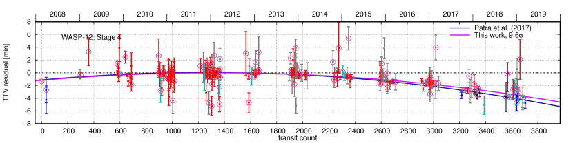
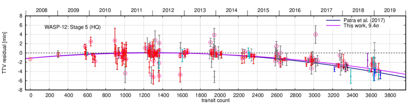
Figure 2: Transit times of WASP-12 derived in this work. Top panel is for all the TTV data (stage 4), bottom panel is for only HQ ones (stage 5). The models of the quadratic TTV trend are also plotted (for the multiplicative noise model).

We also considered the so-called regularized noise model from (Baluev, 2015), which in our conditions is almost equivalent to the ‘additive’ model. In this model, the noise is represented as a quadrature sum of the derived TTV uncertainty and of a ‘jitter’. With this model we obtain $T_{\rm d}=3.55\pm 0.31$ Myr ($3.60\pm 0.31$ Myr from only HQ TTVs), practically the same values. The best fitting TTV jitter for our data is estimated to be $20.8\pm 2.5$ sec ($18.9\pm 2.5$ sec for the HQ subsample). Therefore, this result is practically model-invariant and thus very trustable. As such, the tidal quality factor remains at $Q_{*}\sim 2\cdot 10^{5}$, the value from (Patra et al., 2017).

We did not include secondary eclipses in our analysis, and did not use some transit timings published without lightcurves that could be reprocessed. From only the transit timing data, we did not obtain any qualitatively new result for WASP-12, but RV data brought a significant additional information about the nature of this TTV trend (see Section 6).

5.5 WASP-4: yet another TTV trend?

We suspected the nonlinear trend in WASP-4, analogous to the WASP-12 one, right after the new EXPANSION lightcurves from 2017 observing season were processed. The magnitude of the trend corresponded to $T_{\rm d}\sim 10$ Myr (surprisingly close to what was recently claimed by Bouma et al. 2019). However, that time the trend interpretation depended on just a few data points from 2017. To confirm or retract the trend hypothesis we initiated in 2018 a prioritized observing campaign of WASP-4 within the EXPANSION project. By the end of 2018 we acquired $10$ new transit lightcurves.

Table 3 shows the observation log, including the EXPANSION data, as well as a few older lightcurves found in the ETD and AXA databases, and also $6$ archival lightcurves from the TRAPPIST-South telescope. This table does not include data taken from the literature ($29$ lightcurves). The total number of WASP-4 lightcurves reprocessed in this work was $66$ (plus one outlier not included in the final analysis). The trend information mainly comes from $14$ observations made in 2017-2018. Among them $10$ were taken by P. Evans with a $36$ cm Planewave CDK telescope equipped by a SBIG STT 1603-3 CCD and hosted at El Sauce Observatory, Chile. This is a good quality equipment at a good site, and the corresponding TTV measurements appeared in turn quite competitive with even TESS ones (which were released later).

Table 3: Observation log for $31$ of the WASP-4 transit lightcurves.

Obs. Date	Aperture	Filter	Cadence	Airmass	Observer
	[m]		[min]
2008-09-23		Rc	$0.46$	$1.26\longmapsto 1.03$	Fernando Tifner (AXA)
2009-09-22		Rc	$1.18$	$1.27\longmapsto 1.02$	Fernando Tifner (AXA)
2010-07-08		Rc	$1.02$	$1.11\longmapsto 1.19$	Thomas Sauer (ETD)
2010-08-17	$2.15$	Ic	$1.13$	$1.07\longmapsto 1.34$	Eduardo Fernandez-Lajus, Romina P. Di Sisto
2010-10-04		Clear	$0.46$	$1.02\longmapsto 1.15$	Gavin Milne (ETD)
2010-11-01		Rc	$0.41$	$1.03\longmapsto 1.38$	TG Tan (ETD)
2010-11-05		Clear	$0.52$	$1.13\longmapsto 1.85$	Ivan Curtis (ETD)
2010-12-20	$0.60$	‘I+z’	$0.53$	$1.14\longmapsto 2.02$	TRAPPIST
2011-09-15	$0.60$	‘I+z’	$0.33$	$1.62\longmapsto 1.04$	TRAPPIST
2011-09-27	$0.60$	Ic	$0.33$	$1.23\longmapsto 1.05$	TRAPPIST
2011-10-21	$0.60$	Ic	$0.33$	$1.04\longmapsto 1.61$	TRAPPIST
2011-12-19	$0.60$	‘I+z‘	$0.33$	$1.14\longmapsto 2.07$	TRAPPIST
2012-06-07	$0.60$	Ic	$0.35$	$1.41\longmapsto 1.03$	TRAPPIST
2012-09-11	$0.25$	Clear	$0.82$	$1.59\longmapsto 1.14$	Phil Evans
2013-09-21		Clear	$0.79$	$1.19\longmapsto 1.07$	Colazo, C. Schneiter, E. M.
2013-10-07		Rc	$0.30$	$1.41\longmapsto 1.05$	Erin Miller (ETD)
2013-12-13		Rc	$0.31$	$1.60\longmapsto 1.10$	Erin Miller (ETD)
2014-08-03	$2.15$	Clear	$3.17$	$1.10\longmapsto 1.04$	Eduardo Fernandez-Lajus, Romina P. Di Sisto
2014-08-16		Clear	$0.64$	$1.05\longmapsto 1.60$	Martin Masek (ETD)
2014-08-20	$2.15$	Ic	$6.04$	$1.01\longmapsto 1.27$	Eduardo Fernandez-Lajus, Romina P. Di Sisto
2014-08-20	$1.54$	Clear	$3.26$	$1.01\longmapsto 1.42$	Carlos Colazo, Carolina Villarreal
2014-10-25	$1.54$	Rc	$0.75$	$1.30\longmapsto 2.91$	Cecilia Quinones
2015-08-15	$2.15$	Ic	$3.05$	$1.02\longmapsto 1.22$	Eduardo Fernandez-Lajus, Romina P. Di Sisto
2017-07-26	$0.36$	Rc	$1.51$	$1.42\longmapsto 1.04$	Phil Evans
2017-09-07	$0.36$	Rc	$1.19$	$2.44\longmapsto 1.02$	Phil Evans
2017-09-23	$0.36$	Rc	$2.16$	$1.38\longmapsto 1.02$	Phil Evans
2017-09-24	$0.46$	Clear	$1.02$	$1.19\longmapsto 1.15$	H. Durantini Luca, P. Baez, C. Colazo
2018-05-23	$0.36$	Rc	$2.07$	$2.74\longmapsto 1.09$	Phil Evans
2018-06-20	$0.36$	Rc	$2.03$	$1.05\longmapsto 1.02$	Phil Evans
2018-07-25	$0.36$	Rc	$2.26$	$1.75\longmapsto 1.02$	Phil Evans
2018-08-10	$0.36$	Rc	$2.06$	$1.08\longmapsto 1.31$	Phil Evans
2018-08-12	$0.30$	Rc	$1.55$	$1.10\longmapsto 1.30$	Carl R. Knight
2018-08-14	$0.36$	Rc	$2.22$	$1.03\longmapsto 1.32$	Phil Evans
2018-08-15	$2.15$	Ic	$3.05$	$1.05\longmapsto 1.28$	Eduardo Fernandez-Lajus, Romina P. Di Sisto
2018-08-22	$0.36$	Rc	$2.12$	$1.02\longmapsto 1.51$	Phil Evans
2018-08-26	$0.36$	Rc	$2.06$	$1.02\longmapsto 1.58$	Phil Evans
2018-10-14	$0.30$	Rc	$1.61$	$1.10\longmapsto 1.29$	Carl R. Knight

Our new data did not confirm the trend: the updated TTV time series became consistent with strictly linear ephemeris, so we decided that our trend hypothesis was wrong. But Bouma et al. (2019) reported a detection of this trend based on the new TESS transit data, obtained practically simultaneously with our observations in the EXPANSION network. To shed more light on this apparent controversy, we then performed additional analysis, including the TTV data published in the literature without lightcurves and the new TESS timings. This includes very accurate transit times derived from the transmission spectroscopy by Huitson et al. (2017), transit times by Hoyer et al. (2013), by Wilson et al. (2008) and two early WASP timings given in (Gillon et al., 2009a). We did not use the HST spectral observations from Ranjan et al. (2014): these data might be inaccurate because the spectra were partly overexposed and hence the flux measurements are likely not very reliable.

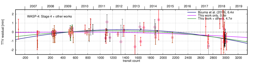
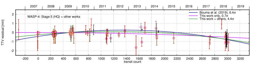
Figure 3: Transit times of WASP-4, including the homogeneous sample from this work (without DFOSC data possibly affected by clock errors), and the timing data published in literature without lightcurves. Top panel is for all the TTV data (Stage 4), bottom panel is for only HQ ones (Stage 5). Several models of the quadratic TTV trend are also plotted with the trend significance labelled in the legend (for the regularized noise model and simply merging heterogeneous TTV data).

The full TTV time series is shown in Fig. 3. Now, with the new TESS transit times added, the quadratic term of the trend indeed appears significant, according to our analysis. However, we obtain a smaller magnitude and significance than Bouma et al. (2019) reported. The trend is still not detectable with the use of only the homogeneously derived portion of TTV data from this work. That is, the information about the trend comes mainly from the third-party observations rather than from our data release. By inspecting Fig. 3 we may suspect that the trend depends primarily on just the four high-accuracy timings provided by Huitson et al. (2017). The TESS timing does not in fact contradict anything and visually they are in a satisfactory agreement with what was obtained in the EXPANSION project in 2018.

However, justifying the trend detection based on just four data points, even apparently accurate ones, might be quite dangerous. Looking into the details of the (Huitson et al., 2017) TTV data, they were based on just the linear limb-darkening model. Although the authors ensured that based on some preliminary analysis their results (including fit uncertainties) did not change significantly for linear and for more complicated limb-darkening models, we remain concerned about this. Also, we could not find a clear confirmation in the text that the red noise was taken into account when fitting the lightcurves. Although it is mentioned that some ‘systematics’ are fitted, from the description given in the text the ‘systematics’ appear to be a deterministic parametric function rather than an autocorrelated random process.

In view of this we notice that in the similar transmission spectroscopy lightcurves for WASP-12 (Stevenson et al., 2014) we robustly detect significant red noise. Inclusion of this red noise in the lightcurve model roughly doubled the derived transit timing uncertainties from $\sim 3$ sec to $\sim 5$ sec. Significant red noise was also detected in the WASP-52 transmission spectroscopy lightcurve from (Chen et al., 2017), though not detected in the HD 189733 data by Kasper et al. (2019). The latter, however, revealed the anomalous transit time discussed above. A public release of the Huitson et al. (2017) lightcurves is not available, so we did not reanalyse them in our pipeline. We therefore decided to investigate this issue using a different approach.

As it was explained above, formally declared TTV uncertainties never appear entirely accurate: the actual scatter of TTV residuals may be systematically different (usually larger). However, different teams may process data quite differently, and hence each team might have its own bias in the reported TTV uncertainties. Therefore, different portions of such a heterogeneous TTV compilation may need to be weighted differently to balance this effect. However, those weights are not known to us a priori, so they need to be estimated from the TTV data ‘on-the-fly’, e.g. based on the actually observed scatter of the TTV residuals in each homogeneous portion.

We therefore separated all our TTV data into the following four more or less homogeneous classes: (i) the ‘main’ subset including transit timings derived in this work and three old timings given in (Gillon et al., 2009a) without public lightcurve data; (ii) the rich TTV subset by Hoyer et al. (2013); (iii) the four high-accuracy timings by Huitson et al. (2017); and (iv) the TESS timings from (Bouma et al., 2019). All these data sets should have an independently fittable noise parameter.

This noise was modelled by one of two models discussed in (Baluev, 2015), namely by (i) the multiplicative model, or (ii) the so-called regularized model. These ‘noise models’ represent a parametrized model for the variance of each TTV measurement, in which a single free parameter regulates the weight of the corresponding TTV data set as a whole. Since this approach involves a separate and largely independent treatment of each TTV data set, we call this as ‘separated’ model of the TTV data. It can be fitted by using the maximum-likelihood method, as discussed in (Baluev, 2009). In such a way the relative weighting of different TTV subsets is determined adaptively and basically tied to the corresponding TTV residuals RMS.

For a comparison, we also analysed the TTV data plainly merged into a single time series without any relative weighting. This analysis was also performed for the same two noise models, multiplicative and regularized ones. The TTV trend itself was always modelled by the quadratic function (5) with three free coefficients.

As we expected, it appeared that the magnitude of the quadratic term and especially its derived uncertainty is sensitive to the choice of the noise model. In the case of a ‘separated’ model the trend uncertainty gets increased. Therefore, by allowing some TTV data to be actually less accurate than stated, the significance of the trend may reduce. For example, it may reduce if the four Huitson et al. (2017) transit times are less accurate than formally stated. And because of the small number of these data (just the four), their RMS does not constrain the noise level well, so this level can be varied relatively freely.

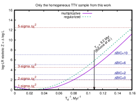
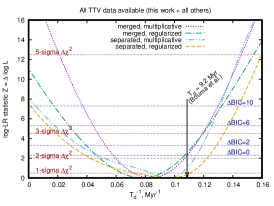
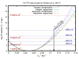
Figure 4: Logarithm of the likelihood ratio statistic for WASP-4, $Z(q)$, as a function of $q=T_{\rm d}^{-1}$. Three graphs correspond to different compilations of TTV data (homogeneous from this work / all / all but Huitson et al. (2017)). The curves within each graph correspond to different models of the TTV noise (merged/separated and multiplicative/regularized). In each graph a set of the significance threshold levels is also shown, corresponding to the frequentist $\chi^{2}$ test or to the Bayesian information criterion (BIC). See text for more details.

In Fig. 4, we demonstrate this effect in the shape of the likelihood function $\mathcal{L}$. For this goal we consider the log-likelihood-ratio statistic $Z$ determined in accordance with (Baluev, 2009). We compute (i) the global maximum of the likelihood function $\mathcal{L}_{\max}$ with respect to all the noise parameters and all three TTV trend coefficients, and (ii) the value $\mathcal{L}_{\max}^{\prime}(q)$ maximized with respect to all parameters except for the quadratic coefficient $dP/dn=P^{2}T_{\rm d}^{-1}=qP^{2}$, where $q=T_{\rm d}^{-1}$ was fixed prior to the fit. The quantity $Z(q)=\log[\mathcal{L}_{\max}/\mathcal{L}_{\max}^{\prime}(q)]$ therefore indicates whether the given $q$ is statistically consistent with the best-fitting value $\hat{q}$ which corresponds to the global maximum $\mathcal{L}_{\max}$. We always have $Z(q)\geq 0$, and the larger is $Z$, the more statistically significant is the deviation of $q$ from $\hat{q}$ and the less consistent with the data this $q$ is. If our models are linearisable than $Z(q)$ should have an almost parabolic shape with a single minimum at $\hat{q}$.

We use two approaches to calibrate the levels of $Z(q)$, both rely on the assumption that the model is linearisable and hence $Z(q)$ is quadratic (while the likelihood ratio $\exp(-Z(q))$ is Gaussian). The first approach is the frequentist $\chi^{2}$ test, and the second one is the Bayesian Information Criterion (BIC). In the frequentist treatment, the significance level of a given $Z$ is approximately the $\chi^{2}_{1}(2Z)$, or the $\chi^{2}$-distribution with $d=1$ degree of reedom (one degree because we have just one free parameter $q$ left in $Z(q)$). This would mean that the significance level for a given $q$ would correspond to $\sqrt{2Z}$ in the $n$-sigma notation, or vice versa, any $n$-sigma significance level would correspond to the threshold level $Z(q)=n^{2}/2$.

The BIC is defined as ${\rm BIC}=2\log\mathcal{L}-k\log N$, where $k$ is the total number of free parameters in the model, and $N$ is the number of observations (number of transit times). To compare different models with $k_{1}$ and $k_{2}$ parameters we use the difference $\Delta{\rm BIC}=2Z-d\log N$ with $d=k_{1}-k_{2}=1$ in our case. Hence, the significance threshold for $Z(q)$ becomes $Z=(\Delta{\rm BIC}+\log N)/2$. Here $\Delta{\rm BIC}$ is deemed to be an input parameter determining the requested significance level (typical practical values are $2$, $4$, $6$, $10$).

The special value $Z(0)$ indicates the significance of the nonlinear trend itself (i.e. how much $q=0$ is consistent with the data, with the adopted TTV noise model).

In Fig. 4, we plot this statistic $Z(q)$ for three TTV data compilations, including (i) only the homogeneous data from this work, (ii) all TTV data, (iii) all TTV data excluding (Huitson et al., 2017), and for all our noise models, including (i) the plain merging of heterogeneous datasets and (ii) adaptive merging of heterogeneous datasets with individually fittable noise parameters. For each of these model layouts we adopt either a multiplicative or regularized noise model, defined in (Baluev, 2015).

As we can see, the shape of the likelihood function may change a lot depending on the model and TTV data involved. We can draw the following conclusions:

1. Our homogeneously derived TTV data do not support the existence of any quadratic trend. These data are consistent with a linear ephemeris below $1$-sigma level.

2. Simultaneously, the value of $T_{\rm d}=9.2$ Myr from (Bouma et al., 2019) seems too poorly consistent with our homogeneous TTV subsample, at the level above $3$-sigma in terms of the $\chi^{2}$ test or with $\Delta{\rm BIC}\sim 4-6$ (depending on the model). We believe this may appear, at least in some part, because Bouma et al. (2019) did not take into account the heterogeneous nature of the TTV data, merging them into a single time series.

3. Joining our data with the remaining third-party TTV measurements allows us to refine the localization of the parameter $q$ greatly and even suggests that this $q$ can be significantly non-zero. However, the significance of this conclusion, as well as possible confidence ranges for $q$ appear very model dependent. If we plainly merge all the TTV data, we obtain that $q$ is inconsistent with zero at the high $\sim 5-7$-sigma level. But using our adaptive separated noise model, this significance drops to merely $3-4$-sigma.

4. The shape of the likelihood function becomes significantly non-parabolic in the case of our adaptive separated noise model. This indicates that this model may be too non-linear and therefore our significance estimates may appear inaccurate. It may even appear that the significance of the trend is reduced even further below the $3-4$-sigma level mentioned above.

5. The most trustable and model-stable behaviour appears when we just remove the TTV data by Huitson et al. (2017). Then $Z(q)$ behaves as a nice parabolic function, indicating an almost-linear model and nearly Gaussian likelihood. In this case, the quadratic trend has the significance $2.8-3$-sigma or $\Delta{\rm BIC}\sim 4$, which is very remarkable but still needs further confirmation by more observations. The magnitude of the best fitting trend then becomes $T_{\rm d}\sim 20$ Myr with large uncertainty. Curiously, the value of $T_{\rm d}=9.2$ Myr given by Bouma et al. (2019) appears in this case even less likely than the no-trend model ($T_{\rm d}=\infty$).

6. In any case, the trend magnitude is very uncertain, while its confidence ranges appear very asymmetric and non-Gaussian in the separated noise model. The value $T_{\rm d}=9.2$ Myr given in (Bouma et al., 2019) looks more like a lower limit on $T_{\rm d}$, while the actual value may reach even $\sim 100$ Myr, given the large uncertainty of this parameter.

Therefore the putative TTV trend magnitude and the detection significance for WASP-4 are severely model-dependent. They solely depend on how we treat the heterogeneous nature of the TTV data. Moreover, as recognized by Bouma et al. (2019), $T_{\rm d}$ as small as $9.2$ Myr is inconsistent with theoretical predictions of the tidal quality parameter. Given our discussion, we believe that it is too early to definitely claim the detection of this trend until more homogeneous TTV data are collected. At least, it is too early to claim that this object breaks any theoretical predictions. However, WASP-4 remains a very interesting target that may indeed hide serendipitous discoveries.

6 Self-consistent analysis of radial velocity and transit data

Below we layout our goals related for the self-consistent analysis of radial velocity and transit data.

1. Derive a more complete set of parameters in a self-consistent model, in particular planetary masses and physical radii (rather than merely the planet/star radii ratio).

2. Derive a more realistic fit of GJ 436 b, taking into account its significant orbital eccentricity.

3. For WASP-12 and WASP-4, test whether their (possible) TTV trends could appear through the light-travel effect, caused by the gravity of a distant unseen companion.

4. Derive the rotation parameters of the stars via the Rossiter-McLaughlin (hereafter RM) effect, and test how much it is sensitive to the correction coeffiecients suggested in (Baluev & Shaidulin, 2015).

Notice that even the combination of transit and radial velocity data does not allow to determine the star mass from a self-consistent fit. The information about the star mass usually comes from astrophysical models of stellar spectra, e.g. based on stellar evolutionary tracks. Such models in fact provide certain constraints on the stellar mass $M_{\star}$ and radius $R_{\star}$ that can be used to provide an entirely self-consistent global fit. However, in this work we were more interested to estimate the uncertainties inferred by the transit and radial velocity data, so we still prefer not to mix them with the uncertainties of astrophysical models that may also contain an additional systematic error.

Table 4: Star masses adopted in the joint transit+RV fits.

host star	$M_{\star}[M_{\odot}]$	reference
Corot-2	$0.97(6)$	Alonso et al. (2008)
GJ436	$0.452\left(+14\atop-12\right)$	Torres et al. (2008)
HAT-P-13	$1.22\left(+5\atop-10\right)$	Bakos et al. (2009)
HD189733	$0.806(48)$	Torres et al. (2008)
TrES-1	$0.878\left(+38\atop-40\right)$	Torres et al. (2008)
WASP-2	$0.84\left(+11\atop-12\right)$	Triaud et al. (2010)
WASP-3	$1.24\left(+6\atop-11\right)$	Pollacco et al. (2008)
WASP-4	$0.930\left(+54\atop-53\right)$	Triaud et al. (2010)
WASP-5	$1.000\left(+63\atop-64\right)$	Triaud et al. (2010)
WASP-6	$0.88\left(+5\atop-8\right)$	Gillon et al. (2009b)
WASP-12	$1.434\left(+110\atop-90\right)$	Collins et al. (2017)
XO-2N	$0.96(5)$	Damasso et al. (2015)
XO-5	$0.88(3)$	Pál et al. (2008)

Therefore, we fixed certain ‘reference’ values of $M_{\star}$ for our ten targets, as given in Table 4. We did not take into account the stated uncertainties of $M_{\star}$ when computing our fits. In case if the adopted $M_{\star}$ is different from the reference value, the fit can be easily rebased to another $M_{\star}^{\prime}$ based on the following simple laws:

$$R_{\star}^{\prime} = R_{\star}\left(M_{\star}^{\prime}/M_{\star}\right)^{\frac{1}{3}},$$

$$r_{\rm pl}^{\prime} = r_{\rm pl}\left(M_{\star}^{\prime}/M_{\star}\right)^{\frac{1}{3}},$$

$$a^{\prime} = a\left(M_{\star}^{\prime}/M_{\star}\right)^{\frac{2}{3}},$$

$$m_{\rm pl}^{\prime}\sin i^{\prime} = m_{\rm pl}\sin i\left(M_{\star}^{\prime}/M_{\star}\right)^{\frac{1}{3}},$$

$$\cos i^{\prime} = \cos i\left(M_{\star}^{\prime}/M_{\star}\right)^{-\frac{1}{3}}.$$ (7)

The first formula of this list comes from the known property that a transit fit actually constrains the star density $\rho_{\star}\propto M_{\star}R_{\star}^{-3}$, rather than $R_{\star}$ or $M_{\star}$ separately (Mandel & Agol, 2002). The second one appears because the transit data constrain the ratio $r_{\rm pl}/R_{\star}$, so the scaling law of $r_{\rm pl}$ is the same as for $R_{\star}$. The third and the fourth formulae for the orbital semimajor axis and planetary mass, respectively, follow from the basic properties of the Doppler method and can be found e.g. in (Baluev, 2013). The last relationship for cosine of orbital inclination $i$ follows because $i$ is constrained by only the transit data, via the measured impact parameter $b=a\cos i/R_{\star}$, so the scale law for $\cos i$ corresponds to $R_{\star}/a$. The last two formulae can be combined together to obtain

$$m_{\rm pl}^{\prime}=m_{\rm pl}\frac{\left(M_{\star}^{\prime}/M_{\star}\right)^{\frac{1}{3}}}{\sqrt{1+\left(1-\left(M_{\star}^{\prime}/M_{\star}\right)^{-\frac{2}{3}}\right)\mathop{\text{cotan}}\nolimits^{2}i}}.$$ (8)

Since $\mathop{\text{cotan}}\nolimits i$ is below $0.15$ for all our targets, the term beneath the square root represents only a negligible correction. Some scale formulae above are not entirely accurate, neglecting certain second-order corrections, but since the values of $M_{\star}$ for all our targets are now restricted to quite narrow ranges, the practical accuracy of (7,8) should be satisfactory.

To perform the self-consistent analysis, for the transit data we used basically the same model as above, except that the planet motion was assumed Keplerian rather than circular. The radial velocity for each target was modelled by the Keplerian curve plus a linear trend (to account e.g. for possible long-period companions in the system). We also include a quadratic term in the planetary longitude, to take into account possible TTV trends, see (Baluev, 2018).

For many of our targets, the RV data contained substantial in-transit runs, obviously aimed to detect the RM effect. For these targets we therefore included in our compound RV model the RM effect based on the approach by Baluev & Shaidulin (2015). To accurately approximate this effect, we must know some effective values of the limb-darkening coefficients $A_{\rm RV}$ and $B_{\rm RV}$, corresponding to the Doppler spectral range. Also, we need to specify two correction coefficients $\nu$ and $\mu$ that depend on the average characteristics of spectral lines and on the method used to derive the radial velocity from the spectrum. But unfortunately, these four quantities are too difficult to derive reliably from the spectra themselves. Instead, it is reasonable to treat them as fittable parameters of the RV model. However, in such a case the model becomes nearly degenerate, because as discussed in (Baluev & Shaidulin, 2015), the parameters $\nu$ and $\mu$ are strongly correlated with $A$ and $B$. We therefore adopted the following hybrid approach. First, we assumed that $A_{\rm RV}$ and $B_{\rm RV}$ are equal to the corresponding values of the photometric data obtained with a clear aperture. Concerning $\nu$ and $\mu$, we considered them separately for different instruments. This should take into account possible corrections of the RM effect, jointly with possible inaccuracies of the limb-darkening coefficients, on a per-instrument basis.

When computing the fits, we treated separately the RV data obtained at different instruments. Moreover, if the RV data belonging to the same instrument contained in-transit pieces, we separated these portions of the data from each other and treated them as individual RV data sets. This might make the model more adequate, because e.g. the scatter of the RV residuals within each such short run covering just a few hours is significantly smaller than for the entire dataset covering years. This is essentially the impact of red noise in the RV data. Also, the red noise may result in a small individual offset of each in-transit run.

For some targets we also found several compact series of out-of-transit runs covering just a single night. Such portions of the RV data were treated separately too, with an individual offset and individual noise parameters. After performing a preliminary fit of the joint transit+RV model described above, we run the red-noise detection algorithm described above for transit data, but now we extended it to all the RV data sets as well.

For Corot-2, WASP-4, and WASP-12 we computed an additional alternative fit without splitting the RV data belonging to the same instrument. In this case, possible RV offsets between different compact runs were taken into account implicitly, via a single red noise model of the merged data set. All the analysis was performed with the PlanetPack software of version 3 (Baluev, 2018).

We separate our results in two parts: Table 5 gives some most important non-planetary parameters of our fits, and Table 6 contains only planetary parameters. The tables are presented here in a reduced form; their expanded versions that include e.g. RM correction coefficients can be found in the online-only supplement.

First of all, we notice that the RM correction coefficients $\nu$ and $\mu$ are usually consistent with zero, given their uncertainties. We found only the following targets convincingly demonstrating significant nonzero values: Corot-2 ($\mu$ for the HARPS RV data), HD 189733 ($\nu$ for Keck/HIRES and SOPHIE, and $\mu$ for HARPS, HARPSN, and Keck/HIRES), WASP-5 ($\mu$ for HARPS), and possibly GJ 436 ($\nu$ for GJ 436 HARPS, HARPSN, Keck/HIRES). In theory, $\nu$ should usually be zero, since most our RV data were derived with TERRA, which is a kind of a spectrum modelling method (Anglada-Escudé & Butler, 2012). A nonzero $\nu$ may appear only if the RV data were derived by the cross-correlation technique, and simultaneously the spectral lines have some asymmetry on average (Baluev & Shaidulin, 2015). Since this is not the case for the most targets, a few significantly nonzero $\nu$ estimates may indicate that the adopted limb-darkening coefficients $A_{\rm RV}$ and $B_{\rm RV}$ are inaccurate for the relevant RV dataset. In such a case, the value of $v\sin i$ and $\lambda$ may involve an additional bias which is difficult to estimate without a better guess for $A_{\rm RV}$ and $B_{\rm RV}$.

Even though we did not detect here very many occurrences of significantly nonzero RM correction coefficients, it is still important to preserve them in the RV model as free parameters, in order to have a more realistic (increased) uncertainty in $v\sin i$ and $\lambda$, as well as in other RV-derived parameters, like e.g. the RV trends.

Table 5: Self-consistent fits of transit and radial velocity data: stellar parameters and RV trends.

host star	rad. accel.	star radius	rotation vel.	spin-orbit ang.
	$c_{1}$ [m/s/yr]	$R_{\star}\ [R_{\odot}]$	$v\sin i$ [m/s]	$\lambda\ [^{\circ}]$
Corot-2	$-74(11)$	$0.925(19)$	$8930(400)$	$3.1(6.6)$
Corot-2’	$-0.5(3.1)$	$0.885(29)$	$8570(430)$	$3.0(8.2)$
GJ436	$0.02(11)$	$0.4266(89)$	$1800(1000)$	$354.5(4.9)$
HAT-P-13	$17.2(1.0)$	$1.691(25)$	$2300(1100)$	$359.5(5.5)$
HAT-P-13’	$17.56(85)$	$1.692(25)$	$2600(1300)$	$0.0(5.4)$
HD189733	$-1.07(75)$	$0.7583(31)$	$2280(110)$	$0.08(36)$
TrES-1	$-1.9(1.4)$	$0.819(13)$	—	—
WASP-2	$-3.9(1.8)$	$0.8200(82)$	$960(850)$	$345(18)$
WASP-3	$-7.9(2.7)$	$1.337(28)$	—	—
WASP-4	$-0.7(1.1)$	$0.9029(43)$	$1890(220)$	$344(16)$
WASP-4’	$-0.8(1.2)$	$0.9045(46)$	$1890(220)$	$343(16)$
WASP-5	$-0.03(78)$	$1.127(16)$	$2470(400)$	$0.2(6.4)$
WASP-6	$-420(260)$	$0.829(23)$	$1620(130)$	$352(11)$
WASP-12	$-5.4(2.0)$	$1.657(12)$	$600(1200)$	$9(48)$
WASP-12’	$-7.5(2.2)$	$1.660(16)$	$1300(1500)$	$75(30)$
XO-2N	$-1.2(1.2)$	$0.986(14)$	—	—
XO-5	$1.3(1.2)$	$1.068(51)$	—	—

The fitting uncertainties are given in parenthesis after each estimation, in the units of the last few figures. The star mass from Table 4 was assumed constant here and its uncertainties were not included in the fit. Using the full set of transits for GJ436, while only the HQ (Stage 5) transits for other targets. A stroke stands for an alternative fit computed without splitting the RV data belonging to the same instrument (see text).

Table 6: Self-consistent fits of transit and radial velocity data: planetary parameters.

host star	planet mass	planet radius	orbital period1	TTV trend1,2,3	mean longitude1	inclination	eccentricity	pericenter arg.
	$m_{\rm pl}\ [M_{\rm Jup}]$	$r_{\rm pl}\ [R_{\rm Jup}]$	$P$ [d]	$T_{\rm d}$ [Myr]	$l\ [^{\circ}]$	$i\ [^{\circ}]$	$e$	$\omega\ [^{\circ}]$
Corot-2	$2.744(51)$	$1.523(36)$	$1.74299686(44)$	$-11.2(9.4)$	$359.4(1.6)$	$88.15(56)$	$0.042(18)$	$60(18)$
Corot-2’	$2.85(10)$	$1.455(51)$	$1.74299682(45)$	$-10.4(8.2)$	$0.7(2.4)$	$88.32(52)$	$0.013(26)$	$320(130)$
GJ436	$0.06896(56)$	$0.3581(97)$	$2.64389856(36)$	$7.1(3.2)$	$335.82(44)$	$86.83(10)$	$0.1666(57)$	$324.9(2.4)$
HAT-P-13 b	$0.8528(59)$	$1.465(30)$	$2.9162384(17)$	$-2.42(86)$	$158.64(41)$	$82.12(22)$	$0.0126(46)$	$219(29)$
HAT-P-13 c	$14.17(28)$	—	$446.32(24)$	—	$63.99(18)$	—	$0.6621(58)$	$175.28(37)$
HAT-P-13’ b	$0.8532(53)$	$1.466(30)$	$2.9162383(17)$	$-2.41(85)$	$158.58(35)$	$82.10(22)$	$0.0117(41)$	$218(28)$
HAT-P-13’ c	$14.16(25)$	—	$446.29(21)$	—	$63.99(16)$	—	$0.6614(50)$	$175.28(32)$
HD189733	$1.1542(74)$	$1.1840(52)$	$2.218575123(57)$	$28(12)$	$20.45(38)$	$85.712(36)$	$0.0028(38)$	$62(64)$
TrES-1	$0.6967(82)$	$1.122(22)$	$3.03006960(18)$	$-5.7(9.5)$	$298.67(49)$	$88.69(28)$	$0.003(12)$	$263(86)$
WASP-2	$0.8711(73)$	$1.087(14)$	$2.15222163(67)$	$-12(11)$	$214.37(25)$	$84.82(10)$	$0.0134(56)$	$253(11)$
WASP-3	$1.982(49)$	$1.419(32)$	$1.84683480(30)$	$-11.1(5.5)$	$274.88(83)$	$84.24(32)$	$0.010(15)$	$41(74)$
WASP-4	$1.1949(65)$	$1.3915(82)$	$1.338231501(75)$	$47(45)$	$235.80(26)$	$88.63(30)$	$0.0068(35)$	$258(20)$
WASP-4’	$1.1976(68)$	$1.3940(86)$	$1.338231501(75)$	$47(45)$	$235.87(26)$	$88.63(30)$	$0.0053(38)$	$247(28)$
WASP-5	$1.5351(80)$	$1.294(25)$	$1.6284311(14)$	$5.2(6.3)$	$343.01(32)$	$84.57(33)$	$0.0086(46)$	$66(22)$
WASP-6	$0.458(20)$	$1.175(35)$	$3.36100264(65)$	$14(14)$	$32.6(2.4)$	$89.00(36)$	$0.036(24)$	$116(36)$
WASP-12	$1.422(14)$	$1.953(15)$	$1.091421080(96)$	$3.46(24)$	$37.00(51)$	$81.86(16)$	$0.0259(74)$	$250(11)$
WASP-12’	$1.413(15)$	$1.956(20)$	$1.091421078(96)$	$3.47(24)$	$36.82(49)$	$81.96(18)$	$0.024(11)$	$252(11)$
XO-2N	$0.5924(68)$	$1.017(16)$	$2.61585963(16)$	$80(140)$	$198.72(48)$	$88.33(25)$	$0.008(13)$	$91(29)$
XO-5	$1.050(15)$	$1.061(67)$	$4.1877477(38)$	$-1.82(68)$	$83.5(1.2)$	$86.82(51)$	$0.009(12)$	$200(94)$

Same comments as in Table 5 also apply here.

¹These parameters refer to $T_{0}=2455197.5$ (1 Jan, 2015) in the BJD TDB system.

²Except for WASP-12 case, the uncertainties for $T_{\rm d}$ are rather formal here, because this parameter becomes very nonlinear and non-Gaussian whenever it is comparable to the uncertainty. The linear parameter is $q=1/T_{\rm d}=-\dot{P}/P$ with the uncertainty $\sigma_{q}=\sigma_{T_{\rm d}}/T_{\rm d}^{2}$.

³The realistic uncertainty in $T_{\rm d}$ also depends on the observed TTV scatter $\chi_{\rm TTV}^{2}$ from Table 2, see Section 5.3.

Now let us consider the putative RV trends (radial accelerations). They are modelled by a linear function

$${\rm RV}=c_{0}^{\prime}+c_{1}(t-t_{0}),$$ (9)

where $c_{0}^{\prime}$ is a dataset-specific RV offset, and $c_{1}$ is the trend coefficient (common for all datasets).

If not an instrumental effect or some long-term astrophysical variation, this trend can be explained through a gravitational effect from a distant unseen companion. But such a companion would also affect the observed transit times via the light-travel effect. Basically, the light-travel effect is determined by the position of the inner star-planet system along the line of sight, which equals to the integral of the RV trend. Therefore, the transit time delay (TTD) corresponding to (9) would be:

$${\rm TTD} = \mathop{\text{const}}\nolimits+\frac{c_{0}}{\mathcal{C}}(t-t_{0})+\frac{c_{1}}{\mathcal{C}}\frac{(t-t_{0})^{2}}{2}$$ (10)

$$= \mathop{\text{const}}\nolimits+\frac{Pc_{0}}{\mathcal{C}}(n-n_{0})+\frac{P^{2}c_{1}}{\mathcal{C}}\frac{(n-n_{0})^{2}}{2},$$

where $\mathcal{C}$ is the speed of light. This formula becomes mathematically identical to the quadratic TTV trend (5). But now the second term in (10) with $c_{0}$ (the absolute RV) represent a minor Doppler-like correction of the orbital period $P$, while $c_{1}$ is basically the same TTV effect as observed e.g. for WASP-12.

Now, we simply have $T_{\rm d}=\mathcal{C}/c_{1}$. Taking into account the adopted measurement units,

$$T_{\rm d}[{\rm Myr}]\simeq-\frac{300}{c_{1}[{\rm m}\,{\rm s}^{-1}\,{\rm yr}^{-1}]}.$$ (11)

The minus sign appears because the positive RV trend means increasingly late light arrival (apparent delay of the transits, as if the planet was spiraling out).

We found the statistically significant RV trend in the Corot-2, about $-74\pm 11$ m/s per year. However, this trend can also be a hidden red-noise effect, because it disappears in the alternative fit without splitting the HARPS data per subsets. One of the HARPS subsets appeared to have just seven observations, so the “split” fit might appear rather unreliable statistically. Finally, we found several RV outliers for Corot-2, possibly indicating some hidden anomalies in its spectrum that suggest potential inaccuracies of the derived Doppler information. Therefore, we conclude that the suspected radial acceleration in Corot-2 remains controversial and needs further confirmation.

For Corot-2, the formula above implies $T_{\rm d}=(4.0\pm 0.6)$ Myr, or $q=T_{\rm d}^{-1}\sim(0.25\pm 0.04)$ Myr^-1. The current TTV data are unable to reliably detect such a trend. Finally, from the transit times we obtain $q\sim-0.1\pm 0.1$. The difference from the RV estimate of $q$ is inconclusive given the high level of model dependency. Nonetheless, Corot-2 remains an interesting target for further monitoring, because it may provide the first detection of an unseen object simultaneously by Doppler and Roemer effects.

Contrary to Corot-2, in WASP-12 we detect a more model-stable radial acceleration about $-5$ or $-8$ m/s/yr, depending on the model. The trend information mainly comes from the rich set of SOPHIE data available for this target ($>100$ points). The RV trend looks rather reliable given its uncertainty, so the “observed” $T_{\rm d}$ need to be cleaned from the non-tidal portion. This is performed in Sect. 7 below.

For WASP-4, the RV trend estimation is consistent with zero, but given the uncertainty it may be as small as $-4$ m/s/yr (the three-sigma limit). This infers a TTV trend with $T_{\rm d}\sim 70$ Myr, which is consistent with the observed transit times within two sigma (see third panel in Fig. 4). Therefore, we cannot conclusively rule out or confirm the tidal nature of the putative WASP-4 TTV trend, even if this trend exists. More Doppler observations are needed to rule out the Roemer effect interpretation, or to determine in which fraction this TTV trend can be explained so. Using the same method as for WASP-12 (see Sect. 7), we obtain for WASP-4 an estimate of the tidal portion of the TTV trend of $q^{\rm tidal}=(0.019\pm 0.025)$ Myr^-1, again a statistically insignificant value.

Yet another candidate with radial acceleration is WASP-3 ($-8$ m/s/yr), but it has just $13$ RV measurements. Also, HAT-P-13 has an RV trend about $18$ m/s/yr, established long ago (Winn et al., 2010). Neither of these cases can be verified by TTV due to the lack of data.

Concerning the search of possible periods in the RV residuals, we leave this for a future work. But here we confirm that Corot-2, HAT-P-13, WASP-4, and WASP-12 reveal no hints of periodicity, so the corresponding RV trend estimations should not be affected by such signals. Also, no residual variations were detected, including trends, in the updated RV data for GJ 436 (though a spurious RV trend appeared in the older data release by Baluev et al. 2015).

7 Truly tidal portion in the WASP-12 TTV trend

According to (Bechter et al., 2014), WASP-12 is a member of a triple star system. It has a stellar companion which appears as binary itself. The total mass of these two components B and C is $0.75M_{\odot}$, and they may induce the radial acceleration of up to $0.33$ m/s/yr on the primary star (Bailey & Goodman, 2019). Therefore, the radial acceleration of $-7.5$ m/s/yr would definitely belong to some other unseen companions, possibly other distant planets, or brown dwarfs, or even to an unresolved cool star.

Whatever object or multiple objects induced this radial acceleration, they should also induce a quadratic TTV trend according to the formula (10). Notice that even if the RV trend was not significant at all, we should include it in the model in order to determine a more realistic uncertainty of the tidal part of $T_{\rm d}$. Our RV trend estimation implies the same sign as the observed cumulative value of $dP/dn$, so the tidal portion is smaller than the total observed TTV. To determine how much it is smaller, and how uncertain this value is, we perform a brief additional calculation.

First of all, we notice that information about the RV and TTV trends comes from qualitatively different observations: either solely from RV data, or solely from transit timings. Therefore, we may expect that these two quantities are practically uncorrelated (even though some negligible correlation may appear because e.g. the planetary orbital period $P$ is shared between the RV and transit data). Thanks to this property, the corresponding trend coefficients may be treated independently from each other.

In terms of the TTV trend, its magnitude is defined by $q=T_{\rm d}^{-1}$, where $T_{\rm d}$ from Table 6 is $(3.47\pm 0.24)$ Myr. Here we notice again that this uncertainty is likely underestimated by the factor of $\sqrt{\chi^{2}_{\rm TTV}}$ from Table 2, or $1.33$. Therefore, a more realistic estimate is $T_{\rm d}=(3.47\pm 0.32)$ Myr. The radial acceleration $c_{1}$ is estimated in Table 5. Based on the Corot-2 example, we believe that the alternative fit WASP-12’ is more realistic in terms of the RV trend, because in the basic fit (for split RV data) the estimated radial acceleration may also include a local red noise effect appearing within individual short in-transit runs. We do not expect that the estimated $c_{1}$ value may have any significant escaped random uncertainty, since the stellar activity was already modelled through the white and red RV jitter. Based on the formula (11), from $c_{1}=(-7.5\pm 2.2)$ m/s/yr we obtain the apparent orbital decay time $T_{\rm d}^{\rm RA}=(40\pm 12)$ Myr.

The tidal part of the TTV trend is then defined as:

$$\frac{1}{T_{\rm d}^{\rm tidal}}=\frac{1}{T_{\rm d}}-\frac{1}{T_{\rm d}^{\rm RA}}.$$ (12)

Since $T_{\rm d}$ and $T_{\rm d}^{\rm RA}$ are practically uncorrelated, this formula yields an estimation $T_{\rm d}^{\rm tidal}=(3.80\pm 0.40)$ Myr. Therefore, the truly tidal orbital decay time is $\sim 10$ per cent larger than the observed (apparent) $T_{\rm d}$, and also it has a larger uncertainty. Although the bias is only $\sim 1\sigma$, the increase of the uncertainty is noticeable.

In this work we did not consider the alternative explanation of the WASP-12 TTV via the apsidal precession (Patra et al., 2017), although this model should also be corrected for the nontidal part of the TTV.

8 Conclusions and discussion

The main conclusion of our work is that TTV data present in published literature are significantly inhomogeneous. Therefore, they cannot be plainly processed by merging them with each other. Substantial efforts must be made to increase the degree of homogeneity of the TTV data by reprocessing the archival lightcurves, or by employing sophisticated noise models separating different TTV subsets from each other. A lack of careful analysis of heterogeneous TTV data may prove dangerous, potentially leading to spurious analysis artefacts. In view of this it appears necessary to always verify our conclusions against different data models, in order to gain an impression of how much they are model-dependent.

For the particular cases of WASP-12 and WASP-4 we notice that the Roemer effect induced by possible additional companions may cause biased interpretation of the results. In particular, the apparent value of the TTV trend may appear biased, and even mimicking tidal phenomena. The Doppler observations are crucial in verifying such cases. In particular, they may help to assess a more realistic uncertainty of the truly tidal part of a TTV trend. Note that even if the RV trend estimation is consistent with zero it is important to keep it as a free parameter, because its uncertainty increases the uncertainty in the tidal portion of a TTV.

When performing the lightcurve analysis, the primary nuisance effect that currently remains rather poorly modelled is the spot activity that implies anomalies in the transit curve. It induces an additional TTV noise, which is difficult to predict or assess, except through the post-hoc estimation of the TTV scatter. Various self-consistent (“global”) fits that avoid using transit times as intermediate data do not include, as a rule, the spot-transit effect in their uncertainties. To further improve their quality, we need to spend more efforts to reducing the spot-transit event, e.g. to perform some kind of their automated detection followed by a dedicated fitting or removing the associated piece of a lightcurve. In our work the red noise model did not appear effective enough in removing the effect of spot-transit anomalies, since from the statistical point of view such anomalies may behave closer to a blue noise rather than red one.

We also consider the limb-darkening coefficients by Claret & Bloemen (2011), and conclude that their FCM versions are rather accurate, though there is a detectable remaining bias in the coefficient $B$ of about $0.1$. The LF version of these coefficients is rather poor for practical use, as well as the older coefficients from (Claret, 2000, 2004).

References

- Agol & Fabrycky (2017) Agol E., Fabrycky D. C., 2017, in Deeg H. J., Belmonte J. A., eds, , Handbook of Exoplanets. Springer, Cham
- Albrecht et al. (2012) Albrecht S., et al., 2012, ApJ, 757, 18
- Alonso et al. (2008) Alonso R., et al., 2008, A&A, 482, L21
- Anglada-Escudé & Butler (2012) Anglada-Escudé G., Butler R. P., 2012, ApJS, 200, 15
- Bailey & Goodman (2019) Bailey A., Goodman J., 2019, MNRAS, 482, 1872
- Bakos et al. (2006) Bakos G. A., et al., 2006, ApJ, 650, 1160
- Bakos et al. (2009) Bakos G. A., et al., 2009, ApJ, 707, 446
- Baluev (2008) Baluev R. V., 2008, MNRAS, 385, 1279
- Baluev (2009) Baluev R. V., 2009, MNRAS, 393, 969
- Baluev (2013) Baluev R. V., 2013, Astron. & Comp., 2, 18
- Baluev (2015) Baluev R. V., 2015, MNRAS, 446, 1493
- Baluev (2018) Baluev R. V., 2018, Astron. & Comp., 25, 221
- Baluev & Shaidulin (2015) Baluev R. V., Shaidulin V. S., 2015, MNRAS, 454, 4379
- Baluev et al. (2015) Baluev R. V., et al., 2015, MNRAS, 450, 3101
- Bean et al. (2008) Bean J. L., et al., 2008, A&A, 486, 1039
- Bechter et al. (2014) Bechter E. B., et al., 2014, ApJ, 788, 2
- Bouma et al. (2019) Bouma L. G., et al., 2019, AJ, 157, 217
- Brown et al. (2018) Brown A. G. A., Vallenari A., Prusti T., de Bruijne J. H. J., Babusiaux C., Bailer-Jones C. A. L., et al., 2018, A&A, 616, A1
- Bryan et al. (2012) Bryan M. L., et al., 2012, ApJ, 750, 84
- Cáceres et al. (2009) Cáceres C., Ivanov V. D., Minniti D., Naef D., Melo C., Mason E., Selman F., Pietrzynski G., 2009, A&A, 507, 481
- Chan et al. (2011) Chan T., Ingemyr M., Winn J. N., Holman M. J., Sanchis-Ojeda R., Esquerdo G., Everett M., 2011, AJ, 141, 179
- Chen et al. (2017) Chen G., Pallé E., Nortmann L., Murgas F., Parviainen H., Nowak G., 2017, A&A, 600, L11
- Claret (2000) Claret A., 2000, A&A, 363, 1081
- Claret (2004) Claret A., 2004, A&A, 428, 1001
- Claret & Bloemen (2011) Claret A., Bloemen S., 2011, A&A, 529, A75
- Collins et al. (2017) Collins K. A., Kielkopf J. F., Stassun K. G., 2017, AJ, 153, 78
- Damasso et al. (2015) Damasso M., et al., 2015, A&A, 575, A111
- Eastman et al. (2010) Eastman J., Siverd R., Gaudi B. S., 2010, PASP, 122, 935
- Fernandez et al. (2009) Fernandez J. M., Holman M. J., Winn J. N., Torres G., Shporer A., Mazeh T., Esquerdo G. A., Everett M. E., 2009, AJ, 137, 4911
- Foreman-Mackey et al. (2017) Foreman-Mackey D., Agol E., Ambikasaran S., Angus R., 2017, AJ, 154, 220
- Fulton et al. (2011) Fulton B. J., Shporer A., Winn J. N., Holman M. J., Pál A., Gazak J. Z., 2011, AJ, 142, 84
- Gillon et al. (2007) Gillon M., et al., 2007, A&A, 472, L13
- Gillon et al. (2009a) Gillon M., et al., 2009a, A&A, 496, 259
- Gillon et al. (2009b) Gillon M., et al., 2009b, A&A, 501, 785
- Gillon et al. (2010) Gillon M., et al., 2010, A&A, 511, A3
- Hebb et al. (2009) Hebb L., et al., 2009, ApJ, 693, 1920
- Heyrovský (2007) Heyrovský D., 2007, ApJ, 656, 483
- Hoyer et al. (2013) Hoyer S., et al., 2013, MNRAS, 434, 46
- Huitson et al. (2017) Huitson C. M., Désert J.-M., Bean J. L., Fortney J. J., Stevenson K. B., Bergmann M., 2017, AJ, 154, 95
- Irwin (1952) Irwin J. B., 1952, ApJ, 116, 211
- Kasper et al. (2019) Kasper D. H., et al., 2019, MNRAS, 483, 3781
- Kipping (2013) Kipping D. M., 2013, MNRAS, 435, 2152
- Knutson et al. (2014) Knutson H. A., et al., 2014, ApJ, 785, 126
- Kundurthy et al. (2013) Kundurthy P., Barnes R., Becker A. C., Agol E., Williams B. F., Gorelick N., Rose A., 2013, ApJ, 770, 36
- Maciejewski et al. (2010) Maciejewski G., et al., 2010, MNRAS, 407, 2625
- Maciejewski et al. (2013) Maciejewski G., et al., 2013, A&A, 551, A108