The CARMA-NRO Orion Survey: Core Emergence and Kinematics in the Orion A Cloud

Abstract

We have investigated the formation and kinematics of sub-mm continuum cores in the Orion A molecular cloud. A comparison between sub-mm continuum and near infrared extinction shows a continuum core detection threshold of $A_{V}\sim$ 5-10 mag. The threshold is similar to the star formation extinction threshold of $A_{V}\sim$ 7 mag proposed by recent work, suggesting a universal star formation extinction threshold among clouds within 500 pc to the Sun. A comparison between the Orion A cloud and a massive infrared dark cloud G28.37+0.07 indicates that Orion A produces more dense gas within the extinction range 15 mag $\lesssim A_{V}\lesssim$ 60 mag. Using data from the CARMA-NRO Orion Survey, we find that dense cores in the integral-shaped filament (ISF) show sub-sonic core-to-envelope velocity dispersion that is significantly less than the local envelope line dispersion, similar to what has been found in nearby clouds. Dynamical analysis indicates that the cores are bound to the ISF. An oscillatory core-to-envelope motion is detected along the ISF. Its origin is to be further explored.

1 Introduction

It is generally accepted that stars form in gravitationally bound dense cores within molecular clouds. Understanding the formation and evolution of cores is therefore crucial to the study of star formation (SF). For example, observations (e.g., Lada et al., 2010; Heiderman et al., 2010) and theory (e.g., McKee, 1989) imply that the onset of the star formation process occurs at the transition between the cloud photo-dissociation region (PDR) and self-shielded regions, where the cloud extinction is at least $A_{V}\sim$ 7 mag. It seems reasonable to expect a similar extinction threshold for core formation (CF). Other outstanding problems in SF concern the efficiency of the overall process (Kennicutt & Evans, 2012), and the effect of core kinematics on the dynamics of emerging clusters.

At a distance of 400 pc, the Orion A cloud provides an opportunity to investigate the early formation of cores in details. In particular, Orion A enables a study of the effects of feedback from new young massive stars on their birth environment. Here, we combine newly acquired ¹²CO(1-0), ¹³CO(1-0), and C¹⁸O(1-0) molecular line data cubes of extended regions on the Orion A cloud from the CARMA-NRO Orion Survey (Kong et al., 2018c, hereafter K18) with a variety of complementary surveys at other wavelengths to address these issues. The new high dynamic range images recover spatial scales from $\sim$8″ (0.015 pc) to $\sim$2.5° (18 pc).

As noted above, it would be useful to compare the extinction thresholds between SF and CF. Millimeter continuum observations of the Ophiuchus and Perseus molecular clouds show evidence of a CF threshold at $A_{V}\sim$ 5-9 mag (Johnstone et al., 2004; Young et al., 2006; Enoch et al., 2006; Kirk et al., 2006). However, see Clark & Glover (2014) for a critical discussion. The Orion A cloud can be a unique test of the extinction threshold of CF because, unlike the other nearby clouds mentioned above, it has strong feedback from young massive stars. It is important to show if the CF threshold varies in drastically different environments.

Above the extinction threshold, the SF efficiency is of order 10% (Lada et al., 2010; Heiderman et al., 2010). This means that SF is still limited even when the cloud extinction is above the so-called threshold. This has long been known as a challenge in SF (Kennicutt & Evans, 2012). In our context, it is interesting to see whether the low efficiency is already evident in the formation of cores. Unlike the observations of SF efficiency where one counts young stellar objects (YSOs), and may miss many of those which have left their birthplace, the star-forming cores are still embedded in the host cloud and maintain the primordial information of the core/star formation. This allows a more thorough examination of the dependence of the SF efficiency on natal environment.

Core kinematics bring another type of insights to our understanding of CF. In particular, core-to-core kinematics, potentially shaped by the host cloud, may have a notable impact on the dynamics of the forthcoming star cluster. With our newly acquired molecular line data from the CARMA-NRO Orion Survey (K18), we are able to investigate the core kinematics in great details. Throughout the paper, we follow K18 and use a distance to Orion A of 400 pc (see Kounkel et al., 2018; Brown et al., 2018, for the latest discussions). In the following, we introduce our data collection in §2, and our results and analysis in §3. Finally, we present the discussion and conclusions in §4 and §5, respectively.

2 Data Collection

2.1 CARMA-NRO Orion Data

In this paper, we use the molecular line data from the CARMA-NRO Orion Survey (see K18 for more details). The survey produced cubes for ¹²CO(1-0), ¹³CO(1-0), and C¹⁸O(1-0). We combined single-dish data from the Nobeyama 45m telescope (NRO45) and interferometer data from the Combined Array for Research in Millimeter Astronomy (CARMA), producing spectral maps that recover spatial scales from $\sim$8″ (0.015 pc) to $\sim$2.5° (18 pc). The velocity resolution is 0.25 km s^-1 for ¹²CO(1-0); 0.11 km s^-1 for ¹³CO(1-0) and C¹⁸O(1-0).

2.2 Near-infrared Extinction Map

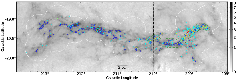
Figure 1: Greyscale: Meingast18 K-band extinction map. Yellow contours: Lane16 850 $\mu$m continuum image smoothed to 1′ resolution. The contour level is $\Sigma_{\rm mm}$ = 0.044 g cm^-2 (see §3.2). Blue contours: Meingast18 K-band extinction equivalent to $A_{V}=20$ mag. Cyan contours: Lane16 Getsources cores. White contour: Lane16 map coverage. Green polygon: The definition of ISF in Figure 10 (see §3.4). The red dashed ellipse shows the region that is masked for the detection probability study. The 1′ beam size is shown at the lower-left corner. The vertical dashed line splits the cloud into two regions with different level of feedback from massive stars. See §3.2.

We use the near infrared (NIR) extinction map of Orion A recently published by Meingast et al. (2018, hereafter Meingast18) to probe the cloud’s dust column density distribution at a resolution of 1′(or 2400 au), and a pixel scale of 30″ (see Figure 1). For our study, we mask the vicinity of the Orion KL region to avoid underestimated extinctions. We convert the map from $A_{K}$ to $A_{V}$ by multiplying by a factor of 8.93 (Rieke & Lebofsky, 1985). In the following, the extinction map is masked to have the same coverage as the continuum image.

2.3 Sub-mm Continuum Image and Core Catalog

We obtain the 850 $\mu$m continuum image from Lane et al. (2016, hereafter Lane16) for our study (publicly available at https://doi.org/10.11570/16.0008). The image was acquired as part of the JCMT Gould Belt Survey (Ward-Thompson et al., 2007; Salji et al., 2015; Mairs et al., 2016). The 850 $\mu$m map has a resolution of 14.6″ ($\sim$0.03 pc). Below we investigate the relation between continuum detection and cloud column density traced by the Meingast18 extinction map. First, we compare the continuum core catalog defined by Lane16 (the Getsources catalog) with the Meingast18 extinction map. Second, we carry out a pixel-by-pixel comparison between the Lane16 sub-mm continuum image and the Meingast18 extinction map without defining “cores”. Before the second comparison, we convolve the dust continuum image with a Gaussian kernel to have a final spatial resolution of 1′ and regrid it to the Meingast18 extinction map. The smoothed image has an rms noise of $\sigma_{850}$ = 10 mJy per 1′ beam.

Lane16 used an automask data reduction technique for the continuum image. This is a reduction strategy wherein astronomical flux (as opposed to atmospheric flux or noise) is identified automatically in the map-making procedure based on pixel SNR and the results of iteratively calculated noise models. For further details on the data reduction, see Chapin et al. (2013), Mairs et al. (2015), and Lane16. As a result, sources with sizes between 2.5′ and 7.5′ (0.3 pc and 0.9 pc at a distance of 400 pc) do not have robust flux measurements. Sources smaller than 2.5′ likely have robust flux measurements. Based on the work in Mairs et al. (2015), Lane16 indicated that strong, compact sources are well recovered, while faint, diffuse sources suffer more from flux loss. Since the goal is to target cores that are more centrally concentrated, i.e., more likely to develop protostars, we consider that the sub-mm continuum image satisfactorily represents the emerging cores in Orion A.

2.4 GAS Ammonia Core Catalog

We have obtained the NH₃ data from the GAS survey (Friesen et al., 2017; Kirk et al., 2017, hereafter Kirk17), which is publicly available at https://dataverse.harvard.edu/dataverse/GAS_DR1. Kirk17 selected a sample of cores from the larger sample of Lane16 based on the detection of NH₃ (observed with the Green Bank Telescope in the GAS survey, see Friesen et al., 2017) and studied their physical properties. In total, 237 continuum cores, most of them in the ISF, were included in their study. Kirk17 performed hyperfine line fitting to the NH₃ inversion lines and estimated the NH₃ core velocity $v_{\rm NH_{3}}$ and the kinetic temperature based on the ammonia emission. The GAS survey resolution is 32″, larger than some of the sub-mm cores in Lane16. Kirk17 (see their §3.2) have argued that the NH₃ traces the dense cores reasonably well. In this paper, we adopt the assumption that the dense core line-of-sight velocity is traced by the Kirk17 NH₃ line fitting result.

3 Results and Analyses

3.1 Sub-mm continuum detection

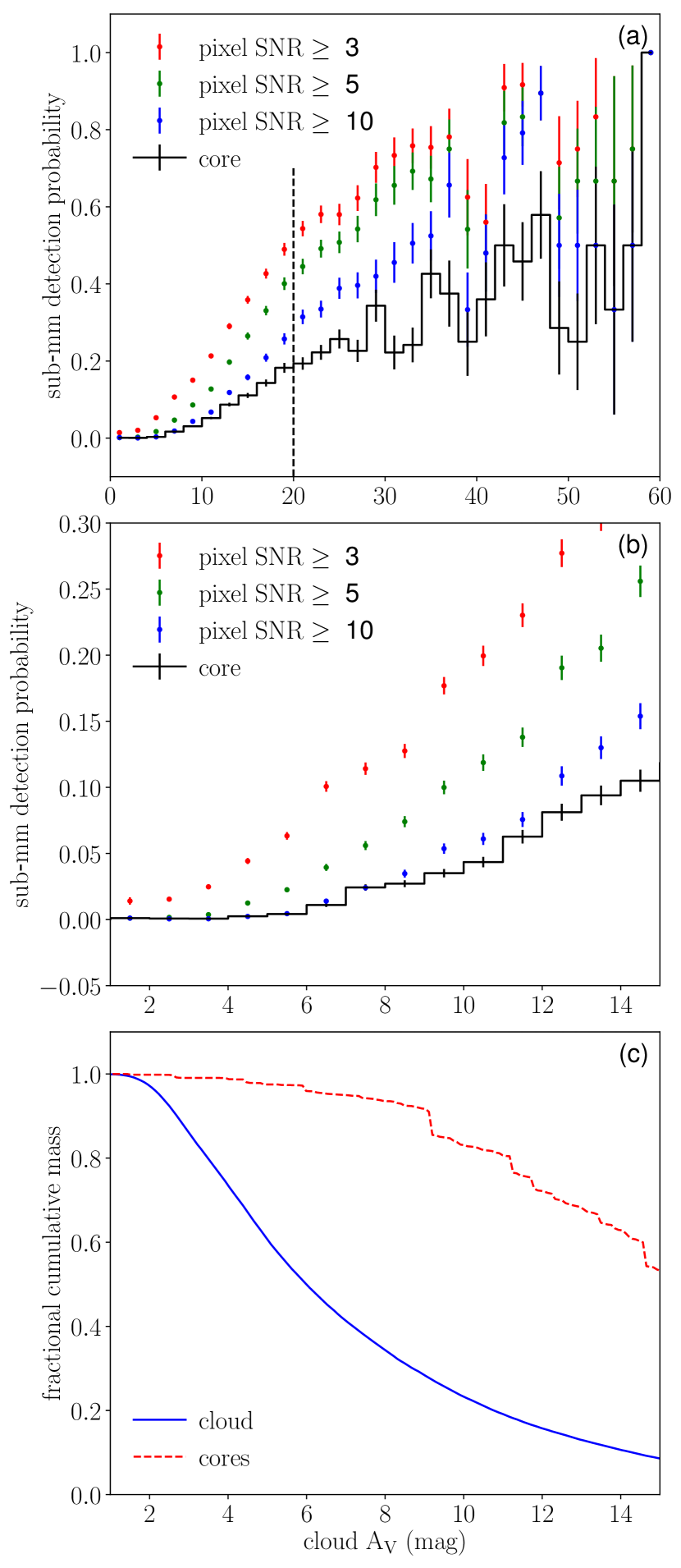
Figure 2: Continuum detection probability for Orion A. (a): The black histogram shows the core detection probability as a function of $A_{V}$. The color points are pixel detection probability functions. The continuum detection thresholds are indicated in the top-left legends. The vertical dashed line indicates the potential break. The bin size is 2 mag in $A_{V}$. (b): Same as panel (a), but zoomed in for $1<A_{V}<15$ mag. The bin size is 1 mag, compared to 2 mag for panel (a). (c): Cumulative distribution of extinction for the cloud (blue) and the cores (red). For each $A_{V}$, the distribution is the fraction of pixels/cores with extinction greater than $A_{V}$.

Figure 2(a) shows the continuum detection probability in Orion A. First, we investigate how likely the Lane16 cores are detected at a given $A_{V}$. We make $A_{V}$ bins every 2 mag. In each bin, the detection probability of the cores $P_{\rm c,850~{}\mu m}$ is defined as the number of pixels that contain cores ($N_{c}$) divided by the number of total pixels in the extinction bin $N_{\rm tot}$, i.e.,

$$P_{\rm c,850~{}\mu m}~{}=~{}N_{c}/N_{\rm tot}.$$ (1)

The error is estimated as

$$\sigma_{P}=[P_{\rm c,850~{}\mu m}(1-P_{\rm c,850~{}\mu m})/N_{\rm tot}]^{0.5}.$$ (2)

This estimation gives zero error when $P_{\rm c,850~{}\mu m}$ is 0 or 1 (see discussions in Kong et al., 2018a). Figure 2(b) zooms in to 1 mag $<A_{V}<$ 15 mag, with a bin size of 1 mag.

Figure 2(a) shows that the detection probability of the Lane16 continuum cores remains 0 for $A_{V}~{}\leq~{}5$ mag. At $A_{V}~{}>~{}5$ mag, the probability increases monotonically until $A_{V}~{}\sim~{}20$ mag, after which it has a shallower slope. In panel (b), the core detection (histogram) shows an increase after $A_{V}~{}\sim~{}7$ mag. Following Mairs et al. (2016, figure 7), we make a cumulative distribution function (CDF) for the cloud and core extinction, shown in the panel (c). The core CDF remains approximately flat until a turnover at $A_{V}\sim 9$ mag. Based on these, we assign a value to the core detection threshold in the range $A_{V}\sim 5-10$ mag. This is consistent with findings in Ophiuchus (9 mag, Young et al., 2006) and Perseus (5 mag, Enoch et al., 2006). As a massive star-forming cloud, Orion A does not show a significantly different extinction threshold of core formation compared to other lower-mass clouds. Moreover, these results are also consistent with Goldsmith et al. (2008); Lada et al. (2010); Heiderman et al. (2010) who investigated the SF extinction threshold using YSOs. The similarity between the core formation threshold and the SF threshold is not unexpected since stars form in dense cores. These comparisons potentially suggest a universal SF extinction threshold of $A_{V}=5-10$ mag in the clouds within 500 pc of the Sun.

It is also important to study continuum detections that are not identified as cores. They may be the precursors of cores as they become centrally peaked during fragmentation. We show in Figure 2(a)(b) the pixel-based 850 $\mu$m detection probability function (DPF). The pixel detection probability is the ratio between the number of extinction pixels that contain 850 $\mu$m dust emission detection and the number of total pixels within each extinction bin. Three continuum detection thresholds are applied, namely, SNR$\geq$3 (red); SNR$\geq$5 (green); SNR$\geq$10 (blue). The “detected” pixels defined this way may include noisy spikes in the image. Using a higher threshold can reduce a false detection at the expense of missing real emission.

As expected, the pixel-based continuum detection probability is larger than the core-based probability, since the cores are defined with a subset of detected pixels (Lane16). In fact, a notable number of the detected continuum pixels are not included in the cores defined by Lane16 Getsources catalog. As described in their appendix A.1.1, Lane16 set a threshold SNR = 7 for core detection. Further, they smoothed the 850 $\mu$m image and removed sources that did not appear significant, along with those rejected by the Getsources method. As a result, the number of “reliable” cores was reduced from 1178 to 919 (Lane16 final catalog). Figure 2 of Lane16 shows that only a fraction of the emission was grouped into cores.

As shown in Figure 2(a)(b), the DPF rises from 0 to close to 1 from $A_{V}=0$ mag to $A_{V}\sim 50$ mag. At a given extinction, only a fraction of the pixels are detected in continuum emission, caused by a combination of low temperature, spatial filtering effect, and/or opacity variation. At sub-mm and mm wavelengths, the flux density is approximately proportional to the column density and the temperature. The line-of-sight column temperature may have a major impact on the detection above a given threshold. The cores are likely heated by contraction and/or an embedded protostar (see also discussions in Kong et al., 2018a). Spatial filtering of large spatial structures helps in picking out centrally peaked dense cores. Meanwhile, the extinction traces the total column density. Therefore, we argue that the continuum detection pinpoints the forming dense cores embedded in the extinction column density.

The DPF thus shows that only a fraction of the cloud is forming stars at a given time, consistent with the theoretical expectation in, e.g., Krumholz & McKee (2005). An interesting feature in Figure 2(a) is the apparent break at $A_{V}\sim 20$ mag (vertical dashed line). For the DPF with SNR$\geq$10, a linear regression for $10\lesssim A_{V}\lesssim 20$ mag gives a slope of 0.024($\pm$0.001), while the slope for $20\lesssim A_{V}\lesssim 30$ mag is 0.012($\pm$0.001). Interestingly, $A_{V}=20$ mag is also where the core detection slope becomes shallower. For reference, Figure 1 shows the regions with $A_{V}=20$ mag with blue contours. It remains to be seen if the 20 mag break is detected in other clouds.

The total mass of the Lane16 cores is $\sim$ 1400 M_⊙. We follow Lane16 equation (1) for the mass calculation. This was also adopted by Kirk17. Note this number has been scaled down by a factor of 0.8 compared to the Lane16 and Kirk17 core mass because we use 400 pc as the cloud distance while they used 450 pc. The total cloud mass converted from the Meingast18 extinction map is $\sim$ 36,000 M_⊙ within the Lane16 mapped area. The Lane16 core mass fraction is therefore $\sim$ 4.0% of the mass estimated from the extinction map. If we include all Lane16 sub-mm continuum flux above a SNR of 5, the mass fraction increases to $\sim$ 14%.

3.2 Comparison with IRDC G28.37+0.07

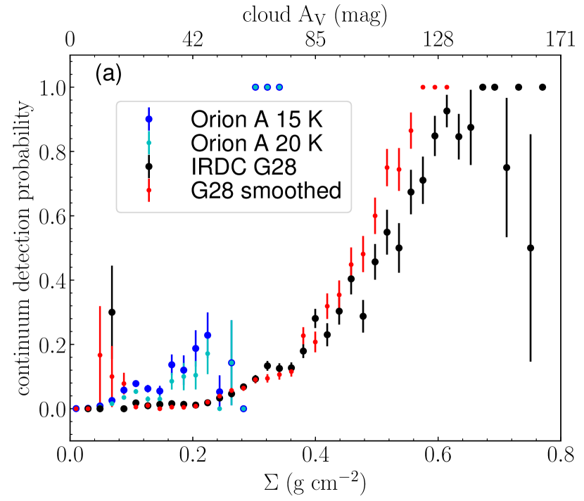
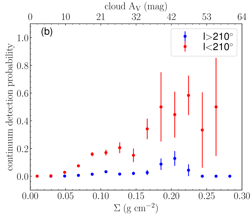
Figure 3: (a): Continuum pixel detection probability for Orion A (blue) and IRDC G28 (black). The red points are from smoothed G28 data that matches the physical resolution of the Orion A data. The cyan points are the same as the blue ones except that we use 20 K to calculate the detection flux threshold. See §3.2. (b): Continuum pixel detection probability for two sub-regions in Orion A (divided at l=210°, indicated by the vertical dashed line in Figure 1).

To investigate the dense gas emergence in different environments, we compare the Orion A DPF with the DPF from the infrared dark cloud (IRDC) G28.37+0.07 (hereafter G28). Kong et al. (2018a) studied the DPF in IRDC G28 with ALMA 1.3 mm continuum data. Although the DPF in Orion A is derived with 850 $\mu$m continuum, the comparison is still meaningful once we apply the same physical threshold. For comparison, the physical resolution is 0.05 pc in the IRDC G28 study (Kong et al., 2018a). The maximum detectable scale was 0.5 pc. In IRDC G28, assuming a temperature of 15 K and volume density of 10⁵ cm^-3, the Jeans length is $\sim$ 0.1 pc. We also smooth the G28 data to a resolution of 0.12 pc, in order to match the linear resolution of the IRDC data with that of the Orion A study. The fiducial 1.3 mm continuum detection threshold in mass surface density was set to $\Sigma_{\rm mm}$ = 0.044 g cm^-2 in Kong et al. (2018a). To match this number in Orion A, we compute the mass surface density following equation (1) in Lane16 and adopting the same assumptions of dust temperature and opacity. The threshold is shown as the yellow contours in Figure 1.

Figure 3(a) shows the comparison of DPFs between Orion A and IRDC G28. We use the same bin size of 0.02 g cm^-2 for both clouds, following Kong et al. (2018a). Note that this number is converted from extinction (hereafter denoted $\Sigma_{\rm ex}$), which is different from the sub-mm continuum detection threshold (also in g cm^-2, but from emission). The highest extinction traced by the Meingast18 map is about 0.3 g cm^-2. Recently, Stutz (2018) used Herschel far infrared and APEX 870 $\mu$m data to derive a column density map in Orion A. The highest surface density reaches $\sim$ 3 g cm^-2 in the Orion KL region. The near infrared extinction does not work well in this region. However, the number of pixels in this region only accounts for $\sim$0.1% of the Lane16 coverage. We ignore these pixels by removing them from the comparison (red dashed ellipse in Figure 1).

As shown in Figure 3(a), the Orion A cloud shows more continuum detection of dense gas with $\Sigma_{\rm mm}\geq$ 0.044 g cm^-2 than IRDC G28. The difference appears within 0.08 $\lesssim\Sigma_{\rm ex}\lesssim$ 0.28 g cm^-2. For this we followed Lane16 and Kirk17 and assumes dust temperature of 15 K. Kong et al. (2018a) assumed 20 K for their dust continuum emission because they argued that the cores were mostly protostellar. For consistency, we also calculate a new DPF assuming a dust temperature of 20 K in Orion A (cyan dots in Figure 3(a)). A higher dust temperature requires a higher continuum flux to reach the same mass surface density threshold of 0.044 g cm^-2, therefore the cyan detection probability becomes lower. Nonetheless, the Orion A DPF is still higher than the G28 DPF within 0.08 $\lesssim\Sigma_{\rm ex}\lesssim$ 0.28 g cm^-2. A two-sample KS test gives a KS statistic of 0.8 with a p-value of 0.0012, meaning the null hypothesis that the two samples are drawn from the same distribution can be rejected at a significance level below 1% (confidence over 99%).

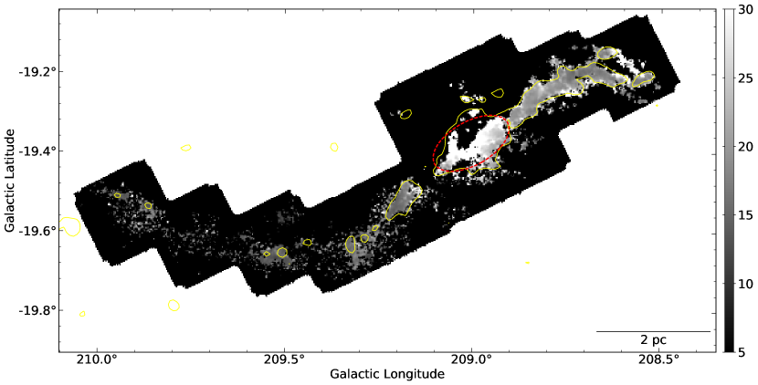
Figure 4: Kirk17 NH₃ gas kinetic temperature map. The color bar ranges linearly from 5 K to 30 K. The yellow contours and the red ellipse are the same as in Figure 1.

The main source of uncertainty is likely the temperature assumption. For a given mass, a higher dust temperature indicates a higher continuum flux. Therefore, we need to set a higher flux threshold for the same mass threshold. This gives rise to lower detection probability, which is illustrated by the blue and cyan points in Figure 3(a). Lane16 pointed out that the high dust temperature from Herschel results (Lombardi et al., 2014) likely trace the dust in lower density regions along the line-of-sight and thus underestimate the core mass. In Figure 4, we show the Kirk17 NH₃ kinetic temperature map. Again, the yellow contours show the regions with a continuum surface density equal to or greater than 0.044 g cm^-2. The regions enclosed by the yellow contours in Figure 3 are dominated by temperatures below 20 K.

The effect of spatial filtering may be important when comparing the DPF in both clouds. Both the ALMA data and the JCMT data filter out emission from structures at large spatial scales. Therefore, the continuum emission in both maps detect relatively compact structures, that presumably trace the dense gas intimately involved in the core formation process. In the JCMT 850 $\mu$m image, structures larger than 2.5′ (0.3 pc) are not robustly recovered. In the ALMA 1.3 mm image, the maximum sensible scale is 12″ (0.3 pc, which is 0.6 times the maximum scale that corresponds to the shortest baseline, see Kong et al., 2018a). Therefore, we argue that both DPFs are tracing similar dense structures, and Orion A is more capable of forming dense gas/cores than the IRDC G28.

One significant difference between G28 and Orion A is that the former is likely forming the very first generation of stars in the mapped region. In particular, the area studied by Kong et al. (2018a) is mostly dark up to 70 $\mu$m. As opposed to Orion A, there is no feedback (radiation, spherical wind/bubble) from massive stars in IRDC G28, although massive stars may eventually form there (Zhang et al., 2015; Kong et al., 2018b).

To test if the high DPF in Orion A is related to feedback, we split the Orion A map in two, indicated by the vertical dashed line along l=210° in Figure 1. The region on the east side (l$>$210°) is less influenced by feedback from the Trapezium cluster compared to the region on the west side (l$<$210°, Bally, 2008). As shown in Figure 3(b), the high sub-mm continuum detection probability in Orion A is dominated by the l$<$210°sub-region, suggesting that strong feedback may indeed result in higher values in the DPF for the same cloud extinction (see §4.1).

3.3 Core-to-envelope velocity

We investigate the relative motion between the dense cores traced by NH₃ (§2.4) and the ambient cloud traced by CO isotopologues (§2.1). Similar studies include Walsh et al. (2004) and Kirk et al. (2010). We first convolve the CARMA-NRO cubes to 32″ angular resolution to match the GAS data. Then, for each core we extract a spectrum averaged over the 32″ circular area centered on the Kirk17 core position. We fit a Gaussian to the spectra in order to derive the bulk gas velocity component (1D) along the line of sight, with the optically thin assumption. In fact, we have shown in K18 that more than 99% of the ¹³CO pixels have $\tau<$1 (see their §5.2). The maximum core optical depth for the ¹³CO(1-0) line is 1.12 and 98% of the cores have optical depth $<$ 1.

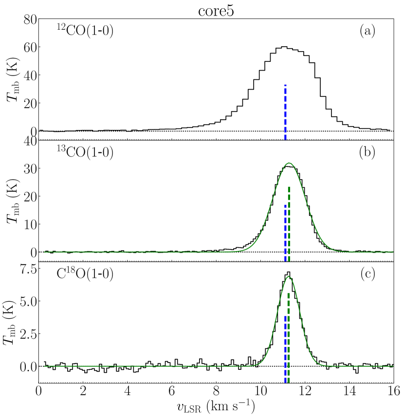
Figure 5: ¹²CO(1-0) (top), ¹³CO(1-0) (middle), and C¹⁸O(1-0) (bottom) spectra for core 5 in Kirk17. The baselines are shown as the black horizontal dashed lines. The blue vertical dashed lines indicate $v_{\rm NH_{3}}$. The green curves show the Gaussian fit to the spectra (only for ¹³CO and C¹⁸O), with the green vertical dashed lines showing the centroid velocities $v_{\rm gauss}$.

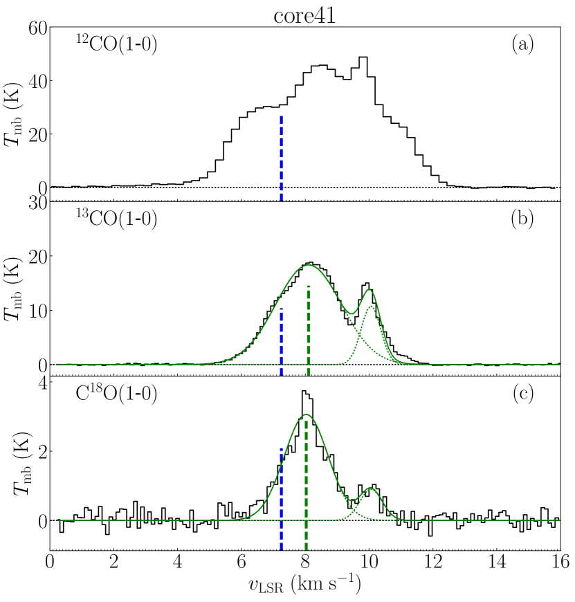
Figure 6: Same as Figure 5, but for core 41. The green dashed line shows the centroid velocity $v_{\rm gauss}$ of the Gaussian component that is closest to $v_{\rm NH_{3}}$. The green dotted curves show the fitting to each Gaussian component.

Figure 5 shows the spectra of core number 5 in the Kirk17 sample. We show the spectra of ¹²CO(1-0), ¹³CO(1-0), and C¹⁸O(1-0) in black. In order to perform the Gaussian fit, we visually identify the number of Gaussian components for each spectrum and provide the initial guess for amplitude, centroid velocity, and velocity dispersion for each spectrum. Then, we use the scipy.optimize.curve_fit function from the python package Scipy to perform single-/multi-Gaussian fitting to ¹³CO and C¹⁸O spectra. If there is only one component, we take the centroid velocity $v_{\rm gauss}$ as the envelope velocity. If more than one velocity component is identified, we take the one that is nearest to $v_{\rm NH_{3}}$ as the envelope velocity, similar to the study by Kirk et al. (2007, see their discussions in section 5 and figure 6).

Core 5 (Figure 5) shows one Gaussian component in ¹³CO and C¹⁸O spectra. However, a significant fraction of the cores show complex velocity features. In Figure 6, we show another example, core 41. This core has roughly three velocity components in the ¹²CO(1-0) line and two components in ¹³CO(1-0) and C¹⁸O(1-0). $v_{\rm NH_{3}}$ of this core does not corresponds to any of the carbon monoxide line components. Based on our visual identification, 100 out of the 237 cores from Kirk17 show multiple velocity components in either the ¹³CO or the C¹⁸O spectrum (or both). ¹²CO spectra typically show more complex profiles.

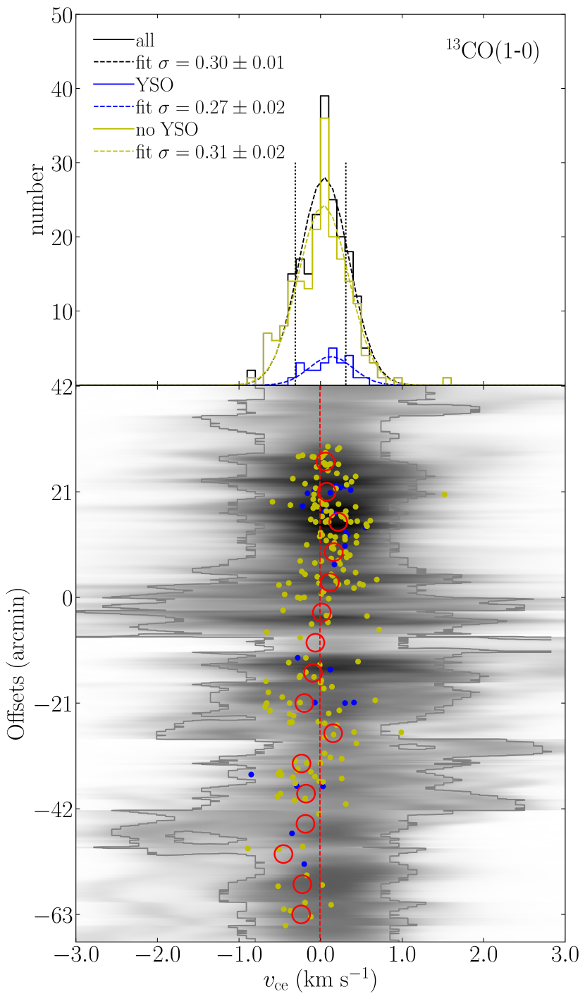
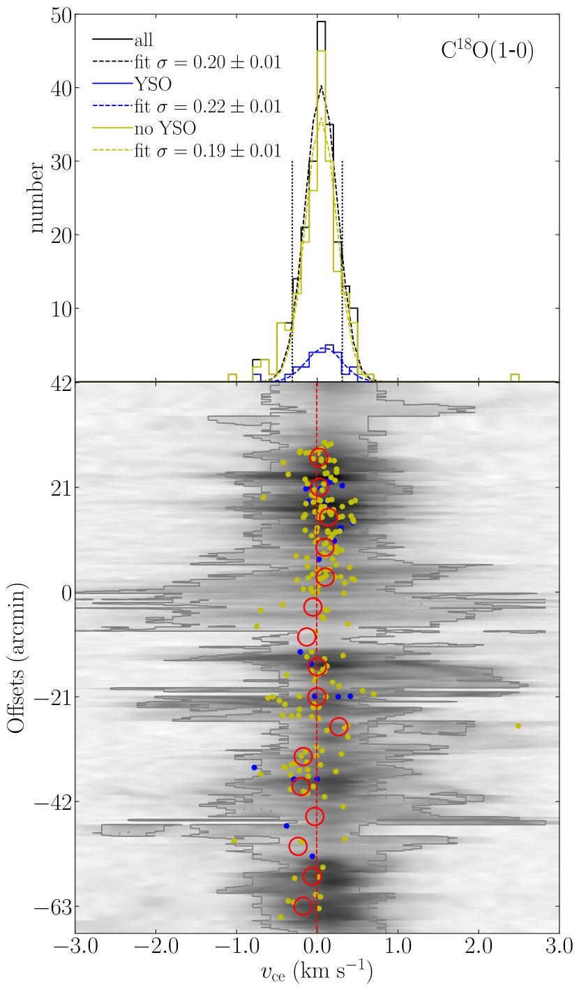
Figure 7: Left: Top panel: Histograms of core-to-envelope velocity differences $v_{\rm ce}$(¹³CO). The black histogram shows the distribution for the entire Kirk17 core sample. The black dashed curve shows the Gaussian fit to the black histogram. The blue histogram and dashed curve correspond to the cores with YSO; the yellow without YSO. The dispersion values obtained from Gaussian fits to the histograms are shown in the upper left corner. The vertical dotted lines show the sound speed. Bottom panel: The gray background shows the PV-diagram along the orange curve in Figure 10. The zero offset is the big red dot on the orange curve between OMC-1 and ONC. Positive offset is toward the north (OMC-2/3 direction). Note that 21 arcmin corresponds to $\sim$2.5 pc at 400 pc. At each offset, the PV-diagram zero velocity is defined at the intensity peak. The gray contour denotes the half maximum at each offset. The yellow dots denote the starless cores and the blue dots denote the cores with YSO. The offset (y-axis) is along the ISF spine (orange curve). The empty red circles are offset bins every 6′. Their $v_{\rm ce}$ values are averaged within the bins. Right: Same as left, but for $v_{\rm ce}$(C¹⁸O).

To estimate possible systematic difference between the dense core velocity $v_{\rm NH_{3}}$ and the envelope gas velocity, we calculate for each core the 1D core-to-envelope velocity $v_{\rm ce}\equiv v_{\rm NH_{3}}$ - $v_{\rm gauss}$ using the ¹³CO(1-0) and C¹⁸O(1-0) line Gaussian fitting results. In the top panels of Figure 7, we show the distributions of $v_{\rm ce}$(¹³CO) and $v_{\rm ce}$(C¹⁸O) (black bins), respectively. The bin size is 0.1 km s^-1. We then fit a Gaussian to the $v_{\rm ce}$ distribution. We can see the 1D core-to-envelope Gaussian dispersion $\sigma_{\rm ce}$ is 0.20$\pm$0.01 km s^-1 for C¹⁸O and 0.30$\pm$0.01 km s^-1 for ¹³CO. We also apply the maximum likelihood method (using scipy.stats.norm.fit) to estimate $\sigma_{\rm ce}$, which gives $\sigma_{\rm ce}$(¹³CO) = 0.33 km s^-1 and $\sigma_{\rm ce}$(C¹⁸O) = 0.25 km s^-1 (removing the outlier beyond 2 km s^-1; if not, $\sigma_{\rm ce}$ = 0.30 km s^-1).

We investigate the effect of varying envelope sizes by extracting envelope spectra from a number of circular regions centered on the core but with different radii. For this purpose we use the original CARMA-NRO Orion Survey data cubes (i.e., before smoothing to 32″ resolution). At each core location, we extract ¹³CO and C¹⁸O spectra from circular regions with diameters 8″, 16″, 32″, 64″, and 128″, i.e., factors of 2 increase from the beam size (8″ corresponds to a physical scale of 0.015 pc). The respective fitting results of the core-to-envelope dispersion for ¹³CO are 0.29 km s^-1, 0.30 km s^-1, 0.30 km s^-1, 0.34 km s^-1, 0.39 km s^-1; for C¹⁸O they are 0.26 km s^-1, 0.25 km s^-1, 0.25 km s^-1, 0.26 km s^-1, 0.32 km s^-1. As we compare the core velocity to that of the envelopes averaged over a larger area, the velocity dispersion becomes slightly higher.

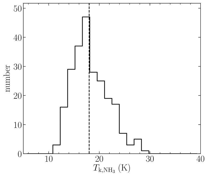
Figure 8: Histogram of core kinetic temperature derived from NH₃ inversion lines. The data are taken from Kirk17. The vertical dashed line shows the median temperature (18 K) used to compute the sound speed.

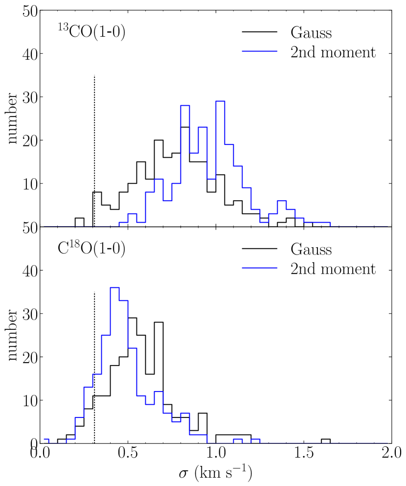
Figure 9: Histograms showing the distribution of the line dispersion in the ¹³CO (top panel) and C¹⁸O (bottom panel) spectra from cores. The black histograms show the distribution of dispersion values obtained from gaussian fits to the spectra, while the blue histograms show the distribution of values obtained from the second moment of the spectra. The vertical dotted line shows the sound speed calculated at 18 K.

In the top panels of Figure 7 we indicate the sound speed, calculated using a gas temperature of 18 K (following appendix A1 in Orkisz et al., 2017), by the vertical dotted lines. Figure 8 shows the distribution of core gas kinetic temperatures derived from NH₃ data (Kirk17). The mean temperatures are 18.3 and 17.8 K, respectively, while the minimum and maximum temperature are 11.3 and 29.3 K, respectively We adopt 18 K as the representative temperature for the sound speed calculation (which results in a value of 0.31 km s^-1). For C¹⁸O, the sound speed is at 1.55$\sigma_{\rm ce}$, which from the Gaussian fitting to $v_{\rm ce}$(C¹⁸O) would imply that about 88% of the cores have relative motion slower than the local sound speed (note that from the data, the actual fraction of cores with $v_{\rm ce}$(C¹⁸O) $<$ 0.31 km s^-1 is 78%.) For ¹³CO, the sound speed is at 1.0$\sigma_{\rm ce}$. Based on the Gaussian fitting, this implies that 68% of the cores have relative motion slower than the local sound speed (the actual fraction of cores with $v_{\rm ce}$(¹³CO) $<$ 0.31 km s^-1 is 66%). Note that the velocity dispersion and sound speed discussed here are both 1D quantities.

Figure 9 shows the distribution of line velocity dispersions for ¹³CO(1-0) and C¹⁸O(1-0) (black bins). Again, we indicate the sound speed as the vertical dotted line. The figure shows that the majority of cores are located in regions where the carbon monoxide gas line dispersion is supersonic. Therefore, the core-to-envelope velocity dispersion $\sigma_{\rm ce}$ is significantly smaller than the local line width. In the bottom panels of Figure 7, we show the core-to-envelope velocities on top of the PV-diagram along the ISF ridge defined in K18 and Figure 10. As can be seen, for the vast majority of cores, the core-to-envelope velocities $v_{\rm ce}$(¹³CO) and $v_{\rm ce}$(C¹⁸O) are predominantly smaller than the velocity FWHM at the position of the core (shown as gray contours in Figure 7), confirming the results from the Gaussian fittings. Through a study of the kinematics in the Orion Nebula Cluster (ONC), Tobin et al. (2009) showed that the stars and ¹³CO gas are kinematically tied, consistent with our results for dense cores.

We made separate histograms of $\sigma_{\rm ce}$ for cores with and without YSOs in order to investigate whether there is a difference between pre- and protostellar cores as a result of evolution. The YSO-core assignment is given by Lane16, where they checked against catalogs from Megeath et al. (2012, Spitzer observation) and Stutz et al. (2013, Herschel observation). In Figure 7, we show $v_{\rm ce}$ distribution for protostellar cores as blue histograms; starless cores as yellow histograms. The $v_{\rm ce}$ dispersions between the two populations are different by 10%. The $v_{\rm ce}$ centroid for the starless cores is 0.03$\pm$0.02 km s^-1 in the ¹³CO fitting; for the protostellar cores 0.13$\pm$0.02 km s^-1. In the C¹⁸O fitting, the $v_{\rm ce}$ centroid for the starless cores is 0.04$\pm$0.01 km s^-1; for the protostellar cores 0.08$\pm$0.01 km s^-1. The cores with YSOs tend to have an excess of positive core-to-envelope velocities. However, note the limited number of cores with associated YSOs (see the blue dots in Figure 7).

3.4 Filament and core dynamics

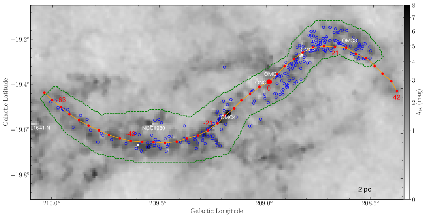
Figure 10: Cores on the Integral-Shaped Filament in Orion A. The gray-scale background image shows the extinction map from Meingast et al. (2018). The blue circles mark the position of the Kirk17 cores. The green dashed contour shows the filament defined for estimating $m_{l}$ in §3.4. The orange curve defines the PV cut following figure 5 of Kong et al. (2018c) but extending further to cover the entire core sample in the east. The red dots along the curve indicate 3′ segments. The red numbers show the offsets in Figure 11.

We re-analyze the filament virial status in the context of the model by Fiege & Pudritz (2000). In this model, the virial velocity for an unmagnetized filamentary cloud is related to the mass per unit length $m_{l}$ by:

$$\sigma_{\rm vir}=\sqrt[]{\frac{Gm_{l}}{2}},$$ (3)

where G is the gravitational constant.

Fiege & Pudritz (2000) used the Orion A ¹³CO data with a resolution of 1.7′ from Bally et al. (1987) to derive a value of $m_{l}=355$ M_⊙ pc^-1 for the ISF. We use the extinction map (Meingast et al., 2018) to estimate the ISF mass. Figure 10 shows our definition of the filamentary region. We define the entire ISF filament region to roughly cover the Kirk17 core sample (green dashed polygon). The total mass of the filament is $\sim$3835 M_⊙ and the total length is $\sim$12 pc. The length is derived from a visually-defined curve that follows the ridge line of the ISF (originally defined in figure 5 of K18, but extended to the eastern end of the filament). The recent GAIA data show that the ISF is likely parallel to the plane of the sky (Großschedl et al., 2018), although with a few pc variation (Stutz et al., 2018). Hence, we do not correct the length of the filament due to inclination effects. The ISF $m_{l}$ we derive is 320 M_⊙ pc^-1, a factor of 0.90 smaller than Fiege & Pudritz (2000). This falls in the $m_{l}$ range (125-800 M_⊙ pc^-1) estimated by Stutz & Gould (2016, see their figure 5). Our estimated virial velocity for an unmagnetized filament is $\sigma_{\rm vir}\sim$0.83 km s^-1.

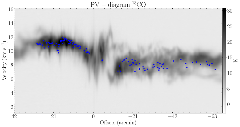
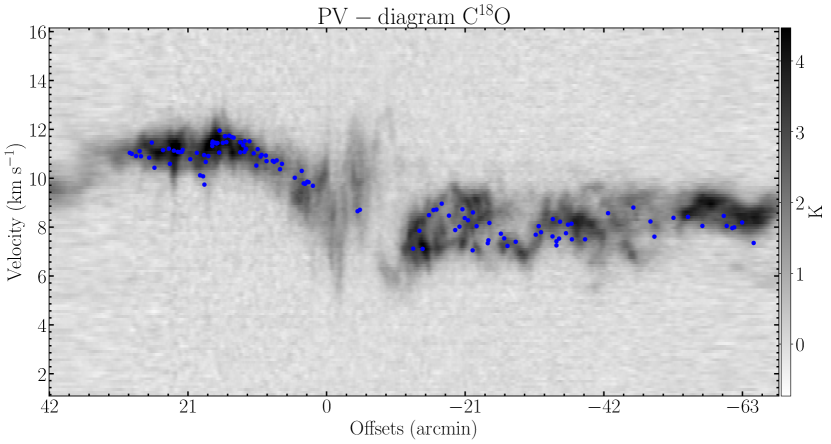
Figure 11: Position-velocity (PV) diagrams along the ISF using the ¹³CO (top) and C¹⁸O (bottom) data. The PV cut is defined as the orange curve along the ISF spine with a width of 3′(Figure 10). The zero-offset position is the large red dot between OMC1 and ONC in Figure 10. The positive offset is toward the west direction (OMC-2/3). Note that 21 arcmin corresponds to $\sim$2.5 pc at 400 pc. The blue dots show the Kirk17 cores. The velocity is different from Figure 7 bottom panels where the zero velocity is the gas intensity peak.

Recall from §3.3 that the core-to-envelope velocity dispersion $\sigma_{\rm ce}$ for ¹³CO and C¹⁸O is 0.30 and 0.20 km s^-1, respectively. Applying a factor of $\sqrt[]{3}$, the 3D dispersion for ¹³CO is 0.52 km s^-1 and for C¹⁸O is 0.35 km s^-1. Both numbers are smaller than the $\sigma_{\rm vir}$ in the unmagnetized scenario, indicating that the cores are bound to the ISF filament. In the presence of magnetic fields, $\sigma_{\rm vir}$ depends on both the poloidal field in the filament and the helical field that wraps the filament. More robust measurements of the field strength are needed (note the recent progress by Pattle et al., 2017; Tahani et al., 2018).

Note that the ISF has an overall velocity gradient and the core kinematics follow the trend. To illustrate this, we make PV-diagrams along the ISF for ¹³CO and C¹⁸O, shown in Figure 11. The PV-cut follows the orange curve from Figure 10. The offsets in Figure 11 are labeled as the red numbers in Figure 10. We also overplot the cores on the PV-diagram. As one can see, the ISF shows a wave-like velocity structure (see K18 figures 20-22; also see Stutz & Gould, 2016) and the cores closely follow the ISF kinematics. The overall velocity distribution of the ISF results in a super-virial core-to-core velocity dispersion of 2.92 km s^-1, which is different from what was seen in Perseus (sub-virial core-to-core dispersion, Kirk et al., 2010; Foster et al., 2015). While the final fraction of gas in Orion A and Perseus that is deposited into stars (SF efficiency) is unclear, the forthcoming star cluster in Orion A is less likely to be bound compared to the cluster in Perseus. This emphasizes the importance of the initial condition for star cluster formation.

4 Discussion

4.1 Comparing core formation capability between Orion A and IRDC G28

Within the range 0.08 $\lesssim\Sigma_{\rm ex}\lesssim$ 0.28 g cm^-2, Orion A appears to be more capable of forming dense cores than G28 (Figure 3). In §3.2 we suggested that this could be caused by SF feedback in Orion A, although we did not indicate the main feedback mechanism that could be responsible for this. Outflows are unlikely the source for the difference between Orion A and G28, as both clouds have widespread outflows (Davis et al., 2009; Bally et al., 2017; Kong et al., 2019). The main difference likely comes from the presence of massive star feedback in Orion A (the region of G28 studied in Kong et al. (2019) is not impacted by massive stars). In Figure 4 we have shown that the dense gas in Orion A is not significantly heated, thus the heating from ionizing photons is not likely dominating the difference between these two clouds. We suggest that pressure from the expanding HII region (Pabst et al., 2019), which possibly compresses the cloud and generates more dense gas, may be responsible for the higher incidence of dense cores in Orion A. Feddersen et al. (2018) reported expanding shells and bubbles in Orion A, which may also be important in generating dense gas. Our results emphasize the important role of stellar feedback in SF.

4.2 ISF core group dynamics

The sub-sonic core-to-envelope kinematic feature we detect in Orion A is seen in other nearby star-forming clouds (i.e., Taurus, Perseus, Ophiuchus, see Walsh et al., 2004; Kirk et al., 2007, 2010; Foster et al., 2015), although the Orion A cloud is quite different from these clouds in terms of active massive SF and destructive feedback. These suggest that dense molecular cores remain tied to their host clouds during their formation regardless of the environment.

The kinematics of cores can be useful in testing SF theories. For instance, in the competitive accretion model (Bonnell et al., 2001; Smith et al., 2009), protostars and the host cloud globally collapse toward the cloud’s gravitational potential minimum. As shown by Bonnell et al. (2001), protostars compete for the gas through tidal accretion and the relative velocity between a protostar and the surrounding gas is sub-sonic throughout the global collapse. However, it is to be clarified how the cores seen in observations are linked to the structures seen in the simulations. For instance, detailed radiative transfer modeling may be necessary to show if the tidal sphere in simulations corresponds to the dense cores in observation. On the other hand, the fact that dense cores have low core-to-envelope velocity dispersion is a fundamental prediction of the “colliding flow” model in Padoan et al. (2001). Cores do not move freely in the envelope because they form in the post-shock gas at the intersection of colliding flows (i.e., in regions where the flow velocity stagnates, as it is dissipated in shocks).

4.3 The dynamical status of the ISF

The work by Tobin et al. (2009) have shown the similarity in the kinematics between the stars and ¹³CO gas in the ISF. Subsequently, Hacar et al. (2016); Stutz & Gould (2016); Getman et al. (2019) explored the kinematic link between YSOs and the cloud gas in Orion A. Together with our findings, these results suggest that SF is ongoing in the ISF and that the low velocity dispersion in the protostars relative to their local gas probably originates from the low core-to-envelope velocity reported here. However, the explanation of the origin and the future of the ISF remains unclear, and various hypotheses have been proposed.

Tobin et al. (2009) argued that the ISF cloud and stars are undergoing a global collapse toward the ONC. The basis for their argument was the observed velocity gradient along the declination direction. The gas kinematics and the radial velocity of the young stars show a change toward red-shifted velocities in the OMC-2/3 regions north of the ONC (their figure 3), while the southern ISF shows an approximately flat velocity distribution. Tobin et al. (2009) thus argued that the ISF is collapsing toward the ONC, with the OMC-2/3 regions located on the near side but having red-shifted velocities.

With a higher resolution (30″) N₂H⁺ data, Hacar et al. (2017) revisited the topic. They also argued that the ISF is undergoing gravitational collapse toward the ONC. However, their picture supports a collapse from the far side. The basis for their argument is the blue-shifted velocity gradients in both the north and south of the cluster (see their Figure 1c) combined with the inference that the ONC must be on the near side of the ISF. Note that the collapse scale in Hacar et al. (2017) is smaller than that discussed in Tobin et al. (2009).

Recent analyses with APOGEE and Gaia surveys have shown that the ONC is slowly expanding (Kounkel et al., 2018; Kuhn et al., 2019), raising the question that whether gas is falling into ONC. However, it is possible if the ISF collapsing direction is toward OMC-1 (the densest gas region in the ISF), as Getman et al. (2019) recently have suggested that the stars in the OMC-1 region are undergoing gravitational contraction. On the other hand, Getman et al. (2019) showed that OMC-4/5 are not moving toward OMC-1. This raises the question whether the ONC/OMC-1 region is the gravitational focus. Meanwhile, it is possible that the global collapse is strongly impacted by the intense feedback in the area, resulting in a very complex environment.

Alternatively, Stutz & Gould (2016) and Stutz (2018) proposed the “slingshot mechanism” for the formation of stars in ISF of Orion A. They emphasized the wave-like geometry of the ISF and postulated that the filament has an oscillatory motion. In this scenario, cores move with the filament and the newly-formed stars are ejected from the oscillating filament once they are massive enough to decouple from the dense gas. The model addressed the wave-like spatial and kinematic morphology of the ISF and provided another explanation of the high velocity of newly-formed stars. Recently, Stutz et al. (2018) used Gaia data to suggest that the ISF filament is a standing wave.

With our newly acquired CARMA-NRO Orion gas data, but making the PV-diagram along the ISF (instead of declination, see Figure 10), we detect more complicated kinematic features (Figure 11). The cloud shows a “wave-like” feature (more so in the north with positive offsets in Figure 11 than in the south). Such kinematics present a challenge in terms of simply explaining the ISF with a global collapse toward ONC. Moreover, the northern part shows an oscillatory feature at scales of $\sim$ 3′. All these results suggest rather complex cloud kinematics and more information is needed to understand the origin and evolution of the ISF.

We notice something interesting from the core-to-envelope PV-diagrams in Figure 7. In the bottom panels, we bin the core-to-envelope velocities along the ISF. Each empty red circle represents the average core-to-envelope velocity within a 6′ bin. Along the ISF, the distribution of the red circles is again oscillatory. Note that this is not the wave-like structure of the filament gas. As shown in the figures, the cores are red-shifted relative to the gas in the OMC-2/3 regions (positive offsets), while in the southern region (negative offsets) the cores are blue-shifted relative to the gas. The origin of the core motion is unclear, and this is the first time they are detected. It is not clear why one should expect an oscillatory motion in velocities between the core and the gas, but it does remind us of the slingshot mechanism because of the “wave”. The expanding bubble from the Trapezium cluster may push away low-density envelopes (Pabst et al., 2019), resulting in an apparent shift of the core-to-envelope velocity. However, this scenario would require the impact of the feedback at very high extinctions and far away from the location of massive stars along the entire ISF (see discussions in Großschedl et al., 2018), as the cores are deeply embedded.

5 Conclusions

In this paper, we studied sub-mm continuum core formation and kinematics in the Orion A molecular cloud. Various sources of publicly available and proprietary data were combined with our CARMA-NRO Orion Survey data for the study. Below we list our major conclusions.

1. We have compared 850 $\mu$m continuum core detections (Lane et al., 2016) with NIR extinction (Meingast et al., 2018). We find a detection threshold of $A_{V}\approx$ 5-10 mag for the cores within the declination range of (-9.5°, -4.5°). Together with previous findings in Ophiuchus and Perseus, we suggest a universal core formation extinction threshold of $A_{V}\sim$ 5-10 mag for clouds within 500 pc from the Sun. This threshold also appears to be consistent with the star formation extinction threshold suggested by Goldsmith et al. (2008); Lada et al. (2010); Heiderman et al. (2010). The total 850 $\mu$m core mass is about 4% of the mass of the entire Orion A cloud.

2. A pixel-by-pixel comparison between the sub-mm continuum and the NIR extinction shows a steady increase in the continuum detection probability for $A_{V}$ between $\sim$ 5 and 20 mag, and a potential turning point at $A_{V}\sim$20 mag where the slope in the relation decreases. This turning point is also seen in continuum core detection.

3. We have compared the pixel-based continuum detection in Orion A with the infrared dark cloud G28.37+0.07. Within the cloud extinction range of 15 mag $\lesssim A_{V}\lesssim$ 60 mag, Orion A shows more dust continuum emission detection, suggesting Orion A has been able to form more dense gas ($\Sigma_{\rm mm}\gtrsim$ 0.044 g cm^-2). Our study shows that the feedback from high-mass stars in Orion A, possibly expanding HII regions, is a potential cause of the difference between these two clouds. The continuum detection probability function (DPF) can be useful in showing the differences in core formation between clouds.

4. We have investigated the dense core kinematics within the Orion A integral-shaped filament (ISF). In particular, we compare the velocities of the dense cores (traced by NH₃) with the velocity of their surrounding lower density envelope (traced by ¹³CO and C¹⁸O). We find that the 1D dispersions in the distribution of the core-to-envelope velocity are 0.20 and 0.30 km s^-1, when using C¹⁸O and ¹³CO to trace the envelope, respectively. These are comparable to the sound speed of the dense gas and smaller than the local line dispersion in the ¹³CO(1-0) and C¹⁸O(1-0) spectra. This is consistent with previous findings in Perseus, suggesting that the dense molecular cores are kinematically tied to their parent cloud, independent of the cloud environment. However, compared to Perseus, the ISF core-to-core velocity dispersion is super-virial, largely due to the overall velocity gradient in the ISF. This difference may impact the dynamics of the forthcoming cluster in the future, which emphasizes the importance of initial cloud conditions for star cluster formation.

5. The cloud gas velocity and the core-to-envelope velocity both show wave-like features in PV-diagrams, although the two are conceptually different. Their relation to the overall dynamical picture of the ISF is to be determined, but see Stutz (2018) for recent work addressing the wave-like signature in the ISF. The kinematic difference between the dense cores and the cloud presented in this work remains to be theoretically addressed.

References

- Astropy Collaboration et al. (2013) Astropy Collaboration, Robitaille, T. P., Tollerud, E. J., et al. 2013, A&A, 558, A33
- Bally (2008) Bally, J. 2008, Overview of the Orion Complex, ed. B. Reipurth, 459
- Bally et al. (2017) Bally, J., Ginsburg, A., Arce, H., et al. 2017, ApJ, 837, 60
- Bally et al. (1987) Bally, J., Langer, W. D., Stark, A. A., & Wilson, R. W. 1987, ApJ, 312, L45
- Bonnell et al. (2001) Bonnell, I. A., Bate, M. R., Clarke, C. J., & Pringle, J. E. 2001, MNRAS, 323, 785
- Brown et al. (2018) Brown, A. G. A., Vallenari, A., Prusti, T., et al. 2018, A&A, 616, A1
- Chapin et al. (2013) Chapin, E. L., Berry, D. S., Gibb, A. G., et al. 2013, MNRAS, 430, 2545
- Clark & Glover (2014) Clark, P. C., & Glover, S. C. O. 2014, MNRAS, 444, 2396
- Davis et al. (2009) Davis, C. J., Froebrich, D., Stanke, T., et al. 2009, A&A, 496, 153
- Enoch et al. (2006) Enoch, M. L., Young, K. E., Glenn, J., et al. 2006, ApJ, 638, 293
- Feddersen et al. (2018) Feddersen, J. R., Arce, H. G., Kong, S., et al. 2018, ApJ, 862, 121
- Fiege & Pudritz (2000) Fiege, J. D., & Pudritz, R. E. 2000, MNRAS, 311, 85
- Foster et al. (2015) Foster, J. B., Cottaar, M., Covey, K. R., et al. 2015, ApJ, 799, 136
- Friesen et al. (2017) Friesen, R. K., Pineda, J. E., co-PIs, et al. 2017, ApJ, 843, 63
- Getman et al. (2019) Getman, K. V., Feigelson, E. D., Kuhn, M. A., & Garmire, G. P. 2019, MNRAS, 1395
- Goldsmith et al. (2008) Goldsmith, P. F., Heyer, M., Narayanan, G., et al. 2008, ApJ, 680, 428
- Großschedl et al. (2018) Großschedl, J. E., Alves, J., Meingast, S., et al. 2018, A&A, 619, A106
- Hacar et al. (2016) Hacar, A., Alves, J., Forbrich, J., et al. 2016, A&A, 589, A80
- Hacar et al. (2017) Hacar, A., Alves, J., Tafalla, M., & Goicoechea, J. R. 2017, A&A, 602, L2
- Heiderman et al. (2010) Heiderman, A., Evans, Neal J., I., Allen, L. E., Huard, T., & Heyer, M. 2010, ApJ, 723, 1019
- Hunter (2007) Hunter, J. D. 2007, Computing in Science and Engineering, 9, 90
- Johnstone et al. (2004) Johnstone, D., Di Francesco, J., & Kirk, H. 2004, ApJ, 611, L45
- Jones et al. (2001–) Jones, E., Oliphant, T., Peterson, P., et al. 2001–, SciPy: Open source scientific tools for Python, , , [Online; accessed ¡today¿]. http://www.scipy.org/
- Kennicutt & Evans (2012) Kennicutt, R. C., & Evans, N. J. 2012, ARA&A, 50, 531
- Kirk et al. (2006) Kirk, H., Johnstone, D., & Di Francesco, J. 2006, ApJ, 646, 1009
- Kirk et al. (2007) Kirk, H., Johnstone, D., & Tafalla, M. 2007, ApJ, 668, 1042
- Kirk et al. (2010) Kirk, H., Pineda, J. E., Johnstone, D., & Goodman, A. 2010, ApJ, 723, 457
- Kirk et al. (2017) Kirk, H., Friesen, R. K., Pineda, J. E., et al. 2017, ApJ, 846, 144
- Kong et al. (2019) Kong, S., Arce, H. G., Maureira, M. J., et al. 2019, ApJ, 874, 104
- Kong et al. (2018a) Kong, S., Tan, J. C., Arce, H. G., et al. 2018a, ApJ, 855, L25
- Kong et al. (2018b) Kong, S., Tan, J. C., Caselli, P., et al. 2018b, ApJ, 867, 94
- Kong et al. (2018c) Kong, S., Arce, H. G., Feddersen, J. R., et al. 2018c, The Astrophysical Journal Supplement Series, 236, 25
- Kounkel et al. (2018) Kounkel, M., Covey, K., Suárez, G., et al. 2018, AJ, 156, 84
- Krumholz & McKee (2005) Krumholz, M. R., & McKee, C. F. 2005, ApJ, 630, 250
- Kuhn et al. (2019) Kuhn, M. A., Hillenbrand, L. A., Sills, A., Feigelson, E. D., & Getman, K. V. 2019, ApJ, 870, 32
- Lada et al. (2010) Lada, C. J., Lombardi, M., & Alves, J. F. 2010, ApJ, 724, 687
- Lane et al. (2016) Lane, J., Kirk, H., Johnstone, D., et al. 2016, ApJ, 833, 44
- Lombardi et al. (2014) Lombardi, M., Bouy, H., Alves, J., & Lada, C. J. 2014, A&A, 566, A45
- Mairs et al. (2015) Mairs, S., Johnstone, D., Kirk, H., et al. 2015, MNRAS, 454, 2557
- Mairs et al. (2016) —. 2016, MNRAS, 461, 4022
- McKee (1989) McKee, C. F. 1989, ApJ, 345, 782
- Megeath et al. (2012) Megeath, S. T., Gutermuth, R., Muzerolle, J., et al. 2012, AJ, 144, 192
- Meingast et al. (2018) Meingast, S., Alves, J., & Lombardi, M. 2018, A&A, 614, A65
- Orkisz et al. (2017) Orkisz, J. H., Pety, J., Gerin, M., et al. 2017, A&A, 599, A99
- Pabst et al. (2019) Pabst, C., Higgins, R., Goicoechea, J. R., et al. 2019, Nature, 565, 618
- Padoan et al. (2001) Padoan, P., Juvela, M., Goodman, A. A., & Nordlund, Å. 2001, ApJ, 553, 227
- Pattle et al. (2017) Pattle, K., Ward-Thompson, D., Berry, D., et al. 2017, ApJ, 846, 122
- Rieke & Lebofsky (1985) Rieke, G. H., & Lebofsky, M. J. 1985, ApJ, 288, 618
- Robitaille & Bressert (2012) Robitaille, T., & Bressert, E. 2012, APLpy: Astronomical Plotting Library in Python, Astrophysics Source Code Library, , , ascl:1208.017
- Salji et al. (2015) Salji, C. J., Richer, J. S., Buckle, J. V., et al. 2015, MNRAS, 449, 1769
- Smith et al. (2009) Smith, R. J., Longmore, S., & Bonnell, I. 2009, MNRAS, 400, 1775
- Stutz (2018) Stutz, A. M. 2018, MNRAS, 473, 4890
- Stutz et al. (2018) Stutz, A. M., Gonzalez-Lobos, V. I., & Gould, A. 2018, ArXiv e-prints, arXiv:1807.11496
- Stutz & Gould (2016) Stutz, A. M., & Gould, A. 2016, A&A, 590, A2
- Stutz et al. (2013) Stutz, A. M., Tobin, J. J., Stanke, T., et al. 2013, ApJ, 767, 36
- Tahani et al. (2018) Tahani, M., Plume, R., Brown, J. C., & Kainulainen, J. 2018, A&A, 614, A100
- Tobin et al. (2009) Tobin, J. J., Hartmann, L., Furesz, G., Mateo, M., & Megeath, S. T. 2009, ApJ, 697, 1103
- van der Walt et al. (2011) van der Walt, S., Colbert, S. C., & Varoquaux, G. 2011, Computing in Science & Engineering, 13, 22. http://aip.scitation.org/doi/abs/10.1109/MCSE.2011.37
- Walsh et al. (2004) Walsh, A. J., Myers, P. C., & Burton, M. G. 2004, ApJ, 614, 194
- Ward-Thompson et al. (2007) Ward-Thompson, D., Di Francesco, J., Hatchell, J., et al. 2007, Publications of the Astronomical Society of the Pacific, 119, 855
- Young et al. (2006) Young, K. E., Enoch, M. L., Evans, Neal J., I., et al. 2006, ApJ, 644, 326
- Zhang et al. (2015) Zhang, Q., Wang, K., Lu, X., & Jiménez-Serra, I. 2015, ApJ, 804, 141