Private Rank Aggregation under
Local Differential Privacy

Abstract

As a method for answer aggregation in crowdsourced data management, rank aggregation aims to combine different agents’ answers or preferences over the given alternatives into an aggregate ranking which agrees the most with the preferences. However, since the aggregation procedure relies on a data curator, the privacy within the agents’ preference data could be compromised when the curator is untrusted. Existing works that guarantee differential privacy in rank aggregation all assume that the data curator is trusted. In this paper, we formulate and address the problem of locally differentially private rank aggregation, in which the agents have no trust in the data curator. By leveraging the approximate rank aggregation algorithm KwikSort, the Randomized Response mechanism, and the Laplace mechanism, we propose an effective and efficient protocol LDP-KwikSort. Theoretical and empirical results show that the solution LDP-KwikSort:RR can achieve the acceptable trade-off between the utility of aggregate ranking and the privacy protection of agents’ pairwise preferences.

Keywords: Rank Aggregation, KwikSort Algorithm, Local Differential Privacy.

1 Introduction

Aggregation is the process of combining multiple inputs into a single output which represents all inputs in some sense [7]. In crowdsourced data management, aggregation plays a crucial role: by aggregating the answers (can be seen as preferences) from crowd agents, the crowdsourcing platforms have able to address some computer-hard tasks such as entity resolution, sentiment analysis, and image recognition [30]. In the research of computational social choice, one main research issue is on how to better aggregate the preferences of individual agents, or the participating decision-makers [9]. It provides voting-based solutions to the answer aggregation problems which often involve multiple individual preferences that could be conflicting. Since the preferences of individual agents are often represented as rank data where the alternatives are ranked in order, the rank aggregation has been a topic with broad interests in related applications.

Since most preferences data are inevitably involved with sensitive information of individual agents, the collecting, analyzing, and publishing of these data would be a potential threat to the individual’s privacy. For instance, due to its appealing properties, Amazon’s crowdsourcing platform Mechanical Turk has been an important research tool for social sciences such as psychology and sociology [6, 5, 3, 44, 37, 39, 40]. The researchers can design and post questionnaires through the platform and recruit examinees to finish online testings. However, existing studies show that there are potential risks of data disclosure within Mechanical Turk [28, 26, 51, 41]. Even though the disclosure of an individual’s preferences is not always embarrassing, the ability to deduce them may make those agents susceptible to coercion. These factors prevent the contributions of accurate preferences from individual agents and inhibit the performance of the aggregation from being fully realized. However, this concern cannot be comprehensively addressed by traditional privacy-preserving methods such as anonymization, as evidenced by the Hugo Awards $2015$ incident [18, 21] in which the adversary can conduct a linkage attack when s/he has gained unexpected background knowledge of victims.

Considering the above weakness of anonymization techniques and especially in the scenario of aggregate ranking release, two recent works [43, 21] adopted the rigorous differential privacy (DP) framework [17, 31, 53, 54], and proposed several differentially private rank aggregation algorithms. Based on the properties of the central model of DP, the data curator is assumed to be fully trusted and can access all agents’ ranking preference profiles, while the adversary with any background knowledge could not confidently infer the existence of an agent’s profile from the aggregate ranking released by the curator.

However, with the increased awareness of privacy preservation in data collection, both the academic and industrial communities are getting more interested in the local model of DP (LDP) [27, 14, 15] where the curator is assumed to be untrusted. An intuitive comparison between these two models is shown in Figure 1. Within the LDP model, the agents could add noise by using the designed local randomizer before reporting their preference profiles $L_{i}$ to the curator, who could also estimate the population statistics from the noisy data. More specifically, in this paper, we are addressing the following problem called locally differentially private rank aggregation (LDP-RA): the agents have their ranking preferences over the given alternatives and the curator with the authority and computing capability will collect and aggregate those preference profiles into a final overall ranking list. When the agents are not trusting the curator’s capability of preventing their privacy from potential attacks, the challenges for a private rank aggregation are then on a) how to enable the agents to avoid sharing their original ranking preference profiles with the untrusted curator, and b) how to enable the curator to approximately aggregate those rankings with an acceptable utility.

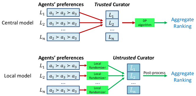
Figure 1: Comparison of two DP models

The main contribution of our work is LDP-KwikSort, an effective and efficient LDP protocol for the LDP-RA problem.

1. Instead of adding noise into the whole ranking list on each agent’s side, we focus on protecting the pairwise comparison preferences within the ranking list. To achieve that, we leverage on the approximate rank aggregation algorithm KwikSort [1, 2], which only requires the input as agents’ pairwise preferences. Based on this, the protocol allows the untrusted curator to ask the agents with pairwise comparison queries and lets the agents report their differentially private answers with the RR mechanism or the Laplace mechanism. By the post-processing algorithm, the untrusted data curator can approximately estimate the useful frequencies for rank aggregation and further output an aggregate ranking.

2. When adopting the RR mechanism and Laplace mechanism as the local randomizer for constructing the local perturbation algorithm, it comes up with the question of how should we choose an appropriate number of queries $K$ which is also the times of invoking the local randomizer. By analyzing the estimation error bound of aggregate pairwise comparison profile $\texttt{cmp}(\textbf{L})$ in the LDP-KwikSort protocol, we show that the utility can achieve the approximate maximum value around $K=\frac{\epsilon}{2}$, which is then further verified by extensive experiments.

3. For performance evaluation, we conduct experiments on three real-world datasets (TurkDots, TurkPuzzle and SUSHI) and several synthetic datasets generated from the Mallows model. By observing the error rate and the average Kendall tau distance resulted from the two solutions of LDP-KwikSort, the central model based solution DP-KwikSort [21] and the non-private KwikSort, it shows that our protocol especially the solution LDP-KwikSort:RR can achieve strong local privacy protection while maintaining an acceptable utility.

The rest of this paper is organized as follows. Section 2 provides the background on non-private and private rank aggregation, local differential privacy and its relaxed definition. Section 3 reviews the related work on differentially private voting mechanisms. Section 4 formalizes the LDP-RA problem and proposes the LDP-KwikSort protocol, followed by theoretical analysis in Section 5, empirical analysis in Section 6, and conclusions in Section 7.

2 Preliminaries

In this section, we introduce the relevant concepts of rank aggregation, private rank aggregation, the building blocks of LDP protocol, and a relaxation of differential privacy. Table 1 lists the notations used in this paper.

Table 1: Notations

$N$	set of agent $i$, where $N=\{1,...,n\}$
$A$	set of alternative $a_{j}$, where $A=\{a_{1},...,a_{m}\}$
$\mathcal{L}(A)$	all the possible permutations of elements in $A$
$L_{i}$	ranking preference profile of agent $i$, where $L_{i}\in\mathcal{L}(A)$
$L_{i}^{-1}(a_{j})$	ranking index of alternative $a_{j}$ in $L_{i}$
L	combined profile of all the agents’ preferences
$L_{(\textbf{L})}$	aggregate ranking over the given combined profile L
$\textbf{K}(L_{(\textbf{L})},L_{i})$	Kendall tau distance between $L_{(\textbf{L})}$ and $L_{i}$
$\overline{\textbf{K}}(L_{(\textbf{L})},\textbf{L})$	average Kendall tau distance between $L_{(\textbf{L})}$ and L
$C_{a_{j}a_{l}}(\textbf{L})$	count of the times that $L^{-1}(a_{j})<L^{-1}(a_{l})$ in L
$\texttt{cmp}_{\textbf{L}}(a_{j},a_{l})$	computing $C_{a_{j}a_{l}}(\textbf{L})-C_{a_{l}a_{j}}(\textbf{L})$
$\texttt{cmp}(\textbf{L})$	set of all the values of $\texttt{cmp}_{\textbf{L}}(a_{j},a_{l})$
$\widetilde{L}_{\mathcal{P}}$	aggregate ranking by the proposed protocol
$\epsilon$	overall privacy budget for each agent
$K$	number of queries from the curator to each agent
$\theta$	dispersion parameter of the Mallows model

2.1 Rank Aggregation

Given a set of $m$ alternatives $A=\{a_{1},...,a_{m}\}$ and $n$ agents participated in a preference aggregation procedure, the preference profile of an agent $i$ is represented as a permutation or a ranking $L_{i}\in\mathcal{L}(A)$ of those $m$ alternatives. Hence, the ranking index of alternative $a_{j}$ in $L_{i}$ is denoted by $L_{i}^{-1}(a_{j})$ with a value between $0$ (the best) to $m-1$ (the worst). Then a combined profile of these ranking preference profiles is denoted by $\textbf{L}=(L_{1},...,L_{n})\in\mathcal{L}(A)^{n}$, based on which, the rank aggregation algorithm generates a representative ranking $L_{(\textbf{L})}$ that sufficiently summarizes L.

To evaluate the quality of the aggregate ranking $L_{(\textbf{L})}$, Kendall tau distance is commonly used to count the number of pairwise disagreements between two rankings: $\textbf{K}(L_{(\textbf{L})},L_{i})=|\{(a_{j},a_{l}):a_{j}<a_{l},L_{(\textbf{L})}^{-1}(a_{j})<L_{(\textbf{L})}^{-1}(a_{l})\ but\ L^{-1}_{i}(a_{j})>L^{-1}_{i}(a_{l})\}|$. Then given the combined profile L, its average Kendall tau distance with an aggregate ranking $L_{(\textbf{L})}$ is defined as: $\overline{\textbf{K}}(L_{(\textbf{L})},\textbf{L})=\frac{1}{n}\sum_{i\in N}\textbf{K}(L_{(\textbf{L})},L_{i})$. When the above distance achieves the minimum, the relevant $L_{(\textbf{L})}$ is referred to as the Kemeny optimal aggregate ranking. However, it is NP-hard to compute this kind of ranking when $n>3$, and various approximate algorithms have been proposed as summarized in [8].

In this paper, we leverage on a Kendall tau distance based algorithm, KwikSort, which could achieve $11/7$-approximation by adopting the QuickSort strategy [2]. Specifically, the sorting of any two alternatives $a_{j},a_{l}\in A$ is based on the counts of how many times $a_{j}$ (resp. $a_{l}$) is preferred over $a_{l}$ (resp. $a_{j}$) among the rankings in L, which is formally defined as $C_{a_{j}a_{l}}(\textbf{L})=|\{for\ all\ L_{i}\in\textbf{L}|L_{i}^{-1}(a_{j})<L_{i}^{-1}(a_{l})\}|$ and $C_{a_{l}a_{j}}(\textbf{L})=|\{for\ all\ L_{i}\in\textbf{L}|L_{i}^{-1}(a_{l})<L_{i}^{-1}(a_{j})\}|$. Upon execution, KwikSort would first randomly pick an alternative $a_{p}\in A$ as the pivot, then classify all alternatives $a_{q}\in A\setminus\{a_{p}\}$ using the comparison function $\texttt{cmp}_{\textbf{L}}(a_{p},a_{q})=\left(C_{a_{p}a_{q}}(\textbf{L})-C_{a_{q}a_{p}}(\textbf{L})\right)\in\texttt{cmp}(\textbf{L})$. That is, if $\texttt{cmp}_{\textbf{L}}(a_{p},a_{q})<0$, the alternative $a_{q}$ would be classified into the left side of the pivot $a_{p}$, and vice versa. In particular, when $\texttt{cmp}_{\textbf{L}}(a_{p},a_{q})=0$, this placement can be done randomly. This procedure repeats until all alternatives have been sorted into a ranking ${L}_{KS}$. In the experiments of this paper, we adopt the Python package pwlistorder to help implement KwikSort algorithm, and the randomized placement method is adopted instead of its default method that directly places $a_{q}$ after $a_{p}$ if $\texttt{cmp}_{\textbf{L}}(a_{p},a_{q})=0$.

2.2 Private Rank Aggregation

Rank aggregation under the differential privacy framework is relatively new in the relevant community. [43, 21] considered the central model of DP in which the trusted data curator has access to all agents’ ranking preference profiles and would release the aggregate ranking by applying a differentially private algorithm $\mathcal{M}$ on them:

Definition 1 ($\epsilon$-differential privacy [16]).

A randomized algorithm $\mathcal{M}$ satisfies $\epsilon$-differential privacy if for all $\mathcal{O}\subseteq Range(\mathcal{M})$ and for all neighboring datasets L and $\textbf{L}^{\prime}$ differing on at most one record $L_{i}$ (i.e., the ranking preference profile of agent $i$), we have

$$Pr[\mathcal{M}(\textbf{L})\in\mathcal{O}]\leq e^{\epsilon}\cdot Pr[\mathcal{M}(\textbf{L}^{\prime})\in\mathcal{O}].$$

The intuition behind the above definition is that the adversary cannot confidently distinguish two outputs (aggregate rankings) of the differentially private algorithm $\mathcal{M}$ on a dataset L and its neighboring dataset $\textbf{L}^{\prime}$, where $\textbf{L},\textbf{L}^{\prime}\in\mathcal{D}$. Then the present or absent status of any agent’s ranking as a record within the input dataset is rigorously protected with the uncertainty of the algorithm’s outputs, which is measured by the privacy budget $\epsilon$.

To satisfy the definition of differential privacy and for those query functions $f$ with numeric output, the Laplace mechanism is usually utilized. Relying on the strategy of adding the Laplacian random variables (noise) to the query result, the Laplace mechanism can be formally defined as follows:

Definition 2 (Laplace mechanism [16]).

Given a function $f:\mathcal{D}\rightarrow\mathbb{R}^{k}$, the Laplace mechanism is defined as

$\mathcal{M}_{Lap}(\textbf{L})=f(\textbf{L})+(X_{1},...,X_{k})$,

where $X_{i}$ is i.i.d random variables drawn from $\textsf{Lap}(\frac{\Delta_{g}f}{\epsilon})$, and the global sensitivity of $f$ is $\Delta_{g}f=\max\limits_{\begin{subarray}{c}\textbf{L},\textbf{L}^{\prime}\in\mathcal{D}\\ \|{\textbf{L}-\textbf{L}^{\prime}}\|_{1}=1\end{subarray}}\|{f(\textbf{L})-f(\textbf{L}^{\prime})}\|_{1}$.

2.3 Local Differential Privacy

Unlike the central model, in the local model of DP [27, 14, 15], each agent would first locally perturb his/her data by adopting a randomized algorithm, referred to as the local randomizer $\mathcal{M}_{R}$, which satisfies $\epsilon$-differential privacy. Then, the agent would upload the perturbed data to the untrusted curator, who should not infer the sensitive information of each agent but can post-process those data to obtain the population statistics for further analysis. The local differential privacy is formally defined as follows:

Definition 3 ($\epsilon$-local differential privacy [17, 4]).

For a protocol $\mathcal{P}$ and dataset $D=(D_{1},...,D_{n})$, if $\mathcal{P}$ accesses $D$ only via $K$ invocations of a local randomizer $\mathcal{M}_{R}$ and each invocation satisfies $\epsilon_{k}$-differential privacy, which means that for any neighboring pair of datasets $D_{i}$, $D_{i}^{\prime}$ $\in D$ and $\forall\mathcal{O}\subseteq Range(\mathcal{M}_{R})$, if $\mathcal{M}_{R}$ satisfies

$$Pr[\mathcal{M}_{R}(D_{i})\in\mathcal{O}]\leq e^{\epsilon_{k}}\cdot Pr[\mathcal{M}_{R}(D_{i}^{\prime})\in\mathcal{O}]$$

and $\sum_{k=1}^{K}\epsilon_{k}\leq\epsilon$, then the protocol $\mathcal{P}(\cdot)\triangleq\left(\mathcal{M}_{R}^{(1)}(\cdot),\mathcal{M}_{R}^{(2)}(\cdot),\ldots,\mathcal{M}_{R}^{(K)}(\cdot)\right)$ satisfies $\epsilon$-local differential privacy ($\epsilon$-LDP).

To design LDP protocols, the randomized response (RR) mechanism [49, 19, 10] has been widely adopted. As an indirect questioning mechanism for sensitive questionnaires, RR allows the participating agents $i\in N$ to answer questions with plausible deniability. Specifically, assume that the true answers for $v_{i}$ is binary $v_{i}\in\{0,1\}$, each agent answers truthfully $u_{i}=v_{i}$ with probability $\frac{e^{\epsilon}}{e^{\epsilon}+1}$, and falsely $u_{i}=\overline{v_{i}}$ with probability $\frac{1}{e^{\epsilon}+1}$ [48, 22, 47]. These probabilities $p_{u_{i},v_{i}}$ then constitute a transformation matrix as

$$\textbf{M}=\begin{pmatrix}p_{0,0}&p_{0,1}\\ p_{1,0}&p_{1,1}\end{pmatrix}\ =\begin{pmatrix}\frac{e^{\epsilon}}{e^{\epsilon}+1}&\frac{1}{e^{\epsilon}+1}\\ \frac{1}{e^{\epsilon}+1}&\frac{e^{\epsilon}}{e^{\epsilon}+1}\end{pmatrix}.$$

Based on the knowledge of M, once obtaining $y_{0}$ (or $y_{1}$), the number of agents who answer ‘$0$’ (or ‘$1$’), the curator can use the unbiased maximum likelihood estimate (MLE) [23, 20, 42] to obtain an estimation $\widehat{x}_{0}$ (or $\widehat{x}_{1}$), which approximates the number of agents whose true answer are ‘$0$’ (or ‘$1$’).

$$\overrightarrow{\widehat{X}}=\textbf{M}^{-1}\overrightarrow{Y},$$ (1)

where $\overrightarrow{\widehat{X}}=(\widehat{x}_{0},\widehat{x}_{1})^{\tau}$, $\overrightarrow{Y}=(y_{0},y_{1})^{\tau}$, and $\textbf{M}^{-1}$ is the inverse matrix of M.

2.4 A Relaxation of Differential Privacy

Since the standard definition of differential privacy requires the strict distortion of analytical results which may lead to the significant reduction of utility in practical implementations, several relaxed definitions of differential privacy have been proposed such as the $(\epsilon,\delta)$-differential privacy, the individual differential privacy, and the Rényi differential privacy. Among them, the individual differential privacy (iDP) focuses on the indistinguishability between the actual dataset and its neighboring datasets instead of any pair of neighboring datasets, which is defined as follows:

Definition 4 ($\epsilon$-individual differential privacy [45]).

Given a dataset L, a randomized algorithm $\mathcal{M}$ satisfies $\epsilon$-individual differential privacy if for all $\mathcal{O}\subseteq Range(\mathcal{M})$ and for any dataset $\textbf{L}^{\prime}$ that is a neighbor of L, we have

$$Pr[\mathcal{M}(\textbf{L})\in\mathcal{O}]\leq e^{\epsilon}\cdot Pr[\mathcal{M}(\textbf{L}^{\prime})\in\mathcal{O}].$$

To satisfy the $\epsilon$-iDP, the Laplace mechanism can be also applied, but the sensitivity of a given function $f$ in Definition 2 should be replaced with the local sensitivity:

Definition 5 (Local sensitivity [38]).

Given a function $f:\mathcal{D}\rightarrow\mathbb{R}^{d}$, its local sensitivity at L is

$$\Delta_{l}f(\textbf{L})=\max\limits_{y:\|{\textbf{L}-y}\|_{1}=1}\|{f(\textbf{L})-f(y)}\|_{1}.$$

If we consider the individual differential privacy under the local model, it is natural to obtain the definition of the local individual differential privacy (LiDP) as follows:

Definition 6 ($\epsilon$-local individual differential privacy).

For a protocol $\mathcal{P}$ and dataset $D=(D_{1},...,D_{n})$, if $\mathcal{P}$ accesses $D$ only via $K$ invocations of a local randomizer $\mathcal{M}_{R}$ and each invocation satisfies $\epsilon_{k}$-individual differential privacy, which means that for any neighboring dataset $D_{i}^{\prime}$ of the given dataset $D_{i}$ and $\forall\mathcal{O}\subseteq Range(\mathcal{M}_{R})$, if $\mathcal{M}_{R}$ satisfies

$$Pr[\mathcal{M}_{R}(D_{i})\in\mathcal{O}]\leq e^{\epsilon_{k}}\cdot Pr[\mathcal{M}_{R}(D_{i}^{\prime})\in\mathcal{O}]$$

and $\sum_{k=1}^{K}\epsilon_{k}\leq\epsilon$, then the protocol $\mathcal{P}(\cdot)\triangleq\left(\mathcal{M}_{R}^{(1)}(\cdot),\mathcal{M}_{R}^{(2)}(\cdot),...,\mathcal{M}_{R}^{(K)}(\cdot)\right)$ satisfies $\epsilon$-local differential privacy ($\epsilon$-LiDP).

3 Related Work

In this section, we review some representative works on differentially private voting mechanisms. Under the central model of DP, Chen et al. [11, 12] considered to model privacy in players utility functions for achieving both of privacy preservation and truthfulness, and proposed mechanism for private two-candidate election; Lee [29] proposed an algorithm that satisfies both $\epsilon$-DP and $\epsilon$-strategyproof for tournament voting rules. Considering the rank aggregation scenario, Shang et al. [43] introduced a relaxed DP definition, $(\epsilon,\delta)$-DP, into the differentially private algorithm to release the histogram of rankings with the utility bounds analyzed. Then in the work of Hay et al. [21], three differentially private algorithms were proposed by separately concentrating on the approximate and the optimal rank aggregation. Among them, DP-KwikSort algorithm extends the approximate rank aggregation algorithm KwikSort by the Laplace mechanism.

Under the local model of DP, the private algorithms for majority voting and truth discovery [32, 33], weighted voting [52], and positional voting [46] were designed. Besides, Liu et al. [34] explored the theoretical relationship between the internal randomness of certain voting rules and the privacy-preserving level. However, to the best of our knowledge, no existing work has been devoted to rank aggregation under the local model of DP which is introduced in the next section.

4 Locally Private Rank Aggregation

In this section, we formalize the problem of locally differentially private rank aggregation (LDP-RA) and then propose a solution called LDP-KwikSort protocol.

4.1 Problem Formalization

There are $n$ agents that own their ranking profile $L_{i}$ over $m$ alternatives. In the context of LDP-RA, the combined profile $\textbf{L}=(L_{1},...,L_{n})$ can be considered as an instantiation of $D=(D_{1},...,D_{n})$ in Definition 3. The task is then to design a local randomizer $\mathcal{M}_{R}$ which locally perturbs each agent’s ranking preference profile $L_{i}$ before reporting to the untrusted curator. On the other hand, we expect that the constituted $\epsilon$-LDP protocol (or $\epsilon$-LiDP protocol) $\mathcal{P}$ outputs the aggregate ranking $\widetilde{L}_{\mathcal{P}}$ with an acceptable utility as measured by the average Kendall tau distance $\overline{\textbf{K}}(\widetilde{L}_{\mathcal{P}},\textbf{L})=\frac{1}{n}\sum_{i\in N}\textbf{K}(\widetilde{L}_{\mathcal{P}},L_{i})$.

4.2 Protocol Overview

To solve the LDP-RA problem, we propose the locally differentially private KwikSort (LDP-KwikSort) protocol which contains two solutions: LDP-KwikSort:RR and LDP-KwikSort:Lap, and the rationale of the former can be summarized in Figure 2.

When executing the LDP-KwikSort protocol, $K$ rounds of interactions exist between every agent and the curator. In each interaction, the curator randomly selects $K$ different pairs of alternatives for querying, and the agent reports the answer. These queries are predefined as do you prefer the alternative $a_{j}$ to $a_{l}$?. When receiving the query, the agent adopts RR mechanism to report the perturbed answer (Algorithm 1). After collecting the answers from all agents, the curator aggregates these data and estimates the needed statistics which can be further used by the KwikSort algorithm. Finally, the KwikSort algorithm is executed to generate an aggregate ranking (Algorithm 2).

Figure 2: Rationale for LDP-KwikSort:RR Solution

4.3 Local Perturbation

As shown in Algorithm 1, when receiving the $K$ queries, an agent $i\in N$ adopts the standard RR mechanism as the local randomizer $\mathcal{M}_{R}$, and reports the curator with the perturbed answer $\widetilde{\textbf{o}}_{i}$. Here, we adopt the transformation matrix $\textbf{M}_{rr}$ introduced in Section 2.3 to include the coin flipping probabilities $p_{\widetilde{o}_{ik},o_{ik}}$ of a true answer $o_{ik}$ being transformed into the reported answer $\widetilde{o}_{ik}$. Let $\textbf{M}_{rr}$ be the common knowledge of the agents and the curator:

$$\textbf{M}_{rr}=\begin{pmatrix}p_{0,0}&p_{0,1}\\ p_{1,0}&p_{1,1}\\ \end{pmatrix}=\begin{pmatrix}p_{rr}&1-p_{rr}\\ 1-p_{rr}&p_{rr}\\ \end{pmatrix}$$

where all the diagonal elements get assigned the value $p_{rr}$ while $1-p_{rr}$ for other elements, and $p_{rr}=\frac{e^{\epsilon_{k}}}{e^{\epsilon_{k}}+1}$, $\epsilon_{k}=\epsilon/K$.

Algorithm 1 Local Perturbation in LDP-KwikSort:RR

1:Agent $i$’s ranking profile $L_{i}$, $K$ queries, transformation matrix $\textbf{M}_{rr}$

2:Agent $i$’s perturbed answer $\widetilde{\textbf{o}}_{i}$

3:Receives $K$ queries (e.g., do you prefer alternative $a_{j}$ to $a_{l}$?) from curator

4:for each query $k\in[K]$ do

5:    Randomly generates a number $g$ from $[0,1]$ $\triangleright$ Local Randomizer $\mathcal{M}_{R}$

6:    if $g\leq p_{rr}$ then

7:         $\widetilde{o}_{ik}\leftarrow 1$

8:    else

9:         $\widetilde{o}_{ik}\leftarrow 0$

10:    end if

11:end for

12:Agent $i$ reports the perturbed answer $\widetilde{\textbf{o}}_{i}=\{\widetilde{o}_{i1},...,\widetilde{o}_{iK}\}$ to curator

4.4 Post-processing

As shown in Algorithm 2, once collected the answers from the agents, firstly (Line $1-9$), the curator classifies these noisy data. For each possible pair of alternatives $a_{j}$ and $a_{l}$, two counters $\widetilde{C}_{a_{j}a_{l}}(\textbf{L})$ and $\widetilde{C}_{a_{l}a_{j}}(\textbf{L})$ are updated to indicate the numbers of the agent who prefers alternative $a_{j}$ (or $a_{l}$) to alternative $a_{l}$ (or $a_{j}$). Secondly (Line $10-13$), the curator obtains the estimations of $C_{a_{j}a_{l}}(\textbf{L})$ and $C_{a_{l}a_{j}}(\textbf{L})$ by Equation 1, where $\overrightarrow{\widehat{X}}=\left(\widehat{C}_{a_{j}a_{l}}(\textbf{L}),\widehat{C}_{a_{l}a_{j}}(\textbf{L})\right)$, $\overrightarrow{Y}=\left(\widetilde{C}_{a_{j}a_{l}}(\textbf{L}),\widetilde{C}_{a_{l}a_{j}}(\textbf{L})\right)^{\tau}$. Then the results from the comparison function $\widehat{\texttt{cmp}}_{\textbf{L}}(a_{j},a_{l})$ can be computed. Finally (Line $14-15$), the curator assembles all the values of $\widehat{\texttt{cmp}}_{\textbf{L}}(a_{j},a_{l})$ into the estimated version of aggregate pairwise comparison profile $\widehat{\texttt{cmp}}(\textbf{L})$. By taking $\widehat{\texttt{cmp}}(\textbf{L})$ as input, the standard KwikSort algorithm is executed to generate an aggregate ranking $\widetilde{L}_{\mathcal{P}}$.

Algorithm 2 Post-processing in LDP-KwikSort:RR

1:Agents’ perturbed answers $\widetilde{\textbf{o}}=\{\widetilde{\textbf{o}}_{1},...,\widetilde{\textbf{o}}_{n}\}$, transformation matrix $\textbf{M}_{rr}$

2:Aggregate ranking $\widetilde{L}_{\mathcal{P}}$

3:for $\widetilde{\textbf{o}}_{i}\in\widetilde{\textbf{o}}$ do $\triangleright$ Classification

4:    for $\widetilde{o}_{ik}\in\widetilde{\textbf{o}}_{i}$ do

5:         if $\widetilde{o}_{ik}=1$ then

6:             $\widetilde{C}_{a_{j}a_{l}}(\textbf{L})+1$

7:         else

8:             $\widetilde{C}_{a_{l}a_{j}}(\textbf{L})+1$

9:         end if

10:    end for

11:end for

12:for each possible pair $(a_{j},a_{l})$ do $\triangleright$ Estimation and computation

13:    Obtains two estimations $\widehat{C}_{a_{j}a_{l}}(\textbf{L})$ and $\widehat{C}_{a_{l}a_{j}}(\textbf{L})$ by  Equation 1

14:    $\widehat{\texttt{cmp}}_{\textbf{L}}(a_{j},a_{l})\leftarrow\widehat{C}_{a_{j}a_{l}}(\textbf{L})-\widehat{C}_{a_{l}a_{j}}(\textbf{L})$

15:end for

16:Obtains $\widehat{\texttt{cmp}}(\textbf{L})$ and executes KwikSort algorithm

17:return Aggregate ranking $\widetilde{L}_{\mathcal{P}}$

4.5 Laplace Solution

Since the agent $i$’s perturbed answer $\widetilde{\textbf{o}}_{i}$ contains numeric values, we also propose the Laplace mechanism based solution LDP-KwikSort:Lap.

Local perturbation.

As shown in Algorithm 3, when receiving the $K$ queries, an agent $i\in N$ adopts the Laplace mechanism as the local randomizer $\mathcal{M}_{R}$, and reports the curator with the perturbed answer $\widetilde{\textbf{o}}_{i}$. Here, $f_{o}(\cdot)$ is a query function which takes agent’s ranking preference as input and outputs $1$ or $0$ to indicate whether this agent prefers $a_{j}$ to $a_{l}$ or not, for default index $j<l$. Then the local sensitivity $\Delta_{l}f_{o}$ is $1$, which reflects the maximum change of its outputs.

Algorithm 3 Local Perturbation in LDP-KwikSort:Lap

1:Agent $i$’s ranking profile $L_{i}$, $K$ queries, privacy budget $\epsilon$

2:Agent $i$’s perturbed answer $\widetilde{\textbf{o}}_{i}$

3:Receives $K$ queries (e.g., do you prefer alternative $a_{j}$ to $a_{l}$?) from curator

4:for each query $k\in[K]$ do

5:    $\widetilde{o}_{ik}\leftarrow o_{ik}+X_{ldp}$ where $X_{ldp}\sim\textsf{Lap}(\frac{\Delta_{l}f_{o}}{\epsilon_{k}})$ $\triangleright$ Local Randomizer $\mathcal{M}_{R}$

6:end for

7:Agent $i$ reports the perturbed answer $\widetilde{\textbf{o}}_{i}=\{\widetilde{o}_{i1},...,\widetilde{o}_{iK}\}$ to curator

Post-processing.

As shown in Algorithm 4, once collected the answers from the agents, firstly (Line $1-9$), the curator also classifies these noisy data. For each possible pair of alternatives $a_{j}$ and $a_{l}$, two counters $\widehat{C}_{a_{j}a_{l}}(\textbf{L})$ and $\widehat{C}_{a_{l}a_{j}}(\textbf{L})$ are updated. Note that these counters are the estimations of $C_{a_{j}a_{l}}(\textbf{L})$ and $C_{a_{l}a_{j}}(\textbf{L})$, and the updates are based on judging whether $\widetilde{o}_{ik}\geq 0.5$, which is different from the approach in Algorithm 2. Secondly (Line $10-12$), the curator obtains $\widehat{\texttt{cmp}}_{\textbf{L}}(a_{j},a_{l})$ by directly subtracting $\widehat{C}_{a_{l}a_{j}}(\textbf{L})$ from $\widehat{C}_{a_{j}a_{l}}(\textbf{L})$. Finally (Line $13-14$), the curator assembles all the values of $\widehat{\texttt{cmp}}_{\textbf{L}}(a_{j},a_{l})$ into the estimated version of aggregate pairwise comparison profile $\widehat{\texttt{cmp}}(\textbf{L})$. By taking $\widehat{\texttt{cmp}}(\textbf{L})$ as input, the standard KwikSort algorithm is executed to generate an aggregate ranking $\widetilde{L}_{\mathcal{P}}$.

Algorithm 4 Post-processing in LDP-KwikSort:Lap

1:Agents’ perturbed answers $\widetilde{\textbf{o}}=\{\widetilde{\textbf{o}}_{1},...,\widetilde{\textbf{o}}_{n}\}$

2:Aggregate ranking $\widetilde{L}_{\mathcal{P}}$

3:for $\widetilde{\textbf{o}}_{i}\in\widetilde{\textbf{o}}$ do $\triangleright$ Classification

4:    for $\widetilde{o}_{ik}\in\widetilde{\textbf{o}}_{i}$ do

5:         if $\widetilde{o}_{ik}\geq 0.5$ then

6:             $\widehat{C}_{a_{j}a_{l}}(\textbf{L})+1$

7:         else

8:             $\widehat{C}_{a_{l}a_{j}}(\textbf{L})+1$

9:         end if

10:    end for

11:end for

12:for each possible pair $(a_{j},a_{l})$ do $\triangleright$ Computation

13:    $\widehat{\texttt{cmp}}_{\textbf{L}}(a_{j},a_{l})\leftarrow\widehat{C}_{a_{j}a_{l}}(\textbf{L})-\widehat{C}_{a_{l}a_{j}}(\textbf{L})$.

14:end for

15:Obtains $\widehat{\texttt{cmp}}(\textbf{L})$ and executes KwikSort algorithm

16:return Aggregate ranking $\widetilde{L}_{\mathcal{P}}$

5 Theoretical Analysis

In this section, we provide the privacy and utility guarantees, as well as the computational complexity of the proposed LDP-KwikSort protocol.

5.1 Privacy Guarantee

We have the following theorem on the privacy guarantee of the LDP-KwikSort protocol.

Theorem 1.

LDP-KwikSort:RR satisfies $\epsilon$-LDP and LDP-KwikSort:Lap satisfies $\epsilon$-LiDP.

Proof. We respectively analyze two solutions of LDP-KwikSort protocol as follows:

1. In the local perturbation algorithm, since the solution LDP-KwikSort:RR adopts the transformation matrix based local randomizer $\mathcal{M}_{R}$ to perturb each answer from the agent, we have

   $$\frac{Pr[\mathcal{M}_{R}(o_{ik}=u)=u]}{Pr[\mathcal{M}_{R}(o_{ik}=v)=u]}=\frac{2p_{rr}}{1-p_{rr}}=e^{\epsilon_{k}}.$$

   Based on Definition 1, we can conclude that the local randomizer $\mathcal{M}_{R}$ in solution LDP-KwikSort:RR satisfies $\epsilon_{k}$-DP.

2. In the local perturbation algorithm, since the solution LDP-KwikSort:Lap adopts the local sensitivity based Laplace mechanism to design the local randomizer $\mathcal{M}_{R}$ for perturbing each answer from the agent, based on Definition 4, we can conclude that the local randomizer $\mathcal{M}_{R}$ in solution LDP-KwikSort:Lap satisfies $\epsilon_{k}$-iDP.

Consequently, according to Definition 3, we can conclude that LDP-KwikSort:RR satisfies $\epsilon$-LDP and LDP-KwikSort:Lap satisfies $\epsilon$-LiDP, where $\epsilon=K\cdot\epsilon_{k}$.       

5.2 Utility Guarantee

5.2.1 Analysis of LDP-KwikSort:RR

As described in Algorithm 2, the post-processing procedure on the side of the curator mainly contains two parts: the estimation of $\texttt{cmp}(\textbf{L})$ from the noisy data, and the execution of the KwikSort algorithm. It is known that KwikSort can output an $11/7$-optimal aggregate ranking with a given aggregate pairwise comparison profile $\texttt{cmp}(\textbf{L})$. Therefore, it is important to measure the error of estimating $\texttt{cmp}(\textbf{L})$ from the first part, which indicates the gap between the aggregate ranking $\widetilde{L}_{\mathcal{P}}$ from KwikSort protocol and the $11/7$-optimal aggregate ranking ${L}_{KS}$. When investigating the internal disagreements of the original aggregate pairwise comparison profile $\texttt{cmp}(\textbf{L})$ and its estimated version $\widehat{\texttt{cmp}}(\textbf{L})$, we use Equation 1 to obtain

$$\textbf{M}_{rr}\overrightarrow{\widehat{X}}=\overrightarrow{Y},$$

That is

$$\begin{pmatrix}p_{rr}&1-p_{rr}\\ 1-p_{rr}&p_{rr}\end{pmatrix}\begin{pmatrix}\widehat{C}_{a_{j}a_{l}}(\textbf{L})\\ \widehat{C}_{a_{l}a_{j}}(\textbf{L})\end{pmatrix}=\begin{pmatrix}\widetilde{C}_{a_{j}a_{l}}(\textbf{L})\\ \widetilde{C}_{a_{l}a_{j}}(\textbf{L})\end{pmatrix}.$$

Expend the equation, we have

$$\widehat{\texttt{cmp}}_{\textbf{L}}(a_{j},a_{l})=\widehat{C}_{a_{j}a_{l}}(\textbf{L})-\widehat{C}_{a_{l}a_{j}}(\textbf{L})=\frac{\widetilde{C}_{a_{j}a_{l}}(\textbf{L})-\widetilde{C}_{a_{l}a_{j}}(\textbf{L})}{p_{rr}-(1-p_{rr})}=\frac{\widetilde{\texttt{cmp}}_{\textbf{L}}(a_{j},a_{l})}{2p_{rr}-1}.$$ (2)

Since the denominator $(2p_{rr}-1)>0$ when $\epsilon_{k}>0$, we can conclude that the sign of $\widehat{\texttt{cmp}}_{\textbf{L}}(a_{j},a_{l})$ is the same as that of $\widetilde{\texttt{cmp}}_{\textbf{L}}(a_{j},a_{l})$. As the KwikSort algorithm determines the relative order of alternatives $(a_{j},a_{l})$ only by checking the sign of $\texttt{cmp}_{\textbf{L}}(a_{j},a_{l})$, we turn to measure the probability that the sign of $\widetilde{\texttt{cmp}}_{\textbf{L}}(a_{j},a_{l})$ is different with that of $\texttt{cmp}_{\textbf{L}}(a_{j},a_{l})$. That is to say, the achieved utility of LDP-KwikSort relies on the condition that for the ground truth $L_{(\textbf{L})}^{-1}(a_{j})<L_{(\textbf{L})}^{-1}(a_{l})$ whether the curator can directly obtain it by just observing the noisy data from the agents. Besides, when $\widetilde{\texttt{cmp}}_{\textbf{L}}(a_{j},a_{l})$ and $\texttt{cmp}_{\textbf{L}}(a_{j},a_{l})$ have the same sign, the difference between their absolute values will not impact on the utility of solution LDP-KwikSort:RR.

Next, we present an error bound and the associated proof, which are based on the assumption that the agents’ ranking preference profiles are generated by the Mallows model. The Mallows model [35] is a probabilistic model for ranking generation in which the probability of generating a ranking is based on the dispersion parameter $\theta\in[0,1]$ and the distance between this ranking and a ground truth ranking. Specifically, $\theta=1-\frac{q_{M}}{p_{M}}$ where $p_{M}\in[\frac{1}{2},1]$ is the probability for generating the relative order of alternatives $(a_{j},a_{l})$ which is consistent with the ground truth and $q_{M}=1-p_{M}$ is the opposite probability.

Theorem 2.

If all the ranking preference profiles are generated by the Mallows model with the dispersion parameter $\theta$ and a ground truth ranking, the estimation of $\texttt{cmp}(\textbf{L})$ by LDP-KwikSort:RR produces the error $<6\mu$ with probability at least $1-2^{-6\mu}$, where $\mu=2\binom{m}{2}\exp\left(-\frac{\epsilon^{2}K}{(\epsilon+2K)^{2}}\cdot\frac{{\theta^{*}}^{2}n}{m(m-1)}\right)$ and $\theta^{*}=\frac{\theta}{2-\theta}$.

Proof. In our scenario, for a certain pairwise comparison query such that ‘for alternative pair $(a_{j},a_{l})$, whether $L_{i}^{-1}(a_{j})<L_{i}^{-1}(a_{l})$ or not’, there will be $n^{*}=n\frac{K}{\binom{m}{2}}$ agents involved, and each agent reports his/her true answer (resp. false answer) with probability $p_{rr}=\frac{e^{\epsilon_{k}}}{e^{\epsilon_{k}}+1}$ (resp. $q_{rr}=1-p_{rr}=\frac{1}{e^{\epsilon_{k}}+1}$). When considering the assumption regarding the Mallows model, an agent finally reports the ground truth answer (i.e., $L_{i}^{-1}(a_{j})<L_{i}^{-1}(a_{l})$ for all $j<l$) with probability $\verb"p"=p_{M}\cdot p_{rr}+q_{M}\cdot q_{rr}$ and reports the opposite answer with probability $\verb"q"=p_{M}\cdot q_{rr}+q_{M}\cdot p_{rr}$.

Since the above procedure could be seen as a Bernoulli trial, here we adopt the variation of Hoeffding’s inequality [50] for Bernoulli trial as follows:

Lemma 1.

For a Bernoulli trial in which $n$ times of experiment have been conducted and each experiment outputs outcome $A$ with probability $\verb"p"$ and outcome $B$ with probability $\verb"q"=1-\verb"p"$, we have the following probability inequality for some $\delta>0$:

$$Pr[(\verb"p"-\delta)n\leq H(n)\leq(\verb"p"+\delta)n]\geq 1-2\exp(-2{\delta}^{2}n),$$

where $H(n)$ is the number of outcome $A$ in $n$ experiments.

We then have the following probability inequalities by Lemma 1:

$$Pr[(\verb"p"-\delta)n^{*}\leq\widetilde{C}_{a_{j}a_{l}}(\textbf{L})\leq(\verb"p"+\delta)n^{*}]\geq 1-2\exp(-2{\delta}^{2}n^{*}),$$

$$Pr[(\verb"q"-\delta)n^{*}\leq\widetilde{C}_{a_{l}a_{j}}(\textbf{L})\leq(\verb"q"+\delta)n^{*}]\geq 1-2\exp(-2{\delta}^{2}n^{*}),$$

and hence

$$Pr[(\verb"p"-\verb"q"-2\delta)n^{*}\leq\widetilde{C}_{a_{j}a_{l}}(\textbf{L})-\widetilde{C}_{a_{l}a_{j}}(\textbf{L})\leq(\verb"p"-\verb"q"+2\delta)n^{*}]\geq 1-2\exp(-2{\delta}^{2}n^{*}).$$

If we let $\verb"p"-\verb"q"=2\delta$ and $\theta^{*}=\frac{\theta}{2-\theta}$, the following probability inequalities are obtained:

$$Pr[0\leq\widetilde{C}_{a_{j}a_{l}}(\textbf{L})-\widetilde{C}_{a_{l}a_{j}}(\textbf{L})\leq 4\delta n^{*}]\geq 1-2\exp(-2{\delta}^{2}n^{*})$$

and

$$Pr[\widetilde{\texttt{cmp}}_{\textbf{L}}(a_{j},a_{l})=\widetilde{C}_{a_{j}a_{l}}(\textbf{L})-\widetilde{C}_{a_{l}a_{j}}(\textbf{L})<0]<2\exp(-2{\delta}^{2}n^{*})=2\exp\left(-2(\frac{p_{M}\cdot p_{rr}+q_{M}\cdot q_{rr}-p_{M}\cdot q_{rr}-q_{M}\cdot p_{rr}}{2})^{2}n^{*}\right)=2\exp\left(-\frac{({p_{rr}-q_{rr}})^{2}{\theta^{*}}^{2}n^{*}}{2}\right)\approx 2\exp\left(-\frac{\epsilon^{2}K}{(\epsilon+2K)^{2}}\cdot\frac{{\theta^{*}}^{2}n}{m(m-1)}\right)=P_{\iota}.$$ (3)

This formula reflects the error bound of generating data and reporting answers by $n$ agents for a certain pair of alternatives $(a_{j},a_{l})$. Here, we adopt the inequality $e^{x}\geq x+1$ for simplifying the result in the last derivation.

After obtaining the error bound for a certain pairwise comparison query, we now apply the following Chernoff bound for all the possible queries:

Lemma 2.

Let $X_{1},...,X_{n}$ be independent Poisson trials such that $Pr(X_{i}=1)=p_{i}$. Let $X=\sum_{i=1}^{n}X_{i}$ and $\mu=\mathbf{E}[X]$. Then for $R\geq 6\mu$,

$$Pr(X\geq R)\leq 2^{-R}.$$

Therefore, we finish the proof with obtaining

$$\mu=\mathbf{E}[X]=\mathbf{E}[\sum_{\iota=1}^{\binom{m}{2}}X_{\iota}]=\sum_{\iota=1}^{\binom{m}{2}}\mathbf{E}[X_{\iota}]=\sum_{\iota=1}^{\binom{m}{2}}P_{\iota}\leq 2\binom{m}{2}\exp\left(-\frac{\epsilon^{2}K}{(\epsilon+2K)^{2}}\cdot\frac{{\theta^{*}}^{2}n}{m(m-1)}\right).$$

      

Based on Theorem 2, we can find that the estimation error of LDP-KwikSort:RR depends on the expectation $\mu$, and a smaller $\mu$ indicates a smaller error. Then we observe that 1) when the privacy budget $\epsilon$, the number of agents $n$ and alternatives $m$, and the dispersion parameter $\theta$ are fixed, $\mu$ is influenced by the function $g(K)=\frac{\epsilon^{2}K}{(\epsilon+2K)^{2}}$, and it gets the approximate minimum value when the number of queries $K=\frac{\epsilon}{2}$; 2) when more agents are involved or given a large privacy budget for each agent, i.e., $n\rightarrow\infty$ or $\epsilon\rightarrow\infty$, $\mu$ will be reduced to zero; 3) with increasing the number of alternatives $m$, $\mu$ is also increased; 4) when the dispersion parameter $\theta$ is relatively large, i.e., the generated rankings are closer to the ground truth ranking, we obtain a relatively small $\mu$. In Section 6, we conduct a series of experiments to verify these theoretical observations.

5.2.2 Analysis of LDP-KwikSort:Lap

As described in Algorithm 4, the post-processing procedure on the side of the curator also contains two parts: the estimation of $\texttt{cmp}(\textbf{L})$ from the noisy data, and the execution of the KwikSort algorithm. Its most difference with Algorithm 2 lies in using the threshold checking about $\widetilde{o}_{ik}$ instead of using Equation 1 to obtain $\widehat{C}_{a_{j}a_{l}}(\textbf{L})$ and $\widehat{C}_{a_{l}a_{j}}(\textbf{L})$. Then we have the expressions regarding $\widetilde{o}_{ik}$:

$$\widetilde{o}_{ik}=\begin{cases}0,&\text{if $o_{ik}+\textsf{Lap}(\frac{\Delta_{l}f_{o}}{\epsilon_{k}})<0.5$},\\ 1,&\text{if $o_{ik}+\textsf{Lap}(\frac{\Delta_{l}f_{o}}{\epsilon_{k}})\geq 0.5$}.\end{cases}$$

According to the cumulative distribution function of Laplacian random variables, we have the probabilities of a true answer $o_{i}$ being transformed into the reported answer $\widetilde{o}_{i}$ as

$$p_{\widetilde{o}_{ik},o_{ik}}=\begin{cases}p_{0,0}=F(0.5)=1-\frac{1}{2}\exp(-\frac{\epsilon_{k}}{2}),\\ p_{0,1}=1-F(0.5)=\frac{1}{2}\exp(-\frac{\epsilon_{k}}{2}),\\ p_{1,0}=F(-0.5)=\frac{1}{2}\exp(-\frac{\epsilon_{k}}{2}),\\ p_{1,1}=1-F(-0.5)=1-\frac{1}{2}\exp(-\frac{\epsilon_{k}}{2}),\end{cases}$$

and we further have the following transformation matrix:

$$\textbf{M}_{lap}=\begin{pmatrix}p_{0,0}&p_{0,1}\\ p_{1,0}&p_{1,1}\\ \end{pmatrix}=\begin{pmatrix}p_{lap}&1-p_{lap}\\ 1-p_{lap}&p_{lap}\\ \end{pmatrix},$$

where all the diagonal elements are assigned with the value $p_{lap}$ while $1-p_{lap}$ for other elements, and $p_{lap}=1-\frac{1}{2}\exp(-\frac{\epsilon_{k}}{2})$, $\epsilon_{k}=\epsilon/K$. Then we follow the analysis technique of LDP-KwikSort:RR and replace $p_{rr}$ with $p_{lap}$ in Equation 3 to obtain the following conclusion:

Theorem 3.

If all the ranking preference profiles are generated by the Mallows model with the dispersion parameter $\theta$ and a ground truth ranking, the estimation of $\texttt{cmp}(\textbf{L})$ by LDP-KwikSort:Lap produces the error $<6\mu$ with probability at least $1-2^{-6\mu}$, where $\mu=2\binom{m}{2}\exp\left(-(1-e^{-\frac{\epsilon}{2K}})^{2}K\cdot\frac{{\theta^{*}}^{2}n}{m(m-1)}\right)$ and $\theta^{*}=\frac{\theta}{2-\theta}$.

Based on Theorem 3, it is found that the estimation error of LDP-KwikSort:Lap also depends on the expectation $\mu$, and a smaller $\mu$ indicates a smaller error. We observe that when the privacy budget $\epsilon$, the number of agents $n$ and alternatives $m$, and the dispersion parameter $\theta$ are fixed, $\mu$ is influenced by the function $g(K)=(1-e^{-\frac{\epsilon}{2K}})^{2}K$, and it gets the approximate minimum value when the number of queries $K<\frac{\epsilon}{2}$. Other observations are the same as LDP-KwikSort:RR, and in the experiments we will verify these theoretical observations.

5.3 Computational Complexity

As shown in Table 2, we analyze the computational complexity of the proposed protocol with $K$ queries in terms of the following aspects:

Table 2: Computational complexity of LDP-KwikSort protocol

		Local perturbation	Post-processing
Time	Agent	$O(K)$
	Curator	$O(nK)$	$O(nK)+O(m^{2})+O(m\log m)$
Space	Agent	$O(\log K)$
	Curator	$O(n\log K)$	$O(n\log K)$
Communication	Agent	$O(\log K)$	$O(\log K)$
	Curator	$O(n\log K)$	$O(n\log K)$

Running time.

For each agent, in the local perturbation algorithm of solution LDP-KwikSort:RR, the basic operations are generating random number $K$ times and number comparison $K$ times, thus the complexity is $O(K)$. For that of LDP-KwikSort:Lap, since the basic operations are generating random number $K$ times and addition $K$ times, the complexity is also $O(K)$.

On the curator’s side, in the local perturbation algorithms of two solutions, it is required to generate $K$ queries to each agent, thus the complexity is $O(nK)$. For the post-processing algorithm, the complexities of the classification phase and the estimation & computation phase are $O(nK)$ and $O(\binom{m}{2})\approx O(m^{2})$, respectively. The execution of KwikSort algorithm consumes $O(m\log m)$. Thus, the total time complexity of the curator’s operation is $O(2nK)+O(m^{2})+O(m\log m)$.

Processing memory.

For each agent, the main processing memory lies in the $K$ queries, which consumes $O(\log K)$ bits. For the curator, as it maintains $n$ times the sums of at most $2K$ bits for each agent, the processing memory is $O(2n\log K)$ bits.

Communication cost.

The number of queries directly impacts the communication cost, which includes $O(2\log K)$ for each agent and $O(2n\log K)$ for the curator.

6 Empirical Analysis

In this section, we present the performance evaluation of the LDP-KwikSort protocol and the competitors on both real and synthetic datasets. Section 6.1 introduces the experiment settings, and Section 6.2-6.5 investigate how will the parameters (number of queries $K$, privacy budget $\epsilon$, number of agent $n$ and alternative $m$, and dispersion parameter $\theta$) impact on performance. Section 6.6 compares the time costs of involved solutions, and Section 6.7 provides a summarized discussion.

6.1 Experiment Settings

6.1.1 Competitors

KwikSort.

We adopt the approximate rank aggregation algorithm KwikSort described in [2] as the non-private solution. Since each agent responds to each query with the true answer to the curator, and the latter releases the aggregate ranking without adding any noise, the performances of KwikSort can be seen as the empirical error lower bound in our experiments.

DP-KwikSort.

We adopt the differentially private algorithm DP-KwikSort [21] as the solution under the central model of DP. When executing this algorithm, each agent responds to each query with the true answer to the curator, and the latter adopts the Laplace mechanism to introduce noises during the rank aggregation. Specifically, the algorithm adds noises into the results of the comparison function: $\widetilde{\texttt{cmp}}_{\textbf{L}}(a_{j},a_{l})=\texttt{cmp}_{\textbf{L}}(a_{j},a_{l})+X_{dp}$ where $X_{dp}\sim\textsf{Lap}(1/\epsilon^{\prime})$ and $\epsilon^{\prime}=\epsilon/((m-1)\log m)$. Besides, the number of queries in DP-KwikSort is defaulted as $K=\binom{m}{2}$.

6.1.2 Datasets and Configuration

The experiments are conducted on synthetic datasets and three real-world datasets (TurkDots, TurkPuzzle and SUSHI). Among them, datasets TurkDots and TurkPuzzle [36] were collected from the crowdsourcing marketplace Amazon Mechanical Turk, which respectively contains $n=795$ and $n=793$ agents’ full ranking preference profiles over $m=4$ alternatives. Dataset SUSHI [25] contains the full rankings of $m=10$ types of sushi from $n=5000$ agents in a questionnaire survey. The synthetic datasets were generated by the Mallows model with R package PerMallows $1.13$ [24].

The involved protocols and algorithms are implemented in Python $2.7$ based on the package pwlistorder $0.1$ [13], and executed on an Intel Core i$5-3210$M $2.50$GHz machine with $6$GB memory. In each experiment, the protocols and algorithms were tested $30$ times, and their mean score of the adopted utility metrics was reported.

6.1.3 Utility Metrics

Error rate.

In experiments we coin the measurement error rate to reflect how accurate the estimated version of aggregate pairwise comparison profile $\widehat{\texttt{cmp}}(\textbf{L})$ agrees with the ground truth $\texttt{cmp}(\textbf{L})$. Specifically, for all possible alternative pairs $a_{j}$ and $a_{l}$ where $j<l$,

$$ErrorRate=\frac{|\{\texttt{cmp}_{\textbf{L}}(a_{j},a_{l})>0\ and\ \widehat{\texttt{cmp}}_{\textbf{L}}(a_{j},a_{l})<0\}|}{\binom{m}{2}}$$ (4)

$$+\frac{|\{\texttt{cmp}_{\textbf{L}}(a_{j},a_{l})<0\ and\ \widehat{\texttt{cmp}}_{\textbf{L}}(a_{j},a_{l})>0\}|}{\binom{m}{2}}.$$

Average Kendall tau distance.

As mentioned before, we measure the achieved accuracy of the aggregate ranking $\widetilde{L}_{\mathcal{P}}$ by adopting the average Kendall tau distance $\overline{\textbf{K}}(\widetilde{L}_{\mathcal{P}},\textbf{L})=\frac{1}{n}\sum_{i\in N}\textbf{K}(\widetilde{L}_{\mathcal{P}},L_{i})$. Furthermore, for the convenience of comparison with different $m$, we normalize the values by $m(m-1)/2$.

6.2 The Impact of Query Amount

The number of queries determines the amount of provided information about each agent’s private ranking preference profile. Intuitively, a relatively large $K$ helps the curator to generate an approximate optimal aggregate ranking. However, for LDP-KwikSort protocol, since the overall privacy budget $\epsilon$ of each agent will be split into $K$ parts for reporting each query, a large number of queries will lead to more noises per answer, which may make the collected information chaotic. According to the theoretical analysis in Section 5.2, we observe that two solutions of LDP-KwikSort can get the approximate minimum error of estimation around $K=\frac{\epsilon}{2}$. To verify this conclusion, we ran LDP-KwikSort:RR and LDP-KwikSort:Lap on three real-world datasets and three synthetic datasets, and set the privacy budget $\epsilon\in\{1.0,2.0,4.0,10.0\}$ as well as varying the number of queries $K\in\{1,2,3,4,m+1,\binom{m}{2}\}$, for observing how the parameter $K$ impacts on the performance of LDP-KwikSort under the utility metrics such as the error rate and the average Kendall tau distance. The results are shown in Figure 3 and Figure 4.

The results demonstrate that these two solutions of LDP-KwikSort protocol can achieve the approximate minimum error of estimation around $K=\frac{\epsilon}{2}$. For instance, when $\epsilon=1.0,2.0$, with the increasing number of queries, we observe that each solution gets a larger error and when $K=1$ the error is the global minimum. As for $\epsilon=4.0,10.0$, each solution achieves the minimum error when $K=\frac{\epsilon}{2}$. We also observe that this property is more obvious on the synthetic datasets, which is due to the theoretical conclusion being made on the assumption of the Mallows model. Thus, in the following experiments, we relate the choice of $K$ to the privacy budget $\epsilon$, and select the appropriate $K$ by comparing the values of error functions $g(K)$ at the integers which are less or large than $\frac{\epsilon}{2}$. This strategy will help us to tune the solutions to their optimal performance.

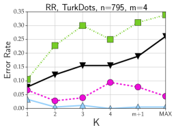
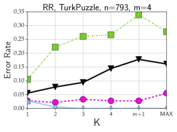
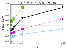
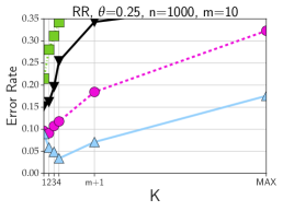
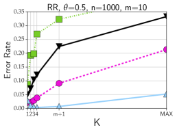
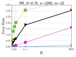
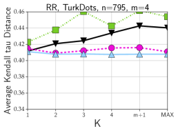
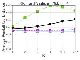
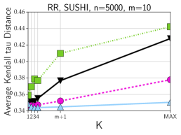
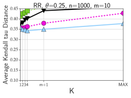
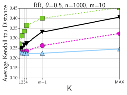
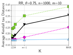
Figure 3: Performance of LDP-KwikSort:RR in terms of error rate and average Kendall tau distance on the real-world and synthetic datasets, across varying the number of queries $K$.

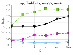
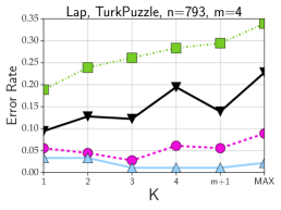
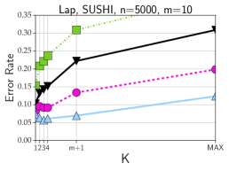
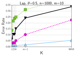
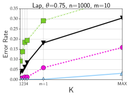
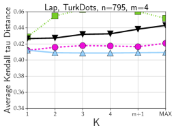
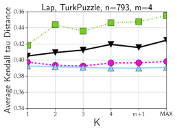
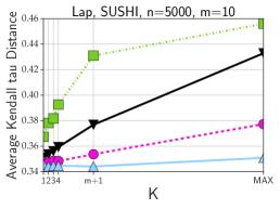
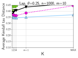
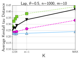
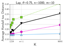
Figure 4: Performance of LDP-KwikSort:Lap in terms of error rate and average Kendall tau distance on the real-world and synthetic datasets, across varying the number of queries $K$.

6.3 The Impact of Privacy Budget

Next, we consider varying the privacy budget of each agent in the range $\{0.1,...,5.0\}$, and observe how this parameter impacts on the performance of LDP-KwikSort:RR and LDP-KwikSort:Lap under the utility metrics such as the error rate and the average Kendall tau distance. For the DP-KwikSort algorithm, as it is based on the local model of DP and the consumption of the privacy budget is originate from the curator, we also vary $\epsilon\in\{0.1,...,5.0\}$. In this experiment, we ran these two solutions of LDP-KwikSort and its competitors on three real-world datasets and three synthetic datasets. For the TurkDots, TurkPuzzle, and SUSHI datasets, the numbers of agents and alternatives are fixed by default. For the synthetic datasets, we set their dispersion parameter $\theta=0.25,0.5,0.75$, as well as $n=5000$ and $m=15$. The results are shown in Figure 5.

Firstly, the non-private KwikSort determines the overall lower error bound of average Kendall tau distance, and DP-KwikSort can approach it with a small privacy budget, say $\epsilon=0.1$. Secondly, with increasing the privacy budget, both of LDP-KwikSort:RR and LDP-KwikSort:Lap get lower errors, and the former outperforms the latter. Besides, the performance changing trends of solutions under two metrics are consistent, which is due to the error rate reflecting the accuracy of intermediate results while the average Kendall tau distance reflecting the utility of the aggregate ranking.

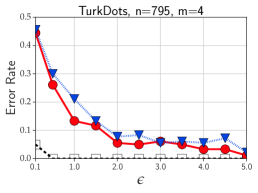
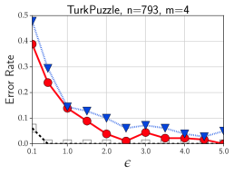
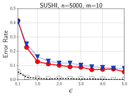
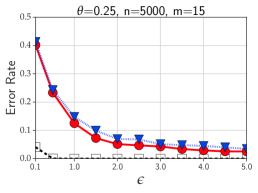
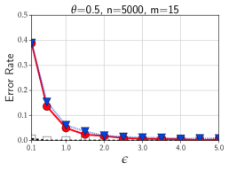
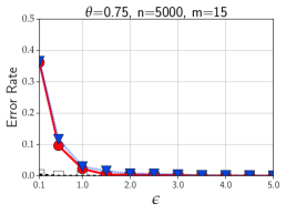
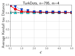
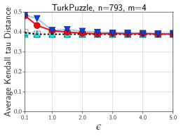
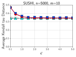
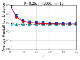
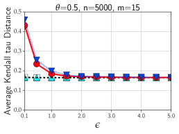
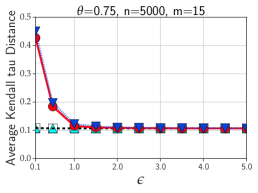
Figure 5: Comparison of protocols in terms of error rate and average Kendall tau distance on the real-world and synthetic datasets, across varying the privacy budget $\epsilon\in\{0.1,...5.0\}$.

6.4 The Impact of Agent and Alternative Amount

Intuitively, more alternatives that need to be ranked challenge the protocols for generating an optimal ranking. In order to maintain the results with an acceptable utility, the increase of the number of agents may help the curator to collect more information for rank aggregation. To investigate how the numbers of agents $n$ and alternatives $m$ impact on the performance, we ran these two solutions of LDP-KwikSort and its competitors on three real-world datasets and nine synthetic datasets, and consider to vary $n\in\{10,...,10000\}$ and $m\in\{4,10,15,30,45\}$, for observing the performance under the average Kendall tau distance. The results are shown in Figure 6.

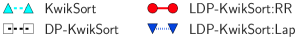
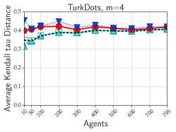
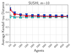
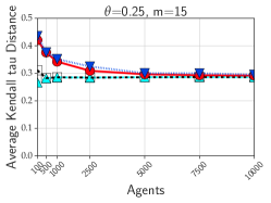
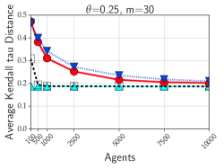
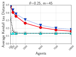
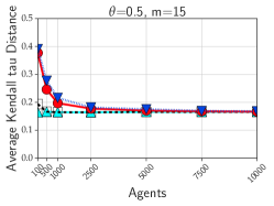
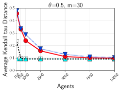
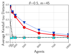
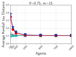
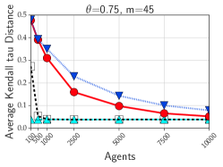
Figure 6: Comparison of protocols in terms of average Kendall tau distance on the real-world and synthetic datasets, across varying the number of agents $n$. Privacy budget $\epsilon$ is fixed at $2.0$.

In Figure 6-Figure 6, all the solutions are executed on the real-world datasets in which the number of alternatives are fixed by default and the privacy budget is set to $\epsilon=2.0$. Firstly, we observe that KwikSort algorithm still shows the lower error bound of the average Kendall tau distance. For instance, in Figure 6, with increasing the number of agents from $n=10$ to $n=100$, KwikSort can achieve the average Kendall tau distance below $0.4$ and get stable even with larger agent amount. And we further observe that when the number of agents is less than the number of possible pairs of alternatives $\binom{m}{2}$, KwikSort cannot aggregate a sufficient pairwise comparison profile in which each pairwise comparison $\texttt{cmp}_{\textbf{L}}(a_{j},a_{l})$ should be non-zero, which challenges the generation of optimal aggregate ranking. Secondly, the results show that LDP-KwikSort:RR still outperforms LDP-KwikSort:Lap. Generally, the involved solutions show the tendency of convergence as the increasing number of agents.

In Figure 6-Figure 6, we run all the solutions on the synthetic datasets with $\theta\in\{0.25,0.5,0.75\}$, varying the number of agents in a much larger range from $n=100$ to $n=10000$, and observe the performance of average Kendall tau distance under $m\in\{15,30,45\}$ and $\epsilon=2.0$. Firstly, the results show that with an increasing number of alternatives from $m=15$ to $m=45$, the lower error bound by KwikSort is decreasing, but it is much harder for the LDP-KwikSort protocol to achieve this bound unless given a large number of agents. For instance, when given $m=15$ alternatives, LDP-KwikSort:RR outperforms LDP-KwikSort:Lap by $8.1\%$ at $n=2500$, but with increasing $m$ to $30$, LDP-KwikSort:RR needs more agents, say $n=7500$, to achieve the improvement of $9.8\%$. Secondly, with increasing the number of alternatives, it will be more obvious to see the gap between LDP-KwikSort:RR and LDP-KwikSort:Lap. For instance, when setting $\theta=0.5$ and $n=2500$, their gaps at $m=15$, $m=30$ and $m=45$ are $2.4\%$, $11\%$ and $32.5\%$, respectively.

6.5 The Impact of Dispersion Parameter

In the above experiments, the dispersion parameters of synthetic dataset $\theta=0.25$, $\theta=0.5$ and $\theta=0.75$ are involved, which reflects the generated rankings are closer to the ground truth ranking. From the results in Figure 6, all solutions achieve lower average Kendall tau distance, which demonstrates the theoretical conclusions in Section 5.2. Besides, with increasing the dispersion parameter, it will be more obvious to see the gap between LDP-KwikSort:RR and LDP-KwikSort:Lap. For instance, when setting $m=45$ and $n=5000$, their gaps at $\theta=0.25$, $\theta=0.5$ and $\theta=0.75$ are $13.5\%$, $33.4\%$ and $46.5\%$, respectively.

6.6 Time Cost

Finally, we compare the time costs of all the solutions on three real-world datasets and five synthetic datasets. The results are shown in Table 3. We observe that KwikSort consumes the least execution time and the time increases with more alternatives because no noise introduced. On the basis of the former, the central model based DP-KwikSort algorithm shows a small increase in time cost. The cases of LDP-KwikSort protocol present the sum of the execution time of all the agents and the curator. We observe that when the number of alternatives are relatively small, say $m=4,5$, LDP-KwikSort:RR consumes less time than LDP-KwikSort:Lap. When increasing $m$ from $15$, LDP-KwikSort:RR needs more time cost.

Table 3: Comparison of protocols in terms of time cost (in seconds)

	TurkDots $795,4$	TurkPuzzle $793,4$	SUSHI $5000,10$	Mallows $5000,5$	Mallows $5000,10$	Mallows $5000,15$	Mallows $5000,30$	Mallows $5000,45$
KwikSort	0.0001	0.0001	0.0002	0.0001	0.0001	0.0002	0.0005	0.0007
DP-KwikSort	0.0006	0.0006	0.0030	0.0008	0.0030	0.0076	0.0285	0.0626
LDP-KwikSort:RR	0.1255	0.1244	2.7076	2.5783	2.6125	2.8551	3.3530	4.4113
LDP-KwikSort:Lap	0.1751	0.1732	2.9088	2.9015	2.9026	2.9294	2.9812	3.1288

6.7 Discussion

The above experimental results demonstrate that the proposed LDP-KwikSort can satisfy $\epsilon$-local differential privacy or $\epsilon$-local individual differential privacy while maintaining the acceptable utility of the aggregate ranking. Particularly, under the utility metrics such as the error rate and the average Kendall tau distance, solution LDP-KwikSort:RR generally outperforms LDP-KwikSort:Lap and can achieve the closest performance of DP-KwikSort. When using the proposed protocol in an agent scale as $n=5000$, we recommend $\epsilon=1.0$ for the situations with fewer alternatives such as $m\leq 15$, and $\epsilon=3.0$ when considering a relatively large number of alternatives.

Due to the natural shortcoming of the local model of DP, the observed limitation of this work relies on the relatively large privacy budget to maintain the acceptable utility, compare with that of central model based solutions. The potential optimization methods include the consideration of personalized privacy settings.

7 Conclusion

Rank aggregation aims to combine different agents’ preferences over the given alternatives into an aggregate ranking that agrees with the most with all the preferences. In the scenario of crowdsourced data management, since the aggregation procedure relies on a data curator, the privacy within the agents’ preference data could be compromised when the curator is untrusted. All existing works that guarantee differential privacy in rank aggregation assume that the data curator is trusted.

This paper first formalizes and studies the locally differentially private rank aggregation (LDP-RA) problem. Specifically, we design the LDP-KwikSort protocol which could protect the pairwise comparison within the ranking list. It also shows a combination of the properties from the approximate rank aggregation algorithm KwikSort, the RR mechanism, and the Laplace mechanism. Theoretical analysis and empirical results on the real-world and synthetic datasets confirm that our protocol especially the solution LDP-KwikSort:RR can achieve strong local privacy protection while maintaining an acceptable utility.

Future work will include the following three aspects: 1) considering strategic voting behaviors and exploring the trade-off between the soundness, the usefulness and the privacy preservation in LDP-RA; 2) extending our approach to support personalized privacy budget setting for different agents; 3) the evaluation of the synthetic rank datasets based on other mixture models such as the Plackett-Luce model and the general random utility model.

References

- Ailon et al. [2005] Nir Ailon, Moses Charikar, and Alantha Newman. Aggregating inconsistent information: ranking and clustering. In STOC, pages 684–693. ACM, 2005.
- Ailon et al. [2008] Nir Ailon, Moses Charikar, and Alantha Newman. Aggregating inconsistent information: Ranking and clustering. J. ACM, 55(5):23:1–23:27, 2008.
- Baker et al. [2016] Melissa A Baker, Paul Fox, and T Wingrove. Crowdsourcing as a forensic psychology research tool. American Journal of Forensic Psychology, 34(1):37–50, 2016.
- Bassily et al. [2017] Raef Bassily, Kobbi Nissim, Uri Stemmer, and Abhradeep Guha Thakurta. Practical locally private heavy hitters. In NIPS, pages 2285–2293, 2017.
- Bates and Lanza [2013] John A Bates and Brian A Lanza. Conducting psychology student research via the mechanical turk crowdsourcing service. North American Journal of Psychology, 15(2), 2013.
- Behrend et al. [2011] Tara S Behrend, David J Sharek, Adam W Meade, and Eric N Wiebe. The viability of crowdsourcing for survey research. Behavior Research Methods, 43(3):800, 2011.
- Beliakov et al. [2016] Gleb Beliakov, Humberto Bustince Sola, and Tomasa Calvo. A Practical Guide to Averaging Functions, volume 329 of Studies in Fuzziness and Soft Computing. Springer, 2016.
- Brancotte et al. [2015] Bryan Brancotte, Bo Yang, Guillaume Blin, Sarah Cohen Boulakia, Alain Denise, and Sylvie Hamel. Rank aggregation with ties: Experiments and analysis. PVLDB, 8(11):1202–1213, 2015.
- Brandt et al. [2016] Felix Brandt, Vincent Conitzer, Ulle Endriss, Jérôme Lang, and Ariel D. Procaccia, editors. Handbook of Computational Social Choice. Cambridge University Press, 2016.
- Chaudhuri [2016] Arijit Chaudhuri. Randomized Response and Indirect Questioning Techniques in Surveys. Chapman and Hall/CRC, 2016.
- Chen et al. [2013] Yiling Chen, Stephen Chong, Ian A. Kash, Tal Moran, and Salil P. Vadhan. Truthful mechanisms for agents that value privacy. In EC, pages 215–232. ACM, 2013.
- Chen et al. [2016] Yiling Chen, Stephen Chong, Ian A. Kash, Tal Moran, and Salil P. Vadhan. Truthful mechanisms for agents that value privacy. ACM Trans. Economics and Comput., 4(3):13:1–13:30, 2016.
- Cortes [2017] David Cortes. Ordering lists based on aggregated pairwise preferences, 2017. https://pypi.org/project/pwlistorder/.
- Duchi et al. [2012] John C. Duchi, Michael I. Jordan, and Martin J. Wainwright. Privacy aware learning. In NIPS, pages 1439–1447, 2012.
- Duchi et al. [2013] John C. Duchi, Michael I. Jordan, and Martin J. Wainwright. Local privacy and statistical minimax rates. In FOCS, pages 429–438. IEEE Computer Society, 2013.
- Dwork [2006] Cynthia Dwork. Differential privacy. In ICALP (2), volume 4052 of Lecture Notes in Computer Science, pages 1–12. Springer, 2006.
- Dwork and Roth [2014] Cynthia Dwork and Aaron Roth. The algorithmic foundations of differential privacy. Foundations and Trends in Theoretical Computer Science, 9(3-4):211–407, 2014.
- Eppstein [2015] David Eppstein. Instability vs anonymization in e pluribus hugo, 2015. https://11011110.github.io/blog/2015/09/09/instability-vs-anonymization.html.
- Greenberg et al. [1969] Bernard G. Greenberg, Abdel-Latif A. Abul-Ela, Walt R. Simmons, and Daniel G. Horvitz. The unrelated question randomized response model: Theoretical framework. Journal of the American Statistical Association, 64(326):520–539, 1969.
- Groat et al. [2013] Michael M. Groat, Benjamin Edwards, James Horey, Wenbo He, and Stephanie Forrest. Application and analysis of multidimensional negative surveys in participatory sensing applications. Pervasive and Mobile Computing, 9(3):372–391, 2013.
- Hay et al. [2017] Michael Hay, Liudmila Elagina, and Gerome Miklau. Differentially private rank aggregation. In SDM, pages 669–677. SIAM, 2017.
- Holohan et al. [2017] Naoise Holohan, Douglas J. Leith, and Oliver Mason. Optimal differentially private mechanisms for randomised response. IEEE Trans. Information Forensics and Security, 12(11):2726–2735, 2017.
- Huang and Du [2008] Zhengli Huang and Wenliang Du. Optrr: Optimizing randomized response schemes for privacy-preserving data mining. In ICDE, pages 705–714. IEEE Computer Society, 2008.
- Irurozki et al. [2016] Ekhine Irurozki, Borja Calvo, and Jose A. Lozano. Permallows: An r package for mallows and generalized mallows models. Journal of Statistical Software, 71(i12), 2016.
- Kamishima [2003] Toshihiro Kamishima. Nantonac collaborative filtering: recommendation based on order responses. In KDD, pages 583–588. ACM, 2003.
- Kang et al. [2014] Ruogu Kang, Stephanie Brown, Laura Dabbish, and Sara B. Kiesler. Privacy attitudes of mechanical turk workers and the U.S. public. In SOUPS, pages 37–49. USENIX Association, 2014.
- Kasiviswanathan et al. [2008] Shiva Prasad Kasiviswanathan, Homin K. Lee, Kobbi Nissim, Sofya Raskhodnikova, and Adam D. Smith. What can we learn privately? In FOCS, pages 531–540. IEEE Computer Society, 2008.
- Lease et al. [2013] Matthew Lease, Jessica Hullman, Jeffrey Bigham, Michael Bernstein, Juho Kim, Walter Lasecki, Saeideh Bakhshi, Tanushree Mitra, and Robert Miller. Mechanical turk is not anonymous. Available at SSRN 2228728, 2013.
- Lee [2015] David Timothy Lee. Efficient, private, and eps-strategyproof elicitation of tournament voting rules. In IJCAI, pages 2026–2032. AAAI Press, 2015.
- Li et al. [2016a] Guoliang Li, Jiannan Wang, Yudian Zheng, and Michael J. Franklin. Crowdsourced data management: A survey. IEEE Trans. Knowl. Data Eng., 28(9):2296–2319, 2016a.
- Li et al. [2016b] Ninghui Li, Min Lyu, Dong Su, and Weining Yang. Differential Privacy: From Theory to Practice. Synthesis Lectures on Information Security, Privacy, & Trust. Morgan & Claypool Publishers, 2016b.
- Li et al. [2018a] Yaliang Li, Chenglin Miao, Lu Su, Jing Gao, Qi Li, Bolin Ding, Zhan Qin, and Kui Ren. An efficient two-layer mechanism for privacy-preserving truth discovery. In KDD, pages 1705–1714. ACM, 2018a.
- Li et al. [2018b] Yaliang Li, Houping Xiao, Zhan Qin, Chenglin Miao, Lu Su, Jing Gao, Kui Ren, and Bolin Ding. Towards differentially private truth discovery for crowd sensing systems. CoRR, abs/1810.04760, 2018b.
- Liu et al. [2018] Ao Liu, Yun Lu, Lirong Xia, and Vassilis Zikas. How private is your voting? A framework for comparing the privacy of voting mechanisms. CoRR, abs/1805.05750, 2018.
- Mallows [1957] Colin L Mallows. Non-null ranking models. Biometrika, 44(1/2):114–130, 1957.
- Mao et al. [2013] Andrew Mao, Ariel D. Procaccia, and Yiling Chen. Better human computation through principled voting. In AAAI. AAAI Press, 2013.
- Miller et al. [2017] Joshua D Miller, Michael Crowe, Brandon Weiss, Jessica L Maples-Keller, and Donald R Lynam. Using online, crowdsourcing platforms for data collection in personality disorder research: The example of amazon s mechanical turk. Personality Disorders: Theory, Research, and Treatment, 8(1):26, 2017.
- Nissim et al. [2007] Kobbi Nissim, Sofya Raskhodnikova, and Adam D. Smith. Smooth sensitivity and sampling in private data analysis. In STOC, pages 75–84. ACM, 2007.
- Peer et al. [2017] Eyal Peer, Laura Brandimarte, Sonam Samat, and Alessandro Acquisti. Beyond the turk: Alternative platforms for crowdsourcing behavioral research. Journal of Experimental Social Psychology, 70:153–163, 2017.
- Peng et al. [2018] Kaiping Peng, Shiqun Liu, and Shiguang Ni. Amazon mechanical turk crowdsourcing: A research tool in mobile internet era. Journal of Northwest Normal University (Social Sciences), v.55 No.259(3):115–125, 2018.
- Sannon and Cosley [2018] Shruti Sannon and Dan Cosley. ”it was a shady hit”: Navigating work-related privacy concerns on mturk. In CHI Extended Abstracts. ACM, 2018.
- Sei and Ohsuga [2017] Yuichi Sei and Akihiko Ohsuga. Differential private data collection and analysis based on randomized multiple dummies for untrusted mobile crowdsensing. IEEE Trans. Information Forensics and Security, 12(4):926–939, 2017.
- Shang et al. [2014] Shang Shang, Tiance Wang, Paul Cuff, and Sanjeev R. Kulkarni. The application of differential privacy for rank aggregation: Privacy and accuracy. In FUSION, pages 1–7. IEEE, 2014.
- Shank [2016] Daniel B Shank. Using crowdsourcing websites for sociological research: The case of amazon mechanical turk. The American Sociologist, 47(1):47–55, 2016.
- Soria-Comas et al. [2017] Jordi Soria-Comas, Josep Domingo-Ferrer, David Sánchez, and David Megías. Individual differential privacy: A utility-preserving formulation of differential privacy guarantees. IEEE Trans. Information Forensics and Security, 12(6):1418–1429, 2017.
- Wang et al. [2019] Shaowei Wang, Jiachun Du, Wei Yang, Xinrong Diao, Zichun Liu, Yiwen Nie, Liusheng Huang, and Hongli Xu. Aggregating votes with local differential privacy: Usefulness, soundness vs. indistinguishability. CoRR, abs/1908.04920, 2019.
- Wang et al. [2017] Tianhao Wang, Jeremiah Blocki, Ninghui Li, and Somesh Jha. Locally differentially private protocols for frequency estimation. In USENIX Security Symposium, pages 729–745. USENIX Association, 2017.
- Wang et al. [2016] Yue Wang, Xintao Wu, and Donghui Hu. Using randomized response for differential privacy preserving data collection. In EDBT/ICDT Workshops, volume 1558 of CEUR Workshop Proceedings. CEUR-WS.org, 2016.
- Warner [1965] Stanley L. Warner. Randomized response: A survey technique for eliminating evasive answer bias. Journal of the American Statistical Association, 60(309):63–69, 1965.
- Wikipedia [2019] Wikipedia. Hoeffding’s inequality, 2019. https://en.wikipedia.org/wiki/Hoeffding’s_inequality.
- Xia et al. [2017] Huichuan Xia, Yang Wang, Yun Huang, and Anuj Shah. ”our privacy needs to be protected at all costs”: Crowd workers’ privacy experiences on amazon mechanical turk. PACMHCI, 1(CSCW):113:1–113:22, 2017.
- Yan et al. [2019] Ziqi Yan, Jiqiang Liu, and Shaowu Liu. Dpwevote: Differentially private weighted voting protocol for cloud-based decision-making. Enterprise IS, 13(2):236–256, 2019.
- Zhu et al. [2017a] Tianqing Zhu, Gang Li, Wanlei Zhou, and Philip S. Yu. Differentially private data publishing and analysis: A survey. IEEE Trans. Knowl. Data Eng., 29(8):1619–1638, 2017a.
- Zhu et al. [2017b] Tianqing Zhu, Gang Li, Wanlei Zhou, and Philip S. Yu. Differential Privacy and Applications, volume 69 of Advances in Information Security. Springer, 2017b.