Hidden-charm pentaquarks with color-octet substructure in QCD Sum Rules

Abstract

We study the hidden-charm pentaquark states $udsc\bar{c}$ with spins 1/2, 3/2, and 5/2 within the QCD sum-rule approach. First, we construct the currents for the particular configuration of pentaquark states that consist of the flavor singlet three-quark cluster $uds$ of spins 1/2 and 3/2 and the two-quark cluster $\bar{c}c$ of spin 1, where both clusters are in a color-octet state. From the QCD sum rules obtained by the operator product expansion up to dimension-10 condensates, the extracted masses for the pentaquark states $uds$-$\bar{c}c$ are about 4.6 GeV (5.6 GeV) for spin 1/2^±, about 5.1 GeV (6.0 GeV) for spin 3/2^±, about 6.1 GeV (5.9 GeV) for spin 5/2^±, where the masses of the positive parity states are given in parentheses. Additionally, based on the flavor singlet pentaquark states, it is also shown that other pentaquark states of clusters like $udc$-$\bar{c}s$ and $usc$-$\bar{c}d$ lead to masses similar to the $uds$-$\bar{c}c$ case within error bars. Furthermore, in order to see whether any of the states, observed by the LHCb Collaboration, could be understood as the pentaquark of two clusters in the color-octet state, we study the pentaquark formed by the two clusters $udc$-$\bar{c}u$, where the three-quark cluster is assumed to have the same flavor structure as the above $uds$ cluster. We come to the conclusion that if the observed pentaquark will be found to have spin 1/2 and negative parity, then it could be described as a state of two color-octet clusters.

I Introduction

Since the observation of the two exotic hidden-charm pentaquark $P_{c}^{+}$ states of the quark content $uudc\bar{c}$ with the spins 3/2 and 5/2 through the decay $\Lambda_{b}^{0}\rightarrow J/\psi K^{-}p$ by LHCb collaboration Aaij:2015tga , many studies on these states and other expected hidden-charm pentaquark states have been performed. Note that recently the LHCb collaboration has observed a three peak structure Aaij:2019vzc ; Cao:2019kst using an updated analysis. There is an intriguing possibility Cao:2019gqo ; Wang:2019krd that pentaquark states could be observed on Electron-Ion Collider China (EicC). The pentaquark states, including the above hidden-charm pentaquark states, have been theoretically studied using quark models Wu:2017weo ; Santopinto:2016pkp ; Irie:2017qai , diquark models and triquark-diquark models Maiani:2015vwa ; Lebed:2015tna ; Li:2015gta ; Zhu:2015bba ; Wang:2015epa ; Jaffe:2003sg ; Sugiyama:2003zk ; Lee:2005ny ; Karliner:2003dt ; Zhu:2003ba , hadronic molecular states Chen:2015moa ; Roca:2015dva ; He:2015cea ; Azizi:2016dhy ; Guo:2017jvc , the coupled-channel unitary approach Wu:2010jy ; Wu:2010vk ; Shen:2019evi , the contact-range effective field theory Liu:2019tjn , and the hadroquarkonia model Eides:2017xnt . For a review on the hidden-charm multiquark states, see Chen:2016qju . Among the expected hidden-charm pentaquark states, it is very intriguing to analyze the pentaquark state of the quark content $udsc\bar{c}$ since $\Lambda_{b}^{0}$ could also decay into $J/\psi K^{-}p$ via $J/\psi\Lambda^{*}$ and such pentaquark state could be observed through the decay $\Xi^{-}_{b}\rightarrow J/\psi\Lambda K^{-}$ Santopinto:2016pkp .

Most of the models and approaches to the pentaquark states in the references discussed above rely on an assumption that a pentaquark state under consideration has certain structure in color, spin, and flavor. Considering the interpolating current to a pentaquark state for analysis within the QCD sum-rules (SRs), the clustering in the color, flavor and spin space is inevitable due to the absence of the invariant rank-5 tensors for the color, flavor and spin subspaces. For example for $SU(3)_{c}$, the largest rank of invariant tensor is 3, therefore considering two-quarks and three-quarks cluster would be one of the natural possibilities in constructing the interpolating for a pentaquark state. Recently, the hidden-charm pentaquark state of the quark content $udsc\bar{c}$ with the flavor singlet structure in $SU_{F}(3)$ (the flavor singlet hidden-charm pentaquark) was considered in Irie:2017qai within quarks models. Specially, the flavor singlet hidden-charm pentaquark was analyzed as the bound state of a three-quark and two-quark parts both in color octets, and the stable result was got for the total spin 1/2 in Irie:2017qai .

In this paper, we study first the flavor singlet hidden-charm pentaquark states of $udsc{\bar{c}}$ with the spins $1/2$, $3/2$, and $5/2$ using QCD SRs. We assume that these states consist of two colored clusters as discussed in Mironov:2015ica ; Irie:2017qai ; Takeuchi:2016ejt within quark models. So, we consider them as states consisting of the three-quark cluster $uds$ and the two-quark cluster ${\bar{c}}c$. Additionally, we assume that all quarks are in an $S$-wave, the colors of both clusters are color octets, and the two-quark cluster has spin 1 since it has been shown in Irie:2017qai that such clusters of $uds$ and ${\bar{c}}c$ yielded the most stable result. To check this assumption, we consider the pentaquark states containing a scalar two-quark cluster and find that such states lead to higher masses than those obtained from pentaquarks with a two-quark cluster of spin 1. Then, we also examine other possible pentaquark states containing the two clusters $udc$-${\bar{c}}s$ and $usc$-${\bar{c}}d$ by extending the results of the flavor singlet $uds$ and ${\bar{c}}c$ case. Furthermore, the pentaquark states of the two color-octet clusters $udc$-${\bar{c}}u$ are studied to see if any of the states observed by LHCb could be understood in terms of pentaquark state with color-octet substructure and flavor-singlet flavor three-quark part $udc$. Let us point out that the method of QCD SR relies on the local current for studying the spectroscopy of hadrons. In this work, therefore, we construct only the local currents for pentaquark in the configuration space with all quarks located at the same point. The particular configuration and clustering reflect the properties only in flavor, color and spin subspaces.

This paper is organized as follows. Using the above assumptions, we construct in Sec. II the interpolating currents for the hidden-charm pentaquark states with spins 1/2, 3/2, and 5/2 in the form of a product of the currents for these two clusters as

$$J_{\text{5q}}=J_{3q}^{m}\,J_{2q}^{m}\,$$

with the color index $m$. We perform the operator product expansion (OPE) for the correlators with the interpolating currents in Sec. III and present the system of the employed QCD sum rules in Sec. IV. Furthermore, since the relativistic interpolating currents for the fermions can be coupled to the two states with opposite parities when the QCD sum rules are constructed, we discuss how to extract the contribution to a state with definite parity from the system of the QCD sum rules in Sec. IV. Finally, a comprehensive discussion of the results is given in Sec. V.

II Interpolating Currents

First, we consider the wave function of the flavor singlet $uds$ cluster for constructing the three-quark interpolating current $J_{3q}^{m}$. Then, we extend our current to the case of three arbitrary flavors. We will take the flavor structure of the interpolating current $J_{3q}^{m}$ from the flavor singlet wave function in the flavor $SU(3)$ space as

$$J_{\text{flavor}}\sim(ud-du)s+(su-us)d+(ds-sd)u\,.$$ (1)

We study both cases of an $uds$ cluster: one with spin 1/2 and one with spin 3/2 for a total spin 1/2, 3/2, and 5/2 of the pentaquark states. To this end, we adopt the QCD SR method applied to the analysis of the baryon octet Ioffe:1981kw . Therefore, we construct the current with the first two quarks contributing spin 0 to the total spin of the three-quark cluster with spin 1/2. On the other hand, in the current for the three-quark cluster with spin 3/2, the first two quarks give spin 1 to the total spin.

With these ingredients and Ioffe’s current Ioffe:1981kw ; Ioffe:2010zz with the definite chiralities which are well known to form a good basis, we consider the following structure of the spin part of the interpolating current of the three-quark cluster with spin 1/2

$$J_{\text{spin}}^{\text{A}}\! = \!4(u^{T}_{R}C\Gamma_{\text{A}}d_{R})\Gamma_{2}s_{L}-(R\leftrightarrow L)$$

$$= (u^{T}C\{\gamma_{5},\Gamma_{\text{A}}\}d)\Gamma_{2}s-(u^{T}C\{\gamma_{5},\Gamma_{\text{A}}\}\gamma_{5}d)\Gamma_{2}\gamma_{5}s\,,$$

where the superscript A means that the current is antisymmetric under the exchange of the spinor indexes of the first two quarks. The first term in Eq. (1) is considered as an example, and then the rest is included in the final stage. From the above expression, $\Gamma_{\text{A}}$ must satisfy the following conditions in order to have no zero current

$$\{\gamma_{5},\Gamma_{\text{A}}\}\neq 0\ ,\ (C\Gamma_{\text{A}})^{T}=-C\Gamma_{\text{A}}\,,$$

where $T$ means the transposition. These conditions limit the choices of $\Gamma_{\text{A}}$ to $\Gamma_{\text{A}}=1,\ \gamma_{5}$. For a $uds$ cluster of spin 3/2, we consider

$$J_{\text{spin}}^{\text{S}}\! = \!2(u^{T}_{R}C\Gamma_{\text{S}}d_{L})\Gamma_{2}\gamma_{5}s+(R\leftrightarrow L)$$

$$= (u^{T}C[\Gamma_{\text{S}},\gamma_{5}]\gamma_{5}d)\Gamma_{2}\gamma_{5}s\,$$

where the superscript S denotes that the current is symmetric under the exchange of the spinor indexes of the first two quarks. Similarly to the case of the above current for the spin 1/2 case, $\Gamma_{\text{S}}$ must satisfy the following conditions

$$[\gamma_{5},\Gamma_{\text{S}}]\neq 0,\ (C\Gamma_{\text{S}})^{T}=C\Gamma_{\text{S}}\,.$$

in order to have a nonzero current. Therefore, the only choice is $\Gamma_{\text{S}}=\gamma_{\mu}$.

Before constructing the full current, we study the currents in color subspace. Using the adjoint representation of color $SU(3)$, the color-octet structure of the current can be constructed as

$$J_{\text{color}}^{\text{S/A}}=\epsilon_{ac\omega}t^{m}_{\omega b}~{}u_{a}d_{b}s_{c}\,,$$

where $m$ is a color index. Other choices for color tensors lead to zero currents or to the same full currents due to the symmetries in the spin and flavor subspaces.

To generalize the $uds$ case, considered above, to other flavors of three-quark clusters, we distinguish the quarks in the three-quark cluster by $(q_{1},q_{2},q_{3})$. Combining the currents constructed in the flavor, spin and color subspaces, we get the interpolating currents for the considered structure of pentaquark states in the form of

$$J_{l}^{\text{A}}(\Gamma_{2}\,,\Gamma_{3})=T_{l,m}^{\text{A}}(\Gamma_{2})q^{T}_{1}q_{2}q_{3}(\bar{q}_{5}t^{m}\Gamma_{3}q_{4})\,,$$ (4)

$$J_{\mu,l}^{\text{S}}(\Gamma_{2}\,,\Gamma_{3})=T_{\mu,l,m}^{\text{S}}(\Gamma_{2})q^{T}_{1}q_{2}q_{3}(\bar{q}_{5}t^{m}\Gamma_{3}q_{4})\,.$$

Here, the quark fields in the three-quark cluster carry flavor $f_{i}$, color $c_{i}$ and spin $l_{i}$ indices as $q_{i}=q_{f_{i}c_{i}l_{i}}$ to be contracted with the tensor which becomes

$$T^{\text{A}}_{l,m}(\Gamma_{2}) = \large(C_{l_{1}l_{2}}(\Gamma_{2})_{ll_{3}}-(C\gamma_{5})_{l_{1}l_{2}}(\gamma_{5}\Gamma_{2})_{ll_{3}}\large)$$

$$\times\epsilon_{f_{1}f_{2}f_{3}}\epsilon_{c_{1}c_{3}c}t^{m}_{cc_{2}}\,,$$

$$T^{\text{S}}_{\mu,l,m}(\Gamma_{2}) = \large(C\gamma_{\mu}\large)_{l_{1}l_{2}}\large(\Gamma_{2}\large)_{ll_{3}}\epsilon_{f_{1}f_{2}f_{3}}\epsilon_{c_{1}c_{3}c}t^{m}_{cc_{2}}\,.$$

These definitions reflect our choice for $\Gamma_{\text{A}}=\gamma_{5}$ and $\Gamma_{\text{S}}=\gamma_{\mu}$. We denote the flavor configuration by $q^{1}q^{2}q^{3}\text{-}\bar{q}^{5}q^{4}$, where $q^{i}$ is the flavor of the $i$-th quark $q_{i}$. In this work, as mentioned in the introduction, we consider four cases for a given flavor configuration: $uds$-$\bar{c}c$ ,  $udc$-$\bar{c}s$ ,  $usc$-$\bar{c}d$ and $udc$-$\bar{c}u$. Quarks fields are contracted with the antisymmetric tensor of flavor indices that corresponds to the flavor singlet configuration. Note that the free index $l$ denotes the spinor component of the current and will be omitted in the following discussion.

We mention here again that the spinor structure of the three-quark cluster in the full current Eq. (4) is chosen to have the particular structure of $q_{R}q_{R}q_{L}-q_{L}q_{L}q_{R}$ for the antisymmetric case, Eq. (II), and $q_{R}q_{L}q+q_{L}q_{R}q$ for the symmetric case Eq. (II).

The matrix $\Gamma_{2}$, which can be considered as a factor of the current due to the following properties

$$J^{\text{S/A}}_{l}(\Gamma_{2}\,,\Gamma_{3})=(\Gamma_{2})_{lk}J^{\text{S/A}}_{k}(1,\Gamma_{3})\,,$$

will be chosen according to the P-parity and the spin of the interpolating current under consideration. As for $\Gamma_{3}$, following the analysis of Irie:2017qai , where the two-quark cluster with spin 1 in the $uds$-${\bar{c}}c$ system yielded the most stable result, we will take $\Gamma_{3}=\gamma_{\nu}$ for most pentaquark states considered in this work. An alternative option for $\Gamma_{3}=1$ will also be considered.

To discuss the symmetry properties of the constructed three-quark currents in the color-spin subspace, we consider the six-dimensional fundamental representation of the $SU(6)$ group  Gursey:1992dc ; bookCloseQuarks composed of the tensor product of the color $SU(3)_{\rm color}$ and the spin $SU(2)_{\rm spin}$ subgroups. Representing a quark by its dimension $(3,2)$ where the first (second) corresponds to the dimension of $SU(3)_{\rm color}$ ($SU(2)_{\rm spin}$) subgroup, we have

$$\!\!(3,2)\!\otimes\!(3,2)\!\otimes\!(3,2)=(8,2)\!\oplus\!(8,4)\!\oplus\cdots\,,$$

where only two irreducible representations are shown. The first term on the right-hand side has spin 1/2 and belongs to the fully symmetric 56-plet representation, while the second term has spin 3/2 and belongs to the mixed symmetric 76-plet of the full $SU(6)$ group. The color-spin part of the constructed current $J^{\text{A}}$, Eq. (4), represents (8,2) states studied in Irie:2017qai . The current $J^{\text{S}}$ corresponds to (8,2) and (8,4), depending on the choice of $\Gamma_{2}$.

In this section, we have constructed the general form for the pentaquark currents $J_{8}\sim qqq$-$\bar{q}q$ with two color-octet compounds. The suggested currents are unique and can’t be presented by the sum of any other currents considered previously. Nevertheless, omitting the flavor structure, we have related this type of current with another types of currents that represent following configurations in color subspace: diquark-diquark-antiquark clustering $J_{\bar{3}}\sim qq$-$qq$-$\bar{q}$ with an anti-triplet color substructure suggested in Jaffe:2003sg ; Sugiyama:2003zk ; Lee:2005ny , and a molecule form $J_{1}\sim qqq$-$\bar{q}q$ with color-singlet parts, see Guo:2017jvc . We conclude, that for any current of color-octet type $J_{8}$, one can find two specific (in spin and isospin) currents of color-singlet type $J_{1}$ and color-anti-triplet type $J_{\bar{3}}$ such that $J_{8}=J_{1}+J_{\bar{3}}$. For more details see Appendix C, where we show how to construct these specific currents in spin space.

III OPE for $1/2$, $3/2$, $5/2$-states

The correlator $\Pi^{s}_{(\mu)(\nu)}(q^{2})$ for the QCD sum-rule analysis of a pentaquark state is defined by

$$\Pi^{s}_{(\mu)(\nu)}(q^{2})=i\int d^{4}xe^{iq\cdot x}\langle 0|TJ_{(\mu)}(x)\bar{J}_{(\nu)}(0)|0\rangle$$ (5)

with the interpolating current $J_{(\mu)}$ for the considered pentaquark state of spin $s$. The subscript $(\mu)$ stands for the possible Lorentz indices of currents for the $s=3/2,~{}5/2$ states. Since the current $J_{(\mu)}$ can couple to the states with a spin lower than $s$, the phenomenological part of the SRs contains contributions from the lower spin states as well. Extracting the contribution from the state with spin $s$ only, the correlator can be written as

$$\Pi^{s}_{(\mu)(\nu)}(q^{2})=(\hat{q}\Pi^{s}_{1}(q^{2})+\Pi^{s}_{2}(q^{2}))S^{s}_{(\mu)(\nu)}+\cdots\,,$$ (6)

where $\hat{q}=\gamma\cdot q$ and $\cdots$ means the terms corresponding to the omitted contributions from states with spin $s$ and also lower spins. Therefore, to construct SRs for the state of spin $s$, one needs to extract $\Pi^{s}_{1,2}$ from the correlator. The ways of extracting $\Pi^{s}_{1,2}$ for $s=3/2,~{}5/2$ are summarized in Appendices A and B. Then, QCD SRs for the state of the spin $s$ will be constructed by applying the dispersion relation Shifman:1978bx to the two scalar functions $\Pi^{s}_{1,2}$ in Eq. (6)

$$\Pi^{s}_{i}(q^{2})=\int_{s_{\text{th}}}^{\infty}dt\frac{\rho^{s}_{i}(t)}{t-q^{2}}\,.$$ (7)

Here the spectral densities $\rho^{s}_{i}(t)$ are defined in the physical $t$ region by

$$\rho^{s}_{i}(t)=\frac{1}{\pi}\text{Im}\Pi^{s}_{i}(t)$$ (8)

with $i=1,2$.

In the next subsections A, B, C, we present the relativistic interpolating currents for each state of spin 1/2, 3/2, and 5/2 states with proper choices of $\Gamma_{1}$, $\Gamma_{2}$, and $\Gamma_{3}$. Then, in subsection D, we show how to calculate the spectral densities $\rho^{s}_{i}(t)$ within the OPE for the QCD sum rules for each state.

III.1 $J^{P}=1/2^{\pm}$-states

We consider four types of the current for the spin 1/2 case:

$$J^{1}=J^{\text{A}}(\gamma_{5}\gamma_{\mu}\,,\gamma_{\mu})\,,~{}~{}J^{2}=J^{\text{S}}_{\mu}(\gamma_{5}\,,\gamma_{\mu})\,,$$ (9)

$$J^{3}=J^{\text{A}}(\gamma_{5}\,,1)\,,~{}~{}J^{4}=J^{\text{S}}_{\mu}(\gamma_{5}\gamma_{\mu}\,,1)\,,$$

where the upper index denotes the type of the current. The main results for the spin 1/2 case are obtained using the current $J^{1}$, while currents $J^{2}$, $J^{3}$, $J^{4}$ are also studied as an alternative option. The interpolating current $J^{1}$ with the quantum numbers $1/2^{+}$ can be related to the spin-3/2 current as follows

$$J^{1}=J^{\text{A}}(\gamma_{5}\gamma_{\mu}\,,\gamma_{\mu})=-\gamma_{\mu}J^{1}_{\mu}\,.$$

The choice of $\Gamma_{2}=\gamma_{5}\gamma_{\mu}$ insures that the spin-3/2 current $J_{\mu}$ is projected by $\Gamma_{2}$ only on the 1/2-spin component so that $\langle{0|\gamma_{\mu}J_{\mu}|3/2^{\pm}}\rangle\sim\gamma_{\mu}u_{\mu}=0$ thanks to the subsidiary condition for the 3/2 spinor $u_{\mu}$ (see Eqs. (11) and (12)). Since the relativistic interpolating current is considered, as discussed in Chung:1981cc ; Jido:1996ia , the current can couple to the state of negative parity as well. Denoting two such states by $|1/2^{+}\rangle$ and $|1/2^{-}\rangle$, the current couples to the states through the following relations

$$\langle{0|J|1/2^{+}}\rangle = f_{\frac{1}{2}+}u\,,~{}~{}~{}\langle{0|J|1/2^{-}}\rangle=f_{\frac{1}{2}-}\gamma_{5}u\,,$$

$$\sum\limits_{s}u(q,s)\bar{u}(q,s) = \hat{q}+m\$$ (10)

with the spinor $u$. The structure of the correlator becomes

$$\Pi^{1/2}(q^{2}) = \hat{q}\Pi^{1/2}_{1}(q^{2})+\Pi^{1/2}_{2}(q^{2})$$

and then $S^{1/2}_{(\mu)(\nu)}=1$ because there is no Lorentz index in the current. The two spectral densities can be obtained as

$$\rho_{1}^{1/2}(s) = \frac{1}{4\pi s}{\rm Tr}\bigg{(}\hat{q}\textbf{Im}\Pi^{1/2}(s)\bigg{)}\ ,$$

$$\rho_{2}^{1/2}(s) = \frac{1}{4\pi}{\rm Tr}\bigg{(}\textbf{Im}\Pi^{1/2}(s)\bigg{)}\ .$$

III.2 $3/2^{\pm}$-states

For spin 3/2 states , we study two types of the current

$$J^{1}_{\mu}=J^{\text{A}}(\gamma_{5}\,,\gamma_{\mu})\,,~{}~{}J^{2}_{\mu}=J^{\text{S}}_{\mu}(\gamma_{5}\,,1)\,.$$ (11)

The main results will be obtained by using the current $J^{1}_{\mu}$ that has the quantum numbers $3/2^{-}$. As in the spin-1/2 case, the interpolating current couples to the states of both parities through the relations with the corresponding spinors $u_{\mu}$ Azizi:2016dhy ; Wang:2015epa

$$\langle{0|J_{\mu}|3/2^{+}}\rangle=f_{\frac{3}{2}+}\gamma_{5}u_{\mu}\,,~{}~{}~{}\langle{0|J_{\mu}|3/2^{-}}\rangle=f_{\frac{3}{2}-}u_{\mu}\,,$$

$$\sum\limits_{s}u_{\mu}(q,s)\bar{u}_{\nu}(q,s)=(\hat{q}+m)T_{\mu\nu}\,,$$ (12)

where the tensor $T_{\mu\nu}$ is

$$T_{\mu\nu} = -g_{\mu\nu}+\frac{1}{3}\gamma_{\mu}\gamma_{\nu}+\frac{2q_{\mu}q_{\nu}}{3q^{2}}-\frac{q_{\mu}\gamma_{\nu}-q_{\nu}\gamma_{\mu}}{3\sqrt{q^{2}}}\ .$$

Note that $\gamma_{5}$ in the first relation in Eq. (12) appears because the current has an intrinsic negative parity. The correlator has the structure

$$\Pi^{3/2}_{\mu\nu}(q^{2}) = \bigg{(}\hat{q}\Pi^{3/2}_{1}(q^{2})+\Pi^{3/2}_{2}(q^{2})\bigg{)}(-g_{\mu\nu})+\cdots\ .$$

Since it is known that the pure contributions from the $S=3/2$ state to the correlator can be defined by the terms proportional to $S^{3/2}_{(\mu)(\nu)}=-g_{\mu\nu}$  Wang:2015epa ; Leinweber:1989hh ; Azizi:2016dhy , we show only the relevant terms here. The other terms that contribute to the correlator are given in Appendix A together with the derivation of the exact form for the projectors $P^{3/2,i}_{\mu\nu}$. As in Appendix A, the two spectral densities can be obtained as

$$\rho^{3/2}_{1}(s) = \frac{1}{\pi}{\rm Tr}\bigg{[}\textbf{Im}\Pi^{3/2}_{\mu\nu}(s)P^{3/2,1}_{\mu\nu}\bigg{]}\,,$$ (13)

$$\rho^{3/2}_{2}(s) = -\frac{1}{\pi}{\rm Tr}\bigg{[}\textbf{Im}\Pi^{3/2}_{\mu\nu}(s)P^{3/2,2}_{\mu\nu}\bigg{]}\,.$$

More explicit forms are presented in Eq. (38). Here, we point out that an extra factor -1 is introduced in $\rho_{2}^{3/2}$ for the construction of the SRs in one single form for all spin cases. This factor is related to the intrinsic negative parity of the current, see Eq. (12).

III.3 $5/2^{\pm}$-states

The only type of current studied here is

$$J^{1}_{\mu\nu}=J^{\text{S}}_{\mu}(\gamma_{5}\,,\gamma_{\nu})+(\mu\leftrightarrow\nu)\,,$$ (14)

with the choice $\Gamma_{2}=\gamma_{5}$ corresponding to the quantum numbers $5/2^{+}$. This current couples to the states of both parities through the relations  Azizi:2016dhy ; Wang:2015epa :

$$\langle{0|J_{\mu\nu}|5/2^{+}}\rangle=f_{\frac{5}{2}+}u_{\mu\nu}\,,~{}~{}\langle{0|J_{\mu\nu}|5/2^{-}}\rangle=f_{\frac{5}{2}-}\gamma_{5}u_{\mu\nu}\,,$$

$$\sum\limits_{s}u_{\mu\nu}(q,s)\bar{u}_{\alpha\beta}(q,s)=(\hat{q}+m)T_{\mu\nu,\alpha\beta}\,,$$ (15)

$$T_{\mu\nu,\alpha\beta}\equiv\frac{\tilde{g}_{\mu\alpha}\tilde{g}_{\nu\beta}+\tilde{g}_{\mu\beta}\tilde{g}_{\nu\alpha}}{2}-\frac{\tilde{g}_{\mu\nu}\tilde{g}_{\alpha\beta}}{5}-\frac{2}{5}t_{\{\mu\nu\},\{\alpha\beta\}}\,,$$

$$t_{\mu\nu,\alpha\beta}=\left(\gamma_{\mu}\gamma_{\alpha}-\frac{q_{\mu}\gamma_{\alpha}-q_{\alpha}\gamma_{\mu}}{\sqrt{q^{2}}}-\frac{q_{\mu}q_{\alpha}}{q^{2}}\right)\tilde{g}_{\nu\beta}\,,$$

where symmetrization of the two indices in the curly brackets in the tensor $t$ is imposed by $t_{\{\mu\nu\}}=t_{\mu\nu}+t_{\nu\mu}$. The corresponding correlator has a rather complicated structure as one can see from Wang:2015epa . We calculate those terms known to contribute to the correlator only from the spin-5/2 state Azizi:2016dhy ; Wang:2015epa as

$$\Pi^{5/2}_{\mu\nu,\alpha\beta}(q^{2}) = \bigg{(}\hat{q}\Pi_{1}^{5/2}+\Pi_{2}^{5/2}\bigg{)}\frac{(g_{\mu\alpha}g_{\nu\beta}+g_{\mu\beta}g_{\nu\alpha})}{2}+\cdots\,.$$

Therefore, $S^{5/2}_{(\mu)(\nu)}=(g_{\mu\alpha}g_{\nu\beta}+g_{\mu\beta}g_{\nu\alpha})/2$ and we calculate the two spectral densities ($i=1,2$) through

$$\rho^{5/2}_{i}(s) = \frac{1}{\pi}\mathop{\rm Tr}\nolimits(\textbf{Im}\Pi^{5/2}_{\mu\nu,\alpha\beta}(q^{2})P^{5/2,i}_{\mu\nu,\alpha\beta})\,,$$ (16)

where the projectors $P^{5/2,i}_{\mu\nu,\alpha\beta}$ are constructed in Appendix B, see Eq. (40).

III.4 OPE of correlators

In the previous subsections, we constructed various currents for spin 1/2, 3/2, and 5/2 pentaquark states. We specify the current by its three properties: (i) the spin of the pentaquark (1/2, 3/2, 5/2), (ii) the flavor clustering ($uds$-$\bar{c}c$, $udc$-$\bar{c}s$, $usc$-$\bar{c}d$, $udc$-$\bar{c}u$) of the current, (iii) the type of the current. For spin-1/2, we have introduced four options (type-1,2,3,4), for spin 3/2 – two (type-1,2), for spin 5/2 – only one current type-1. The following considerations of this subsection and the next section are based on the general definition of the correlator, Eq. (5), and are relevant to any current considered in the previous subsections.

In order to calculate the two functions $\Pi^{s}_{1}$ and $\Pi^{s}_{2}$ in Eq. (6) within the OPE for each current, we use the quark propagators for both the light quarks ($u,d,s$ quarks) and the heavy quark ($c$ quark) in the configuration space with dimension $d=4-2\epsilon$ to control ultraviolet divergences. The heavy quark propagator in the configuration space is given by the $\alpha$-representation. Our technique for the OPE calculation is similar in some aspects to that discussed in Albuquerque:2013ija . We treat $u,d$ quarks as massless quarks and include the linear effect of the strange quark mass $m_{s}$ in the OPE. With the hypothesis of the vacuum dominance (HVD) factorization, we perform the OPE up to the dimension-10 vacuum condensates so that

$$\rho^{s}_{i}(t)=\frac{1}{\pi}\textbf{Im}\Pi^{s}_{i}(t)=\sum\limits_{D=0}^{10}\rho^{s}_{i,D}(t)\,,$$ (17)

where $\rho^{s}_{i,D}$ is the contribution to the OPE from the dimension-$D$ condensate for each case. The various vacuum condensates included in the OPE are listed in Tab. 1 with reference to the corresponding diagrams shown in Fig.1. Note, that the condensates in Tab. I are related to $u$, $d$, and $s$ quarks. It is found that the gluon-condensate contribution is tiny in comparison with the quark-condensate contribution. Therefore, we don’t include the contributions from the three-gluon condensate and the dimension-7 condensate $\langle{GG}\rangle\langle{\bar{q}Gq}\rangle$ to the OPE. For the same reason, other contributions from the condensates to the OPE, which are given by the product of the gluon condensate and the quark condensate after the HVD factorization, are also not included. The calculated OPE contributions to the spectral density, Eq. (17), are given in the form of an integral with the integrand $\rho^{s}_{iD}(t,\alpha,\beta)$

$$\rho^{s}_{iD}(t)=\int_{\alpha_{-}}^{\alpha_{+}}\!\!\!\!d\alpha\int_{\beta_{-}}^{\beta_{+}}\!\!\!\!d\beta\,\rho^{s}_{iD}(t,\alpha,\beta)\,,$$ (18)

where the integration boundaries are $\alpha_{\pm}=(1\pm\sqrt{1-4m_{c}^{2}/t})/2$, $\beta_{+}=1-\alpha$ and $\beta_{-}=m_{c}^{2}\alpha/(t\alpha-m_{c}^{2})$.

A two-dimensional integration corresponds to a two heavy-quark propagator given in the form of the $\alpha$-representation. Although we consider three cases of flavor configurations ($uds$-$\bar{c}c$, $udc$-$\bar{c}s$, $usc$-${\bar{c}}d$), the integrands $\rho^{s}_{i,k}(s,\alpha,\beta)$ are given in Appendix D, Eqs. (42), (43), (44) only for the $uds$-$c\bar{c}$ configuration.

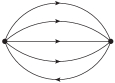
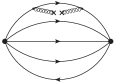
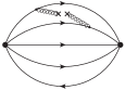
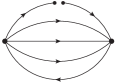
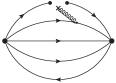
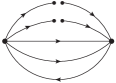
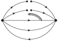
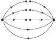
​​​​a    ​​​​b    ​​​​c ​​​​d    ​​​​e    ​​​​f ​​​​g    ​​​​h

Figure 1: Generic diagrams of the OPE terms for the correlators with the currents of the pentaquark states. Diagram (a) is the perturbative contribution at the leading order (LO). The figures (b)-(h) are diagrams for the nonperturbative contributions. We use here nonlocal condensate notation Mikhailov:1986be ; Mikhailov:1991pt ; Grozin:1985wj ; Grozin:1994hd ; Bakulev:2006wz ; Bakulev:2009ib for the graphical representation of the various contributions originating from the standard (local) condensates. Some of the nonperturbative diagrams contribute to few terms of the operator OPE, as it is specified in Tab. 1.

Term	LO	$\langle{\bar{q}q}\rangle$	$\langle{GG}\rangle$	$\langle{\bar{q}Gq}\rangle$	$\langle{\bar{q}q}\rangle^{2}$	$\langle{\bar{q}q}\rangle\langle{\bar{q}Gq}\rangle$	$\langle{\bar{q}q}\rangle^{3}$	$\langle{\bar{q}Gq}\rangle^{2}$
$D$	0	3	4	5	6	8	9	10
Diag.	a	d	b, c	d, e	f	f, g	h	f

Table 1: In the first row of the table, we list the vacuum condensates of the various operators that give a contribution to the OPE for the studied correlators. The second row provides the dimension of the operators. The dimension-7 condensate $\langle{GG}\rangle\langle{\bar{q}Gq}\rangle$ isn’t included in our study due to the smallness of the gluon-condensate terms. The third row denotes the correspondence of the operators to the diagrammatic representations in Fig. 1. Note that here we denote contributions from both light and s quarks condensates by $\langle{\bar{q}q}\rangle^{n}$ .

IV System of QCD SRs and Numerical Analysis

We construct the QCD SRs for the state with spin $s$ using the scalar functions $\Pi^{s}_{1}$ and $\Pi^{s}_{2}$ in the correlators Eq. (6). As discussed in the previous section, since the relativistic interpolating current can couple to the two states with opposite parities, the physical parameters, masses and the decay constants for the two states are coupled together in the QCD SRs. First, we present the system of the QCD SRs in the coupled forms and discuss how to decouple the system of the QCD SRs for each state of definite parity by using a proper combination of $\Pi^{s}_{1}$ and $\Pi^{s}_{2}$. In this section, we omit for simplicity the index $s$ in all formulas as far as the involved expressions are valid for any considered spin $s$.

In the framework of QCD SR Shifman:1978bx , the Borel transformation $\hat{B}$

$$\hat{B}_{Q^{2}\to M^{2}}\!\left[\Pi(Q^{2})\right]=\mathop{\text{lim}}\limits_{n\to\infty}\!\frac{(-Q^{2})^{n}}{\Gamma(n)}\!\left[\frac{d^{n}}{dQ^{2n}}\Pi(Q^{2})\right]_{Q^{2}=nM^{2}}\,,$$

is applied to both sides of Eq. (7). This transformation helps to reduce the SR uncertainties by suppressing the contributions from the excited resonances in the continuum and also higher-order OPE terms.

For the phenomenological part of the SR, we apply the phenomenological spectral densities, which are called by $\rho_{i}^{\text{ph}}(t)$ and appear on the right-hand side in Eq. (7). For all considered states, we assume that these spectral densities can be decomposed into contributions from the resonances of the considered states and the contribution from the continuum starting from the threshold $s_{0}$ appealing to the quark-hadron duality hypothesis

$$\rho_{1}^{\text{ph}}(t) = f^{2}_{+}\delta(t-m^{2}_{+})+f^{2}_{-}\delta(t-m^{2}_{-})$$

$$+\Theta(t-s_{0})\rho^{\text{OPE}}_{1}(t)\,,$$

$$\rho_{2}^{\text{ph}}(t) = f^{2}_{+}m_{+}\delta(t-m^{2}_{+})-f^{2}_{-}m_{-}\delta(t-m^{2}_{-})$$

$$+\Theta(t-s_{0})\rho^{\text{OPE}}_{2}(t)\,,$$

where the threshold $s_{0}$ is chosen to be the same for both parities and for both densities ($\rho_{1}^{\text{ph}}$ and $\rho_{2}^{\text{ph}}$). The OPE spectral densities $\rho^{\text{OPE}}_{i}(t)=\rho^{s}_{i}(t)$ are defined by Eq. (17). The decay constants $f_{\pm}$ and masses $m_{\pm}$ are given in Eqs. (10), (12), (15). Then, the resonance contributions to the phenomenological part of the SR are defined as follows

$${\cal R}^{\text{(res)}}_{1,k}(M^{2}) = f_{+}^{2}m_{+}^{2k}e^{-m_{+}^{2}/M^{2}}+f_{-}^{2}m_{-}^{2k}e^{-m_{-}^{2}/M^{2}}\,,$$

$${\cal R}^{\text{(res)}}_{2,k}(M^{2}) = f_{+}^{2}m_{+}^{2k+1}e^{-m_{+}^{2}/M^{2}}-f_{-}^{2}m_{-}^{2k+1}e^{-m_{-}^{2}/M^{2}}\,,$$

where we apply the Borel transformation to Eq. (7), as already discussed. Combining the full OPE results with the contribution from the continuum, we evaluate the theoretical part of the QCD SRs

$${\cal R}^{\text{(SR)}}_{i,k}(M^{2},s_{0})=\int_{s_{\text{th}}}^{s_{0}}\!dt\,\rho_{i}(t)\,t^{k}e^{-t/M^{2}}\,,$$

where the $k$-times derivatives with respect to $-1/M^{2}$ are taken after the Borel transformation. Finally, for each state of spin $s$=1/2, 3/2, 5/2, we obtain the following system of QCD SRs in the coupled form:

$${\cal R}^{\text{(res)}}_{1,k}(M^{2})={\cal R}^{\text{(SR)}}_{1,k}(M^{2},s_{0})\,,$$ (19)

$${\cal R}^{\text{(res)}}_{2,k}(M^{2})={\cal R}^{\text{(SR)}}_{2,k}(M^{2},s_{0})\,.$$

where $k\in Z_{+}\bigcup\{0\}$.

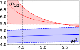
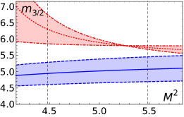
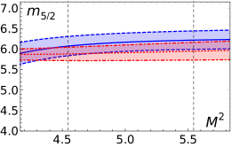
Figure 2: Borel parameter dependence of the mass $m_{s}(s_{0},M^{2})$ for a $uds$-$\bar{c}c$ flavor clustering, given by Eq. (23), referring to spin $s=1/2$ (left panel), spin $s=3/2$ (central panel), spin $s=5/2$ (right panel) for negative parity (blue solid line and blue band limited by dashed blue lines) and positive parity (red dotted line and red band limited by dot-dashed red lines). The central lines of the bands denote the dependence for the best fit threshold $s_{0}=\tilde{s}_{0}$. The bands show the dependence of the masses on the threshold $s_{0}$ varied in the threshold interval $s_{0}\in[s_{0}^{\text{min}},s_{0}^{\text{max}}]$. Vertical dotted black lines present the Borel windows $(M^{2}_{-},M^{2}_{+})$.

IV.1 Decoupled QCD SRs

This subsection is devoted to decoupling the SRs in Eqs. (19) into two QCD SR equations for each state of definite parity. It seems that there are four different ways to deal with this kind of coupled QCD SRs systems used in the pentaquark QCD SR studies. First, assuming that most of the contributions come from the lowest lying resonance of the considered parity, the contributions from the resonance of the opposite parity can be ignored and only the second equation in Eq. (19) has been considered. This approach has been applied to many studies on the states of $S=1/2$ and to pentaquark states Lee:2005ny ; Xiang:2017byz ; Chen:2016qju . In a second way, used in Azizi:2016dhy , one resolves the systems (19) by taking into account the states of both parities without decoupling the system. The third way is to get the decoupled QCD SRs by using the old-fashioned correlator Jido:1996ia ; Ohtani:2012ps . Here, we use a method that is similar to the fourth way Wang:2015epa , in which the system of SRs, see, Eq. (19), is decoupled into two QCD SRs for each state of definite parity.

To decouple the SRs given by Eqs. (19), we expand the region of validity for k to ${k\in\{n/2|n\in Z\}}$. This analytical continuation allows us to consider the following linear combination of Eqs. (19)

$${\cal R}^{\text{(SR)}}_{\pm,k}=\frac{1}{2}({\cal R}^{\text{(SR)}}_{1,k}\pm{\cal R}^{\text{(SR)}}_{2,k-1/2})\,,$$

$${\cal R}^{\text{(res)}}_{\pm,k}=\frac{1}{2}({\cal R}^{\text{(res)}}_{1,k}\pm{\cal R}^{\text{(res)}}_{2,k-1/2})\,.$$

As a result we can rewrite the SRs, given by Eq. (19), in decoupled form to read

$${\cal R}^{\text{(res)}}_{\pm,k}(M^{2}) = {\cal R}^{\text{(SR)}}_{\pm,k}(M^{2},s_{0})\,,$$ (20)

with

$${\cal R}^{\text{(res)}}_{\pm,k}(M^{2}) = f^{2}_{\pm}e^{-m^{2}_{\pm}/M^{2}}m^{2k}_{\pm}\,,$$

$${\cal R}^{\text{(SR)}}_{\pm,k}(M^{2},s_{0}) = \int_{s_{\text{th}}}^{s_{\pm}}dt\rho_{\pm}^{\text{OPE}}(t)t^{k}e^{-t/M^{2}}\,.$$

where the reparameterized spectral densities $\rho_{\pm}^{\text{OPE}}$ are related to $\rho_{1,2}^{\text{OPE}}$ (calculated by the OPE in Eq. (8)) as

$$\rho^{\text{OPE}}_{\pm}(t)=\frac{1}{2}\bigg{(}\rho^{\text{OPE}}_{1}(t)\pm\frac{\rho^{\text{OPE}}_{2}(t)}{\sqrt{t}}\bigg{)}\ .$$

The decoupled QCD SRs, Eq. (20), can be written in explicit form

$$f^{2}_{\pm}e^{-m^{2}_{\pm}/M^{2}}m^{2k}_{\pm}=\int_{s_{\text{th}}}^{s_{\pm}}dt\rho_{\pm}(t)t^{k}e^{-t/M^{2}}\,.$$ (21)

$$\begin{array}[]{|c|c||c|c|c|c|c|c|c|c|c|}\hline\cr\text{spin}&\text{flavor}&m_{-}(\tilde{s}_{0}),\text{GeV}&m_{+}(\tilde{s}_{0}),\text{GeV}&10^{3}f_{-}(\tilde{s}_{0}),\text{GeV}^{6}&10^{3}f_{+}(\tilde{s}_{0}),\text{GeV}^{6}&(s_{0}^{\text{min}},s_{0}^{\text{max}})&\tilde{s}_{0}&(M^{2}_{-},M^{2}_{+})&\delta(\tilde{s}_{0})\,,\%&r(\tilde{s}_{0})\\ \hline\cr\hline\cr 1/2&uds\text{-}\bar{c}c&4.4_{-0.3}^{+0.7}\pm 0.0&5.1_{-0.0}^{+1.0}\pm 0.1&1.8_{-0.7}^{+4.0}\pm 0.0&1.3_{-0.2}^{+3.9}\pm 0.0&(22.0,34.7)&25.1&(4.5,5.5)&3.8&0.05\\ \hline\cr 1/2&udc\text{-}\bar{c}s&4.5_{-0.2}^{+0.3}\pm 0.1&5.3_{-0.0}^{+0.3}\pm 0.2&2.0_{-0.5}^{+1.4}\pm 0.1&2.0_{-0.1}^{+1.4}\pm 0.0&(24.0,30.6)&26.1&(3.7,4.7)&5.0&0.13\\ \hline\cr 1/2&usc\text{-}\bar{c}d&4.6_{-0.2}^{+0.3}\pm 0.1&5.3_{-0.0}^{+0.3}\pm 0.2&2.1_{-0.6}^{+1.6}\pm 0.1&2.1_{-0.2}^{+1.6}\pm 0.1&(24.3,31.2)&26.5&(3.7,4.7)&5.1&0.14\\ \hline\cr 3/2&uds\text{-}\bar{c}c&4.9_{-0.2}^{+0.5}\pm 0.1&5.7_{-0.0}^{+0.6}\pm 0.2&1.9_{-0.6}^{+2.5}\pm 0.0&1.9_{-0.2}^{+2.6}\pm 0.0&(27.3,38.6)&30.2&(4.5,5.5)&4.7&0.13\\ \hline\cr 3/2&udc\text{-}\bar{c}s&4.8_{-0.1}^{+0.2}\pm 0.1&5.8_{-0.0}^{+0.2}\pm 0.3&1.9_{-0.4}^{+0.8}\pm 0.1&2.6_{-0.0}^{+0.8}\pm 0.1&(28.7,34.9)&30.8&(3.4,4.4)&7.4&0.32\\ \hline\cr 3/2&usc\text{-}\bar{c}d&4.9_{-0.1}^{+0.2}\pm 0.1&5.8_{-0.0}^{+0.2}\pm 0.3&2.1_{-0.4}^{+0.8}\pm 0.1&3.0_{-0.0}^{+0.9}\pm 0.1&(29.5,36.1)&31.8&(3.4,4.4)&8.2&0.36\\ \hline\cr 5/2&uds\text{-}\bar{c}c&6.2_{-0.3}^{+0.1}\pm 0.1&6.0_{-0.3}^{+0.1}\pm 0.0&12.1_{-6.4}^{+3.8}\pm 0.1&15.6_{-6.1}^{+3.3}\pm 0.1&(39.2,50.0)&46.3&(4.5,5.5)&1.2&0.51\\ \hline\cr 5/2&udc\text{-}\bar{c}s&6.0_{-0.4}^{+0.1}\pm 0.1&5.9_{-0.3}^{+0.1}\pm 0.0&7.2_{-4.1}^{+2.5}\pm 0.1&12.2_{-4.9}^{+2.6}\pm 0.1&(37.6,50.0)&45.5&(3.7,4.7)&1.7&0.64\\ \hline\cr 5/2&usc\text{-}\bar{c}d&6.3_{-0.3}^{+0.0}\pm 0.1&6.0_{-0.3}^{+0.0}\pm 0.1&9.9_{-5.3}^{+0.0}\pm 0.1&15.1_{-5.9}^{+0.0}\pm 0.2&(40.6,50.0)&50.0&(3.8,4.8)&2.1&0.75\\ \hline\cr\end{array}$$

Table 2: QCD SR results for masses $m_{\pm}$ and decay constants $f_{\pm}$ given for a pentaquark with both parities with spin 1/2, 3/2, 5/2 (first column) for three cases of flavor-clustering (second column). For all cases considered in this table, we apply the type-1 currents defined in Eqs. (9), (11), (14). Central values of masses (2nd and 3rd columns) and decay constants (4th and 5th columns) given at the best-fit threshold $(\tilde{s}_{0})$ (see column 8th). The first error bars from the third to the sixth column represent the variation with respect to the threshold value in the interval $(s_{0}^{\text{min}},s_{0}^{\text{max}})$ given in the 7th column. The second error bars in the columns from the third to the sixth represent the variation in the Borel window $(M^{2}_{-},M^{2}_{+})$ (see 9th column). The criteria values $\delta(\tilde{s}_{0})$ are given for each state in percentages in the 10th column. Additionally, the last column represents the criteria of the resonance contribution $r_{1}(\tilde{s}_{0})$.

IV.2 Numerical Analysis

In this subsection, we extract the masses and the decay constants from the constructed QCD SRs. The first step is to define the Borel window $M^{2}\in[M^{2}_{-},M^{2}_{+}]$ by the conditions

$$\frac{{\cal R}^{\text{(SR)}}_{2,9,0}(M^{2}_{-},\infty)}{{\cal R}^{\text{(SR)}}_{2,0}(M^{2}_{-},\infty)}<\frac{1}{10}\,,~{}~{}M^{2}_{+}=M^{2}_{-}+\Delta M^{2}\,.$$

The low boundary $M^{2}_{-}$ of the Borel window insures that the dimension-9 condensate $\langle{\bar{q}q}\rangle^{3}$ contributes less than 10% to the total value of the correlator. Here we use the following notation for the OPE contribution of dimension D

$${\cal R}^{\text{(SR)}}_{i,D,k}(M^{2},s_{0})=\int_{s_{\text{th}}}^{s_{0}}\!dt\,\rho_{iD}(t)\,t^{k}e^{-t/M^{2}}\,.$$

The upper boundary $M^{2}_{+}$ is determined by the above condition by setting $\Delta M^{2}=1$ GeV². We don’t follow the common practice to define the upper boundary $M^{2}_{+}$ by the condition that the resonance contribution gives at least 10% to the total value of the correlator, $r_{i}(s_{0})>1/10$, for $i=1\,,2$, where

$$r_{i}(s_{0})=\frac{{\cal R}^{\text{(SR)}}_{i,0}(M^{2}_{+},s_{0})}{{\cal R}^{\text{(SR)}}_{i,0}(M^{2}_{+},\infty)}\,.$$

The values of this ratio are given in Tables 2, 3, and 4 for the considered SRs. Note that most of the SRs yield values of this ratio above 1/10. Having an equal size of the Borel window $\Delta M^{2}$ for all SRs allows us to compare the SR stability criteria for different SRs without violating the condition $r_{i}(s_{0})>1/10$. To control this condition we introduce the collective value

$$r(s_{0})=\textbf{min}(r_{1}(s_{0}),r_{2}(s_{0}))\,,$$

that can be found in the last column of Tables 2, 3, and 4.

$$\begin{array}[]{|c|c||c|c|c|c|c|c|c|c|c|}\hline\cr\text{spin}&\text{type}&m_{-}(\tilde{s}_{0}),\text{GeV}&m_{+}(\tilde{s}_{0}),\text{GeV}&10^{3}f_{-}(\tilde{s}_{0}),\text{GeV}^{6}&10^{3}f_{+}(\tilde{s}_{0}),\text{GeV}^{6}&(s_{0}^{\text{min}},s_{0}^{\text{max}})&\tilde{s}_{0}&(M^{2}_{-},M^{2}_{+})&\delta(\tilde{s}_{0})\,,\%&r(\tilde{s}_{0})\\ \hline\cr\hline\cr 1/2&1(1)&4.4_{-0.3}^{+0.7}\pm 0.0&5.1_{-0.0}^{+1.0}\pm 0.1&1.8_{-0.7}^{+4.0}\pm 0.0&1.3_{-0.2}^{+3.9}\pm 0.0&(22.0,34.7)&25.1&(4.5,5.5)&3.8&0.05\\ \hline\cr 1/2&2(1)&4.4_{-0.3}^{+0.9}\pm 0.0&5.1_{-0.0}^{+1.0}\pm 0.1&1.8_{-0.7}^{+5.6}\pm 0.0&1.3_{-0.2}^{+5.4}\pm 0.0&(22.0,36.6)&25.1&(4.6,5.6)&4.2&0.04\\ \hline\cr 1/2&3(0)&5.9_{-0.0}^{+0.9}\pm 0.2&5.1_{-0.2}^{+0.6}\pm 0.0&1.4_{-0.1}^{+2.8}\pm 0.0&1.6_{-0.5}^{+2.7}\pm 0.0&(29.6,43.1)&32.7&(4.9,5.9)&4.0&0.1\\ \hline\cr 1/2&4(0)&5.9_{-0.0}^{+0.9}\pm 0.2&5.1_{-0.2}^{+0.6}\pm 0.0&4.2_{-0.3}^{+8.3}\pm 0.1&4.7_{-1.5}^{+8.1}\pm 0.1&(29.6,43.1)&32.7&(4.9,5.9)&4.0&0.1\\ \hline\cr 3/2&1(1)&4.9_{-0.2}^{+0.5}\pm 0.1&5.7_{-0.0}^{+0.6}\pm 0.2&1.9_{-0.6}^{+2.5}\pm 0.0&1.9_{-0.2}^{+2.6}\pm 0.0&(27.3,38.6)&30.2&(4.5,5.5)&4.7&0.13\\ \hline\cr 3/2&2(0)&6.2_{-0.4}^{+0.1}\pm 0.0&6.6_{-0.1}^{+0.2}\pm 0.0&6.0_{-3.1}^{+0.9}\pm 0.0&4.9_{-2.7}^{+1.0}\pm 0.0&(38.8,50.0)&47.8&(4.9,5.9)&0.8&0.4\\ \hline\cr\end{array}$$

Table 3: QCD SR results for the masses $m_{\pm}$ and the decay constants $f_{\pm}$ given for a pentaquark of both parities with spin 1/2, 3/2 (first column) and for a $udc$-$\bar{c}s$ flavor-clustering. The second column denotes the type of the current and the spin of the $\bar{c}s$-part given in the parentheses. The types of the currents are defined in Eqs. (9) and (11). See the caption of Table 2 for more details.

$$\begin{array}[]{|c|c||c|c|c|c|c|c|c|c|c|}\hline\cr\text{spin}&\text{type}&m_{-}(\tilde{s}_{0}),\text{GeV}&m_{+}(\tilde{s}_{0}),\text{GeV}&10^{3}f_{-}(\tilde{s}_{0}),\text{GeV}^{6}&10^{3}f_{+}(\tilde{s}_{0}),\text{GeV}^{6}&(s_{0}^{\text{min}},s_{0}^{\text{max}})&\tilde{s}_{0}&(M^{2}_{-},M^{2}_{+})&\delta(\tilde{s}_{0})\,,\%&r(\tilde{s}_{0})\\ \hline\cr\hline\cr 1/2&1&4.4_{-0.2}^{+0.4}\pm 0.0&5.1_{-0.0}^{+0.4}\pm 0.1&1.6_{-0.5}^{+1.5}\pm 0.0&1.4_{-0.2}^{+1.5}\pm 0.0&(22.6,29.9)&24.7&(3.8,4.8)&4.1&0.1\\ \hline\cr 3/2&1&4.8_{-0.1}^{+0.2}\pm 0.1&5.7_{-0.0}^{+0.3}\pm 0.3&1.8_{-0.4}^{+0.8}\pm 0.1&2.2_{-0.0}^{+0.8}\pm 0.1&(28.2,34.7)&30.4&(3.4,4.4)&6.7&0.3\\ \hline\cr 5/2&1&6.0_{-0.4}^{+0.2}\pm 0.1&5.9_{-0.3}^{+0.1}\pm 0.0&6.9_{-3.9}^{+2.6}\pm 0.1&11.6_{-4.7}^{+2.7}\pm 0.1&(37.6,50.0)&45.3&(3.8,4.8)&1.7&0.6\\ \hline\cr\end{array}$$

Table 4: QCD SR results for the masses $m_{\pm}$ and the decay constants $f_{\pm}$ given for a $(udc)$-$(\bar{c}u)$ pentaquark of both parities with spin 1/2, 3/2, 5/2 (first column) with type 1 current for each case (second column). See the caption of Tab. 2 for more details.

The values of the masses and the decay constants can be extracted from the decoupled QCD SRs, Eq. (21), through averaging in the Borel window $M^{2}\in[M^{2}_{-},M^{2}_{+}]$

$$m_{\pm}(s_{0}) = \frac{1}{n+1}\sum\limits_{j=0}^{n}m_{\pm}(s_{0},M^{2}_{j})\,,$$ (22)

$$f^{2}_{\pm}(s_{0}) = \frac{1}{n+1}\sum\limits_{j=0}^{n}e^{m_{\pm}^{2}/M^{2}_{j}}{\cal R}^{\text{(SR)}}_{\pm,0}(M^{2}_{j},s_{0})\,,$$

where $n=8$, $M^{2}_{j}=M^{2}_{-}+(M^{2}_{+}-M^{2}_{-})j/n$ and

$$m^{2\Delta k}_{\pm}(s_{0},M^{2}) = \frac{{\cal R}^{\text{(SR)}}_{\pm,k+\Delta k}(M^{2},s_{0})}{{\cal R}^{\text{(SR)}}_{\pm,k}(M^{2},s_{0})}\,.$$ (23)

We present our result for the case $(k,\Delta k)=(1/2,1/2)$. We have also checked two extra choices: $(0,1/2)$ and $(1/2,1)$ for $(k,\Delta k)$ to confirm the small dependence of our results on $k$ and $\Delta k$. Similar decoupled QCD SRs have been considered in Wang:2015epa with $(k,\Delta k)=(1/2,1)$. Borel parameter dependencies of the masses $m_{\pm}(s_{0},M^{2})$ for the $uds-{\bar{c}}c$ case are shown in Fig. 2 for the best-fit threshold value $s_{0}=\tilde{s}_{0}$. Additionally, the bands around the central value show the dependence of the masses on the threshold $s_{0}$ varied in the interval $s_{0}\in[s_{0}^{\text{min}},s_{0}^{\text{max}}]$.

To find the best values of the five parameters $f_{\pm}$, $m_{\pm}$, $s_{0}$, we demand the minimization of the Borel parameter dependence of the original coupled SRs, Eqs. (19) i.e.,

$$\delta_{i}^{k}(s_{0})=\!\!\!\!\mathop{\textbf{max}}\limits_{M^{2}\in[M^{2}_{-},M^{2}_{+}]}\frac{{\cal R}^{\text{(res)}}_{i,k}(M^{2})-{\cal R}^{\text{(SR)}}_{i,k}(M^{2},s_{0})}{{\cal R}^{\text{(res)}}_{i,k}(M^{2})}\cdot 100\%$$

with masses and decay constants in ${\cal R}^{\text{(res)}}$ fixed by Eqs. (22). The minimization of the Borel parameter dependence of the original coupled SRs instead of the decoupled SRs helps avoiding possible uncertainties related to the analytical continuation of the SRs. Finally, we combine the four criteria in one to get

$$\delta(s_{0})=\textbf{max}(\delta_{1}^{k}(s_{0}),\delta_{1}^{k+\Delta k}(s_{0}),\delta_{2}^{k-\frac{1}{2}}(s_{0}),\delta_{2}^{k+\Delta k-\frac{1}{2}}(s_{0}))\,.$$

We use this combined criterion to define the best-fit value for the threshold $\tilde{s_{0}}$ and the threshold interval $s_{0}\in[s_{0}^{\text{min}},s_{0}^{\text{max}}]$, where subject to the condition

$$\delta(s_{0})<\delta(\tilde{s}_{0})+1\,.$$

The values of the threshold $\tilde{s}_{0}$ and the interval boundaries $s_{0}^{\text{min}}$ and $s_{0}^{\text{max}}$ can be found in Tables 2, 3, 4 for all considered states. From these values we obtain the masses $m_{\pm}(\tilde{s}_{0})$ and the decay constant $f_{\pm}(\tilde{s}_{0})$ at $\tilde{s}_{0}$ given in Table 2 together with their variations in the threshold interval and the variations in the Borel window.

The central value $\bar{m}$ of the mass and the uncertainty $\Delta_{s}m$ related to the threshold are defined by

$$\bar{m}_{\pm} = \frac{1}{2}\left(\mathop{\textbf{max}}\limits_{s_{0}}~{}m_{\pm}(s_{0})+\mathop{\textbf{min}}\limits_{s_{0}}~{}m_{\pm}(s_{0})\right)$$

$$\Delta_{s}m_{\pm} = \frac{1}{2}\left(\mathop{\textbf{max}}\limits_{s_{0}}~{}m_{\pm}(s_{0})-\mathop{\textbf{min}}\limits_{s_{0}}~{}m_{\pm}(s_{0})\right)\,,$$

where max (min) gives the maximum (minimum) value of the function $m_{\pm}(s_{0})$ in the threshold interval $s_{0}\in[s_{0}^{\text{min}},s_{0}^{\text{max}}]$. The error bars related to the Borel parameter variation in the Borel window interval $M^{2}\in[M^{2}_{-},M^{2}_{+}]$ is calculated by

$$\Delta_{M}m_{\pm} = \frac{1}{2}\left(\mathop{\textbf{max}}\limits_{M^{2}}~{}m_{\pm}(\tilde{s}_{0},M^{2})-\mathop{\textbf{max}}\limits_{M^{2}}~{}m_{\pm}(\tilde{s}_{0},M^{2})\right)\,.$$

Final results for the mass are given in Fig. 3 and Tab. 5 by the central value mass $\bar{m}$ and the total uncertainty $\Delta m$

$$m_{\pm}=\bar{m}_{\pm}+\Delta m_{\pm}\,,$$ (24)

where the total uncertainty is the sum of the above uncertainties

$$\Delta m_{\pm} = \Delta_{s}m_{\pm}+\Delta_{M}m_{\pm}$$ (25)

that includes only uncertainties stemming from the SR analysis and don’t include the uncertainties of the condensates.

The following numerical values of the vacuum condensates and masses have been used for the numerical analysis

$$\langle{(\alpha_{S}/\pi)G^{2}}\rangle=0.012~{}\text{GeV}^{3}\,,~{}~{}\langle{\bar{q}q}\rangle=(-0.25)^{3}~{}\text{GeV}^{3}\,,~{}~{}$$

$$\langle{\bar{q}Gq}\rangle=\langle{\bar{q}G_{\mu\nu}\sigma_{\mu\nu}q}\rangle=m_{0}^{2}\langle{\bar{q}q}\rangle,~{}m_{0}^{2}=0.8~{}\text{GeV}^{2}\,,~{}~{}$$

$$m_{q}=0\,,~{}~{}m_{s}=0.1~{}\text{GeV}\,,~{}~{}m_{c}=1.23~{}\text{GeV}\,,~{}~{}~{}~{}$$

$$\langle{\bar{s}s}\rangle=f_{s}\langle{\bar{q}q}\rangle\,,~{}~{}\langle{\bar{s}Gs}\rangle=f_{s}\langle{\bar{q}Gq}\rangle\,,~{}~{}f_{s}=0.8\,.$$

The lowest threshold value is taken to be $s_{\text{th}}=6.5$ GeV², see Eq. (7).

The QCD SR technique described above has been applied using various pentaquark currents. First, we studied the type-1 current for the three flavor configuration ($uds$-$\bar{c}c$, $udc$-$\bar{c}s$, $usc$-$\bar{c}d$), see the results in Table 2. Second, in Table 3, we obtained results for some alternative currents to estimate their relevance. Finally, we used our method to study the $udc$-$\bar{c}u$ flavor configuration, in order to see whether $P_{c}^{+}(4312)$, $P_{c}^{+}(4440)$, and $P_{c}^{+}(4457)$, observed by the LHCb Collaboration, can be understood as a pentaquark of two clusters in a color-octet state. The detailed results given in Table 4 will be discussed in the next section.

V Discussion and Summary

In this section, we discuss the results obtained in the previous sections on the basis of the constructed QCD SRs for pentaquark states. We have constructed the currents for $udsc\bar{c}$ pentaquarks of spin-1/2, 3/2, 5/2 that have two clusters of a color-octet. The first cluster consists of three quarks $q^{1}q^{2}q^{3}$ which has the same flavor structure as the flavor singlet state of $uds$, while the second cluster consists of quark-antiquark $\bar{c}q^{4}$. There are four options for flavor clustering $q^{1}q^{2}q^{3}$-$\bar{c}q^{4}$ ($uds$-$\bar{c}c$, $udc$-$\bar{c}s$, $usc$-$\bar{c}d$, $dsc$-$\bar{c}u$). The results for $dsc$-$\bar{c}u$ and $usc$-$\bar{c}d$ are identical in our approach and, therefore, we present here only results for the $dsc$-$\bar{c}u$ configuration. The main predictions for pentaquarks are presented for the type-1 current, that has a spin-1 $\bar{c}q^{4}$ part. In section III, in addition to these main currents, we have also introduced the alternative currents for spin-1/2 states and spin-3/2 states, see Eq. (9) and Eq. (11). Particularly, we are interested in the alternative currents with a spin-0 quark-antiquark cluster: type-3 and type-4 for a spin-1/2 current and type-2 for a spin-3/2 current. In Table 3, we presented the results for these alternative currents of a $udc$-$\bar{c}s$ configuration with a spin-0 $\bar{c}s$-cluster in comparison with the main currents that have a spin-1 $\bar{c}s$-cluster. One can see that these types of currents lead to larger masses compared to those for the spin-1 cases for both spin-1/2 and spin-3/2 pentaquarks. We have also checked that a similar conclusion is valid for other flavor configurations. This observation agrees with Irie:2017qai , where it has been shown that the two-quark cluster with spin 1 in $uds$-${\bar{c}}c$ system yield the most stable result. In Table 3, we have also considered the alternative current for a spin 1/2 state containing a spin-1 $\bar{c}s$-cluster (type-2 for spin-1/2 current) and found that this current gives the same result. Therefore, the main results in our paper are given for the hidden pentaquark states with a spin-1 quark-antiquark cluster.

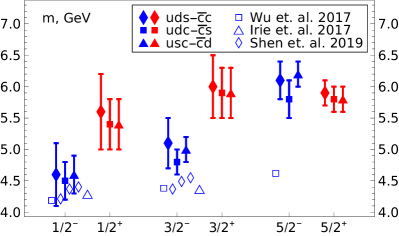
Figure 3: QCD SRs results for masses of pentaquarks with spins 1/2, 3/2, 5/2 for the even parity (red color errorbars) and for the odd parity (blue color errorbars) are given for three types of flavor clustering: $uds$-$\bar{c}c$ (diamonds), $udc$-$\bar{c}s$ (squares), $usc$-$\bar{c}d$ (triangles). Central value and width of errorbars are given in Eq. (24) and Eq. (25). The result of our calculations are depicted by $\blacklozenge$ for $uds$-$\bar{c}c$, by $\blacksquare$ for $udc$-$\bar{c}s$, by $\blacktriangle$ for $usc$-$\bar{c}d$. The results of other theoretical predictions for $udsc\bar{c}$ pentaquark are denoted by $\square$ for the color-magnetic interaction based study Wu:2017weo , $\lozenge$ for the framework of the coupled channel unitary approach with the local hidden gauge formalism Wu:2010jy ; Wu:2010vk ; Shen:2019evi , $\triangle$ for the quark model result Irie:2017qai .

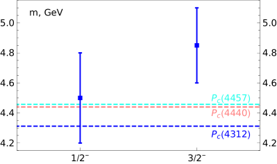
Figure 4: The masses of a recently observed by LHCb Aaij:2019vzc states are shown by the dashed lines in comparison to our QCD SR estimations (blue errorbars) for the lightest states with a color-octet substructure. For more details see Tab. 4.

Using type-1 currents, we have considered three types of flavor clustering ($uds$-$\bar{c}c$, $udc$-$\bar{c}s$, $usc$-$\bar{c}d$) and found that they have similar masses and decay constants, see Table 2. Therefore, we expect that these configurations have equal chances to be observed. The consideration of a possible mixing between these configurations is outside the scope of this work. Another observation is that the larger spin states give larger masses.

$$\begin{array}[]{|c||c|c||c|c||c|c|}\hline\cr\text{flavor}&1/2^{-}&1/2^{+}&3/2^{-}&3/2^{+}&5/2^{-}&5/2^{+}\\ \hline\cr\hline\cr uds\text{-}\bar{c}c&4.6(5)&5.6(6)&5.1(4)&6.0(5)&6.1(3)&5.9(2)\\ \hline\cr udc\text{-}\bar{c}s&4.5(3)&5.4(4)&4.8(2)&5.9(4)&5.8(3)&5.8(2)\\ \hline\cr usc\text{-}\bar{c}d&4.6(3)&5.4(4)&5.0(2)&5.9(4)&6.2(2)&5.8(2)\\ \hline\cr\end{array}$$

Table 5: Final QCD SR results for $udsc\bar{c}$ pentaquark masses for both parities with spin 1/2, 3/2, 5/2. Values are given according Eq. (24). For more details see Table 2.

Our results are presented in comparison with other theoretical predictions Shen:2019evi ; Wu:2017weo ; Irie:2017qai for $uds\bar{c}c$ pentaquark in Fig. 3. The masses from the effective Lagrangian framework Shen:2019evi for the $uds$-$\bar{c}c$ flavor configuration with a color-singlet substructures, depicted by $\lozenge$, are lower for the spin 3/2 case and comparable consistently well with our predictions for the spin 1/2 case referring to a pentaquark state with a color-octet substructure. The quark model prediction for $uds$-${\bar{c}}c$ Irie:2017qai , noted by $\triangle$ in Fig. 3, is in very good agreement with our result for a spin-1/2 pentaquark, while the prediction for spin-3/2 case is different. Note that apart of result Irie:2017qai , we compare our predictions with the results for the configurations that are different from the configurations considered in our work. Therefore, the comparisons are given only for the reference.

In order to see whether any of the pentaquarks observed by the LHCb Collaboration could be understood as a pentaquark composed of two clusters in the color-octet state, we study the pentaquark with the assumption that it is formed by the two clusters $udc$-$\bar{c}u$, where the three-quark cluster has a flavor-singlet structure. Therefore, we don’t have alternative to $udc$-$\bar{c}u$ flavor clustering as opposite to the $uds\bar{c}c$ pentaquark. QCD SR results for the masses $m_{\pm}$ and decay constants $f_{\pm}$ for such a pentaquark are presented in Table 4 for spin 1/2, 3/2, 5/2 and both parities. To make a point, we present the lightest state masses from this table in Fig. 4 together with the states recently observed by the LHCb Collaboration. As shown in this figure, the obtained mass for a spin-1/2 $udc$-$\bar{c}u$ pentaquark, is in agreement with the experimental value. Since the flavor content and the mass of the pentaquarks observed by LHCb are known only, we conclude that if the observed state has spin 1/2 and negative parity, it could be described as a state with two color-octet clusters.

It had been shown Kondo:2004cr ; Lucha:2019pmp that the correlator for a pentaquark state could include the two-hadron-reducible contributions, which are given by convolution of baryon and meson correlators that is not related to pentaquark. This problem of QCD SRs has been addressed in the series of work Lucha:2019pmp ; Lucha:2019cpe ; Lucha:2019cdc for tetraquark QCD SRs, where authors expect that similar problem could affects also SR for pentaquarks. As it has been shown for pentaquark considered in Lee:2004xk ; Agaev:2019qqn , the direct subtraction of a problematic two-hadron contributions from the correlator leads to incorrect results. To avoid this problem, the authors of Lee:2004xk utilized soft-kaon theorem and demonstrated that these type of problematic terms contribute less than 10% of the sum rules. We propose that the type of pentaquark currents constructed in this work is a solution for this problem of pentaquark SRs, due to the fact that such currents can not be factorized to the product of meson and baryon currents, see the relevant discussion in Appendix C.

To summarize, we have estimated the masses of the various hidden-charm pentaquarks with color-octet substructure and with $J^{PC}=$1/2^±, 3/2^±, 5/2^± in the framework of QCD SRs. We have constructed the currents for a particular configuration of pentaquark states, which consists of a three-quark cluster with the same flavor structure as the flavor singlet combination $uds$, and, additionally, of a quark-antiquark cluster, where both clusters are in a color-octet state. In our work, three possible types of flavor-clustering of the currents has been considered. To obtain QCD sum rules, the operator product expansion for the correlators with the constructed interpolating currents has been performed up to the level of dimension-10 condensates. From the constructed QCD SRs the masses and decay constants of the pentaquark states have been extracted. Numerical values are given in detail in Table 2, and are briefly summarized in Table 5.

VI Acknowledgment

We would like to thank N. Stefanis, M. Elbistan, D. Melikhov, Ju-Jun Xie and Hua-Xing Chen for stimulating discussions and useful remarks. We were inspired to perform this study by Nikolai Kochelev, who passed suddenly away in 2018. This work was supported by the National Natural Science Foundation of China (Grant No. 11975320), the National Key Research and Development Program of China (No. 2016YFE0130800), the Chinese Academy of Sciences President’s International Fellowship Initiative (PIFI Grant No. 2019PM0036). The work of H.-J. Lee was supported by the Basic Science Research Program through the National Research Foundation of Korea (NRF) funded by the Ministry of Education under Grant No. 2016R1D1A1A09920078. The work has been partially supported by the Ministry of Education and Science of the Russian Federation: Projects No. 3.6371.2017/8.9 and No. 3.6439.2017/8.9.

Appendix A Projectors for 3/2-spin correlator

We follow the common practice to extract the $g_{\mu\nu}$-term of the $3/2$ correlator and consider only the largest spin contribution. Here, we formalize this extraction by introducing the appropriate projectors. The general form of the tensor can be written in the following way

$$P_{\mu\nu}(q^{2}) = \sum\limits_{i=1}^{5}(c_{1i}\hat{q}+c_{2i})t^{i}_{\mu\nu}=\sum\limits_{j=1}^{10}C_{j}\tilde{t}^{j}_{\mu\nu}\,,$$ (26)

where we consider only P-even terms. The relation between two forms is given by $\tilde{t}^{2i}=t^{i}$, $\tilde{t}^{2i-1}=\hat{q}t^{i}$, $C_{2i}=c_{2i}$, $C_{2i-1}=c_{1i}$ with $i=1,\cdots\,5$. The linearly independent set $t^{j}_{\mu\nu}$ of all possible structures is defined as follows

$$t^{j}_{\mu\nu}=\left(-g_{\mu\nu},\gamma_{\mu}\gamma_{\nu},\frac{q_{\mu}q_{\nu}}{q^{2}},q_{\mu}\gamma_{\nu}-q_{\nu}\gamma_{\mu},q_{\mu}\gamma_{\nu}+q_{\nu}\gamma_{\mu}\right)_{j}\,.$$

A linear combination of tensors $\tilde{t}_{\mu\nu}$ can be used to construct the projectors as

$$P^{3/2,k}_{\mu\nu}=M^{-1}_{kl}\tilde{t}^{l}_{\mu\nu}\,,$$

where the matrix $M_{kl}$ reads

$$M_{kl}=Tr\left(\tilde{t}^{l}_{\mu\nu}\tilde{t}^{k}_{\mu\nu}\right)\,.$$

Then we can extract the coefficients $C_{j}$ from the expansion expressed by Eq. 26

$$C_{k}=Tr\left(P_{\mu\nu}(q^{2})P^{3/2,k}_{\mu\nu}\right).$$

The inverse of the matrix $M$ is given by

$$24s^{2}M^{-1}=$$

$$\small\left(\begin{array}[]{cccccccccc}s&0&-s&0&2s&0&0&s&0&0\\ 0&s^{2}&0&-s^{2}&0&2s^{2}&s&0&0&0\\ -s&0&-s&0&0&0&0&s&0&0\\ 0&-s^{2}&0&-s^{2}&0&0&s&0&0&0\\ 2s&0&0&0&12s&0&0&0&0&-2s\\ 0&2s^{2}&0&0&0&4s^{2}&0&0&2s&0\\ 0&s&0&s&0&0&-2&0&0&0\\ s&0&s&0&0&0&0&0&0&0\\ 0&0&0&0&0&2s&0&0&-1&0\\ 0&0&0&0&-2s&0&0&0&0&s\\ \end{array}\right)\,,$$ (37)

where $s=q^{2}$. Using the projectors $P^{3/2,1}_{\mu\nu}$ and $P^{3/2,2}_{\mu\nu}$, the densities, Eq. (13), can recast in the form

$$\rho^{3/2}_{1}(s) = \frac{-1}{24\pi s}{\rm Tr}\bigg{[}\textbf{Im}\Pi^{3/2}_{\mu\nu}(s)\hat{q}\bigg{(}g^{\mu\nu}+\gamma^{\mu}\gamma^{\nu}-\frac{2q^{\mu}q^{\nu}}{q^{2}}\bigg{)}\bigg{]}$$

$$+\frac{1}{24\pi s}{\rm Tr}\bigg{(}\textbf{Im}\Pi^{3/2}_{\mu\nu}(s)(q^{\mu}\gamma^{\nu}-q^{\nu}\gamma^{\mu})\bigg{)}\,,$$

$$\rho^{3/2}_{2}(s) = \frac{-1}{24\pi}{\rm Tr}\bigg{[}\textbf{Im}\Pi^{3/2}_{\mu\nu}(s)\bigg{(}g^{\mu\nu}+\gamma^{\mu}\gamma^{\nu}-\frac{2q^{\mu}q^{\nu}}{q^{2}}\bigg{)}\bigg{]}$$ (38)

$$-\frac{1}{24\pi s}{\rm Tr}\bigg{(}\textbf{Im}\Pi^{3/2}_{\mu\nu}(s)\hat{q}(q^{\mu}\gamma^{\nu}-q^{\nu}\gamma^{\mu})\bigg{)}\,.$$

Appendix B Projectors for 5/2-spin correlator

To extract the terms of the largest spin state from the correlator, the projector method is applied. Similarly to Eq. (26), the general form of the correlator can be written as follows

$$P_{\mu\nu,\alpha\beta}(q^{2}) = \sum\limits_{i=1}^{14}(c_{1i}\hat{q}+c_{2i})t^{i}_{\mu\nu,\alpha\beta}=\sum\limits_{j=1}^{28}C_{j}\tilde{t}^{j}\,,$$ (39)

where the relation between the two forms is given by $\tilde{t}^{2i}=t^{i}_{\mu\nu,\alpha\beta}$, $\tilde{t}^{2i-1}=\hat{q}t^{i}_{\mu\nu,\alpha\beta}$, $C_{2i}=c_{2i}$, $C_{2i-1}=c_{1i}$ with $i=1,\cdots\,14$. We consider only P-even terms which are symmetric with respect to $\mu\nu$ and $\alpha\beta$. The linearly independent set $t^{i}_{\mu\nu,\alpha\beta}$ of all possible structures is defined as

$$\!\!\!\!\!\!t^{i}_{\mu\nu,\alpha\beta}=\hat{S}_{\mu\nu}\hat{S}_{\alpha\beta}\left(\right.\frac{g_{\mu\alpha}g_{\nu\beta}}{4},\frac{g_{\mu\nu}g_{\alpha\beta}}{4},\frac{g_{\mu\alpha}\gamma_{\nu}\gamma_{\beta}}{4},g_{\mu\alpha}\frac{q_{\nu}q_{\beta}}{q^{2}},$$

$$\!\!g_{\mu\nu}\frac{q_{\alpha}q_{\beta}}{4q^{2}},g_{\alpha\beta}\frac{q_{\mu}q_{\nu}}{4q^{2}},g_{\mu\nu}\frac{\gamma_{\alpha}q_{\beta}}{2},g_{\alpha\beta}\frac{\gamma_{\mu}q_{\nu}}{2},g_{\mu\alpha}q_{\nu}\gamma_{\beta},$$

$$\!\!\left.g_{\mu\alpha}q_{\beta}\gamma_{\nu},\frac{q_{\mu}q_{\nu}}{2q^{2}}\gamma_{\alpha}q_{\beta},\frac{q_{\alpha}q_{\beta}}{2q^{2}}\gamma_{\mu}q_{\nu},\frac{q_{\mu}q_{\alpha}}{q^{2}}\gamma_{\nu}\gamma_{\beta},\frac{q_{\mu}q_{\nu}q_{\alpha}q_{\beta}}{q^{4}}\right)_{i}\,,$$

where the operator $\hat{S}_{\mu\nu}$ symmetrizes the tensor as ${\hat{S}_{\mu\nu}t_{\mu\nu}=t_{\mu\nu}+t_{\nu\mu}}$. Linear combination of these tensors can be used as the projectors

$$P^{5/2,k}_{\mu\nu,\alpha\beta}=M^{-1}_{kl}\tilde{t}^{l}$$ (40)

to extract the coefficients $C_{j}$ of the expansion, Eq. (39) notably,

$$C_{j}=Tr\left(P_{\mu\nu,\alpha\beta}P^{5/2,j}_{\mu\nu\alpha\beta}\right)$$

with the matrix

$$M_{kl}=Tr\left(\tilde{t}^{l}_{\mu\nu,\alpha\beta}\tilde{t}^{k}_{\mu\nu,\alpha\beta}\right)\,.$$

We provide only the first two rows of the inverse matrix, which define the projectors $P^{5/2,1}$ and $P^{5/2,2}$ applied to extract the spin-5/2 spectral densities, Eq. (16):

$$M^{-1}_{1l}120q^{2} = (2,0,-2,0,1,0,-2,0,2,0,2,0,0,0,0,0,0,$$

$$-1,0,1,0,2,0,-2,-1,0,4,0)_{l}\,,$$

$$M^{-1}_{2l}120q^{2} = (0,2q^{2},0,-2q^{2},0,q^{2},0,-2q^{2},0,2q^{2},0,2q^{2},$$

$$\!\!\!\!\!\!\!\!0,0,0,0,-1,0,1,0,2,0,-2,0,0,-q^{2},0,4q^{2})_{l}\,.$$

Other rows of the inverse matrix are not used in our work but could be obtained from the above equations.

Appendix C Currents in color subspace

Here, we consider the relation of the pentaquarks with different configurations: diquark-diquark-antiquark clustering $J_{\bar{3}}\sim qq$-$qq$-$\bar{q}$ with an anti-triplet color substructure suggested in Jaffe:2003sg ; Sugiyama:2003zk ; Lee:2005ny , a molecule form $J_{1}\sim qqq$-$\bar{q}q$ with color-singlet parts, see Guo:2017jvc , and the combination $J_{8}\sim qqq$-$\bar{q}q$ with color-octet compounds studied here. First, we consider only the color part of these currents

$$J_{8}^{\text{c}} \equiv (\epsilon_{a_{1}a_{2}a_{0}}t^{m}_{a_{0}a_{3}}q_{1}q_{2}q_{3})\cdot(\bar{q}_{5}t^{m}_{a_{5}a_{4}}q_{4})\,,$$

$$J_{1}^{\text{c}} \equiv 3(\epsilon_{a_{1}a_{2}a_{4}}q_{1}q_{2}q_{4})\cdot(\bar{q}_{5}\delta_{a_{5}a_{3}}q_{3})\,,$$

$$J_{\bar{3}}^{\text{c}} \equiv 6(\epsilon_{ia_{1}a_{2}}q_{1}q_{2})\cdot(\epsilon_{ja_{1}a_{2}}q_{3}q_{4})\cdot\bar{q}_{5}\epsilon_{ija_{5}}\,.$$

Using a Fiertz identity, one can get the relation

$$J_{8}^{\text{c}}=J_{1}^{\text{c}}+J_{\bar{3}}^{\text{c}}\,,$$

where the quark fields carry flavor $f_{i}$, color $c_{i}$ and spin $l_{i}$ indices as $q_{i}=q_{f_{i}c_{i}l_{i}}$. Then, multiplying this relation with the same spinor tensor

$$T_{l_{1}l_{2}l_{3}l_{4}l_{5}l}=(\Gamma_{1})_{l_{1}l_{2}}(\Gamma_{2})_{ll_{3}}(\Gamma_{3})_{l_{5}l_{4}}\,,$$ (41)

one can obtain a relation between the full currents

$$J_{8}=J_{1}+J_{\bar{3}}\,,$$

where $J_{t}=J_{t}^{\text{c}}T_{l_{1}l_{2}l_{3}l_{4}l_{5}l}$. The tensor has been introduced in such a way so that the definition for $J_{8}$ agrees with Sec. II:

$$J_{8}=\epsilon_{a_{1}a_{2}a_{0}}t^{m}_{a_{0}a_{3}}(q_{1}\Gamma_{1}q_{2})(\Gamma_{2}q_{3})_{l}(\bar{q}_{5}t^{m}\Gamma_{3}q_{4})\,.$$

After performing a Fiertz transformation in the currents, we get:

$$J_{1} = 3\sum_{N=1}^{5}\epsilon_{a_{1}a_{2}a_{4}}(q_{1}\Gamma_{1}q_{2})(\Gamma_{2}^{N}q_{4})_{l}\bar{q}_{5}\Gamma_{3}^{N}q_{3}\,,$$

$$J_{\bar{3}} = 6\sum_{N=1}^{5}\epsilon_{ia_{1}a_{2}}(q_{1}\Gamma_{1}q_{2})\epsilon_{ja_{1}a_{2}}(q_{3}\tilde{\Gamma}_{3}^{N}q_{4})\epsilon_{ija_{5}}(\tilde{\Gamma}_{2}^{N}q_{4})_{l}\,,$$

where the modified matrices $\tilde{\Gamma}_{i}^{N}$ and $\Gamma_{i}^{N}$ are defined in terms of the Fiertz identity

$$\delta_{ij}\delta_{kl}=\sum_{N=1}^{5}\Delta_{il}^{N}\Delta_{kj}^{N}\,,$$

where $\Delta^{N}=(1/2\,,~{}\gamma_{5}/2\,,~{}\gamma_{\rho}/2\,,~{}i\gamma_{5}\gamma_{\rho}/2\,,~{}i\sigma_{\rho,\gamma}/\sqrt{8})_{N}\,$. Then, the definition for the modified matrices $\tilde{\Gamma}_{i}^{N}$ and $\Gamma_{i}^{N}$ take the form

$$\Gamma_{i}^{N}=\Gamma_{i}\Delta^{N}\,,~{}~{}\tilde{\Gamma}_{2}^{N}=-\Gamma_{2}\Delta^{N}C\,,~{}~{}\tilde{\Gamma}_{2}^{N}=(\Delta^{N})^{T}C\Gamma_{3}\,.$$

Therefore, currents with color-octet parts $J_{8}$, color-singlet parts $J_{1}$, and color-anti-triplet parts $J_{\bar{3}}$ are linearly dependent. Including the flavor symmetry into consideration will cause the break of the clustering of $J_{1}$ and $J_{\bar{3}}$. In other words, for $J_{8}$ current with the same factorization in color, spin and flavor, the factorization of the currents $J_{1}$ and $J_{\bar{3}}$ in flavor space is differ from the factorization in spin space. That could protect the current $J_{8}$ from being presented as a product of meson and barion currents. According to our knowledge, the currents of type $J_{1}$ and $J_{\bar{3}}$ with different clustering in flavor and spin have not been considered in the literature. Therefore, we would like to point out that the currents suggested in our work cannot be a linear combination of any other currents considered previously, for example in Jaffe:2003sg ; Sugiyama:2003zk ; Lee:2005ny ; Guo:2017jvc .

Appendix D Spectral densities

Here we collect the analytical results for the spectral densities $\rho^{s}_{D,i}(t,\alpha,\beta)$, where $s$ denotes spin, $D$ - the dimension of OPE term, $i$ - the part of the correlator ($i=1\,,2$). Here, we present only the result for the $uds$-$\bar{c}c$ flavor configuration. We use notations, $L=t\alpha\beta-m_{c}^{2}(\alpha+\beta)$, $\gamma=1-\alpha-\beta$, and $\beta_{0}=(\beta_{+}+\beta_{-})/2$. The latter notation has been introduced to combine various terms under a two dimensional integral, Eq. (18), so that

$$\int_{\beta_{-}}^{\beta_{+}}\!\!\!\!d\beta\,\delta(\beta-\beta_{0})=1\,.$$

$$\rho^{1/2}_{1,0}(t,\alpha,\beta) = (\gamma^{3}L^{4}(5\gamma m_{c}^{2}+8L))/(15\pi^{8}\alpha^{4}\beta^{4}2^{14})\,,~{}~{}\rho^{1/2}_{2,0}(t,\alpha,\beta)=-(\gamma^{2}L^{4}m_{s}(10\gamma m_{c}^{2}+3L))/(5\pi^{8}\alpha^{4}\beta^{4}2^{13}3^{2})\,,$$ (42)

$$\rho^{1/2}_{1,3}(t,\alpha,\beta) = (\gamma L^{2}\langle{\bar{q}q}\rangle(3f_{s}-2)m_{s}(3\gamma m_{c}^{2}+4L))/(\pi^{6}\alpha^{2}\beta^{2}2^{9}3^{2})\,,~{}~{}\rho^{1/2}_{2,3}(t,\alpha,\beta)=(\gamma L^{3}\langle{\bar{q}q}\rangle(f_{s}+2)(4\gamma m_{c}^{2}+L))/(\pi^{6}\alpha^{3}\beta^{3}2^{10}3^{2})\,,$$

$$\rho^{1/2}_{1,4}(t,\alpha,\beta) = (\langle{(\alpha_{s}/\pi)GG}\rangle\gamma L(\gamma Lm_{c}^{2}(-32\alpha^{3}\gamma+3\alpha^{2}(12\beta^{2}+7\beta\gamma+4\gamma^{2})+6\alpha\beta^{2}\gamma+4\beta^{2}\gamma(3\gamma-8\beta))-8\gamma^{3}(\alpha^{3}+\beta^{3})m_{c}^{4}$$

$$+3\alpha\beta L^{2}(16\alpha\beta+7\alpha\gamma+2\beta\gamma)))/(\pi^{6}\alpha^{4}\beta^{4}2^{15}3^{2})\,,$$

$$\rho^{1/2}_{2,4}(t,\alpha,\beta) = -(\langle{(\alpha_{s}/\pi)GG}\rangle Lm_{s}(6\gamma Lm_{c}^{2}(-8\alpha^{3}\gamma+\alpha^{2}(30\beta^{2}+21\beta\gamma+16\gamma^{2})+6\alpha\beta^{2}\gamma-8\beta^{2}\gamma(\beta-2\gamma))-64\gamma^{3}(\alpha^{3}+\beta^{3})m_{c}^{4}$$

$$+3\alpha\beta L^{2}(10\alpha\beta+28\alpha\gamma+8\beta\gamma+\gamma^{2})))/(\pi^{6}\alpha^{4}\beta^{4}2^{16}3^{3})\,,$$

$$\rho^{1/2}_{1,5}(t,\alpha,\beta) = -(L\langle{\bar{q}Gq}\rangle m_{s}(\gamma m_{c}^{2}+L)(-8\alpha\beta+7\alpha\gamma+2\beta\gamma+16\alpha\beta f_{s}))/(3\pi^{6}\alpha^{2}\beta^{2}2^{12})\,,$$

$$\rho^{1/2}_{2,5}(t,\alpha,\beta) = (5\gamma L^{3}\langle{\bar{q}Gq}\rangle(\alpha-\beta)(f_{s}+2))/(\pi^{6}\alpha^{3}\beta^{3}2^{13}3^{2})\,,~{}\rho^{1/2}_{1,6}(t,\alpha,\beta)=(L\langle{\bar{q}q}\rangle^{2}(2f_{s}+1)(\gamma m_{c}^{2}+L))/(\pi^{4}\alpha\beta 2^{5}3^{2})\,,$$

$$\rho^{1/2}_{2,6}(t,\alpha,\beta) = (L\langle{\bar{q}q}\rangle^{2}m_{c}^{2}(f_{s}-6)m_{s})/(\pi^{4}\alpha\beta 2^{4}3^{2})-(\langle{\bar{q}q}\rangle^{2}\delta(\beta-\beta_{0})(f_{s}-6)m_{s}(m_{c}^{2}+(\alpha-1)\alpha t)^{2})/(\pi^{4}(\alpha-1)\alpha 2^{6}3^{2})\,,$$

$$\rho^{1/2}_{1,8}(t,\alpha,\beta) = (\langle{\bar{q}Gq}\rangle\langle{\bar{q}q}\rangle(2f_{s}+1)(m_{c}^{2}(-4\alpha\beta+7\alpha\gamma+2\beta\gamma)+L(7\alpha+2\beta)))/(\pi^{4}\alpha\beta 2^{9}3^{2})$$

$$+(\langle{\bar{q}Gq}\rangle\langle{\bar{q}q}\rangle\delta(\beta-\beta_{0})(2f_{s}+1)(m_{c}^{2}+(\alpha-1)\alpha t))/(\pi^{4}2^{6}3^{2})\,,$$

$$\rho^{1/2}_{2,8}(t,\alpha,\beta) = (\langle{\bar{q}Gq}\rangle\langle{\bar{q}q}\rangle\delta(\beta-\beta_{0})m_{s}(m_{c}^{2}(5(2\alpha-1)f_{s}-4(5\alpha+2))+(\alpha-1)\alpha t((2\alpha(14\alpha-9)-5)f_{s}$$

$$-4(\alpha(72\alpha-67)+2))))/(\pi^{4}(\alpha-1)\alpha 2^{10}3^{2})-(\langle{\bar{q}Gq}\rangle\langle{\bar{q}q}\rangle(7\alpha+2\beta)m_{c}^{2}m_{s})/(\pi^{4}\alpha\beta 2^{7}3^{2})\,,$$

$$\rho^{1/2}_{1,9}(t,\alpha,\beta) = 0\,,~{}~{}~{}~{}\rho^{1/2}_{2,9}(t,\alpha,\beta)=-((\alpha-1)\alpha\langle{\bar{q}q}\rangle^{3}t\delta(\beta-\beta_{0})f_{s})/(3\pi^{2}2^{2})\,,$$

$$\rho^{1/2}_{1,10}(t,\alpha,\beta) = -((\alpha-1)\alpha\langle{\bar{q}Gq}\rangle^{2}\delta(\beta-\beta_{0})(2f_{s}+1))/(3\pi^{4}2^{8})\,,~{}\rho^{1/2}_{2,10}(t,\alpha,\beta)=((\alpha-1)\alpha\langle{\bar{q}Gq}\rangle^{2}\delta(\beta-\beta_{0})m_{s})/(\pi^{4}2^{7})\,,$$

$$\rho^{3/2}_{1,0}(t,\alpha,\beta) = (\gamma^{3}L^{4}(5(5-2\gamma)\gamma m_{c}^{2}+(13\gamma+4)L))/(5\pi^{8}\alpha^{4}\beta^{4}2^{15}3^{2})\,,$$ (43)

$$\rho^{3/2}_{2,0}(t,\alpha,\beta) = -(\gamma^{2}L^{4}m_{s}(5(5-2\gamma)\gamma m_{c}^{2}+(11\gamma+3)L))/(5\pi^{8}\alpha^{4}\beta^{4}2^{14}3^{3})\,,$$

$$\rho^{3/2}_{1,3}(t,\alpha,\beta) = (\gamma L^{2}\langle{\bar{q}q}\rangle(3f_{s}-2)m_{s}(3(5-2\gamma)\gamma m_{c}^{2}+(9\gamma+2)L))/(\pi^{6}\alpha^{2}\beta^{2}2^{10}3^{3})\,,$$

$$\rho^{3/2}_{2,3}(t,\alpha,\beta) = (\gamma L^{3}\langle{\bar{q}q}\rangle(f_{s}+2)(4(5-2\gamma)\gamma m_{c}^{2}+(9\gamma+2)L))/(\pi^{6}\alpha^{3}\beta^{3}2^{12}3^{3})\,,$$

$$\rho^{3/2}_{1,4}(t,\alpha,\beta) = -(\langle{(\alpha_{s}/\pi)GG}\rangle\gamma L(6\gamma Lm_{c}^{2}(8\alpha^{3}(\gamma(7\gamma+4)-18\beta^{2})+\alpha^{2}(-72(2\beta+3)\beta^{2}+(\beta-72)\gamma^{2}+42\beta\gamma)+\alpha\beta^{2}\gamma(\gamma+12)$$

$$+8\beta^{2}\gamma(7\beta\gamma+4\beta-9\gamma))+96(\gamma-1)\gamma^{3}(2\gamma-5)m_{c}^{4}((\gamma-1)^{2}-3\alpha\beta)+\alpha\beta L^{2}(\gamma(72\beta+\gamma(9\gamma-20))$$

$$-36\alpha(36\beta\gamma+8\beta-7\gamma))))/(\pi^{6}\alpha^{4}\beta^{4}2^{18}3^{4})\,,$$

$$\rho^{3/2}_{2,4}(t,\alpha,\beta) = (\langle{(\alpha_{s}/\pi)GG}\rangle Lm_{s}(6\gamma Lm_{c}^{2}(\alpha^{3}(-90\beta^{2}+42\beta\gamma+8\gamma(5\gamma+3))+3\alpha^{2}(-15(2\beta+3)\beta^{2}+12(\beta-2)\gamma^{2}+(18\beta+7)\beta\gamma)$$

$$+\alpha\beta^{2}\gamma(12\beta+11\gamma+6)+8\beta^{2}\gamma(\beta(5\gamma+3)-9\gamma))-24(\gamma-1)\gamma^{3}(8\alpha^{3}+\alpha^{2}(7\beta+12)+2\alpha(\beta-6)\beta+4\beta^{2}(2\beta+3))m_{c}^{4}$$

$$+\alpha\beta L^{2}(-90\alpha\beta(7\gamma+1)+42\alpha(7\gamma+2)\gamma+12\beta(7\gamma+2)\gamma+(7\gamma-15)\gamma^{2})))/(\pi^{6}\alpha^{4}\beta^{4}2^{17}3^{5})\,,$$

$$\rho^{3/2}_{1,5}(t,\alpha,\beta) = (L\langle{\bar{q}Gq}\rangle m_{s}(\gamma m_{c}^{2}(8\alpha\beta(5-2\gamma)+7\alpha\gamma+2\beta\gamma+16\alpha\beta(2\gamma-5)f_{s})+L(4\alpha\beta(7\gamma+1)+7\alpha\gamma+2\beta\gamma$$

$$-8\alpha\beta(7\gamma+1)f_{s})))/(\pi^{6}\alpha^{2}\beta^{2}2^{13}3^{2})\,,$$

$$\rho^{3/2}_{2,5}(t,\alpha,\beta) = -(5\gamma L\langle{\bar{q}Gq}\rangle(\alpha-\beta)(f_{s}+2)(\gamma(4\gamma+3)Lm_{c}^{2}-8(\gamma-1)\gamma^{2}m_{c}^{4}+(7\gamma+2)L^{2}))/(\pi^{6}\alpha^{3}\beta^{3}2^{15}3^{4})\,,$$

$$\rho^{3/2}_{1,6}(t,\alpha,\beta) = (L\langle{\bar{q}q}\rangle^{2}(2f_{s}+1)(2(5-2\gamma)\gamma m_{c}^{2}+7\gamma L+L))/(\pi^{4}\alpha\beta 2^{7}3^{3})\,,$$

$$\rho^{3/2}_{2,6}(t,\alpha,\beta) = (L\langle{\bar{q}q}\rangle^{2}(f_{s}-6)m_{s}((10-4\gamma)m_{c}^{2}+5L))/(\pi^{4}\alpha\beta 2^{7}3^{3})-(\langle{\bar{q}q}\rangle^{2}\delta(\beta-\beta_{0})(f_{s}-6)m_{s}(m_{c}^{2}+(\alpha-1)\alpha t)^{2})/(\pi^{4}(\alpha-1)\alpha 2^{7}3^{3})\,,$$

$$\rho^{3/2}_{1,8}(t,\alpha,\beta) = (\langle{\bar{q}Gq}\rangle\langle{\bar{q}q}\rangle\delta(\beta-\beta_{0})(2f_{s}+1)(m_{c}^{2}+(\alpha-1)\alpha t))/(\pi^{4}2^{8}3^{3})-(\langle{\bar{q}Gq}\rangle\langle{\bar{q}q}\rangle(2f_{s}+1)(m_{c}^{2}(\alpha\beta(20-8\gamma)+7\alpha\gamma+2\beta\gamma)$$

$$+L(\alpha(20\beta+7)+2\beta)))/(\pi^{4}\alpha\beta 2^{10}3^{3})\,,$$

$$\rho^{3/2}_{2,8}(t,\alpha,\beta) = (\langle{\bar{q}Gq}\rangle\langle{\bar{q}q}\rangle m_{s}(4(7\alpha+2\beta)((5-2\gamma)m_{c}^{2}+3L)-5(\alpha-\beta)f_{s}(m_{c}^{2}+3L)))/(\pi^{4}\alpha\beta 2^{11}3^{4})+(\langle{\bar{q}Gq}\rangle\langle{\bar{q}q}\rangle\delta(\beta-\beta_{0})m_{s}(m_{c}^{2}(20\alpha$$

$$+(5-10\alpha)f_{s}+8)+(\alpha-1)\alpha t(4(437-432\alpha)\alpha+(2\alpha(84\alpha-89)+5)f_{s}+8)))/(\pi^{4}(\alpha-1)\alpha 2^{11}3^{4})\,,$$

$$\rho^{3/2}_{1,9}(t,\alpha,\beta) = 0\,,~{}~{}~{}\rho^{3/2}_{2,9}(t,\alpha,\beta)=-((\alpha-1)\alpha\langle{\bar{q}q}\rangle^{3}t\delta(\beta-\beta_{0})f_{s})/(\pi^{2}2^{2}3^{2})\,,$$

$$\rho^{3/2}_{1,10}(t,\alpha,\beta) = -((\alpha-1)\alpha\langle{\bar{q}Gq}\rangle^{2}\delta(\beta-\beta_{0})(2f_{s}+1))/(\pi^{4}2^{9}3^{2})\,,~{}\rho^{3/2}_{2,10}(t,\alpha,\beta)=((\alpha-1)\alpha\langle{\bar{q}Gq}\rangle^{2}\delta(\beta-\beta_{0})m_{s})/(\pi^{4}2^{9})\,,$$

$$\rho^{5/2}_{1,0}(t,\alpha,\beta) = (\gamma^{3}L^{3}(\gamma((139-104\gamma)\gamma+45)Lm_{c}^{2}+8(\gamma-1)\gamma^{2}(4\gamma-9)m_{c}^{4}+2(13\gamma(3\gamma+1)+6)L^{2}))/(3\pi^{8}\alpha^{4}\beta^{4}2^{13}5^{2})\,,$$ (44)

$$\rho^{5/2}_{2,0}(t,\alpha,\beta) = (\gamma^{2}L^{3}m_{s}(5\gamma m_{c}^{2}(8(\gamma-1)\gamma(4\gamma-9)m_{c}^{2}+((117-88\gamma)\gamma+36)L)+2(11\gamma(13\gamma+4)+18)L^{2}))/(\pi^{8}\alpha^{4}\beta^{4}2^{13}3^{2}5^{2})\,,$$

$$\rho^{5/2}_{1,3}(t,\alpha,\beta) = (\gamma L\langle{\bar{q}q}\rangle m_{s}(3\gamma Lm_{c}^{2}(-40\gamma+((95-72\gamma)\gamma+27)f_{s}+100)+12(\gamma-1)\gamma^{2}(4\gamma-9)m_{c}^{4}f_{s}$$

$$+2L^{2}(90\gamma+9(\gamma(11\gamma+3)+1)f_{s}+20)))/(5\pi^{6}\alpha^{2}\beta^{2}2^{8}3^{2})\,,$$

$$\rho^{5/2}_{2,3}(t,\alpha,\beta) = (\gamma L^{2}\langle{\bar{q}q}\rangle(f_{s}+2)(2\gamma m_{c}^{2}((\gamma(72\gamma-95)-27)L-6(\gamma-1)\gamma(4\gamma-9)m_{c}^{2})-9(\gamma(11\gamma+3)+1)L^{2}))/(5\pi^{6}\alpha^{3}\beta^{3}2^{8}3^{3})\,,$$

$$\rho^{5/2}_{1,4}(t,\alpha,\beta) = (\langle{(\alpha_{s}/\pi)GG}\rangle\gamma(-3\gamma L^{2}m_{c}^{2}(8\alpha^{3}(180\beta^{2}(3-7\gamma)+225\beta\gamma+4\gamma(7\gamma(9\gamma+5)+30))+\alpha^{2}(-1440\beta^{3}(7\gamma-3)+100\beta^{2}(69-13\gamma)$$

$$+\beta\gamma(\gamma(72\gamma+1495)+900)-240\gamma^{2}(7\gamma+5))+\alpha\beta^{2}\gamma(1800\beta+\gamma(72\gamma+1495)+900)+16\beta^{2}\gamma(2\beta(7\gamma(9\gamma+5)+30)$$

$$-15\gamma(7\gamma+5)))+12(\gamma-1)\gamma^{2}Lm_{c}^{4}(32\alpha^{3}\gamma(14\gamma+5)+\alpha^{2}(140\beta^{2}(4\gamma-9)+\beta\gamma(4\gamma+225)-40(\gamma-5)\gamma)$$

$$+\alpha\beta\gamma(\beta(4\gamma+225)-200(\gamma+1))+8\beta^{2}\gamma(56\beta\gamma+20\beta-5\gamma+25))+192(\gamma-1)^{2}\gamma^{4}(4\gamma-9)m_{c}^{6}((\gamma-1)^{2}-3\alpha\beta)$$

$$+2\alpha\beta L^{3}(30\alpha(\beta(6\gamma(77\gamma-54)-58)-45\gamma(3\gamma+1))+\gamma(\gamma(9(20-11\gamma)\gamma+70)-1350\beta(3\gamma+1)))))/(\pi^{6}\alpha^{4}\beta^{4}2^{16}3^{3}5^{2})\,,$$

$$\rho^{5/2}_{2,4}(t,\alpha,\beta) = (\langle{(\alpha_{s}/\pi)GG}\rangle m_{s}(6\gamma m_{c}^{2}(4(\gamma-1)\gamma m_{c}^{2}(4(\gamma-1)\gamma^{2}(4\gamma-9)m_{c}^{2}((\gamma-1)^{2}-3\alpha\beta)+L(16\alpha^{3}\gamma(5\gamma+2)+\alpha^{2}(21\beta^{2}(4\gamma-9)$$

$$+\beta(\gamma-10)\gamma+10(4-3\gamma)\gamma)+\alpha\beta\gamma((\beta-30)\gamma+40(\beta-1))+2\beta^{2}\gamma(8\beta(5\gamma+2)-15\gamma+20)))+L^{2}(4\alpha^{3}(42\beta^{2}(7\gamma-4)$$

$$+15\beta\gamma-2\gamma(5\gamma(7\gamma+4)+18))+\alpha^{2}(168\beta^{3}(7\gamma-4)+15\beta^{2}(23\gamma-70)+2\beta\gamma((33-7\gamma)\gamma+15)+60\gamma^{2}(5\gamma+4))$$

$$-2\alpha\beta^{2}\gamma(120\beta+\gamma(7\gamma+92)+60)-4\beta^{2}\gamma(\beta(10\gamma(7\gamma+4)+36)-15\gamma(5\gamma+4))))+\alpha\beta L^{3}(588\alpha\beta(\gamma-1)(9\gamma+1)$$

$$+60\alpha(7\gamma+2)\gamma-240\beta(7\gamma+2)\gamma+7((16-9\gamma)\gamma+6)\gamma^{2})))/(5\pi^{6}\alpha^{4}\beta^{4}2^{15}3^{4})\,,$$

$$\rho^{5/2}_{1,5}(t,\alpha,\beta) = -(\langle{\bar{q}Gq}\rangle m_{s}(24\alpha\beta f_{s}(\gamma((73-56\gamma)\gamma+18)Lm_{c}^{2}+2(\gamma-1)\gamma^{2}(4\gamma-9)m_{c}^{4}+(7\gamma(9\gamma+2)+3)L^{2})$$

$$+5L(2\gamma(2\gamma-5)m_{c}^{2}(\alpha(\gamma-44\beta)-4\beta\gamma)+L(44\alpha\beta(7\gamma+1)-\alpha\gamma(7\gamma+2)+4\beta\gamma(7\gamma+2)))))/(5\pi^{6}\alpha^{2}\beta^{2}2^{11}3^{2})\,,$$

$$\rho^{5/2}_{2,5}(t,\alpha,\beta) = (L\langle{\bar{q}Gq}\rangle(f_{s}+2)(\gamma Lm_{c}^{2}(3\gamma(4\alpha^{2}(280\beta+11)+\alpha(4\beta(280\beta+97)+55)+\beta(4\beta+5))-56\gamma^{3}(11\alpha+\beta)+81\gamma^{2}(11\alpha+\beta)$$

$$+1080\alpha\beta)+4(\gamma-1)\gamma^{2}(4\gamma-9)m_{c}^{4}(60\alpha\beta+11\alpha\gamma+\beta\gamma)+2L^{2}(\alpha(20\beta(7\gamma(9\gamma+2)+3)+11\gamma(7\gamma(3\gamma+1)+3))$$

$$+\beta\gamma(7\gamma(3\gamma+1)+3))))/(5\pi^{6}\alpha^{3}\beta^{3}2^{12}3^{3})\,,$$

$$\rho^{5/2}_{1,6}(t,\alpha,\beta) = -(L\langle{\bar{q}q}\rangle^{2}(2f_{s}+1)(2(5-2\gamma)\gamma m_{c}^{2}+7\gamma L+L))/(\pi^{4}\alpha\beta 2^{4}3^{2})\,,$$

$$\rho^{5/2}_{2,6}(t,\alpha,\beta) = (\langle{\bar{q}q}\rangle^{2}\delta(\beta-\beta_{0})(f_{s}+5)m_{s}(m_{c}^{2}+(\alpha-1)\alpha t)^{2})/(15\pi^{4}(\alpha-1)\alpha 2^{4})-(\langle{\bar{q}q}\rangle^{2}m_{s}(2Lm_{c}^{2}(-30\gamma+((51-40\gamma)\gamma+9)f_{s}+75)$$

$$+4(\gamma-1)\gamma(4\gamma-9)m_{c}^{4}f_{s}+5L^{2}(2(7\gamma+1)f_{s}+15)))/(5\pi^{4}\alpha\beta 2^{4}3^{2})\,,$$

$$\rho^{5/2}_{1,8}(t,\alpha,\beta) = (\langle{\bar{q}Gq}\rangle\langle{\bar{q}q}\rangle(2f_{s}+1)((2\gamma-5)m_{c}^{2}(\alpha(\gamma-22\beta)-4\beta\gamma)+L(\alpha(110\beta-5\gamma-1)+4(5\beta\gamma+\beta))))/(\pi^{4}\alpha\beta 2^{7}3^{3})$$

$$-(11\langle{\bar{q}Gq}\rangle\langle{\bar{q}q}\rangle\delta(\beta-\beta_{0})(2f_{s}+1)(m_{c}^{2}+(\alpha-1)\alpha t))/(\pi^{4}2^{6}3^{3})\,,$$

$$\rho^{5/2}_{2,8}(t,\alpha,\beta) = (\langle{\bar{q}Gq}\rangle\langle{\bar{q}q}\rangle m_{s}(f_{s}(m_{c}^{2}(4\alpha^{2}(228\beta+66\gamma+11)+2\alpha\beta(456\beta+144\gamma+119)+55\alpha(\gamma+1)+\beta(24\beta\gamma+4\beta+5\gamma+5))$$

$$+6L(\alpha(190\beta+55\gamma+11)+5\beta\gamma+\beta))+90(\gamma-1)((2\gamma-5)m_{c}^{2}-3L)))/(5\pi^{4}\alpha\beta 2^{8}3^{3})$$

$$-(\langle{\bar{q}Gq}\rangle\langle{\bar{q}q}\rangle\delta(\beta-\beta_{0})m_{s}(m_{c}^{2}((38\alpha^{2}-48\alpha-1)f_{s}-30)+(\alpha-1)\alpha t(30(48(\alpha-1)\alpha-1)$$

$$+(10\alpha(19\alpha-20)-1)f_{s})))/(5\pi^{4}(\alpha-1)\alpha 2^{8}3^{2})\,,$$

$$\rho^{5/2}_{1,9}(t,\alpha,\beta) = 0\,,~{}~{}~{}\rho^{5/2}_{2,9}(t,\alpha,\beta)=-((\alpha-1)\alpha\langle{\bar{q}q}\rangle^{3}t\delta(\beta-\beta_{0})f_{s})/(3\pi^{2})\,,$$

$$\rho^{5/2}_{1,10}(t,\alpha,\beta) = ((\alpha-1)\alpha\langle{\bar{q}Gq}\rangle^{2}\delta(\beta-\beta_{0})(2f_{s}+1))/(3\pi^{4}2^{6})\,,~{}~{}~{}\rho^{5/2}_{2,10}(t,\alpha,\beta)=(3(\alpha-1)\alpha\langle{\bar{q}Gq}\rangle^{2}\delta(\beta-\beta_{0})m_{s})/(\pi^{4}2^{7})\,.$$

References

- (1) R. Aaij et al., Phys. Rev. Lett. 115, 072001 (2015).
- (2) R. Aaij et al., Phys. Rev. Lett. 122, 222001 (2019).
- (3) X. Cao and J. P. Dai, Phys. Rev. D 100, no. 5, 054033 (2019)
- (4) X. Cao, F. K. Guo, Y. T. Liang, J. J. Wu, J. J. Xie, Y. P. Xie, Z. Yang and B. S. Zou, arXiv:1912.12054
- (5) X. Y. Wang, X. R. Chen and J. He, Phys. Rev. D 99, no. 11, 114007 (2019)
- (6) J. Wu et al., Phys. Rev. D95, 034002 (2017).
- (7) E. Santopinto and A. Giachino, Phys. Rev. D96, 014014 (2017).
- (8) Y. Irie, M. Oka, and S. Yasui, Phys. Rev. D97, 034006 (2018).
- (9) L. Maiani, A. D. Polosa, and V. Riquer, Phys. Lett. B749, 289 (2015).
- (10) R. F. Lebed, Phys. Lett. B749, 454 (2015).
- (11) G.-N. Li, X.-G. He, and M. He, JHEP 12, 128 (2015).
- (12) R. Zhu and C.-F. Qiao, Phys. Lett. B756, 259 (2016).
- (13) Z.-G. Wang, Eur. Phys. J. C76, 70 (2016).
- (14) R. L. Jaffe and F. Wilczek, Phys. Rev. Lett. 91, 232003 (2003).
- (15) J. Sugiyama, T. Doi, and M. Oka, Phys. Lett. B581, 167 (2004).
- (16) H.-J. Lee, N. I. Kochelev, and V. Vento, Phys. Rev. D73, 014010 (2006).
- (17) M. Karliner and H. J. Lipkin, Phys. Lett. B575, 249 (2003).
- (18) S.-L. Zhu, Phys. Rev. Lett. 91, 232002 (2003).
- (19) H.-X. Chen et al., Phys. Rev. Lett. 115, 172001 (2015).
- (20) L. Roca, J. Nieves, and E. Oset, Phys. Rev. D92, 094003 (2015).
- (21) J. He, Phys. Lett. B753, 547 (2016).
- (22) K. Azizi, Y. Sarac, and H. Sundu, Phys. Rev. D95, 094016 (2017).
- (23) F.-K. Guo et al., Rev. Mod. Phys. 90, 015004 (2018).
- (24) J.-J. Wu, R. Molina, E. Oset, and B. S. Zou, Phys. Rev. Lett. 105, 232001 (2010).
- (25) J.-J. Wu, R. Molina, E. Oset, and B. S. Zou, Phys. Rev. C84, 015202 (2011).
- (26) C.-W. Shen, J.-J. Wu, and B.-S. Zou, arXiv:1906.03896 (2019).
- (27) M.-Z. Liu et al., Phys. Rev. Lett. 122, 242001 (2019).
- (28) M. I. Eides, V. Yu. Petrov, and M. V. Polyakov, Eur. Phys. J. C78, 36 (2018).
- (29) H.-X. Chen, W. Chen, X. Liu, and S.-L. Zhu, Phys. Rept. 639, 1 (2016).
- (30) A. Mironov and A. Morozov, JETP Lett. 102, 271 (2015). Teor. Fiz.102,no.5,302(2015)].
- (31) S. Takeuchi and M. Takizawa, Phys. Lett. B764, 254 (2017).
- (32) B. L. Ioffe, Nucl. Phys. B188, 317 (1981). Phys.B191,591(1981)].
- (33) B. L. Ioffe, V. S. Fadin, and L. N. Lipatov, Quantum chromodynamics: Perturbative and nonperturbative aspects (Cambridge Univ. Press, ADDRESS, 2010), Vol. 30.
- (34) F. Gursey and L. A. Radicati, Phys. Rev. Lett. 13, 173 (1964).
- (35) F. E. Close, An introduction to quarks and partons, (Academic press, 1982)
- (36) M. A. Shifman, A. I. Vainshtein, and V. I. Zakharov, Nucl. Phys. B147, 385 (1979).
- (37) Y. Chung, H. G. Dosch, M. Kremer, and D. Schall, Nucl. Phys. B197, 55 (1982).
- (38) D. Jido, N. Kodama, and M. Oka, Phys. Rev. D54, 4532 (1996).
- (39) D. B. Leinweber, Annals Phys. 198, 203 (1990).
- (40) R. M. Albuquerque, Ph.D. thesis, Sao Paulo U., 2013. ARXIV:1306.4671;
- (41) S. V. Mikhailov and A. V. Radyushkin, JETP Lett. 43, 712 (1986). Fiz.43,551(1986)].
- (42) S. V. Mikhailov and A. V. Radyushkin, Phys. Rev. D45, 1754 (1992).
- (43) A. G. Grozin and Yu. F. Pinelis, Phys. Lett. 166B, 429 (1986).
- (44) A. G. Grozin, Int. J. Mod. Phys. A10, 3497 (1995).
- (45) A. P. Bakulev and A. V. Pimikov, Acta Phys. Polon. B37, 3627 (2006).
- (46) A. P. Bakulev, A. V. Pimikov, and N. G. Stefanis, Phys. Rev. D79, 093010 (2009).
- (47) J.-B. Xiang et al., Chin. Phys. C43, 034104 (2019).
- (48) K. Ohtani, P. Gubler, and M. Oka, Phys. Rev. D87, 034027 (2013).
- (49) Y. Kondo, O. Morimatsu, and T. Nishikawa, Phys. Lett. B611, 93 (2005).
- (50) W. Lucha, D. Melikhov, and H. Sazdjian, Phys. Rev. D100, 014010 (2019).
- (51) W. Lucha, D. Melikhov, and H. Sazdjian, arxiv:1909.06324 (2019).
- (52) W. Lucha, D. Melikhov, and H. Sazdjian, arXiv:1908.10164 (2019).
- (53) S. H. Lee, H. Kim, and Y. Kwon, Phys. Lett. B609, 252 (2005).
- (54) S. S. Agaev, K. Azizi, and H. Sundu, Phys. Rev. D99, 114016 (2019).