On the Convergence of AdaBound
and its Connection to SGD

Abstract

Adaptive gradient methods such as Adam have gained extreme popularity due to their success in training complex neural networks and less sensitivity to hyperparameter tuning compared to SGD. However, it has been recently shown that Adam can fail to converge and might cause poor generalization – this lead to the design of new, sophisticated adaptive methods which attempt to generalize well while being theoretically reliable.

In this technical report we focus on AdaBound, a promising, recently proposed optimizer. We present a stochastic convex problem for which AdaBound can provably take arbitrarily long to converge in terms of a factor which is not accounted for in the convergence rate guarantee of Luo et al. (2019). We present a new $O(\sqrt{T})$ regret guarantee under different assumptions on the bound functions, and provide empirical results on CIFAR suggesting that a specific form of momentum SGD can match AdaBound’s performance while having less hyperparameters and lower computational costs.

1 Introduction

We consider first-order optimization methods which are concerned with problems of the following form:

$$\min_{x\in\mathcal{F}}f(x)$$ (1)

where $\mathcal{F}\subseteq\mathbb{R}^{d}$ is the feasible set of solutions and $f:\mathbb{R}^{d}\to\mathbb{R}$ is the objective function. First-order methods typically operate in an iterative fashion: at each step $t$, the current candidate solution $x_{t}$ is updated using both zero-th and first-order information about $f$ (e.g., $f(x_{t})$ and $\nabla f(x_{t})$, or unbiased estimates of each). Methods such as gradient descent and its stochastic counterpart can be written as:

$$x_{t+1}=\Pi_{\mathcal{F}}\left(x_{t}-\alpha_{t}\cdot m_{t}\right)$$ (2)

where $\alpha_{t}\in\mathbb{R}$ is the learning rate at step $t$, $m_{t}\in\mathbb{R}^{d}$ is the update direction (e.g., $\nabla f(x_{t})$ for deterministic gradient descent), and $\Pi_{\mathcal{F}}$ denotes a projection onto $\mathcal{F}$. The behavior of vanilla gradient-based methods is well-understood under different frameworks and assumptions ($O(\sqrt{T})$ regret in the online convex framework (Zinkevich, 2003), $O(1/\sqrt{T})$ suboptimality in the stochastic convex framework, and so on).

In contrast with SGD, adaptive gradient methods such as AdaGrad (Duchi et al., 2011), RMSProp (Tieleman & Hinton, 2012) and Adam (Kingma & Ba, 2015) propose to compute a different learning rate for each parameter in the model. In particular, the parameters are updated according to the following rule:

$$x_{t+1}=\Pi_{\mathcal{F}}\left(x_{t}-\eta_{t}\odot m_{t}\right)$$ (3)

where $\eta_{t}\in\mathbb{R}^{d}$ are parameter-wise learning rates and $\odot$ denotes element-wise multiplication. For Adam, we have $m_{t}=\beta_{1}m_{t-1}+(1-\beta_{1})g_{t}$ and $\eta_{t}=1/\sqrt{v}_{t}$ with $v_{t}=\beta_{2}v_{t-1}+(1-\beta_{2})g_{t}^{2}$, where $g_{t}$ captures first-order information of the objective function (e.g., $\mathbb{E}\left[{g_{t}}\right]=\nabla f(x_{t})$ in the stochastic setting).

Adaptive methods have become popular due to their flexibility in terms of hyperparameters, which require less tuning than SGD. In particular, Adam is currently the de-facto optimizer for training complex models such as BERT (Devlin et al., 2018) and VQ-VAE (van den Oord et al., 2017).

Recently, it has been observed that Adam has both theoretical and empirical gaps. Reddi et al. (2018) showed that Adam can fail to converge in the stochastic convex setting, while Wilson et al. (2017) have formally demonstrated that Adam can cause poor generalization – a fact often observed when training CNN-like models such as ResNets (He et al., 2016). These shortcomings have motivated the design of new adaptive methods, with the end-goal of achieving strong theoretical guarantees and SGD-like empirical performance: most notably, Reddi et al. (2018) propose AMSGrad, which was shown to have the same regret rate as SGD for online convex optimization. Savarese et al. (2019) propose Delayed Adam and AvaGrad – both which enjoy the same convergence rate as SGD in the stochastic non-convex setting – and show that, with careful tuning, adaptive methods can match or even best SGD’s empirical performance. Nonetheless, there has been continued effort in further improving adaptive methods.

AdaBound (Luo et al., 2019) is a recently proposed adaptive gradient method that aims to bridge the empirical gap between Adam-like methods and SGD, and consists of enforcing dynamic bounds on $\eta_{t}$ such that as $t$ goes to infinity, $\eta_{t}$ converges to a vector whose components are equal – hence degenerating to SGD. AdaBound comes with a $O(\sqrt{T})$ regret rate in the online convex setting, yielding an immediate guarantee in the stochastic convex framework due to Cesa-Bianchi et al. (2006). Moreover, empirical experiments suggest that it is capable of outperforming SGD in image classification tasks – problems where adaptive methods have historically failed to provide competitive results.

In Section 3, we highlight issues in the convergence rate proof of AdaBound (Theorem 4 of Luo et al. (2019)), and present a stochastic convex problem for which AdaBound can take arbitrarily long to converge. More importantly, we show that the presented problem leads to a contradiction with the convergence guarantee of AdaBound while satisfying all of its assumptions, implying that Theorem 4 of Luo et al. (2019) is indeed incorrect. In Section 4, we introduce a new assumption which yields a $O(\sqrt{T})$ regret guarantee without assuming that the bound functions are monotonic nor that they converge to the same limit. Driven by the new guarantee, in Section 5 we re-evaluate the performance of AdaBound on the CIFAR dataset, and observe that its performance can be matched with a specific form of SGDM , whose computational cost is significantly smaller than that of Adam-like methods.

2 Notation

For vectors $a=[a_{1},a_{2},\dots],b=[b_{1},b_{2},\dots]\in\mathbb{R}^{d}$ and scalar $b\in\mathbb{R}$, we use the following notation: $\frac{1}{a}$ for element-wise division ($\frac{1}{a}=[\frac{1}{a_{1}},\frac{1}{a_{2}},\dots]$), $\sqrt{a}$ for element-wise square root ($\sqrt{a}=[\sqrt{a_{1}},\sqrt{a_{2}},\dots]$), $a+b$ for element-wise addition ($a+b=[a_{1}+b,a_{2}+b,\dots]$), $a\odot b$ for element-wise multiplication ($a\odot b=[a_{1}b_{1},a_{2}b_{2},\dots]$). Moreover, $\left\lVert{a}\right\rVert$ is used to denote the $\ell_{2}$-norm: other norms will be specified whenever used (e.g., $\left\lVert{a}\right\rVert_{\infty}$).

For subscripts and vector indexing, we adopt the following convention: the subscript $t$ is used to denote an object related to the $t$-th iteration of an algorithm (e.g., $x_{t}\in\mathbb{R}^{d}$ denotes the iterate at time step $t$); the subscript $i$ is used for indexing: $x_{i}\in\mathbb{R}$ denotes the $i$-th coordinate of $x\in\mathbb{R}^{d}$. When used together, $t$ precedes $i$: $x_{t,i}\in\mathbb{R}$ denotes the $i$-th coordinate of $x_{t}\in\mathbb{R}^{d}$.

3 AdaBound’s Arbitrarily Slow Convergence

Algorithm 1 AdaBound

Input: $x_{1}\in\mathbb{R}^{d}$, initial step size $\alpha$, $\{\beta_{1t}\}_{t=1}^{T}$, $\beta_{2}$, lower bound function $\eta_{l}$, upper bound function $\eta_{u}$

1:Set $m_{0}=0,v_{0}=0$

2:for $t=1$ to $T$ do

3:     $g_{t}=\nabla f_{t}(x_{t})$

4:     $m_{t}=\beta_{1t}m_{t-1}+(1-\beta_{1t})g_{t}$

5:     $v_{t}=\beta_{2}v_{t-1}+(1-\beta_{2})g_{t}^{2}$

6:     $\hat{\eta_{t}}=\mathrm{Clip}(\alpha/\sqrt{v}_{t},\eta_{l}(t),\eta_{u}(t))$ and $\eta_{t}=\hat{\eta}_{t}/\sqrt{t}$

7:     $x_{t+1}=\Pi_{\mathcal{F},\mathrm{diag}(\eta_{t}^{-1})}(x_{t}-\eta_{t}\odot m_{t})$

8:end for

AdaBound is given as Algorithm 1, following (Luo et al., 2019). It consists of an update rule similar to Adam, except for the extra element-wise clipping operation $\mathrm{Clip}(\alpha/\sqrt{v}_{t},\eta_{l}(t),\eta_{u}(t))=\max\left(\min(\alpha/\sqrt{v}_{t},\eta_{u}(t)),\eta_{l}(t)\right)$, which assures that $\hat{\eta_{t,i}}\in[\eta_{l}(t),\eta_{u}(t)]$ for all $i\in[d]$. The bound functions $\eta_{l},\eta_{u}$ are chosen such that $\eta_{l}(t)$ is non-decreasing, $\eta_{u}(t)$ is non-increasing, and $\lim_{t\to\infty}\eta_{l}(t)=\lim_{t\to\infty}\eta_{u}(t)=\alpha^{\star}$, for some $\alpha^{\star}$. It then follows that $\lim_{t\to\infty}\hat{\eta_{t}}=\vec{1}\alpha^{\star}$, thus AdaBound degenerates to SGD in the time limit.

In (Luo et al., 2019), the authors present the following Theorem:

Theorem 1.

(Theorem 4 of Luo et al. (2019)) Let $\{x_{t}\}$ and $\{v_{t}\}$ be the sequences obtained from Algorithm 1, $\beta_{1}=\beta_{11}$, $\beta_{1t}\leq\beta_{1}$ for all $t\in[T]$ and $\beta_{1}/\sqrt{\beta_{2}}<1$. Suppose $\eta_{l}(t+1)\geq\eta_{l}(t)>0$, $\eta_{u}(t+1)\leq\eta_{u}(t)$, $\eta_{l}(t)\rightarrow\alpha^{*}$ as $t\rightarrow\infty$, $\eta_{u}(t)\rightarrow\alpha^{*}$ as $t\rightarrow\infty$, $L_{\infty}=\eta_{l}(1)$ and $R_{\infty}=\eta_{u}(1)$. Assume that $\|x-y\|_{\infty}\leq D_{\infty}$ for all $x,y\in\mathcal{F}$ and $\|\nabla f_{t}(x)\|\leq G_{2}$ for all $t\in[T]$ and $x\in\mathcal{F}$. For $x_{t}$ generated using the AdaBound algorithm, we have the following bound on the regret

$$R_{T}\leq\frac{D_{\infty}^{2}\sqrt{T}}{2(1-\beta_{1})}\sum_{i=1}^{d}\hat{\eta}_{T,i}^{-1}+\frac{D_{\infty}^{2}}{2(1-\beta_{1})}\sum_{t=1}^{T}\sum_{i=1}^{d}\beta_{1t}\eta_{t,i}^{-1}+(2\sqrt{T}-1)\frac{R_{\infty}G_{2}^{2}}{1-\beta_{1}}$$ (4)

Its proof claims that $\eta_{t,i}^{-1}\geq\eta_{t-1,i}^{-1}$ follows from the definition of $\eta_{t}$ in AdaBound, a fact that only generally holds if $\frac{\eta_{l}(t-1)}{\eta_{u}(t)}\geq\sqrt{1-\frac{1}{t}}$ for all $t$. Even for the bound functions $\eta_{l}(t)=1-\frac{1}{\gamma t+1},\eta_{u}(t)=1+\frac{1}{\gamma t}$ considered in Luo et al. (2019) and used in the released code, this requirement is not satisfied for any $\gamma>0$. Finally, it is also possible to show that AMSBound does not meet this requirement either, hence the proof of Theorem 5 of Luo et al. (2019) is also problematic.

It turns out that the convergence of AdaBound in the stochastic convex case can be arbitrarily slow, even for bound functions that satisfy the assumptions in Theorem 1:

Theorem 2.

For any constant $\beta_{1},\beta_{2}\in[0,1)$, $\beta_{1}<\sqrt{\beta_{2}}$ and initial step size $\alpha$, there exist bound functions $\eta_{l}(t;K),\eta_{u}(t;K)$ such that $\eta_{l}(t+1;K)\geq\eta_{l}(t;K)>0$, $\eta_{u}(t+1;K)\leq\eta_{u}(t;K)$, $\lim_{t\to\infty}\eta_{l}(t;K)=\lim_{t\to\infty}\eta_{u}(t;K)$, and a stochastic convex optimization problem for which the iterates produced by AdaBound satisfy $\mathbb{E}\left[{f(x_{t})}\right]-f(x^{*})\geq 1$ for all $t\leq K$.

Proof.

We consider the same stochastic problem as presented in Reddi et al. (2018), for which Adam fails to converge. In particular, a one-dimensional problem over $[-1,1]$, where $f_{t}$ is chosen i.i.d. as follows:

$$f_{t}(x)=\begin{cases}Cx,\quad\text{with probability }\quad p\coloneqq\frac{1+\delta}{C+1}\\ -x,\quad\text{with probability }\quad 1-p\end{cases}$$ (5)

Here, $C$ is taken to be large in terms of $\delta,\beta_{1}$ and $\beta_{2}$, and $C>\max(1,\alpha)$. Now, consider the following bound functions:

$$\eta_{l}(t)=\alpha/C\quad\quad\quad\eta_{u}(t;K)=\begin{cases}\alpha/\sqrt{1-\beta_{2}},\quad\text{for $t\leq K$}\\ \alpha/C,\quad\text{otherwise}\end{cases}$$ (6)

and check that $\eta_{l}$ and $\eta_{u}$ are non-decreasing and non-increasing in $t$, respectively, and $\lim_{t\to\infty}\eta_{l}(t)=\lim_{t\to\infty}\eta_{u}(t;K)=\alpha/C$. We will show that such bound functions can be effectively ignored for $t\leq K$. Check that, for all $t$:

$$\begin{split}&v_{t}=(1-\beta_{2})\sum_{i=1}^{t}\beta_{2}^{t-i}g_{i}^{2}\leq C^{2}(1-\beta_{2}^{t})\leq C^{2}\\ &v_{t}=(1-\beta_{2})\sum_{i=1}^{t}\beta_{2}^{t-i}g_{i}^{2}\geq 1-\beta_{2}^{t}\geq 1-\beta_{2}\end{split}$$ (7)

where we used the fact that $g_{t}^{2}\in\{1,C^{2}\}$ and that $C>1$. Hence, we have, for $t\leq K$:

$$\begin{split}\eta_{l}(t)=\frac{\alpha}{C}\leq\frac{\alpha}{\sqrt{v}_{t}}\leq\frac{\alpha}{\sqrt{1-\beta_{2}}}=\eta_{u}(t;K)\end{split}$$ (8)

Since $\eta_{l}(t)\leq\frac{\alpha}{\sqrt{v}_{t}}\leq\eta_{u}(t;K)$ for all $t\leq K$, the clipping operation acts as an identity mapping and $\hat{\eta}_{t}=\frac{\alpha}{\sqrt{v}_{t}}$. Therefore, in this setting, AdaBound produces the same iterates $\{x_{t}\}_{t=1}^{K}$ as Adam. We can then invoke Theorem 3 of Reddi et al. (2018), and have that, with $C$ large enough (as a function of $\delta,\beta_{1},\beta_{2}$), for all $t\leq K$, we have $\mathbb{E}\left[{x_{t+1}}\right]\geq\mathbb{E}\left[{x_{t}}\right]$. In particular, with $x_{1}\geq 0$, $\mathbb{E}\left[{x_{t}}\right]\geq 0$ for all $t\leq K$ and hence $\mathbb{E}\left[{f(x_{t})}\right]-f(x^{*})\geq-f(x^{*})=\delta$. Setting $\delta=1$ finishes the proof. ∎

While the bound functions considered in the Theorem above might seem artificial, the same result holds for bound functions of the form $\eta_{l}(t)=1-\frac{1}{\gamma t+1}$ and $\eta_{u}(t)=1+\frac{1}{\gamma t}$, considered in Luo et al. (2019) and in the publicly released implementation of AdaBound:

Claim 1.

Theorem 2 also holds for the bound functions $\eta_{l}(t;K)=1-\frac{1}{\gamma t+1}$ and $\eta_{u}(t;K)=1+\frac{1}{\gamma t}$ with

$$\gamma=\frac{1}{K}\cdot\min\left(\frac{\alpha}{C-\alpha},\frac{\sqrt{1-\beta_{2}}}{\alpha}\right)$$ (9)

Proof.

Check that, for all $t\leq K$:

$$\begin{split}&\eta_{l}(t;K)\leq 1-\frac{1}{\gamma K+1}\leq 1-\frac{1}{\frac{\alpha}{C-\alpha}+1}=1-\frac{C-\alpha}{C}=\frac{\alpha}{C}\\ &\eta_{u}(t;K)\geq 1+\frac{1}{\gamma K}\geq 1+\frac{\alpha}{\sqrt{1-\beta_{2}}}\geq\frac{\alpha}{\sqrt{1-\beta_{2}}}\end{split}$$ (10)

Hence, for the stochastic problem in Theorem 2, we also have that $\eta_{l}(t;K)\leq\frac{\alpha}{\sqrt{v}_{t}}\leq\eta_{u}(t;K)$ for all $t\leq K$. ∎

Note that it is straightforward to prove a similar result for the online convex setting by invoking Theorem 2 instead of Theorem 3 of Reddi et al. (2018) – this would immediately imply that Theorem 1 is incorrect. Instead, Theorem 2 was presented in the convex stochastic setup as it yields a stronger result, and it almost immediately implies that Theorem 1 might not hold:

Corollary 1.

There exists an instance where Theorem 1 does not hold.

Proof.

Consider AdaBound with the bound functions presented in Theorem 2 and $\beta_{1}=0$. For any sequence $\{f_{t}\}_{t=1}^{K}$ drawn for the stochastic problem in Theorem 2, setting $D_{\infty}=2,G_{2}=C$ and $R_{\infty}=\alpha/\sqrt{1-\beta_{2}}$ in Theorem 1 yields, for $T=K$:

$$R_{K}=\sum_{t=1}^{K}\left(f_{t}(x_{t})-f_{t}(x^{*})\right)\leq\frac{2dC\sqrt{K}}{\alpha}+(2\sqrt{K}-1)\frac{\alpha C^{2}}{\sqrt{1-\beta_{2}}}$$ (11)

where we used the fact that $\hat{\eta}_{K,i}^{-1}=\frac{\sqrt{v_{K,i}}}{\alpha}\leq\frac{C}{\alpha}$. Pick $K$ large enough such that $R_{K}<\frac{K}{100}$. Taking expectation over sequences and dividing by $K$:

$$\frac{1}{K}\sum_{t=1}^{K}\mathbb{E}\left[{f(x_{t})}\right]-f(x^{*})<0.01$$ (12)

However, Theorem 2 assures $\mathbb{E}\left[{f(x_{t})}\right]-f(x^{*})\geq 1$ for all $t\leq K$, raising a contradiction. ∎

Note that while the above result shows that Theorem 1 is indeed incorrect, it does not imply that AdaBound might fail to converge.

4 A New Guarantee

The results in the previous section suggest that Theorem 1 fails to capture all relevant properties of the bound functions. Although it is indeed possible to show that $R_{T}/T\to 0$, it is not clear whether a $O(\sqrt{T})$ regret rate can be guaranteed for general bound functions.

It turns out that replacing the previous requirements on the bound functions by the assumption that $\frac{t}{\eta_{l}(t)}-\frac{t-1}{\eta_{u}(t-1)}\leq M$ for all $t$ suffices to guarantee a regret of $O(\sqrt{T})$:

Theorem 3.

Let $\{x_{t}\}$ and $\{v_{t}\}$ be the sequences obtained from Algorithm 1, $\beta_{1}=\beta_{11}$, $\beta_{1t}\leq\beta_{1}$ for all $t\in[T]$ and $\beta_{1}/\sqrt{\beta_{2}}<1$. Suppose $\eta_{u}(t)\leq R_{\infty}$ and $\frac{t}{\eta_{l}(t)}-\frac{t-1}{\eta_{u}(t-1)}\leq M$ for all $t\in[T]$. Assume that $\|x-y\|_{\infty}\leq D_{\infty}$ for all $x,y\in\mathcal{F}$ and $\|\nabla f_{t}(x)\|\leq G_{2}$ for all $t\in[T]$ and $x\in\mathcal{F}$. For $x_{t}$ generated using the AdaBound algorithm, we have the following bound on the regret

$$R_{T}\leq\frac{D_{\infty}^{2}}{2(1-\beta_{1})}\Bigg{[}2dM(\sqrt{T}-1)+\sum_{i=1}^{d}\bigg{[}\eta_{1,i}^{-1}+\sum_{t=1}^{T}\beta_{1t}\eta_{t,i}^{-1}\bigg{]}\Bigg{]}+(2\sqrt{T}-1)\frac{R_{\infty}G_{2}^{2}}{1-\beta_{1}}$$ (13)

Proof.

We start from an intermediate result of the original proof of Theorem 4 of Luo et al. (2019):

Lemma 1.

For the setting in Theorem 3, we have:

$$\begin{split}R_{T}&\leq\underbrace{\sum_{t=1}^{T}\frac{1}{2(1-\beta_{1t})}\bigg{[}\|\eta_{t}^{-1/2}\odot(x_{t}-x^{*})\|^{2}-\|\eta_{t}^{-1/2}\odot(x_{t+1}-x^{*})\|^{2}\bigg{]}}_{S_{1}}\\ &\quad\quad+\underbrace{\sum_{t=1}^{T}\frac{\beta_{1t}}{2(1-\beta_{1t})}\|\eta_{t}^{-1/2}\odot(x_{t}-x^{*})\|^{2}}_{S_{2}}+(2\sqrt{T}-1)\frac{R_{\infty}G_{2}^{2}}{1-\beta_{1}}\end{split}$$ (14)

Proof.

The result follows from the proof of Theorem 4 in Luo et al. (2019), up to (but not including) Equation 6. ∎

We will proceed to bound $S_{1}$ and $S_{2}$ from the above Lemma. Starting with $S_{1}$:

$$\begin{split}S_{1}&=\sum_{i=1}^{d}\sum_{t=1}^{T}\frac{1}{2(1-\beta_{1t})}\Bigg{[}\eta_{t,i}^{-1}(x_{t,i}-x_{i}^{*})^{2}-\eta_{t,i}^{-1}(x_{t+1,i}-x_{i}^{*})^{2}\Bigg{]}\\ &\leq\sum_{i=1}^{d}\Bigg{[}\frac{\eta_{1,i}^{-1}(x_{1,i}-x_{i}^{*})^{2}}{2(1-\beta_{11})}+\sum_{t=2}^{T}\left[\frac{\eta_{t,i}^{-1}}{2(1-\beta_{1t})}-\frac{\eta_{t-1,i}^{-1}}{2(1-\beta_{1(t-1)})}\right](x_{t,i}-x_{i}^{*})^{2}\Bigg{]}\\ &\leq\sum_{i=1}^{d}\Bigg{[}\frac{\eta_{1,i}^{-1}(x_{1,i}-x_{i}^{*})^{2}}{2(1-\beta_{11})}+\sum_{t=2}^{T}\frac{\left[\eta_{t,i}^{-1}-\eta_{t-1,i}^{-1}\right]}{2(1-\beta_{1(t-1)})}(x_{t,i}-x_{i}^{*})^{2}\Bigg{]}\\ &\leq\sum_{i=1}^{d}\Bigg{[}\frac{\eta_{1,i}^{-1}(x_{1,i}-x_{i}^{*})^{2}}{2(1-\beta_{11})}+\sum_{t=2}^{T}\left[\frac{\sqrt{t}}{\eta_{l}(t)}-\frac{\sqrt{t-1}}{\eta_{u}(t-1)}\right]\frac{(x_{t,i}-x_{i}^{*})^{2}}{2(1-\beta_{1(t-1)})}\Bigg{]}\\ &\leq\sum_{i=1}^{d}\Bigg{[}\frac{\eta_{1,i}^{-1}(x_{1,i}-x_{i}^{*})^{2}}{2(1-\beta_{11})}+\sum_{t=2}^{T}\frac{1}{\sqrt{t}}\left[\frac{t}{\eta_{l}(t)}-\frac{t-1}{\eta_{u}(t-1)}\right]\frac{(x_{t,i}-x_{i}^{*})^{2}}{2(1-\beta_{1(t-1)})}\Bigg{]}\\ &\leq\sum_{i=1}^{d}\Bigg{[}\frac{\eta_{1,i}^{-1}(x_{1,i}-x_{i}^{*})^{2}}{2(1-\beta_{11})}+\sum_{t=2}^{T}\frac{M}{\sqrt{t}}\cdot\frac{(x_{t,i}-x_{i}^{*})^{2}}{2(1-\beta_{1(t-1)})}\Bigg{]}\\ &\leq\frac{D_{\infty}^{2}}{2(1-\beta_{1})}\sum_{i=1}^{d}\Bigg{[}\eta_{1,i}^{-1}+2M(\sqrt{T}-1)\Bigg{]}\\ &=\frac{D_{\infty}^{2}}{2(1-\beta_{1})}\Bigg{[}2dM(\sqrt{T}-1)+\sum_{i=1}^{d}\eta_{1,i}^{-1}\Bigg{]}\\ \end{split}$$ (15)

In the second inequality we used $0\leq\beta_{1,(t+1)}\leq\beta_{1,t}<1$, in the third the definition of $\eta_{t}$ along with the fact that $\eta_{t,i}\in[\eta_{l}(t),\eta_{u}(t)]$ for all $i\in[d]$ and $t\in[T]$, in the fifth the assumption that $\frac{t}{\eta_{l}(t)}-\frac{t-1}{\eta_{u}(t-1)}\leq M$, and in the sixth we used the bound $D_{\infty}$ on the feasible region, along with $\sum_{t=2}^{T}t^{-1/2}\leq 2\sqrt{T}-2$ and $\beta_{1t}\leq\beta_{1}$ for all $t$.

For $S_{2}$, we have:

$$\begin{split}S_{2}&=\sum_{i=1}^{d}\sum_{t=1}^{T}\frac{1}{2(1-\beta_{1t})}\beta_{1t}\eta_{t,i}^{-1}(x_{t,i}-x_{i}^{*})^{2}\leq\frac{D_{\infty}^{2}}{2(1-\beta_{1})}\sum_{i=1}^{d}\sum_{t=1}^{T}\beta_{1t}\eta_{t,i}^{-1}\\ \end{split}$$ (16)

where we used the $D_{\infty}$ bound on the feasible region, and the fact that $\beta_{1t}\leq\beta_{1}$ for all $t$.

Combining (15) and (16) into (14), we get:

$$\begin{split}R_{T}&\leq\frac{D_{\infty}^{2}}{2(1-\beta_{1})}\Bigg{[}2dM(\sqrt{T}-1)+\sum_{i=1}^{d}\bigg{[}\eta_{1,i}^{-1}+\sum_{t=1}^{T}\beta_{1t}\eta_{t,i}^{-1}\bigg{]}\Bigg{]}+(2\sqrt{T}-1)\frac{R_{\infty}G_{2}^{2}}{1-\beta_{1}}\end{split}$$ (17)

∎

The above regret guarantee is similar to the one in Theorem 4 of Luo et al. (2019), except for the term $M$ which accounts for assumption introduced. Note that Theorem 3 does not require $\eta_{u}(t)$ to be non-increasing, $\eta_{l}(t)$ to be non-decreasing, nor that $\lim_{t\to\infty}\eta_{u}(t)=\lim_{t\to\infty}\eta_{l}(t)$.

It is easy to see that the assumption indeed holds for the bound functions in Luo et al. (2019):

Proposition 1.

For the bound functions

$$\eta_{l}(t)=1-\frac{1}{\gamma t+1}\quad\quad\quad\eta_{u}(t)=1+\frac{1}{\gamma t}$$ (18)

if $\gamma>0$, we have:

$$\frac{t}{\eta_{l}(t)}-\frac{t-1}{\eta_{u}(t-1)}\leq 3+2\gamma^{-1}$$ (19)

Proof.

First, check that $\eta_{l}(t)=\frac{\gamma t}{\gamma t+1}$ and $\eta_{u}(t)=\frac{\gamma t+1}{\gamma t}$. Then, we have:

$$\begin{split}\frac{t}{\eta_{l}(t)}-\frac{t-1}{\eta_{u}(t-1)}&=t\left(\frac{1}{\eta_{l}(t)}-\frac{1}{\eta_{u}(t-1)}\right)+\frac{1}{\eta_{u}(t-1)}\\ &\leq t\left(\frac{1}{\eta_{l}(t)}-\frac{1}{\eta_{u}(t-1)}\right)+1\\ &=t\left(\frac{\gamma t+1}{\gamma t}-\frac{\gamma(t-1)}{\gamma(t-1)+1}\right)+1\\ &=\frac{1}{\gamma}\left(\frac{2\gamma t+1-\gamma}{\gamma(t-1)+1}\right)+1\\ &\leq\frac{2}{\gamma}\left(\frac{\gamma t+1}{\gamma(t-1)+1}\right)+1\\ &\leq\frac{2}{\gamma}\left(1+\gamma\right)+1\\ &=3+2\gamma^{-1}\\ \end{split}$$ (20)

In the first inequality we used $\eta_{u}(t)^{-1}\leq 1$ for all $t$, and in the last the fact that $\frac{\gamma t+1}{\gamma(t-1)+1}\leq 1+\gamma$ for all $\gamma$ and $t\geq 1$, which is equivalent to $\gamma^{2}(t-1)\geq 0$. ∎

With this in hand, we have the following regret bound for AdaBound:

Corollary 2.

Suppose $\beta_{1t}=\beta_{1}/t$, $\eta_{l}(t)=1-\frac{1}{\gamma t+1}$, and $\eta_{u}(t)=1+\frac{1}{\gamma t}$ for $\gamma>0$ in Theorem 3. Then, we have:

$$R_{T}\leq\frac{5\sqrt{T}}{1-\beta_{1}}\left(1+\gamma^{-1}\right)\left(dD_{\infty}^{2}+G_{2}^{2}\right)$$ (21)

Proof.

From the bound in Theorem 3, it follows that:

$$\begin{split}R_{T}&\leq\frac{D_{\infty}^{2}}{2(1-\beta_{1})}\Bigg{[}2dM(\sqrt{T}-1)+(1+\gamma^{-1})\sum_{i=1}^{d}\bigg{[}1+\beta_{1}\sum_{t=1}^{T}\frac{\sqrt{t}}{t}\bigg{]}\Bigg{]}+(2\sqrt{T}-1)\frac{(1+\gamma^{-1})G_{2}^{2}}{1-\beta_{1}}\\ &\leq\frac{D_{\infty}^{2}}{2(1-\beta_{1})}\Bigg{[}2dM(\sqrt{T}-1)+d(1+\gamma^{-1})\bigg{[}1+\beta_{1}(2\sqrt{T}-1)\bigg{]}\Bigg{]}+(2\sqrt{T}-1)\frac{(1+\gamma^{-1})G_{2}^{2}}{1-\beta_{1}}\\ &\leq\frac{dD_{\infty}^{2}}{2(1-\beta_{1})}\Bigg{[}2\sqrt{T}\left(M+1+\gamma^{-1}\right)+1+\gamma^{-1}\Bigg{]}+2\sqrt{T}\frac{(1+\gamma^{-1})G_{2}^{2}}{1-\beta_{1}}\\ &\leq\frac{dD_{\infty}^{2}}{2(1-\beta_{1})}\Bigg{[}2\sqrt{T}\left(4+3\gamma^{-1}\right)+1+\gamma^{-1}\Bigg{]}+2\sqrt{T}\frac{(1+\gamma^{-1})G_{2}^{2}}{1-\beta_{1}}\\ &\leq\frac{5\sqrt{T}}{1-\beta_{1}}\left(1+\gamma^{-1}\right)\left(dD_{\infty}^{2}+G_{2}^{2}\right)\end{split}$$ (22)

In the first inequality we used the facts that $\eta_{t,i}^{-1}=\sqrt{t}\hat{\eta}_{t,i}^{-1}\leq\sqrt{t}\eta_{l}(1)^{-1}=\sqrt{t}(1+\gamma^{-1})$, and that $R_{\infty}=\eta_{u}(1)=1+\gamma^{-1}$. In the second, that $\sum_{t=1}^{T}\frac{1}{\sqrt{t}}\leq 2\sqrt{T}-1$. In the third, that $\beta_{1}<1$. In the fourth, we used the bound on $M\leq 3+2\gamma^{-1}$ from Proposition 1. ∎

It is easy to check that the previous results also hold for AMSBound (Algorithm 3 in Luo et al. (2019)), since no assumptions were made on the point-wise behavior of $v_{t}$.

Remark 1.

Theorem 3 and Corollary 2 also hold for AMSBound.

5 Experiments on AdaBound and SGD

Unfortunately, the regret bound in Corollary 2 is minimized in the limit $\gamma\to\infty$, where AdaBound immediately degenerates to SGD. To inspect whether this fact has empirical value or is just an artifact of the presented analysis, we evaluate the performance of AdaBound when training neural networks on the CIFAR dataset (Krizhevsky, 2009) with an extremely small value for $\gamma$ parameter.

Note that $\gamma=0.001$ was used for the CIFAR results in Luo et al. (2019), for which we have $\eta_{l}(t)>0.5$ and $\eta_{u}(t)<2$ after only 3 epochs ($391$ iterations per epoch for a batch size of $128$), hence we believe results with considerably smaller/larger values for $\gamma$ are required to understand its impact on the performance of AdaBound.

We trained a Wide ResNet-28-2 (Zagoruyko & Komodakis, 2016) using the same settings in Luo et al. (2019) and its released code : $\beta_{1}=0.9,\beta_{2}=0.999$, a weight decay of $0.0005$, a learning rate decay of factor 10 at epoch 150, and batch size of $128$. For AdaBound, we used the author’s implementation with $\alpha=0.001,\alpha^{\star}=0.1$, and for SGD we used $\alpha=0.1$. Experiments were done in PyTorch.

To clarify our network choice, note that the model used in Luo et al. (2019) is not a ResNet-34 from He et al. (2016), but a variant used in DeVries & Taylor (2017), often referred as ResNet-34. In particular, the ResNet-34 from He et al. (2016) consists of 3 stages and less than 0.5M parameters, while the network used in Luo et al. (2019) has 4 stages and around 21M parameters. The network we used has roughly 1.5M parameters.

Our preliminary results suggest that the final test performance of AdaBound is monotonically increasing with $\gamma$ – more interestingly, there is no significant difference throughout training between $\gamma=0.001$ and $\gamma=100$ (for the latter, we have $\eta_{l}(1)\geq 0.99$ and $\eta_{u}(1)\leq 1.01$).

To see why AdaBound with $\gamma=100$ behaves so differently than SGDM, check that the momentum updates slightly differ between the two: for AdaBound, we have:

$$m_{t}=\beta_{1}m_{t-1}+(1-\beta_{1})g_{t}$$ (23)

while, for the implementation of SGDM used in Luo et al. (2019), we have:

$$m_{t}=\beta_{1}m_{t-1}+(1-\kappa)g_{t}$$ (24)

where $\kappa\in[0,1)$ is the dampening factor. The results in Luo et al. (2019) use $\kappa=0$, which can cause $m_{t}$ to be larger by a factor of $\frac{1}{1-\beta_{1}}=10$ compared to AdaBound. In principle, setting $\kappa=\beta_{1}$ in SGDM should yield dynamics similar to AdaBound’s as long as $\gamma$ is not extremely small.

Figure 1 presents our main empirical results: setting $\gamma=10^{-10}$ causes noticeable performance degradation compared to $\gamma=0.001$ in AdaBound, as Corollary 2 might suggest. Moreover, setting $\kappa=\beta_{1}$ in SGDM causes a dramatic performance increase throughout training. In particular, it slightly outperforms AdaBound in terms of final test accuracy ($94.01\%$ against $93.90\%$, average over 5 runs), while being comparably fast and consistent in terms of progress during optimization.

We believe SGDM with $\kappa=\beta_{1}$ (which is currently not the default in either PyTorch or Tensorflow) might be a reasonable alternative to adaptive gradient methods in some settings, as it also requires less computational resources: AdaBound, Adam and SGDM’s updates cost $11d$, $9d$ and $5d$ float operations, respectively, and their memory costs are $3d$, $3d$ and $2d$. Moreover, AdaBound has 5 hyperparameters ($\alpha,\alpha^{*},\beta_{1},\beta_{2},\gamma$), while SGDM with $\kappa=\beta_{1}$ has only 2 ($\alpha,\beta_{1}$). Studying the effectiveness of ‘dampened’ SGDM, however, requires extensive experiments which are out of the scope of this technical report.

Lastly, we evaluated whether performing bias correction on the $\kappa=\beta_{1}$ form of SGDM affects its performance. More specifically, we divide the learning rate at step $t$ by a factor of $1-\beta_{1}^{t}$. We observed that bias correction has no significant effect on the average performance, but yields smaller variance: the standard deviation of the final test accuracy over 5 runs decreased from $0.21$ to $0.16$ when adding bias correction to $\kappa=\beta_{1}$ SGDM (compared to $0.27$ of AdaBound).

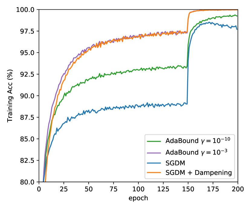
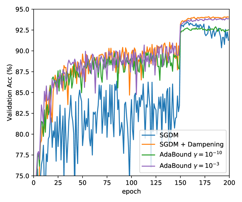
Figure 1: Training curves for AdaBound and momentum SGD (SGDM) (left: training accuracy, right: test accuracy) when optimizing a Wide ResNet 28-2 on the CIFAR-10 dataset. AdaBound suffers a significant performance drop both in training accuracy and final test performance with very small values of $\gamma$. Adding dampening ($\kappa=\beta_{1}$ instead of $\kappa=0$ in (24)) to SGDM yields a momentum update which matches AdaBound and other Adam-like methods, causing a dramatic performance increase (compare blue and orange curves) and providing performance similar to AdaBound (orange and purple curves).

6 Discussion

In this technical report, we identified issues in the proof of the main Theorem of Luo et al. (2019), which presents a regret rate guarantee for AdaBound. We presented an instance where the statement does not hold, and provided a $O(\sqrt{T})$ regret guarantee under different – and arguably less restrictive – assumptions. Finally, we observed empirically that AdaBound with a theoretically optimal $\gamma$ indeed yields superior performance, although it degenerates to a specific form of momentum SGD. Our experiments suggest that this form of SGDM (with a dampening factor equal to its momentum) performs competitively to AdaBound on CIFAR.

Acknowledgements

We are in debt to Rachit Nimavat for proofreading the manuscript and the extensive discussion, and thank Sudarshan Babu and Liangchen Luo for helpful comments.

References

• Cesa-Bianchi et al. (2006) N. Cesa-Bianchi, A. Conconi, and C. Gentile. On the generalization ability of on-line learning algorithms. IEEE Trans. Inf. Theor., September 2006.
• Devlin et al. (2018) Jacob Devlin, Ming-Wei Chang, Kenton Lee, and Kristina Toutanova. Bert: Pre-training of deep bidirectional transformers for language understanding. arXiv:1810.04805, 2018.
• DeVries & Taylor (2017) Terrance DeVries and Graham W Taylor. Improved regularization of convolutional neural networks with cutout. arXiv:1708.04552, 2017.
• Duchi et al. (2011) J. Duchi, E. Hazan, , and Y. Singer. Adaptive subgradient methods for online learning and stochastic optimization. ICML, 2011.
• He et al. (2016) Kaiming He, Xiangyu Zhang, Shaoqing Ren, and Jian Sun. Deep residual learning for image recognition. CVPR, 2016.
• Kingma & Ba (2015) Diederik P. Kingma and Jimmy Ba. Adam: A method for stochastic optimization. ICLR, 2015.
• Krizhevsky (2009) Alex Krizhevsky. Learning multiple layers of features from tiny images. Technical report, 2009.
• Luo et al. (2019) Liangchen Luo, Xiong, Yuanhao, Liu, Yan, and Xu. Sun. Adaptive gradient methods with dynamic bound of learning rate. ICLR (arXiv:1902.09843), 2019.
• Reddi et al. (2018) Sashank J. Reddi, Satyen Kale, and Sanjiv Kumar. On the convergence of adam and beyond. ICLR, 2018.
• Savarese et al. (2019) Pedro Savarese, David McAllester, Sudarshan Babu, and Michael Maire. Domain-independent Dominance of Adaptive Methods. arXiv:1912.01823, 2019.
• Tieleman & Hinton (2012) T. Tieleman and G. Hinton. Lecture 6.5—RmsProp: Divide the gradient by a running average of its recent magnitude. COURSERA: Neural Networks for Machine Learning, 2012.
• van den Oord et al. (2017) Aaron van den Oord, Oriol Vinyals, and Koray Kavukcuoglu. Neural Discrete Representation Learning. arXiv:1711.00937, 2017.
• Wilson et al. (2017) Ashia C. Wilson, Rebecca Roelofs, Mitchell Stern, Nathan Srebro, and Benjamin Recht. The Marginal Value of Adaptive Gradient Methods in Machine Learning. NIPS, 2017.
• Zagoruyko & Komodakis (2016) Sergey Zagoruyko and Nikos Komodakis. Wide residual networks. BMVC, 2016.
• Zinkevich (2003) Martin Zinkevich. Online convex programming and generalized infinitesimal gradient ascent. ICML, 2003.