The probability distribution of 3-D shapes of galaxy clusters from 2-D X-ray images

Abstract

We present a new method to determine the probability distribution of the 3-D shapes of galaxy clusters from the 2-D images using stereology. In contrast to the conventional approach of combining different data sets (such as X-rays, Sunyaev-Zeldovich effect and lensing) to fit a 3-D model of a galaxy cluster for each cluster, our method requires only a single data set, such as X-ray observations or Sunyaev-Zeldovich effect observations, consisting of sufficiently large number of clusters. Instead of reconstructing the 3-D shape of an individual object, we recover the probability distribution function (PDF) of the 3-D shapes of the observed galaxy clusters. The shape PDF is the relevant statistical quantity which can be compared with the theory and used to test the cosmological models. We apply this method to publicly available Chandra X-ray data of 89 well resolved galaxy clusters. Assuming ellipsoidal shapes, we find that our sample of galaxy clusters is a mixture of prolate and oblate shapes, with a preference for oblateness with the most probable ratio of principle axes 1.4 : 1.3 : 1. The ellipsoidal assumption is not essential to our approach and our method is directly applicable to non-ellipsoidal shapes. Our method is insensitive to the radial density and temperature profiles of the cluster. Our method is sensitive to the changes in shape of the X-ray emitting gas from inner to outer regions and we find evidence for variation in the 3-D shape of the X-ray emitting gas with distance from the centre.

1 Introduction

It has long been known that non-linear gravitational collapse in the matter dominated Universe, starting with Gaussian random field initial conditions, happens non-spherically, giving rise to Zeldovich pancakes, filaments and galaxy clusters (Zeldovich, 1970; Shandarin & Zeldovich, 1989), and creating the cosmic web which has been detected in observations (Geller & Huchra, 1989; Colless et al., 2001; Gott et al., 2005) as well as simulations (Klypin & Shandarin, 1983; Davis et al., 1985; Springel et al., 2005). In particular, we expect that galaxy clusters, the largest collapsed objects in the Universe at the intersection of filaments, will also not be perfectly spherical (Frenk et al., 1988a). Observationally we know that the galaxy clusters are not spherical since their 2-D projections are not circular in optical (Carter & Metcalfe, 1980; Binggeli, 1982), X-ray (Fabricant et al., 1984; Buote & Canizares, 1992, 1996; Kawahara, 2010), Sunyaev-Zeldovich (SZ) effect (Sayers et al., 2011), weak gravitational lensing (Evans & Bridle, 2009; Oguri et al., 2010; Oguri et al., 2012) and strong gravitational lensing (Soucail et al., 1987) data. Further evidence for asphericity of galaxy clusters comes from kinematics of galaxies in the clusters (Skielboe et al., 2012).

Cold dark matter simulations show correlations between the orientations of dark matter halos and the surrounding cosmic web (van Haarlem & van de Weygaert, 1993; Splinter et al., 1997; Kasun & Evrard, 2005; Bailin & Steinmetz, 2005; Altay et al., 2006; Patiri et al., 2006; Aragón-Calvo et al., 2007; Brunino et al., 2007). Taking asphericity into account is also important for accurate mass determinations of the galaxy clusters (Piffaretti et al., 2003; Clowe et al., 2004; Gavazzi, 2005; Corless & King, 2007; Battaglia et al., 2012; Green et al., 2019; Chen et al., 2019) which in turn is important for using the galaxy clusters for precision cosmology (Mantz et al., 2015; Planck Collaboration et al., 2016; de Haan et al., 2016). The shape of the galaxy cluster will also be influenced by the nature of dark matter, for example the self interactions of the dark matter (Peter et al., 2013). The future X-ray (Merloni & German eROSITA Consortium, 2012) and Sunyaev-Zeldovich effect surveys (K. N. Abazajian et al., 2016) will yield hundreds of thousands of galaxy clusters making precision cosmology with statistics of cluster shapes feasible. The shape of galaxy clusters is therefore emerging as an important observable which can be used to test the $\Lambda$CDM cosmology, baryonic physics in the intracluster medium (ICM) and fundamental physics such as the nature of dark matter.

One of the obstacles to using galaxy cluster shapes as a cosmological probe is the fact that we have only 2-D information about these objects. The X-ray and SZ effect (Zeldovich & Sunyaev, 1969; Sunyaev & Zeldovich, 1972) observations give us 2-D images in X-ray and microwave bands. The optical galaxy surveys also do not give us 3-D information since for most galaxies we do not have absolute distance measurements but only the redshifts. We can therefore only infer the average distance of the cluster in a cosmological model but not the distances to the individual galaxies. Gravitational lensing is also mostly sensitive to the 2-D projected mass distribution. Therefore, before we can use cluster shapes as a cosmological probe, we must solve the problem of inferring 3-D shape of the clusters from 2-D data.

Previously, inference of 3-D shapes of galaxy clusters, without assuming spherical or axial symmetry, has been tried by combining many different probes such as X-ray and SZ (Lee & Suto, 2004) with lensing data (Limousin et al., 2013), using X-ray spectra (Samsing et al., 2012) and using weak and strong lensing data (Chiu et al., 2018). We propose a new method to infer the distribution of 3-D shapes of galaxy clusters. Our method adds a new tool to the existing toolkit for 3-D shape inference and can serve as an independent check of the results obtained by other methods. Our method is relatively computationally inexpensive and well suited to be applied to large data sets of hundreds of thousands of clusters that will become available with the future SZ and X-ray surveys. As we will see, our method does not need the galaxy clusters or the gas distribution to be ellipsoidal but can handle more general geometries. We will however make the ellipsoidal assumption in this paper for simplicity and also to compare our results with the published results in literature. Similar method has been used by Makarenko et al. (2015) to study the neutral hydrogen gas distribution in the turbulent interstellar medium of the Milky Way.

2 Stereology of galaxy clusters

The field of Stereology combines the ideas of Geometry and Statistics to obtain information about the 3-D shapes of objects from a small number of 2-D projections or cross-sections (Baddeley & Jensen, 2004). This approach lends itself naturally to astrophysics where we usually have a single 2-D image or a projection of each of a large number of astrophysical objects belonging to a particular class or population and we want to infer the collective 3-D properties of the population. Following Makarenko et al. (2015), we use the probability distribution of filamentarity (F), a quantity constructed from Minkowski Functionals, to solve the deprojection problem.

In two dimensions, the morphological properties of any 2-D contour can be completely characterized by three Minkowski Functionals. More generally, in $n$ dimensions there are $n+1$ Minkowski functionals, a result known as Hadwidger’s theorem (Hadwiger, 1957; Schmalzing et al., 1996). These three Minkowski Functionals are enclosed area $S$, perimeter $P$ and Euler Characteristic of the contour. We will work with simple closed contours (with Euler characteristic $=0$) so that the only Minkowski functionals with non-trivial information are the area and the perimeter. We can further combine the perimeter and area to form a quantity called Filamentarity $F$, which is defined as (e.g. see Bharadwaj et al., 2000):

$$F=\frac{P^{2}-4\pi S}{P^{2}+4\pi S}.$$ (1)

This definition ensures that $0\leq F\leq 1$ with $F=0$ corresponding to a circle and $F\rightarrow 1$ in the limit $S\rightarrow 0$ i.e. a line segment. When the circle is stretched to an ellipse of increasingly higher eccentricity, its filamentarity keeps increasing. The line segment with the limiting value of $F=1$ is not necessarily straight. It should be noted that instead of filamentarity, we can also use ellipticity as a shape descriptor if we confine ourselves to ellipsoidal shapes. We will use filamentarity keeping in mind future applications where we may want to consider non-ellipsoidal shapes.

Let us assume that a galaxy cluster is an ideal ellipsoid with length $L$, width $W$ and thickness $T$ ($L>W>T$). To constrain the shape, we need to determine the ratio $L:W:T\equiv\ell:w:1$, where we have defined $\ell=L/T$ and $w=W/T$. We will work with the ratios $\ell$ and $w$, since we are not interested in overall size of the cluster but only its shape. We will first consider a large sample (sample size $\sim 150,000$ clusters) of isotropically oriented ellipsoids (galaxy clusters) with same shape ($\ell$ and $w$) or equivalently observe the same galaxy cluster from a large number of random observer positions. We use a simple theoretical model for X-ray emission in a galaxy cluster and use it to generate the theoretical X-ray surface brightness map for a given orientation of the cluster. We should emphasize that that our method is not sensitive to the detailed modelling of the cluster, in particular the density and temperature profiles as a function of distance from the centre, but only the 3-D shape of the cluster. We show this model independence explicitly below. We obtain the isocontours of constant X-ray intensity from this X-ray surface brightness map and use them to calculate the filamentarity. Finally, we repeat this for all the clusters of the sample to obtain the Probability Distribution Function (PDF) of filamentarity, ${{\mathcal{P}}}(F|\ell,w)$ for a given $\ell$ and $w$. Comparing the filamentarity PDF of X-ray images with the theoretical PDFs of different $\ell$ and $w$ then gives us information about the population of observed galaxy clusters. Note that by definition, $L\geq W\geq T$ or $\ell\geq w\geq 1$. In particular, $\ell\approx w>1$ corresponds to an oblate spheroid while $\ell>w\approx 1$ corresponds to a prolate spheroid and $\ell\approx w\approx 1$ is a spherical shape.

2.1 The X-ray emission model for galaxy clusters

In galaxy clusters, with typical temperatures $T\approx 10^{7}-10^{8}$ K, the primary emission process is thermal bremsstrahlung (free-free) emission. The total power emitted per unit volume (emissivity integrated over frequency) is given by (Rybicki & Lightman, 1979):

$$\epsilon=\sum_{i}\left(\frac{2\pi{{k_{\rm B}}}}{3m}\right)^{\frac{1}{2}}\frac{2^{5}\pi e^{6}}{3hmc^{3}}Z_{i}^{2}{{n_{\rm e}}}n_{i}T^{\frac{1}{2}}\bar{g}~{}\propto\sum_{i}Z_{i}^{2}{{n_{\rm e}}}n_{i}T^{\frac{1}{2}}$$ (2)

where $m$ is the mass of electron, ${{n_{\rm e}}}$ and $n_{i}$ are the number densities of electrons and ions of species $i$ respectively, $Z_{i}$ the corresponding charge, $T$ is the electron temperature and $\bar{g}$ is the frequency averaged Gaunt factor ($\bar{g}\sim 1.2$), ${{k_{\rm B}}}$ is the Boltzmann constant, $e$ is the charge of the electron, $h$ is the Planck constant, and $c$ is the speed of light. Assuming charge neutrality and uniform abundance of elements throughout the cluster gives $\sum_{i}Z_{i}^{2}n_{i}\propto{{n_{\rm e}}}$ and therefore we can write the X-ray surface brightness $S_{X}$ as integral of the emissivity over the line of sight distance $z$,

$$S_{X}=\int\epsilon~{}{{{\rm d}}}z\propto\int{{n_{\rm e}}}^{2}T^{\frac{1}{2}}{{{\rm d}}}z$$ (3)

We assume a generalized triaxial Navarro, Frenk & White (NFW) model (Navarro et al., 1996; Jing & Suto, 2002) to represent the electron density ${{n_{\rm e}}}\propto\rho(R)$ of the cluster as

$$\rho(R) =\frac{\rho_{c}}{\left(\frac{R}{R_{S}}\right)^{\gamma}\left(1+\frac{R}{R_{S}}\right)^{3-\gamma}},$$ (4)

$$R^{2} \equiv L^{2}\left(\frac{x^{2}}{L^{2}}+\frac{y^{2}}{W^{2}}+\frac{z^{2}}{T^{2}}\right),$$ (5)

where $x,y,z$ are the coordinates with origin at the centre of the cluster and $R=L$ defines the outer boundary of the cluster upto which we integrate the X-ray flux along the line of sight. Since most of the X-ray flux is contributed by high density regions, the integral converges quickly and we do not need to integrate out to a great distance from the cluster centre along the line of sight. Also, we are not interested in absolute magnitude of brightness but only the shapes of the isocontours in an X-ray image. We have explicitly checked that the shapes of isocontours, and hence our results, are not sensitive to how far out we integrate as long as we integrate to a distance greater than the scale radius $R_{S}$. We fix the values $\rho_{c}=1$, $\gamma=1$, and $R_{S}=1$ in arbitrary units. The profile of electron density (Vikhlinin et al., 2006) usually differs from the dark matter profile which the NFW model represents. Our observable, the filamentarity, which captures only the shape information is relatively insensitive to the exact density profile of gas. We check this explicitly below by using different electron and temperature density profiles from Vikhlinin et al. (2006) obtained from the X-ray observations of different galaxy clusters. This relative insensitivity to the exact density profile is an advantage in our method compared to other methods relying on the complete 3-D modelling of the cluster.

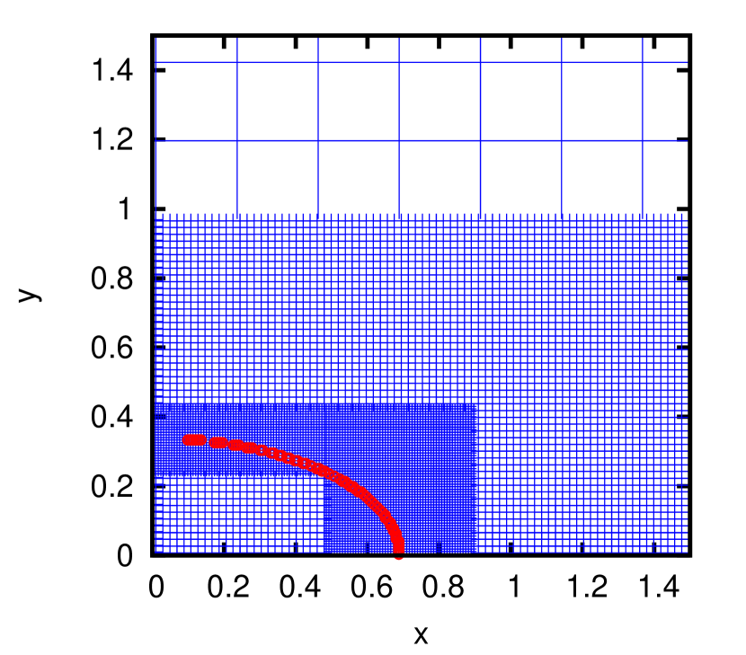
Figure 1: Adaptive refinement search for the isocontours: We start with an initial low resolution grid ($\Delta x=\Delta y=2.26\times 10^{-1}$ in this example). We refine the grid several times, each time increasing the resolution close to the desired isocontour, which in turn refines the isocontour. After a few refinements, we get the isocontour at high resolution ($\Delta x=\Delta y=7.48\times 10^{-3}$).

We take a universal temperature profile for galaxy clusters (Loken et al., 2002):

$$T(R)\propto[1+R/a_{R}]^{-\delta};\qquad a_{R}=1,\qquad\delta=1.6\,.$$ (6)

To generate the X-ray surface brightness map, we start with a uniform grid in the XY plane. We rotate the grid so that the normal to the plane of this grid is aligned with the line of sight direction $\hat{k}$. For every point on the rotated plane, we calculate the integral $S_{X}$ for X-ray intensity using Eq.3. We then rotate the plane back to the XY-plane. This gives the X-ray surface brightness map in the XY plane for an arbitrary orientation (given by line of sight direction $\hat{k}$) of the observer with respect to the cluster. To obtain the isocontours in a computationally efficient manner we do adaptive refinement of the grid. We start with an initial coarse grid and follow the above steps several times, each time successively increasing the resolution in the region close to the desired isocontour. After a small number of refinements, we have the isocontour sampled at high resolution. This is illustrated in Fig.1. We fit the points on the isocontour with an ellipse using Downhill-simplex algorithm (Nelder & Mead, 1965). The filamentarity of the resultant ellipse can be easily calculated using Eq. 1 with $S=\pi ab$ and $P$ given with better than a percent accuracy by (Lidstone, 1932)

$$P\approx\pi(a+b)\frac{1-3\lambda^{4}/64}{1-\lambda^{2}/4},\ \ \lambda=\frac{a-b}{a+b},$$ (7)

where $a$ and $b$ are semi-major and semi-minor axes of the ellipse respectively.

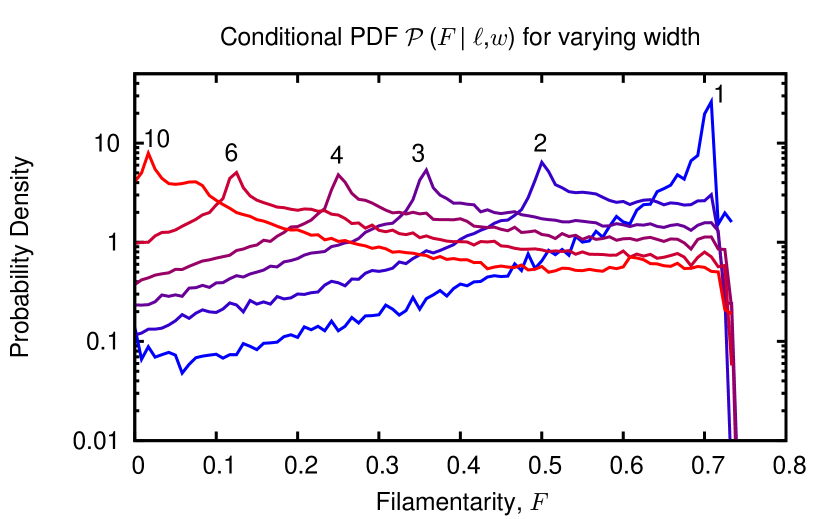
Figure 2: Conditional filamentarity PDFs, ${{\mathcal{P}}}(F|\ell,w)$, for $\ell=16$ and $w\in\{1,2,3,4,6,10\}$. The PDF has been obtained using $\approx 150,000$ isotropic random projections binned into 120 intervals of $F$ between $[0,1]$. The labels refer to the values of $w$. It can be seen that peak filamentarity($F_{p}$) decreases with increase in $w$.

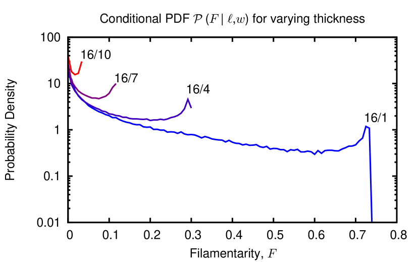
Figure 3: Conditional filamentarity PDFs, ${{\mathcal{P}}}(F|\ell,w)$, for $\ell=w\in\{16,16/4,16/7,16/10\}$. The PDF has been obtained using $\approx 150,000$ isotropic random projections binned into 120 intervals of $F$ between $[0,1]$. The labels refer to the values of $\ell=w$. It can be seen that cut-off filamentarity ($F_{c}$) increases with increase in $\ell,w$.

2.2 Filamentarity PDF and its model independence

By observing a cluster from random directions, we can build up the probability distribution function of the filamentarity that a random observer would measure. The filamentarity PDF for a fixed $\ell\equiv L/T$ and $w\equiv W/T$, ${{\mathcal{P}}}(F|\ell,w)$, depends on the value of $\ell,w$ of the cluster. Equivalently, if we observe single images of large number of clusters, all of which have the same $\ell$ and $w$, then this is the PDF we will get. The PDF is characterized by a sharp peak (Peak Filamentarity, $F=F_{p}$) and a sharp cut-off (Cut-off Filamentarity, $F=F_{c}$) which are functions of $\ell$ and $w$. If $L$ and $T$ are kept constant (i.e. $\ell$ constant and varying $w$), $F_{p}$ decreases non-linearly with an increase in $W$. This is illustrated in Fig. 2. On the other hand, if $L$ and $W$ are kept constant (i.e. $\ell$ and $w$ changing by the same factor), $F_{c}$ decreases with an increase in $T$ as seen in Fig. 3 . In reality, we expect different clusters to have different $\ell$ and $w$ and the observed filamentarity PDF, ${{\mathcal{P}}}(F)$, would be a superposition of conditional PDFs for different $\ell$ and $w$,

$${{\mathcal{P}}}(F) =\int{{{\rm d}}}\ell{{{\rm d}}}w{{\mathcal{P}}}(F,\ell,w)$$

$$=\int{{{\rm d}}}\ell{{{\rm d}}}w{{\mathcal{P}}}(F|\ell,w){{\mathcal{P}}}(\ell,w),$$ (8)

where ${{\mathcal{P}}}(\ell,w)$ is the PDF of shapes of clusters and ${{\mathcal{P}}}(F,\ell,w)$ is the joint PDF. Our goal is to recover the PDF of shapes, ${{\mathcal{P}}}(\ell,w)$.

We have used a simple model for the profiles of electron density and temperature. Since we are interested in only the shapes of the isocontours of X-ray surface brightness and not their overall amplitudes, our results are not sensitive to the exact profile. To test this hypothesis, we repeat the calculation using two different density and temperature profiles from Vikhlinin et al. (2006) and compare it with our NFW + universal temperature profile model in Fig. 4. As we can see, there is negligible change (less than the Monte Carlo noise) in the PDF of filamentarity confirming our assertion that the filamentarity PDF is sensitive only to the shape of the cluster.

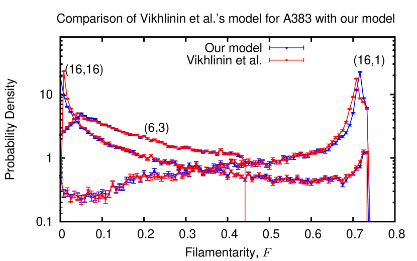
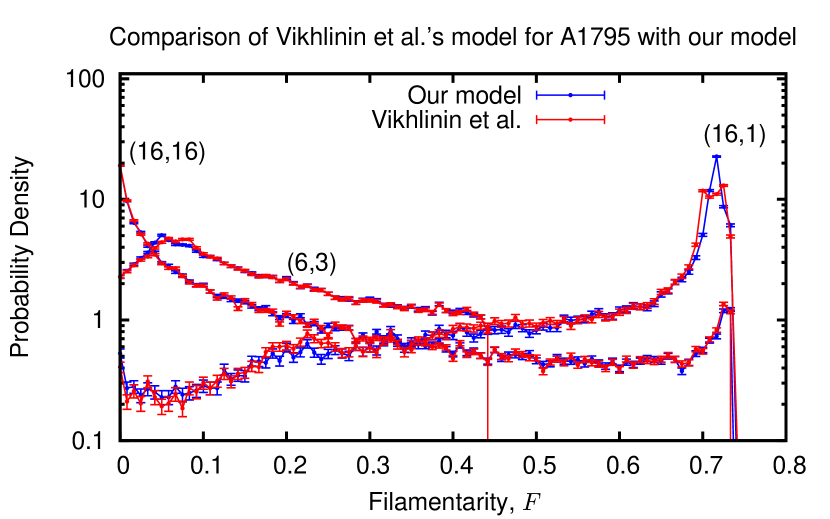
Figure 4: Comparison of our NFW + universal temperature profile model with temperature and density profile models from Vikhlinin et al. (2006), for two clusters with very different parameter values: A383 and A1795. We have made the comparison for three different shapes: one prolate ($\ell=w=16$), one oblate ($\ell=16,w=1$) and one intermediate ($\ell=6,w=3$) shape. We find a general agreement of our model with that of Vikhlinin et al. (2006), differences being less than the Monte Carlo noise.

3 Filamentarity PDF of Chandra X-ray clusters

The next step is to obtain the PDF of filamentarity of isocontours of X-ray surface brightness maps from observational data. We use the X-ray data of 89 galaxy clusters from the catalogue compiled by Eric Tittley from the Chandra Data Archive (Chaser) for this purpose. We start by selecting an initial sample of galaxy clusters which have the ratio of X-ray counts at the cluster center/peak to the background greater than or equal to 3. We manually check the cluster metadata to see if they are explicitly mentioned to be merging. We do not include these merging clusters in our sample. We use the already processed full image data for our analysis. We do not reprocess the data because reprocessing only changes the calibration, which will not affect the shape of the isocontours. The list of galaxy clusters used in this paper is given in Appendix B. We should point out that we are not trying to find an average cluster shape or fit a single shape to all clusters. We are inferring the full probability distribution function of the cluster shapes, ${{\mathcal{P}}}(\ell,w)$. Therefore selection of clusters based on cluster physics or any other criteria a priori is not needed. In particular, for example, if there are two (or more) populations of clusters with distinct shapes, our method would result in two (or more) distinct peaks in the shape PDF, ${{\mathcal{P}}}(\ell,w)$. We should note that there may be large selection effects and we should be careful that our selection criteria does not remove the population that we are interested in studying. In our analysis, we explicitly remove the merging clusters. A merging cluster can also be roughly approximated as an elongated ellipsoid and we would expect that the shape PDF would broaden towards highly elongated shapes if these clusters were included. A modification of our algorithm would be required to model merging clusters more accurately, since they may depart significantly from the ellipsoidal shape. Such a modification would be non-trivial but possible since filamentarity is defined even for non-elliptical shapes.

For a given cluster, we subtract the background and carry out convolution of the resultant data using a Gaussian function with the standard deviation $\sigma=3$ pixels to smooth the image and suppress noise. After convolution, we obtain the isocontours corresponding to a given X-ray count and fit it with an ellipse using the Downhill-simplex algorithm. We then do a binary search by looking at isocontours corresponding to larger or smaller X-ray counts until we find the isocontour which encloses the desired fraction of X-ray flux. This algorithm works because the enclosed X-ray flux increases monotonically and X-ray counts decrease monotonically as we move away from the centre of the cluster. In this work, we choose isocontours which enclose 25%, 40%, 60%, 80% and 90% of the total flux respectively. These isocontours laid on top of the X-ray flux maps of Chandra clusters A1835 and A2204 are shown in Fig. 5. We calculate the filamentarity of the best-fit ellipse using Eq. 1 and Eq. 7. We repeat these steps for 89 clusters to get 89 values of filamentarity, which are then binned to obtain the PDFs which are shown in Fig. 6. During this analysis, we have neglected the isocontours which are very distorted from elliptical shape. We neglect them because these isocontours are so distorted that an attempt to fit an ellipse fails for them. This is the reason for the lower sample size when we go to isocontours of higher percent enclosed flux, because the distortion from elliptical shape is more for them. We see from Fig. 6 that the ellipticity of the clusters is small with the maximum filamentarity smaller than $\sim 0.15$. We have binned $F$ with a bin-width of $1/120$ and we also show the Poisson error bars. There is a difference in the tails of the PDFs, indicating that there is a variation in shape as we go from inner part of the cluster to the outer parts.

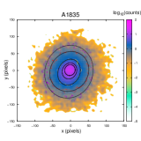
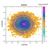
Figure 5: Smoothed X-ray surface brightness maps of Chandra clusters A1835 and A2204. The X-ray count is in log scale. The best-fitting isocontours of X-ray counts (in black color) for 25%,40%,60%,80% and 90% enclosed flux are shown, along with the fit points.

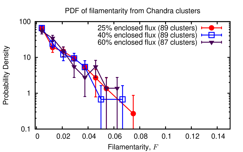
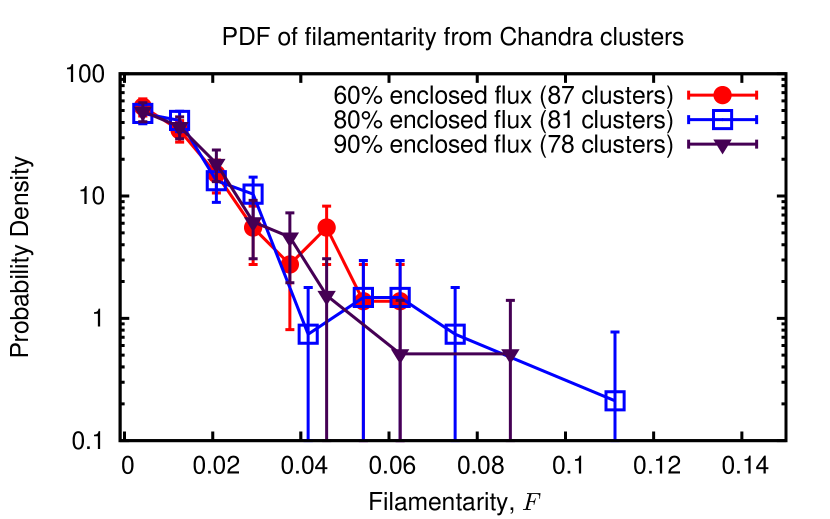
Figure 6: PDF of filamentarity, ${{\mathcal{P}}}_{\rm obs}(F)$, from Chandra X-ray clusters, obtained using up to 89 clusters and binned with a bin-width of $1/120$ in $F$. We calculate the PDF separately for the isocontours enclosing 25%, 40%, 60%, 80% and 90% of flux. The PDF for 80% and 90% flux has been obtained using $81$ and $78$ clusters respectively, instead of $89$, since the shapes of isocontours on the outer parts of a few clusters deviate considerably from the elliptical shape due to noise. The five PDF’s are similar at lower values of $F$ ($F_{p}\approx 0$ and $F_{c}\approx 0.06$-$0.13$), with differences in the tail of the curves at larger values of $F$.

3.1 Results for shapes of Chandra X-ray clusters

Our goal is to recover the shape PDF, ${{\mathcal{P}}}(\ell,w)$. To this end, we can bin the shape PDF in bins of $\ell,w$ and thus reconstruct a discretized form of ${{\mathcal{P}}}(\ell,w)$. This is equivalent to approximating ${{\mathcal{P}}}(\ell,w)$ by a superposition of Dirac delta distributions,

$${{\mathcal{P}}}(\ell,w) \approx\sum_{i=1}^{n}a_{i}\delta_{D}\left(\ell-\ell_{i},w-w_{i}\right)$$ (9)

with the normalization condition,

$$\sum_{i=1}^{n}a_{i} =1.$$ (10)

Substituting it in Eq. 8, we get after integrating out the Dirac delta distributions,

$${{\mathcal{P}}}(F)\approx\sum_{i=1}^{n}a_{i}{{\mathcal{P}}}(F|\ell_{i},w_{i})$$ (11)

Our problem of finding the shape PDF now reduces to finding the number of bins $n$, the bin centres $\ell_{i},w_{i}$ and the relative probability amplitudes of different shapes $a_{i}$ which best fit the data.

In order to proceed, we generate 100 random values of $(\ell,w)$ taken from a uniform distribution. By definition, $\ell\geq w\geq 1$. Hence, we take the value of $\ell$ from a uniform random distribution $[1,2.6]$ and the value of $w$ from a uniform random distribution $[1,\ell]$. The upper limit for $\ell$, $2.6$, corresponds to $F_{c}\approx 0.15$ and therefore covers the observed range of $F$. We generate the conditional PDFs, ${{\mathcal{P}}}(F|\ell,w)$, for each of the 100 randomly sampled ($\ell,w$). This is sufficient for the present paper since we are limited by the small size of our data sample.

For each $w_{i},\ell_{i}$ combination for a given $n$, we therefore find the best-fitting values of ($a_{1},a_{2},....,a_{n-1}$) by minimizing the following $\chi^{2}$:

$$\chi^{2}=\sum\limits_{j}\frac{[{{\mathcal{P}}}(F_{j})-{{\mathcal{P}}}_{obs}(F_{j})]^{2}}{\sigma_{j}^{2}}$$ (12)

where $F_{j}$ is the $jth$ bin and $\sigma_{j}$ is the Poisson error in the corresponding bin given by $\sigma_{j}=(\sqrt{n_{\rm obs}(j)}/n_{\rm total})\times n_{\rm bin}$, where $n_{\rm obs}$ is the observed count in that bin, $n_{\rm total}$ is the total number of clusters in the data set and $n_{\rm bin}$ is the total number of bins of filamentarity.

We first consider the simplest model that all clusters have the same shape, i.e. $n=1$. The Observational PDF has $F_{p}\approx 0$ and $F_{c}\approx 0.06-0.13$, depending on the per cent flux enclosed. We vary $w_{1},\ell_{1}$ to find the ${{\mathcal{P}}}(F|w_{1},\ell_{1})$ that best fits the observed ${{\mathcal{P}}}(F)$. However, the lowest $\chi^{2}/d.o.f$ for this model comes out to be $\approx 1.5-3.5$, which is not satisfactory. Thus, we see immediately that the shapes of the galaxy clusters must vary from cluster to cluster.

We next perform a $\chi^{2}$-fitting of $\mathcal{P}(F)$ to the observed PDF by fitting the $n-1$ variables $a_{i}$ for each combination of $w_{i},\ell_{i}$ for different $n$, starting with $n=2$ and choose the combination $w_{i},\ell_{i}$ that gives the least $\chi^{2}$. Note that one of the $a_{i}$ is fixed by the normalization condition, $\sum_{i}a_{i}=1$. We are therefore doing a model selection, with different $w_{i},\ell_{i},n$ corresponding to a different model for ${{\mathcal{P}}}(F)$, while $a_{i}$ are the parameters of the model which are being fit for each model. Our model selection consists of a brute force search for the best-fitting $w_{i},\ell_{i}$ by repeating the fit for every possible set of $\ell_{i},w_{i}$. Thus, we have a total of ${}^{100}C_{n}$ combinations to fit. We find the $\chi^{2}$ for each of these sets and take the combination with the minimum value $\chi^{2}_{\rm min}$ as the best-fitting model. We repeat the whole procedure for $n=2,3,4$ and find $\chi^{2}_{\rm min}$ in each case. It should be noted that during the fitting procedure for a given $n$, we only accept those combinations of {($\ell_{i},w_{i}$) $i=1,n$} which satisfy the condition that $F_{c}$ for at least one $\mathcal{P}(F|\ell_{i},w_{i})$ $\geq$ $F_{c}$ for $\mathcal{P}_{obs}(F)$. The results are tabulated in Table 1.

To summarize, our method is accomplishing three things simultaneously:

1. We find the optimal number of bins, $n$, demanded by the data into which to divide the filamentarity PDF, ${{\mathcal{P}}}(F)$.

2. For each $n$, we find the best-fitting model corresponding to different values of $\{\ell_{i},w_{i}\}$.

3. For each model we find the best-fitting parameters $a_{i}$ by solving the linear minimization problem.

$n$	$\chi_{\rm min}^{2}/d.o.f$
	$25\%$ flux	$40\%$ flux	$60\%$ flux	$80\%$ flux	$90\%$ flux
1	3.55	3.99	1.85	1.19	1.32
2	1.19	2.61	0.43	0.80	0.46
3	0.13	0.07	0.26	0.10	0.02
4	0.01	0.008	0.19	0.09	0.005

Table 1: The variation of $\chi^{2}_{min}/d.o.f$ when Observational PDF ($\mathcal{P}_{obs}(F)$) at different enclosed intensities ($25\%$, $40\%$, $60\%$, $80\%$ and $90\%$) is fit with the theoretical PDF ($\mathcal{P}(F)$) for $n=1,2,3,4$. Degree of Freedom, $d.o.f=d-p$, where $d$ is the number of non-zero data points and $p$ is the number of independent parameters. $\chi^{2}_{min}/d.o.f$ becomes $\lesssim 1$ at $n=2$ for all the cases of different enclosed X-ray flux. For 40% flux case, $\chi^{2}_{min}/d.o.f$ is $0.07\ll 1$ for $n=3$, which is a sign of overfitting, hence we choose the result for $n=2$ for this case also.

We observe that $\chi^{2}/d.o.f$ decreases progressively from $n=1$ to $n=4$, for each enclosed per cent flux. However, $\chi^{2}/d.o.f$ becomes $\lesssim 1$ in every case for $n=2$. This means that $n=2$ is the optimal number of parameters. Thus, a superposition of $2$ cluster shapes is adequate to describe the data. The best-fitting parameters and model for $n=2$ is shown in Table 2 and Fig.7.

We can define a triaxiality parameter $\mathcal{T}$ to classify the shapes of the clusters:

$$\mathcal{T}=\frac{L^{2}-W^{2}}{L^{2}-T^{2}}=\frac{\ell^{2}-w^{2}}{\ell^{2}-1}$$ (13)

For a purely oblate shape, $L=W$ or $\mathcal{T}=0$. For a purely prolate shape, $W=T$ or $\mathcal{T}=1$. We classify the shapes as nearly oblate $(0<\mathcal{T}\lesssim 0.33)$, triaxial $(0.33\lesssim\mathcal{T}\lesssim 0.67)$ or nearly prolate $(0.67\lesssim\mathcal{T}<1)$ (Warren et al., 1992). The results of this classification are shown in Table 3. We see that the higher-weighted shape is prolate for the innermost part while it has preference towards oblateness for the outer parts. Lower-weighted shape is prolate in the inner parts and triaxial in the outer parts.

Enclosed flux	$\ell_{1}$	$w_{1}$	$a_{1}$	$\ell_{2}$	$w_{2}$	$a_{2}$
25%	1.24	1.07	$0.55\pm 0.13$	1.81	1.34	0.45
40%	1.33	1.24	$0.74\pm 0.12$	1.80	1.25	0.26
60%	1.41	1.30	$0.75\pm 0.14$	1.99	1.62	0.25
80%	1.41	1.30	$0.84\pm 0.12$	2.04	1.52	0.16
90%	1.41	1.30	$0.81\pm 0.14$	1.97	1.51	0.19

Table 2: The best-fitting parameters and model for $n=2$ fit for $25\%$, $40\%$, $60\%$, $80\%$ and $90\%$ enclosed flux. $a_{j}$ represents the probability of corresponding $(\ell_{j},w_{j})$ in the joint PDF $\mathcal{P}(F,\ell,w)$ (Eq. 8). The error on $a_{2}$ is the same as that of $a_{1}$, since $a_{2}=1-a_{1}$.

Flux	$(\ell_{1},w_{1})$	$\mathcal{T}_{1}$	$(\ell_{2},w_{2})$	$\mathcal{T}_{2}$
25%	(1.24,1.07)	$0.73$ (prolate)	(1.81,1.34)	$0.65$ (prolate)
40%	(1.33,1.24)	$0.30$ (oblate)	(1.80,1.25)	$0.75$ (prolate)
60%	(1.41,1.30)	$0.30$ (oblate)	(1.99,1.62)	$0.45$ (triaxial)
80%	(1.41,1.30)	$0.30$ (oblate)	(2.04,1.52)	$0.58$ (triaxial)
90%	(1.41,1.30)	$0.30$ (oblate)	(1.97,1.51)	$0.55$ (triaxial)

Table 3: Same as Table 2, but showing the shape classification of the clusters as prolate, triaxial or oblate.

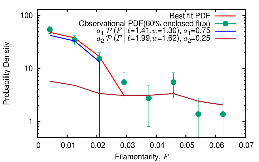
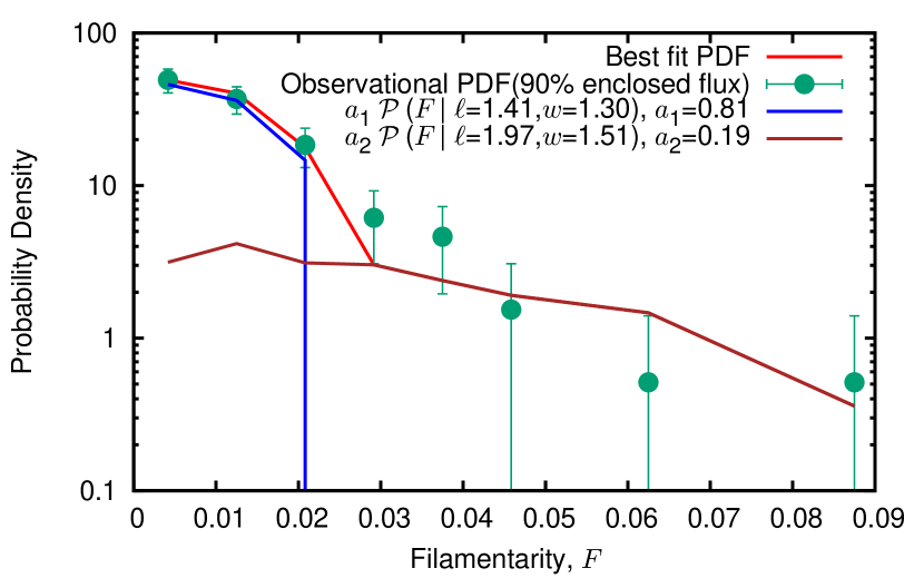
Figure 7: The comparison of Observational PDF $(\mathcal{P}_{obs})$ , best fit PDF $\mathcal{P}(F)$ as well as the two conditional PDFs $\mathcal{P}(F|\ell_{i},w_{i})$, for $60\%$ and $90\%$ enclosed flux. We also mention the weights $a_{i}$ in the legend. The shape $(\ell=1.41,w=1.30)$ contributes to the low $F$ part of both PDFs, while $(\ell=1.99,w=1.62)$ and $(\ell=1.97,w=1.51)$ contribute to the tail of the distribution for the PDF of $60\%$ and $90\%$ enclosed flux respectively.

3.2 Monte Carlo estimation of the shape PDF, ${{\mathcal{P}}}(\ell,w)$

In this section we use Monte Carlo sampling to get the shape PDF, ${{\mathcal{P}}}_{\ell,w}$.

We generate 4000 random values of $(\ell,w)$ taken from a uniform distribution. As before, for $\ell$ we have the uniform random distribution $[1,2.6]$ and for $w$ the uniform random distribution $[1,\ell]$. We generate the conditional PDFs, ${{\mathcal{P}}}(F|\ell,w)$, for each of the 4000 randomly sampled ($\ell,w$). We want to arrive at a Monte Carlo estimate of ${{\mathcal{P}}}(\ell,w)$ with the density of points in $\ell,w$ plane $\propto{{\mathcal{P}}}(\ell,w)$. To accomplish this, we start with the Uniform distribution. If the shape PDF was really Uniform, we should have the filamentarity distribution ${{\mathcal{P}}}(F)$ given by:

$${{\mathcal{P}}}(F)=\sum_{i=1}^{4000}a_{i}{{\mathcal{P}}}(F|\ell_{i},w_{i})\qquad\qquad a_{i}=1/4000$$ (14)

We calculate the $\chi^{2}$ between ${{\mathcal{P}}}(F)$ and ${{\mathcal{P}}}_{obs}(F)$ using Eq. 12. Next, we randomly choose 1 point out of the 4000 points which is removed and calculate the new PDF as:

$${{\mathcal{P}}}_{new}(F)=\sum_{i=1}^{3999}a_{i}{{\mathcal{P}}}(F|\ell_{i},w_{i})\qquad\qquad a_{i}=1/3999$$ (15)

We calculate $\chi_{new}^{2}$ between ${{\mathcal{P}}}_{new}(F)$ and ${{\mathcal{P}}}_{obs}(F)$. We accept or reject the change of removing the chosen point using the following condition :

• If($\chi^{2}_{new}\leq\chi^{2}$): we accept the change and remove the selected point from the sample set.

• If($\chi^{2}_{new}>\chi^{2}$): we reject the change and do not remove the selected point from sample set.

We repeat this procedure for many iterations. At each iteration, we calculate the PDF as:

$${{\mathcal{P}}}(F)=\sum_{i=1}^{n_{d}}a_{i}{{\mathcal{P}}}(F|\ell_{i},w_{i})\qquad\qquad a_{i}=1/n_{d}$$ (16)

where $n_{d}$ is the number of points remaining in the sample set. We stop the procedure when $\chi^{2}$ converges. Removing a point gives higher weightage to the remaining points. The density of points remaining in our Monte Carlo sample set is the best estimate of the shape PDF, ${{\mathcal{P}}}(\ell,w)$.

We started with a uniform distribution of points in the $(\ell,w)$ plane. After convergence, we have $\sim 100$ points non-uniformly distributed in the $(\ell,w)$ plane. The density of points at different places in the plane gives a measure of probability. It should be noted that in this method, the weight factor $a_{i}$ has been kept uniform throughout the calculation. Instead, the density of points per unit area has been used as a measure of probability. We divide the $\ell,w$ plane into bins of size $0.053\times 0.053$. The probability density at each bin center, $\ell_{j},w_{j}$, for each bin $j$ is calculated as:

$${{\mathcal{P}}}(\ell_{j},w_{j})=k(n_{j}^{\rm{final}}/n_{j}^{\rm{initial}})/A_{j}$$ (17)

where $A_{j}$ is a patch of square-shaped area around ($\ell_{j},w_{j}$), $n_{j}^{\rm{initial}}$ is the number of points inside area $A_{j}$ of each square bin initially, $n_{j}^{\rm{final}}$ is the number of points inside $A_{j}$ after convergence at the end of Monte Carlo and $k$ is the normalization constant such that $\sum_{j}{{\mathcal{P}}}(\ell_{j},w_{j})A_{j}=1$. The results are shown in the form of colour maps for the 2-d PDF in ($\ell,w$) plane in Fig. 8 and 9.

From these figures, we see that the shapes are predominantly spherical in the innermost parts of a galaxy cluster, with a preference towards prolateness. However, as we go to the outer parts of the cluster, the peak shifts and the most probable shape becomes triaxial, with a preference towards oblateness. These results agree well with the results obtained in the previous section. Note that the small number of points remaining at convergence is just due to the fact that our sample size is small.

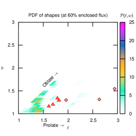
Figure 8: 2-D probability density of shapes in the ($\ell,w$) plane obtained using the Monte Carlo method, for 25%, 40% and 60% enclosed flux. The 4 red triangles and 3 brown diamonds correspond to the shapes of individual clusters obtained by Limousin et al. (2013) and Chiu et al. (2018) respectively. The probability density has been calculated for discrete ($\ell_{j},w_{j}$), with a bin-width of 0.053 in $\ell,w$.

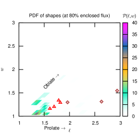
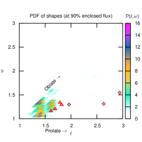
Figure 9: Same as 8, but for 80% and 90% enclosed flux.

3.3 Comparison with previous results

We compare our results with the results obtained by Limousin et al. (2013) and Chiu et al. (2018). Limousin et al. (2013) used triaxial model fitting to obtain the 3-D shape of 4 strong lensing clusters by combining X-ray, SZ and lensing data. Chiu et al. (2018) obtained the shapes of galaxy clusters using strong and weak lensing data. For most of the galaxy clusters, Chiu et al. (2018) are only able to constrain one of the axes ratios and provide only lower limits on the second axes ratio when they do not use any shape priors from simulations. They have given their results in the form of $T/L$ and $W/L$, which we convert to $\ell$ and $w$ for comparison, and tabulate the results in Table 4. We also show the axes ratios obtained in Limousin et al. (2013) and Chiu et al. (2018) along with our best-fitting PDFs in the $\ell-w$ plane in Fig. 10 and 11. We should emphasize that the points corresponding to Limousin et al. (2013) and Chiu et al. (2018) results are the $\ell,w$ values for individual clusters whereas the two points corresponding to our work are the two points on the shape PDF, $P(\ell,w)$, of the 89 Chandra clusters with the numbers referring to the relative probability amplitude of these points, $a_{i}$. Also our points refer to the shapes at different distances from the centre for which we use the fraction of X-ray flux enclosed by an isocontour on the X-ray surface brightness maps of the clusters. The earlier works obtain a single average shape for the cluster. Our results show that the shape of the halo is different as we move from the inner regions to the outskirts of the cluster.

In the innermost part of the cluster ($25\%$ enclosed flux), we find that the cluster shapes are predominantly prolate. There is preference towards oblateness as we move to the outskirts. The points from Limousin et al. (2013) are clustered together and are in rough agreement with our results. The points from Chiu et al. (2018) are more spread out and lean towards prolate shapes. However, we note that the Chiu et al. (2018) are measuring the shapes of dark matter halos while we are measuring the shape of the baryons. Taken together, these results may point towards a difference in shape of baryons and dark matter, however we need more data to make any definite conclusion.

Cluster	$\ell$	$w$	$\mathcal{T}$	Reference
Abell 1835	1.69	1.20	0.76 (prolate)	L2013
Abell 383	1.82	1.29	0.71 (prolate)
Abell 1689	1.79	1.34	0.64 (triaxial)
MACS 1423	1.61	1.16	0.78 (prolate)
Abell 209	1.96	1.30	0.76 (prolate)	C2018
MACS J0329-0211	2.94	1.55	0.82 (prolate)
RX J1347-1145	2.63	1.31	0.88 (prolate)

Table 4: List of galaxy clusters for which shapes have been obtained by fitting cluster models to multiple data-sets (Reference L2013: Limousin et al. (2013), Reference C2018: Chiu et al. (2018))

.

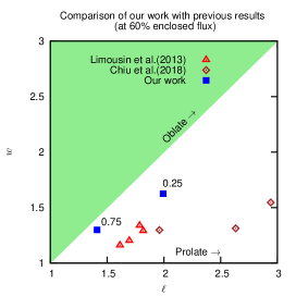
Figure 10: Comparison of the results obtained by us with the results of Limousin et al. (2013) and Chiu et al. (2018) in the $(\ell,w)$ plane. The blue square points obtained in this work are the approximation for the shape PDF, $P(\ell,w)$, of $87-89$ Chandra clusters with the numbers next to them the relative probability amplitude of the corresponding shape. The triangles and diamonds on the other hand are the axes ratios of individual clusters from previous works. The shaded light-green region is excluded by definition of $\ell,w$.

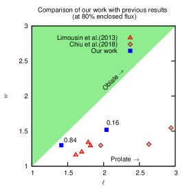
Figure 11: Same as 10, but for 80% and 90% enclosed flux. Analysis for these two cases has been performed with $78-81$ clusters.

4 Conclusions

We have presented a powerful new method to infer the PDF of shapes, $P(\ell,w)$, using only 2-D images of clusters of galaxies. To illustrate our method we have used X-ray images from publicly available Chandra data. Our method can also be applied to optical as well as SZ data. The main requirement for our method is a large sample of images, since we directly infer the PDF of shapes of the whole population rather than the shapes of individual clusters. We have also shown that our method is relatively insensitive to the density and temperature profiles of the clusters and thus does not require detailed 3-D modelling.

We find general consistency with the existing results of Limousin et al. (2013), who use data sensitive to baryons, such as X-rays and SZ effect, given the small statistical samples but differs significantly from the analysis of Chiu et al. (2018) who use only lensing data and are therefore sensitive to dark matter distribution. Our main results are that the shape of X-ray emitting gas is prolate for the innermost parts of the cluster, but shows a preference towards oblateness in the outer parts. The shapes of the haloes in dark matter simulations show preference towards prolateness in the inner parts(Frenk et al., 1988b; Dubinski & Carlberg, 1991; Warren et al., 1992; Bailin & Steinmetz, 2005; Bett et al., 2007), which is consistent with our results in the innermost parts. In these simulations, the haloes are found to be more oblate in outer parts, though prolateness is still predominant, except for Dubinski & Carlberg (1991) who find no preference towards prolate or oblate shape in the outskirts. Thus, our results in the outer parts are in contrast with the halo shapes found in dark matter simulations. However, it should again be noted that these simulation results are for the shapes of dark matter haloes, while we are measuring the shape of baryons.

We expect that the future X-ray and SZ surveys to detect hundreds of thousands of galaxy clusters (Merloni & German eROSITA Consortium, 2012; K. N. Abazajian et al., 2016). In order to apply our method, we will need these clusters to be imaged at high S/N by follow-up observations, similar to the Chandra cluster images in our selected sample. With large statistical samples, detailed statistical comparisons of observations with simulations, including evolution of shape with redshifts and dependence on mass, should become possible with our method.

Data availability

The data underlying this article are available in Chandra Data Archive (Chaser) at https://cda.harvard.edu/chaser/. The datasets used in this article were derived from the catalogue of Chandra clusters compiled by Eric Tittley and available at https://www.roe.ac.uk/~ert/ChandraClusters/. The list of clusters used in this article is given in Appendix B.

Appendix A Error propagation from Chandra X-ray Data and robustness of filamentarity PDFs

We can test the robustness of our method to noise in X-ray data as well as intrinsic departures of the cluster shapes from perfect ellipsoids by propagating the errors in the ellipse parameters from the X-ray images to the filamentarity PDFs. The noise in X-ray data as well as non-linear cluster physics would result in making the isocontours irregular. The scatter of the isocontours around the best-fit ellipse and the resulting errors on the ellipse filamentarity, therefore, capture both the important sources of error. We will call the departure of an isocontour from a perfect ellipse (or scatter of the isocontour points around the best fit ellipse) as isocontour noise. We show below explicitly that, for our sample, these errors are negligible compared to the Poisson errors due to the limited sample size. This analysis justifies our approach of ignoring these errors in the main text. In future, as more and more clusters are imaged in X-rays, the Poisson errors may become comparable with the isocontour noise with increasing sample size, and it will be important to propagate these errors to final results. As we show below, this is quite straightforward to implement. Furthermore, we can use the errors in filamentarity, $F$, as an additional selection criteria to remove the most irregular clusters before performing the shape analysis.

For each cluster listed in Appendix B, we obtain the isocontour corresponding to a given X-ray count. We fit this isocontour with an ellipse as described in detail in section 3. The fitting procedure gives us the best-fitting values of semi-major axis, $a$, and semi-minor axis, $b$, of the resulting ellipse, along with the covariance matrix, $cov(a,b)$, associated with the fit. We find that the error on $a$ and $b$ is small, typically $1$-$2\%$ in most cases. In this section, we propagate the error on $a$ and $b$ to the PDF of filamentarity of Chandra clusters, ${{\mathcal{P}}}_{\rm obs}(F)$.

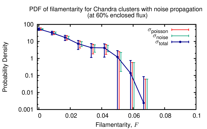
Figure 12: PDF of filamentarity, ${{\mathcal{P}}}_{\rm obs}(F)$, for Chandra X-ray clusters for 60% enclosed flux, obtained using 83 clusters after propagation of errors from isocontour noise and binned with a bin-width of $1/120$ in $F$. The rejection criterion leads to the rejection of 4 clusters from the original sample for which error in filamentarity ($\sigma_{F}$) is greater than the bin width. The 2 components of error, $\sigma_{poisson}$ and $\sigma_{noise}$, are shown alongside the total error, $\sigma_{total}$. Poisson error, which comes from the finite number of clusters, has the dominant contribution in the total error.

For a given cluster, we choose a random value $(a^{\prime},b^{\prime})$ from a 2D joint Gaussian probability distribution with mean ($a,b$) and covariance matrix $cov(a,b)$. We use $(a^{\prime},b^{\prime})$ to calculate the random sample of filamentarity $F^{\prime}$ for the corresponding cluster. We repeat this for every cluster and obtain the random sample of PDF of filamentarity, ${{\mathcal{P}}}_{\rm obs}(F^{\prime})$. We repeat the above steps 10000 times to generate 10000 samples ${{\mathcal{P}}}_{\rm obs}(F^{\prime})$ from the X-ray images of our cluster sample. In order to calculate the final PDF ${{\mathcal{P}}}_{\rm obs}(F)$, we take the mean and standard deviation of probability density values in each filamentarity bin across the 10000 PDFs. For a given bin, mean gives the probability density and standard deviation gives the propagated error from the isocontour noise. For each cluster, the standard deviation of the samples $F^{\prime}$ from the mean gives the error on the filamentarity of the corresponding cluster, $\sigma_{F}$. We can use a threshold on $\sigma_{F}$ to reject clusters with very irregular isocontours. For example, we would expect clusters which are not in virial equilibrium or are merging to have significant irregularities and departures from elliptical shapes. For the analysis in this appendix, we use the selection criteria that the error on the filamentarity should be less than our chosen bin width for $F$ and thus reject clusters with $\sigma_{F}>1/120$.

Thus, in addition to the Poisson error, we now have a new component, the isocontour noise, in the final PDF ${{\mathcal{P}}}_{\rm obs}(F)$. We calculate the total error in each bin of the final PDF as: $\sigma_{total}^{2}=\sigma_{\rm Poisson}^{2}+\sigma_{noise}^{2}$. The final PDF ${{\mathcal{P}}}_{\rm obs}(F)$ for $60\%$ enclosed flux is shown in Fig. 12, which shows that the Poisson error gives the dominant contribution in the total error. The additional $\sigma_{F}<1/120$ selection criteria results in rejection of 4 clusters from our original sample of 87 clusters for the $60\%$ flux case in Sec. 3. We show in Fig. 13 an example of 2 clusters which we have excluded using this criterion. We note that the results would not be affected significantly even if we do not use this additional rejection criterion and thus keep all the clusters for PDF calculation. This is demonstrated for ${{\mathcal{P}}}_{\rm obs}(F)$ of 60% enclosed flux in Fig. 14. The high $\sigma_{F}$ clusters would appear in different bins in different realizations/sample of $P(F)$ resulting in spreading out of the $P(F)$. In particular, the PDF spreads out to higher values of $F$ compared to Fig. 12. However, all the higher filamentarity values have large error bars and are consistent with zero, thereby keeping the final shape results unchanged. The $P(F)$ values not consistent with zero remain the same and are negligibly affected, whether we use the $\sigma_{F}$ rejection criterion or not.

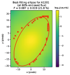
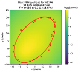
Figure 13: Smoothed X-ray surface brightness maps of Chandra clusters A1201 and A2146, along with the isocontour points and best-fitting ellipse, for 60% enclosed flux. These 2 clusters, among others, were not considered (rejected) for calculation of final PDF in this section, ${{\mathcal{P}}}_{\rm obs}(F)$, because the error in filamentarity is greater than the bin width of $1/120\sim 0.008$

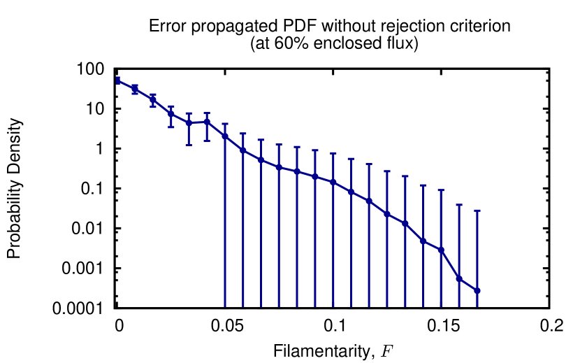
Figure 14: PDF of filamentarity, ${{\mathcal{P}}}_{\rm obs}(F)$, from Chandra X-ray clusters for 60% enclosed flux, obtained using 87 clusters after propagation of isocontour errors, without the rejection criterion. The error bars show total error. The longer tail compared to Fig. 12 is due to few clusters with higher isocontour noise, which leads to a spread in the filamentarity PDF. However, the filamentarity values in the additional bins in the long tail are all consistent with zero, while the non-zero values are the same as 12.

This analysis method has two advantages:

1. It allows us to obtain an estimate of the error on final PDF due to the errors on ellipse axes lengths $(a,b)$ coming from the isocontour noise. The isocontour noise (or irregular shapes of isocontours) maybe due to either noise in X-ray data (instrument noise or X-ray background) or intrinsic irregularities in the cluster (departure from virialization or merging clusters).

2. It gives us an additional tool to clean our sample and thus reject, for example, merging clusters. However, merging clusters would anyway have large errorbars and therefore lower statistical weight as they will spread out their contribution over many bins. Thus these clusters automatically would be suppressed and as long as there are not too many of them, they will not affect the results.

For our present analysis, however, we find that the Poisson errors dominate. In the future however, for a larger sample of clusters, Poisson errors may become sub-dominant. We have shown above, that in such a situation, we can propagate errors from X-ray images in a robust manner. Our method, when consistently propagating errors end-to-end, is particularly robust to contamination of the sample by un-virialized and merging clusters.

We use the final error-propagated filamentarity PDF (including rejection criterion) for Monte Carlo estimation of shape PDF, using the method outlined in section 3.2. The rejection criterion leads to the rejection of 8, 6, 4, 4, and 11 clusters for 25%, 40%, 60%, 80%, and 90% enclosed flux respectively. The results from this analysis are shown in Fig. 15 and 16. We find that these shape PDFs are consistent with the shape PDFs calculated in section 3.2. Thus, the results do not change significantly after the inclusion of propagated errors from isocontour noise and additional rejection criterion, thereby showing the robustness of our method.

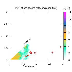
Figure 15: 2-D probability density of shapes in the ($\ell,w$) plane obtained using the Monte Carlo method, same as Fig. 8, but calculated using error propagated filamentarity PDF with rejection criterion. The shape PDF is close to the shape PDF in Fig. 8, thus showing that inclusion of propagated isocontour errors and rejection criterion does not change the results significantly.

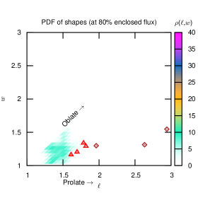
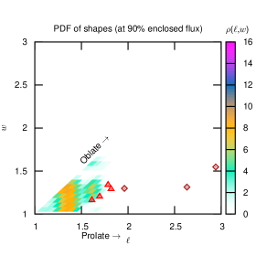
Figure 16: Same as 15, but for 80% and 90% enclosed flux

Appendix B List of galaxy clusters and Chandra data used in this work

Table 5: List of galaxy clusters and Chandra data used in this work.

S.No.	Object name	Observation ID
1	A3532	10745
2	3C348	1625
3	A3921	4973
4	4C55.16	1645
5	cl1212+2733	5767
6	cl0809+2811	5774
7	cl0318-0302	5775
8	cl0302-0423	5782
9	2PIGGz0.061 J0011.5-2850	5797
10	2PIGGz0.058 J2227.0-3041	5798
11	A3102	6951
12	cl1349+4918	9396
13	AWM4	9423
14	A0013	4945
15	A0068	3250
16	A0193	6931
17	A0209	3579
18	A0795	11734
19	A0586	19962
20	A0697	4217
21	A0744	6947
22	A0773	5006
23	A0801	11767
24	A0907	3185
25	A0963	903
26	A1068	1652
27	A1201	4216
28	A1204	2205
29	A1361	2200
30	A1413	1661
31	A1423	11724
32	A1446	4975
33	G125.70+53.85	15127
34	A1650	6356
35	A1664	7901

S.No.	Object name	Observation ID
36	A1763	3591
37	A1835	495
38	A3827	7920
39	A1914	542
40	A1930	A1930
41	A2009	10438
42	A2029	891
43	A2111	544
44	A2124	3238
45	A2142	5005
46	A2146	12246
47	A2151	4996
48	A2163	1653
49	A2187	9422
50	A2199	10803
51	A2204	499
52	A2218	553
53	A2219	14355
54	A2244	4179
55	A2259	3245
56	A2261	550
57	A2276	10411
58	A2294	3246
59	A2390	500
60	A2409	3247
61	A2426	12279
62	A2445	12249
63	A2485	10439
64	A2537	4962
65	A2550	2225
66	A2556	2226
67	A2589	6948
68	A2597	6934
69	A2626	3192
70	A2631	3248

S.No.	Object name	Observation ID
71	A2717	6974
72	A3112	2216
73	A3528s	8268
74	A3558	1646
75	A4059	5785
76	ACT J0616-5227	13127
77	AS1063	18611
78	AWM7	908
79	cl0956+4107	5759
80	cl1120+4318	5771
81	Cygnus A	360
82	ESO3060170-B	3188
83	MACSJ2311.5+0338	3288
84	PKS1404-257	1650
85	SERSIC 159-03	1668
86	A383	2321
87	A1689	7289
88	MACS-J0329.6-0211	3582
89	RXJ1347.5-1145	3592

References

- Altay et al. (2006) Altay G., Colberg J. M., Croft R. A. C., 2006, MNRAS, 370, 1422
- Aragón-Calvo et al. (2007) Aragón-Calvo M. A., van de Weygaert R., Jones B. J. T., van der Hulst J. M., 2007, ApJ, 655, L5
- Baddeley & Jensen (2004) Baddeley A., Jensen E., 2004, Stereology for Statisticians. Chapman & Hall/CRC Monographs on Statistics & Applied Probability, CRC Press, Boca Raton, doi:10.1201/9780203496817
- Bailin & Steinmetz (2005) Bailin J., Steinmetz M., 2005, The Astrophysical Journal, 627, 647
- Battaglia et al. (2012) Battaglia N., Bond J. R., Pfrommer C., Sievers J. L., 2012, ApJ, 758, 74
- Bett et al. (2007) Bett P., Eke V., Frenk C. S., Jenkins A., Helly J., Navarro J., 2007, Monthly Notices of the Royal Astronomical Society, 376, 215
- Bharadwaj et al. (2000) Bharadwaj S., Sahni V., Sathyaprakash B. S., Shandarin S. F., Yess C., 2000, The Astrophysical Journal, 528, 21
- Binggeli (1982) Binggeli B., 1982, Astronomy and Astrophysics, 107, 338
- Brunino et al. (2007) Brunino R., Trujillo I., Pearce F. R., Thomas P. A., 2007, MNRAS, 375, 184
- Buote & Canizares (1992) Buote D. A., Canizares C. R., 1992, in American Astronomical Society Meeting Abstracts #180. p. 823
- Buote & Canizares (1996) Buote D. A., Canizares C. R., 1996, Astrophysical Journal, 457, 565
- Carter & Metcalfe (1980) Carter D., Metcalfe N., 1980, Monthly Notices of the Royal Astronomical Society, 191, 325
- Chen et al. (2019) Chen H., Avestruz C., Kravtsov A. V., Lau E. T., Nagai D., 2019, MNRAS, 490, 2380
- Chiu et al. (2018) Chiu I.-N., Umetsu K., Sereno M., Ettori S., Meneghetti M., Merten J., Sayers J., Zitrin A., 2018, The Astrophysical Journal, 860, 126
- Clowe et al. (2004) Clowe D., De Lucia G., King L., 2004, MNRAS, 350, 1038
- Colless et al. (2001) Colless M., et al., 2001, Monthly Notices of the Royal Astronomical Society, 328, 1039
- Corless & King (2007) Corless V. L., King L. J., 2007, MNRAS, 380, 149
- Davis et al. (1985) Davis M., Efstathiou G., Frenk C. S., White S. D. M., 1985, ApJ, 292, 371
- Dubinski & Carlberg (1991) Dubinski J., Carlberg R. G., 1991, Astrophysical Journal, 378, 496
- Evans & Bridle (2009) Evans A. K. D., Bridle S., 2009, The Astrophysical Journal, 695, 1446
- Fabricant et al. (1984) Fabricant D., Rybicki G., Gorenstein P., 1984, Astrophysical Journal, 286, 186
- Frenk et al. (1988a) Frenk C. S., White S. D. M., Davis M., Efstathiou G., 1988a, ApJ, 327, 507
- Frenk et al. (1988b) Frenk C. S., White S. D. M., Davis M., Efstathiou G., 1988b, Astrophysical Journal, 327, 507
- Gavazzi (2005) Gavazzi R., 2005, A&A, 443, 793
- Geller & Huchra (1989) Geller M. J., Huchra J. P., 1989, Science, 246, 897
- Gott et al. (2005) Gott J. Richard I., Jurić M., Schlegel D., Hoyle F., Vogeley M., Tegmark M., Bahcall N., Brinkmann J., 2005, ApJ, 624, 463
- Green et al. (2019) Green S. B., Ntampaka M., Nagai D., Lovisari L., Dolag K., Eckert D., ZuHone J. A., 2019, ApJ, 884, 33
- Hadwiger (1957) Hadwiger H., 1957, Vorlesungen Über Inhalt, Oberfläche und Isoperimetrie. Berlin : Springer, doi:10.1007/978-3-642-94702-5
- Jing & Suto (2002) Jing Y. P., Suto Y., 2002, The Astrophysical Journal, 574, 538
- K. N. Abazajian et al. (2016) K. N. Abazajian et al. 2016, preprint, (arXiv:1610.02743)
- Kasun & Evrard (2005) Kasun S. F., Evrard A. E., 2005, The Astrophysical Journal, 629, 781
- Kawahara (2010) Kawahara H., 2010, The Astrophysical Journal, 719, 1926
- Klypin & Shandarin (1983) Klypin A. A., Shandarin S. F., 1983, MNRAS, 204, 891
- Lee & Suto (2004) Lee J., Suto Y., 2004, ApJ, 601, 599
- Lidstone (1932) Lidstone G. J., 1932, The Mathematical Gazette, 16
- Limousin et al. (2013) Limousin M., Morandi A., Sereno M., Meneghetti M., Ettori S., Bartelmann M., Verdugo T., 2013, Space Science Reviews, 177, 155
- Loken et al. (2002) Loken C., Norman M. L., Nelson E., Burns J., Bryan G. L., Motl P., 2002, ApJ, 579, 571
- Makarenko et al. (2015) Makarenko I., Fletcher A., Shukurov A., 2015, Monthly Notices of the Royal Astronomical Society: Letters, 447, L55
- Mantz et al. (2015) Mantz A. B., et al., 2015, MNRAS, 446, 2205
- Merloni & German eROSITA Consortium (2012) Merloni A., German eROSITA Consortium 2012, preprint, (arXiv:1209.3114)
- Navarro et al. (1996) Navarro J. F., Frenk C. S., White S. D. M., 1996, Astrophys. J., 462, 563
- Nelder & Mead (1965) Nelder J. A., Mead R., 1965, The Computer Journal, 7, 308
- Oguri et al. (2010) Oguri M., Takada M., Okabe N., Smith G. P., 2010, MNRAS, 405, 2215
- Oguri et al. (2012) Oguri M., Bayliss M. B., Dahle H., Sharon K., Gladders M. D., Natarajan P., Hennawi J. F., Koester B. P., 2012, Monthly Notices of the Royal Astronomical Society, 420, 3213
- Patiri et al. (2006) Patiri S. G., Cuesta A. J., Prada F., Betancort-Rijo J., Klypin A., 2006, ApJ, 652, L75
- Peter et al. (2013) Peter A. H. G., Rocha M., Bullock J. S., Kaplinghat M., 2013, MNRAS, 430, 105
- Piffaretti et al. (2003) Piffaretti R., Jetzer P., Schindler S., 2003, A&A, 398, 41
- Planck Collaboration et al. (2016) Planck Collaboration et al., 2016, A&A, 594, A24
- Rybicki & Lightman (1979) Rybicki G. B., Lightman A. P., 1979, Radiative processes in astrophysics. Wiley-Interscience, New York
- Samsing et al. (2012) Samsing J., Skielboe A., Hansen S. H., 2012, ApJ, 748, 21
- Sayers et al. (2011) Sayers J., Golwala S. R., Ameglio S., Pierpaoli E., 2011, The Astrophysical Journal, 728, 39
- Schmalzing et al. (1996) Schmalzing J., Kerscher M., Buchert T., 1996, in Bonometto S., Primack J. R., Provenzale A., eds, Dark Matter in the Universe, ProceedingsInternational School of Physics, Enrico Fermi , Course 132. IOS press, Amsterdam, p. 281 (arXiv:astro-ph/9508154)
- Shandarin & Zeldovich (1989) Shandarin S. F., Zeldovich Y. B., 1989, Reviews of Modern Physics, 61, 185
- Skielboe et al. (2012) Skielboe A., Wojtak R., Pedersen K., Rozo E., Rykoff E. S., 2012, The Astrophysical Journal, 758, L16
- Soucail et al. (1987) Soucail G., Fort B., Mellier Y., Picat J. P., 1987, Astronomy and Astrophysics, 172, L14
- Splinter et al. (1997) Splinter R. J., Melott A. L., Linn A. M., Buck C., Tinker J., 1997, ApJ, 479, 632
- Springel et al. (2005) Springel V., et al., 2005, Nature, 435, 629
- Sunyaev & Zeldovich (1972) Sunyaev R. A., Zeldovich Y. B., 1972, Comments on Astrophysics and Space Physics, 4, 173
- Vikhlinin et al. (2006) Vikhlinin A., Kravtsov A., Forman W., Jones C., Markevitch M., Murray S. S., Van Speybroeck L., 2006, ApJ, 640, 691
- Warren et al. (1992) Warren M. S., Quinn P. J., Salmon J. K., Zurek W. H., 1992, Astrophysical Journal, 399, 405
- Zeldovich (1970) Zeldovich Y. B., 1970, A&A, 5, 84
- Zeldovich & Sunyaev (1969) Zeldovich Y. B., Sunyaev R. A., 1969, Astrophysics and Space Science, 4, 301
- de Haan et al. (2016) de Haan T., et al., 2016, ApJ, 832, 95
- van Haarlem & van de Weygaert (1993) van Haarlem M., van de Weygaert R., 1993, ApJ, 418, 544