Properties of the Center of Gravity as an Algorithm for Position Measurements

Abstract

The center of gravity $x_{g}=\sum_{i}E_{i}x_{i}/\sum_{i}E_{i}$ as an algorithm for position measurements is carefully analyzed. Many mathematical consequences of discretization are extracted. The origin of the systematic error of the algorithm is shown to be connected to the absence of band limits in the Fourier Transform of the signal distributions, which, owing to the intrinsic properties of the measuring devices, must have a finite supports. However, special signal distributions exist among the finite support functions which are free from the discretized error. In the presence of crosstalk, it is proved that some crosstalk spreads are able to eliminate the discretization error for any shape (ideal detector). For all other cases, analytical expressions and prescriptions are given to correct the error and to efficiently simulate various experimental situations.

PACS: 07.05.Kf, 06.30.Bp, 42.30.Sy

Keywords: Center of Gravity, Centroiding, Position Measurements

1 Introduction 2019

The aim of this paper (published in Nuclear Instruments and Methods $\cdots$ A 485 2002 698-719) was the discussion and the calculation of the systematic error of the center of gravity (COG) (sometimes called weighted average or barycenter) as a positioning algorithm in one-dimensional geometry. The two-dimensional geometry is discussed in another paper. The arguments described here are relevant for recent developments.

The existence of the COG systematic error was known by a long time. In fact, one of our first work in high energy physics was just the elimination of the COG systematic error in the electron reconstruction of the Crystal Ball experiment. We never published the method, it used higher-order tensors and was very fast and precise. It was that experience that raised our interest in the problem, but only many years later we found the right mathematical tools (the Shannon sampling theorem [11]) to handle the problem. Our numerical simulations produced plots very similar to diffraction patterns in optics (as fig.2), but no waves are contained in the COG expressions. Where are the waves? The properties of the Fourier transform contained in the Shannon sampling theorem were the sought waves. This is the mathematical reason of our extensive (excessive?) use of Fourier transform and Fourier series. In any case the Fourier transforms are simple objects compared to the Bessel functions and the machinery required to extend the method to a sphere. We did it, but even the hard-disk considered it too complicated and decided to crash with a loss of all the work. We never did it again, but it is a possible task.

An important step was the introduction of the two-strip COG correction in 1983: the $\eta$-algorithm [16]. However, analytical expressions of this error (if any) was lacking, and a consistent elimination of it requires analytical form (or forms). The importance of the elimination of any systematic error in a fit is accurately discussed by Gauss in his paper of 1823. Here, Gauss stated that it is incorrect to handle the systematic errors as random errors after the availability of a "table" for those errors. It is natural to suppose that analytical expressions of systematic errors, as those of this paper, are equivalent (or better) than the tabular forms indicated by Gauss. Thus, applying the Gauss criterion, each paper that uses the COG positioning in a fit, without the proper correction of the systematic error, is incorrect at least from the date (2002) of this paper. It is evident that many papers were published with this type of error in the last years. This looks as a drop of the physics awareness that, without referring to the Gauss paper, knew very well the danger of the systematic errors.

Stimulated by these uncorrect papers, but independently from the Gauss paper, we proved the dangerous effects of the neglect of the COG corrections in ref.arXiv:1606.03051. That paper was a first version dedicated to the momentum reconstructions (the final version is published in INSTRUMENTS 2018 2 22 and arXiv:1806:07874). In one of the tests, the random noise was almost completely eliminated in the simulations. The distributions of the momentum reconstructions, based on positioning corrected by the COG systematic errors (eq.25 for example), showed a rapid convergence toward Dirac $\delta$-functions as expected. On the contrary, the momentum distributions based on the simple COG positioning remained invariant to the noise suppression: the detector quality (or better the signal-to-noise ration) becomes irrelevant in large extent. This result is in a perfect agreement with the Gauss warning about unpleasant effects given by systematic errors.

However, the study of the COG systematic error gave us a direct evidence of the necessity of a correction for each hit. A natural consequence was the necessity to construct a different probability distribution for each hit. Parts of the mathematical developments, discussed here, were used in the paper arXiv:1404:1968 (published by JINST 2014 9 P10006 ) for the construction of this type of probability distributions.

Among the by-products of the new probability distributions, an interesting effect was illustrated in INSTRUMENTS 2018 2 22: an approximate linear growth of the momentum resolution with the number $N$ of detecting layers. This growth is much faster than the $\sqrt{N}$ of the standard fit. To discuss better this linear growth, a simpler simulation with straight tracks was reported in ref. arXiv:1808.06708. Even here it is obtained a very large linear increase in the resolution of the fit parameters. To simplify, we will always speak of linear growth, even if small deviation from linearity are present. A Gaussian toy-model was introduced with a very simplified form of weights. This model is an easy illustration of the mechanism producing the linear growth. Among the simplified forms of weights, it was possible to connect the hit weights with the COG probabilities: the lucky-model.

The correct implementation of the lucky-model (as it was defined in arXiv:1808.06708), requires the elimination of the COG systematic errors or a their drastic reduction. The appropriate use of the analytical expressions for the COG can be an alternative to the more complicated $\eta$-algorithm. The lucky-model is a very economical tool for a drastic improvement of the fit resolution. The anomalies described here for the COG with a small number of strips must be accurately managed to use the lucky-model at large angles. Interesting enough, the inverse of effective weights of the lucky-model are strictly connected with eq.27 that describes the average signal distribution collected by a strip.

A line with the definition of the ideal detector is added at the end of subsection 6.6, it was forgotten in the writing of the paper. The subsection 6.6 describes a special kind of cross-talk that is able to suppress the COG systematic error for any form of signal distributions. The COG of this ideal detector is evidently compliant to the Gauss prescriptions. Detectors with floating strips tend to this ideal conditions, but the COG corrections are important even in this case.

We corrected few other printing errors, the formatting in a two columns style added few errors undetected at the time of the proof reading.

2 Introduction

The present generation of high-energy physics experiments shows a dramatic increase in the detector segmentation to capture the thinnest detail of the particle signals [1, 2]. These improvements must be completed together with improvements in the reconstruction algorithms. However, a reconstruction is always a pattern recognition, and the well-known ill-mathematical definition of any pattern recognition poses a serious problem to its generalization. Hence, almost always, the reconstruction algorithms are largely blended with ad hoc recipes to extract the best of the detector itself. Even if quite successful, their improvements are difficult to separate from the details of the detector, leaving few possibilities of exportation.

The aim of this work is to analytically treat the center of gravity (COG) algorithm, with particular attention to the effects of discretization. These results are mostly mathematical. For this reason, they are not bound by the above limitations and are applicable wherever the assumptions fit in the application. The use of the COG for position (and other) measurements is extremely widespread in scientific and practical applications, which are far too numerous to list here. Actually, only in rare cases can data analysis avoid calculating the COG of some signal distribution. We are primarily interested in high-energy physics applications, and our attention is focused on the topics we know best, as are our references.

At a superficial glance, widespread use of the algorithm is not unexpected: It actually looks very easy and easily justifiable. In fact the COG coincides with a symmetry point (line or plane) of the system. Hence, if the average image of the measured object on the measuring device has a symmetry property (point, line, or plane), the COG could give an estimation of its position. One drawback of this justification resides in the discretization that any automatic measuring device must perform on the image. Almost always, the discretization destroys any symmetry on the system, and the use of the COG introduces a systematic error in measurement which will be called even discretization error due to its origin in the discretization of the signal collection.

In high-resolution measurements, the presence of a systematic error in the algorithm is well known, and many empirical procedures have been developed to reduce its effect. Often, this fine-tuning requires lengthy and expensive Monte Carlo simulations or complex integration, with considerable probability of losing control of important details in the problem. More versatile and transparent methods are evidently of great help. No specific instrument will be considered, even if the declared polarization toward high-energy physics applications will be evident.

Here, we will limit ourselves to unidimensional geometry; the extension to bidimensional geometry is straightforward in some major cases. We will find classes of functions whose COGs are free of discretization error, but these results are probably of scarce use, since the selection of the signal distribution is rarely possible. An interesting consequence of these special functions is found on the crosstalk function. It turns out that if the crosstalk function is any of the above functions, the crosstalk saves the "energy" of the signal. Special crosstalk functions whose COGs are free of discretization error for any signal distribution will be defined.

We will determine analytical relations of continuous (almost everywhere) functions and their histograms. These relations are central to our study of the discretization effects. In its simplest form, the signals collected by a set of detectors are the histograms of the continuous signal distribution, and the bin size is equal to the size of the elementary detector (pixel, strips, crystal, etc.).

In Section 2, we introduce the problem with all the required definitions and examples. The systematic error is calculated with the easiest assumptions. We shall recall elements of signal theory, limiting ourselves to the strict necessities of the problem. All the derivations are based on standard properties of the Fourier Transforms (FT) and the Fourier Series (FS).

In Section 3, the conditions of the signal distributions which grant the absence of systematic error are discussed. Only exceptionally will the experimental signal distributions pertain to these classes and be free from error: For all other cases, equations will be given to relate true position with the COG.

A first analytical relation of a signal distribution with the histogram will be given in Section 4. This equation allows a direct simulation of the signal collection in the measuring device; it can easily be completed with noise models for the fine-tuning of empirical relations which go beyond the COG. We will define and apply a method for summing the first part of the double series encountered in the equations.

In Section 5, we extend this approach to the case of signal loss and crosstalk, defining their analytical aspects and properties. This allows a detailed treatment of a few reconstruction methods and experimental setups. The effects of crosstalk on signal collection and COG reconstruction are discussed in detail along with some of the unexpected properties of the crosstalk. Methods are developed to handle the suppression of the low-signal sensors. The discontinuities generated by these cutoffs are isolated. Reconstruction of position from a distribution of COG measurements is discussed and a few of its consequences and defects are pointed out.

Section 6 will address the study of the noise and signal fluctuations. A method for extracting fluctuations from a Monte Carlo simulation will be illustrated.

3 Sampling methods

3.1 Schematic properties of detectors

To accurately describe our problem, we shall consider the signal distribution of a high-energy photon showering in a homogeneous crystal detector with the geometry of the BGO calorimeter of the L3 experiment  [3] or the $\mathrm{PbWO}_{4}$ calorimeter of the CMS experiment [4]. Roughly speaking, these detectors consist of an array of truncated-pyramid shape crystals whose longest axis points toward the interaction center (if we neglect the small off-center distortion needed to reduce the energy loss at the crystal borders). Photons coming from the interaction point produce showers in an almost homogeneous medium, and their average has an axially symmetric shape whose symmetry axis coincides with the photon direction. The light collection projects the shower on a plane orthogonal to the photon direction and the symmetry point of the average distribution is the impact position of the photon. The readout system generates a set of numbers which in well-designed calorimeters are proportional to the energy released by the photon shower in each crystal [5]. Each detecting element can be approximated to a square pixel identical to all the others, and arranged in a regular flat orthogonal array. This bidimensional distribution can often be explored as two orthogonal unidimensional distributions due to the linearity of COG in the energy distribution. It is evident that this schematization is useless in a complex geometry such as that of the Crystal Ball detector [5].

An almost perfect unidimensional system is given by silicon micro strip detectors in a tracker system [6, 7]. Here, a particle traversing the detector distributes signals on a few contiguous, very long (infinite for our needs) parallel strips. The three-dimensional initial ionization has an average symmetry axis directed along the path of the incoming particle. The detector geometry allows the retrieval of discrete information on a unidimensional signal distribution $\psi(x)$. Here, and in the following, x is a reference axis on the detector plane, perpendicular to the strip direction, with its origin in the middle of a strip. For particle directions orthogonal to the strip plane, the point of symmetry of the average on $\psi(x)$ is the position of the impact point.

3.2 Average signal distribution

By $\varphi(x)$, we will indicate the average signal distribution for the impact point $\varepsilon=0$. The function $\varphi(x)$ and its discrete reduction performed by the readout system will be the focus of the present investigation. Let us first consider the properties of $\varphi(x)$ which will be required in the following:

a) $\varphi(x)$ is real and symmetric around zero $\varphi(x)=\varphi(-x)$

b) $\varphi(x)$ is continuous almost everywhere and has a continuous and derivable FT

c) $\varphi(x-\varepsilon)$ is the signal distribution in a homogeneous medium when the impact point is $\varepsilon$.

We will call $\varepsilon$ the impact point, in the jargon of high-energy physics. In general, $\varepsilon$ is the position of the symmetry point of the average signal distribution for any kind of signal source. Our results are valid even for asymmetrical $\varphi(x)$. In this case, $\varepsilon$ is the position of the COG of $\varphi(x)$, but in the equations we will explicitly use the symmetry of $\varphi(x)$.

To simplify the notation, we normalize $\varphi(x)$ as $\int_{-\infty}^{+\infty}\varphi(x)dx=1$. In addition, in some derivations, we will need $\varphi(x)$ to be positive with a single maximum.

From points a) and b), it is clear that $x_{g}$ defined as $x_{g}=\int_{-\infty}^{+\infty}x\varphi(x)dx$ to be the COG of $\varphi(x)$ is zero. The impact point $x_{i}=\varepsilon$, yields the identity $x_{g}=\varepsilon$. All the values of $x_{g}$ are independent of the details of signal distribution and, at this level, the method is a perfect position measuring device. However, $\varphi(x)$ is not accessible by the experiments nor it is normalized. The readout system performs a discrete reduction that drastically modifies the method’s measuring effectiveness. In its simplest form, the discrete reduction amounts to a set of finite disjointed integrations on the signal distribution, spoiling it from any simple connection to $\varphi(x)$ and to $\varepsilon$. So, the readout data consist of a set of numbers (very few indeed) $\alpha_{n}(\varepsilon)$ defined by:

$$\alpha_{n}(\varepsilon)=\int_{n\tau-\tau/2}^{n\tau+\tau/2}\varphi(x-\varepsilon)dx$$

where $\tau$ is the distance of the strip axis (or the axis of any other detector array) and $\alpha_{n}(\varepsilon)$ is the signal collected by the strip $n$ (or the sum of the signals collected by a line of detectors orthogonal to the x-axis). Now, the COG is defined by $x_{g}=\sum_{n}\alpha_{n}(\varepsilon)\tau n/\sum_{n}\alpha_{n}(\varepsilon)$. The reference system has its zero on the middle of the detector with the maximum signal, and we can limit ourselves to exploring the region with $|\varepsilon|\leq 1/2$. Excluding the case of $\tau\rightarrow 0$ and $n\rightarrow\infty$, it is evident that the discretized $x_{g}$ differs from $\varepsilon$ almost everywhere.

3.3 Sampling

To obtain explicit relations, we shall use a few elements of signal theory. As is often done in signal theory, we can rescale all the lengths to have $\tau=1$ without loss of generality, but the practical use of the equations can entail some ambiguities which might well be avoided. The tradeoff is an additional symbol to handle, but, at the same time, the equations retain the proper dimensions. First, we have to define the functions:

$$f(x)=\int_{-\infty}^{+\infty}\Pi(\frac{x-x^{\prime}}{\tau})\varphi(x^{\prime})\mathrm{d}x^{\prime}\$$

$$f_{\varepsilon}(x)=\int_{-\infty}^{+\infty}\Pi(\frac{x-x^{\prime}}{\tau})\varphi(x^{\prime}-\varepsilon)\mathrm{d}x^{\prime},$$ (1)

where $\Pi(t)$ is the interval function $\Pi(t)=1$ for $|t|<1/2$ and $\Pi(t)=0$ elsewhere, and wherever needed, $\Pi(\pm 1/2)=1/2$. This is one of the simplest linear transforms. More complex cases will be explored in the following sections. Due to the symmetry of $\Pi(t)$ and $\varphi(x)$, function $f_{\varepsilon}(x)$ is symmetric with respect to $x=\varepsilon$ . The properties of convolutions [8] state that $f_{\varepsilon}(x)$ is equal to $f(x-\varepsilon)$ and the COG of $f_{\varepsilon}(x)$ is the sum of the COGs of $\Pi(x)$ and $\varphi(x-\varepsilon)$. The first is zero, the second is $\varepsilon$ , and the COG of $f_{\varepsilon}(x)$ is that of $\varphi(x-\varepsilon)$. Now,

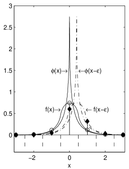
Figure 1: $\phi(x)$ is the signal distribution with zero impact point, f(x) is its convolution with an interval function. The dots are the signals collected by the detectors centered at x=-3,-2,-1,0,1,2,3 and are samples of f(x). $\phi(x-\varepsilon)$, f$(x-\varepsilon)$ and the diamonds are as above for an impact point $\varepsilon$. Dashed lines are the borders of the detectors.

the $\alpha_{n}(\varepsilon)$ values are given by the sampling of $f_{\varepsilon}(x)$ at each $n\tau$ $(n=0,\pm 1,\pm 2,....)$ and they are the signals collected by the detectors whose axes is located at points $x=n\tau$ as shown in Figure 1. The set $\{\alpha_{n}(\varepsilon)\}$ can be formally expressed as a function of $x$ with a series of Dirac $\delta$-functions:

$$s_{\varepsilon}(x)=\sum^{+\infty}_{n=-\infty}\alpha_{n}(\varepsilon)\delta(x-n\tau)$$ (2)

$$s_{\varepsilon}(x)=f(x-\varepsilon)\sum^{+\infty}_{n=-\infty}\delta(x-n\tau).$$ (2’)

Defining $S_{\varepsilon}(\omega))$ the FT of $s_{\varepsilon}(x)$, $x_{g}$ is given by the relation [8]:

$$x_{g}=i\frac{1}{S_{\varepsilon}(0)}\frac{dS_{\varepsilon}(\omega)}{d\omega}\mid_{\omega=0}$$ (3)

and, defining $F_{\varepsilon}(\omega)$ as the FT of $f_{\varepsilon}(x)$, the Poisson identity [9] relates $S_{\varepsilon}(\omega)$ with $F_{\varepsilon}(\omega)$:

$$S_{\varepsilon}(\omega)=\tau^{-1}\sum_{k=-\infty}^{+\infty}F_{\varepsilon}(\omega-2\pi k/\tau).$$ (4)

A sketchy justification of the Poisson identity can be given with the observation that Eq. (2’) is the product of two functions, but one is periodic with period $\tau$. Its FT is a sum of Dirac $\delta$-functions with arguments $(\omega-2\pi k/\tau)$, and the convolution of $F_{\varepsilon}(\omega)$ with this sum of Dirac $\delta$-functions, assumes the form of Eq. (4). According to the convolution theorem and the shift property of FT, $F_{\varepsilon}(\omega)$ is equal to:

$$F_{\varepsilon}(\omega)=2\frac{\sin(\omega\tau/2)}{\omega}\Phi(\omega)e^{-i\varepsilon\omega},$$ (5)

where the first term is the FT of $\Pi(x/\tau)$, and $\Phi(\omega)$ is the FT of $\varphi(x)$. The function $\Phi(\omega)$ is real and symmetric, with $\Phi(0)=1$ for the normalization, and its first derivative is zero at $\omega=0$. The absence of loss in the signal collection fixes the normalization of $s_{\varepsilon}(x)$ as that of $\varphi(x)$; actually, it is $F_{\varepsilon}(-2\pi k/\tau)=0$ for $k\neq 0$ and $F_{\varepsilon}(0)=\tau$ giving $S_{\varepsilon}(0)=1$ in Eq. (4). From Eqs. (3)-(5), and with the properties of $\Phi(\omega)$, the explicit form of $x_{g}(\varepsilon)$ turns out to be:

$$x_{g}=\varepsilon+\frac{\tau}{\pi}\sum_{k=1}^{\infty}\frac{(-1)^{k}}{k}\sin(2\pi k\varepsilon/\tau)\Phi(2\pi k/\tau).$$ (6)

The first term of Eq. (6) is the COG of $f_{\varepsilon}(x)$ or of $\varphi(x-\varepsilon)$. It is independent of the shape and the sampling period and is thus the perfect measuring device we mentioned. The other terms are the systematic error of the algorithm due to the sampling of the $f_{\varepsilon}(x)$ at $\tau$ intervals. Their $\varepsilon$-dependence has the form of an FS of an odd function of with amplitudes $(-1)^{k}\Phi(2\pi k/\tau)/k$ and period $\tau$ as conjectured in [10]. This periodicity is due to the form of the sampling function in Eq. (2) which is periodic as well. Physically, this amounts to considering an infinite row of identical detectors. In Section 5, we will abandon this condition to handle more realistic cases. It is evident in Eq.(6) that $x_{g}=\varepsilon$ for $\varepsilon=0$ and $\varepsilon=\tau/2$ and for all other integer and semi-integer values of $\tau$, that is a consequence of the symmetry of our detector setup which survives in these special points.

If $\varphi(x)$ converges to a Dirac $\delta$-function, $x_{g}$ reaches the maximum error, as expected. In this case, where $\Phi(2\pi k/\tau)$ converges to one, the series in Eq. (6) is the Euler $sine$ series [8], and $x_{g}$ becomes identical to zero for $|\varepsilon|<\tau/2$ and $x_{g}=\varepsilon$ for $|\varepsilon|=\tau/2$.

4 Special Shapes

4.1 The absence of discretization error

Let us now examine the error of $x_{g}$ as expressed by Eq.(6) in greater detail. The FS form of $x_{g}-\varepsilon$ allows the analytic calculation of the mean square value on a period $|\varepsilon|\leq\tau/2$ with the Parseval identity:

$$\Delta^{2}=\frac{1}{\tau}\int_{-\tau/2}^{+\tau/2}(x_{g}-\varepsilon)^{2}=\frac{\tau^{2}}{2\pi^{2}}\sum_{k=1}^{\infty}\Phi^{2}(\frac{2\pi k}{\tau})k^{-2}.$$ (7)

This equation sheds some light on the origin of error $\Delta$ and defines the conditions on $\varphi(x)$ which give $x_{g}=\varepsilon$ . It is evident that $\Delta$ is equal to zero if $\Phi(2\pi k/\tau)=0$ for $k>0$. Hence, excluding some very special cases discussed later on, the class of band-limited functions, with $\Phi(\omega)=0$ for $|\omega|\geq 2\pi/\tau$, has always $x_{g}$ equal to $\varepsilon$ . Part of this result is not wholly unexpected. Due to the Wittaker Kotel’nikov Shannon (WKS) sampling theorem [9, 11], the subclass of the band-limited functions, with $\Phi(\omega)=0$ for $|\omega|\geq\pi/\tau$, has the property that $f_{\epsilon}(x)$ can be exactly reconstructed from its sampled values $\alpha_{n}(\varepsilon)$ ${n=0,\pm 1,\pm 2,...}$, as can its COG. But the condition for $\Delta=0$ in Eq. (7) is broader than that of the WKS theorem. Here, the absence of overlap of the shifted functions $\Phi(-2k\pi/\tau)$ $(k=\pm 1,\pm 2,..)$ with $\Phi(\omega)$ at $\omega=0$ suffices, and $x_{g}=\varepsilon$ remains true, even when the sampling interval must be $\tau/2$ for the WKS theorem. These properties of $\Delta$ remain valid even if $\varphi(x)$ is asymmetric. In a broader sense, the error $\Delta$ originates from an aliasing effect at $\omega=0$ due to the sampling of $f_{\varepsilon}(x)$ at an overly large interval.

Apart from the mathematical interest of a theorem regarding the set of sampled functions with $x_{g}$ equal to $\varepsilon$ , the previous condition is of little practical use for our problem. Other theorems [9] prove that band-limited functions $\varphi(x)$ cannot be zero in any finite segment of the $x$-axis, i.e., $\varphi(x)$ and $f_{\varepsilon}(x)$ would be different from zero almost everywhere in x. This property is very far from standard experimental situations where $\varphi(x)$ is different from zero only in a narrow region of the $x$-axis covering few $\tau$’s ($3\sim 5$ at best). Beyond this region, $\varphi(x)$ rapidly plunges below the readout noise and must be put equal to zero. Hence, the necessity of keeping the signal well above the readout noise to increase detection probability works adversely to the sensitivity of the subpixel position measurement. The extreme case of $\varphi(x)$ converging to a Dirac $\delta$-function is a clear example. This shape maximizes the detection probability, but leaves its subpixel position completely undermined, and the mean square error gets its maximum $\Delta^{2}=\tau^{2}/12$. Simulations will show that practical situations are intermediate between the full indeterminateness of the Dirac $\delta$-function and a good reconstruction.

Equation (7) allows the selection of a set of special shapes and sizes which have $x_{g}=\varepsilon$ , even if these are not band-limited. More simply, we have to find functions that have $\Phi(\omega)=0$ for $\omega=2k\pi/\tau$ $(k=\pm 1,\pm 2,\pm 3..)$ and $\Phi(0)=1$. It should be pointed out that this distribution of zeros pertains to the function $\sin(\omega\tau/2)/(\omega)$ and to any of its integer powers and products with functions regular at $\omega=2k\pi/\tau$. The simplest functions whose FTs have the above property are the rectangular functions whose sizes are integer multiples of $\tau$. More complex functions are the convolutions of identical rectangular functions. These have special sizes with $x_{g}=\varepsilon$. For example, triangular functions (convolutions of two identical rectangular functions) with sizes that are even multiples of $\tau$ have $x_{g}=\varepsilon$ . Evidently, this is true for any linear combination of these special functions and for any convolution with functions that have FTs regular at $\omega=2k\pi/\tau$. This class of functions is very large, but the minimum size allowed is $\tau$ and the convolutions with the minimum-size rectangular function have sizes $\tau+D$ (where D is the size of the convolved function).

An application of these considerations is possible when $\varphi(x)$ can be expressed as a convolution with a rectangular function. Now, if the size of the detector coincides with that of the rectangular function, the position reconstruction with the COG algorithm does not require corrections. In all the other cases, knowledge of $\varphi(x)$ is required to extract $\varepsilon$ given $x_{g}$ as in Eq. (6).

4.2 Examples

From now on, we shall consider only the class of finite support functions, i.e., $\varphi(x)\neq 0$ for $|x|<D/2$. Equation (6) has the form of an infinite series, but its terms rapidly decrease, at least as $k^{-2}$, as in the worst case of a rectangular distribution, and the sum can be cut off after a reasonable number of terms. In the simulations of Eqs. (6) and (7), we will explore only four shapes: a rectangle, a triangle, a cylinder, and a cone. The first two depend solely on $x$; the second two depend on $x$ and $y$ and must be integrated on $y$ for our geometry. The rectangle and triangle have easy FTs, while for the y-integrated cylinder and cone, we obtain the FTs integrating with the $J_{0}(\omega r)$ Bessel function (Hankel transform). These simple shapes alone are unable to cover many realistic conditions. To maximize detection efficiency, a large fraction of the signal $(70\sim 80\%)$ is often concentrated on a single pixel.

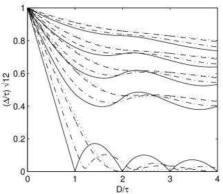
Figure 2: Plots of $(\Delta/\tau)\surd 12$ versus D/$\tau$ for the linear combination of two shapes with D’/D=1/20, $\beta$=0,2,4,8 and four shapes: solid lines for rectangles, dot-dash lines for cylinders, dashed lines for triangles, and dotted lines for cones.

To gain some information on the COG error of this kind of signal distributions, we will simulate them with a linear combination of two identical functions differing in size D and D’:

$$\varphi(x)=[\varphi_{D}(x)+\beta\varphi_{D^{\prime}}(x)]/(1+\beta)$$ (8)

The variations in parameter $\beta$ , size D, and ratio D’/D allow a large increase in the shapes explored. Figure 2) shows $(\Delta/\tau)\surd 12$, versus $D/\tau$, for D’/D=1/20, $\beta=0,2,4,8$ and the four shapes. Increasing $\beta$ , i.e., increasing the signal released in the central pixel, $\Delta$ increases rapidly reaching values almost shape-independent. For $\beta=0$ (the lowest plots), the sizes for which the rectangular and triangular shapes have $\Delta=0$ are evident. The similarities of the cylinder and the cone with the rectangle and triangle are remarkable.

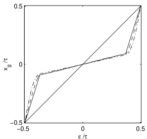
Figure 3: $x_{g}$ versus $\varepsilon$ for D=1.8, D’/D=1/7, $\beta$=3.5, $\tau$=1 and the graphical conventions as in Figure 1.

Figure 3) shows the plot of Eq.(6) for linear combinations whose $\alpha_{n}(\varepsilon)$ distributions are roughly similar to those generated on the y-side of the PAMELA silicon tracker [7] by a minimum ionizing particle. In principle, this plot allows the extraction of $\varepsilon$ given $x_{g}$, or verification of the optimization of an algorithm.

5 Histograms

5.1 Finite support functions

To simulate the reconstruction, it is useful to define a general aspect of the finite support functions $\varphi(x)$, i.e., $\varphi(x)=0$ for $|x|\leq D/2$. The function $\varphi(x)$ can be expressed as the product of a periodic function with the interval function $\Pi(x/D)$ which selects a single period. The periodic part coincides with $\varphi(x)$ where $\varphi(x)\neq 0$ and can be expressed as FS. The symmetry simplifies the form $\varphi(x)$ becoming:

$$\varphi(x)=D^{-1}\Pi(x/D)[\Phi(0)+2\sum_{n=1}^{\infty}\Phi(\gamma_{n})\cos(\gamma_{n}x)].$$ (9)

The parameters $\Phi(\gamma_{n})$ are the values of $\Phi(\omega)$, the FT of $\varphi(x)$, calculated at the FS-frequencies $\gamma_{n}=2\pi n/D$, and the dual form of the WKS theorem express the form of $\Phi(\omega)$ with the parameters $\Phi(\gamma_{n})$. The normalization fixes $\Phi(0)=1$ for any D, so $\varphi(x)$ must scale on D as $\varphi(x)\rightarrow\varphi(x/D)D^{-1}$ and the parameters (form factors) $\Phi(\gamma_{n})$ turn out to be $D$-independent. This property is very convenient for our use of a linear combination of identical functions with different support $D$ as in Eq. (8). Here, only a set of $\Phi(\gamma_{n})$ must be calculated, and the cutoff on the high frequencies of $\Phi(\omega)$ is identical for the two (or more) functions which form $\varphi(x)$.

For signal distributions scaling with a length $L_{M}$ typical of the material, Eq.(9) has another interesting property: $D$ scales with $L_{M}$, and the set $\Phi(\gamma_{n})$ is independent of the material, and can be defined once and for all. An example of this is the average photon shower and its lateral scaling with the Molier radius [5].

5.2 Histograms

Using Eqs.(1) and (9), the function $f(x)$ can be calculated explicitly, and for $D>\tau$ becomes:

$$f(x)= \frac{1}{D}\Big{\{}\tau+g_{+}(x)[x+\frac{D-\tau}{2}]+g_{-}(x)[x-\frac{D+\tau}{2}]\Big{\}}+$$

$$\sum_{n=1}^{\infty}\frac{1}{\pi n}\Big{\{}\sin[\gamma_{n}(x+\frac{\tau}{2})][1-g_{-}(x)]-\sin[\gamma_{n}(x-\frac{\tau}{2})][1-g_{+}(x)]\Big{\}}\Phi(\gamma_{n})$$ (10)

where $g_{\pm}(x)=\Pi((2x\pm D)/2\tau)$ and $x$ is limited by $-(D+\tau)/2<x<(D+\tau)/2$. Outside this interval, $f(x)$ is zero. For $D\leq\tau$, $f(x)$ equals Eq. (10), excluding the region $(-\tau+D)/2<x<(\tau-D)/2$ where $f(x)=1$. In Eq. (10), functions $g_{\pm}(x)$ are introduced to write in compact form the changes due to different integration limits. The tradeoff for compactness is difficulty for the differentiating.

The sampling of $f(x)$ at points $x_{m}=m\tau-\varepsilon$ (for $m=\pm 1,\pm 2,..$) generates the set $\{\alpha_{m}(\varepsilon)\}$. With a realistic noise model, Eq. (10) allows the simulation of the experimental data given the form factors $\Phi(\gamma_{n})$, or it allows the extraction of the form factors $\Phi(\gamma_{n})$, given a value of $D$, from a distribution of experimental data (as done in a slightly different way in  [12]). For construction, the samples of $f(x)$ at points $x_{m}=m\tau-\varepsilon$ generate the histogram of $\varphi(x)$ with bin-size $\tau$. The generalization of Eq.(10) to an asymmetric function $\varphi(x)$ is simple. Quite often, the fit to histogram is done directly with $\varphi(x)$; assuming its value proportional to the value at the center of each histogram’s bin, it is evident that $f(x)$ (not $\tau\varphi(x)$) has this property. This inconsistency almost always disappears as the bin-size goes to zero for regular functions.

Improved centroid algorithms can be obtained by fitting $f(x)$ with a few parameter functions and extracting $f(x-\varepsilon)$ and $\varepsilon$ from the experimental data as done in [10] in a special case. These algorithms are often called "nonlinear COGs" [13], but their extraction from a set of predefined solutions as experimented in [13] looks very improbable. Matching case by case is probably the only way to proceed.

5.3 Sum of the series

In Eq. (10), the infinite series have terms decreasing as fast as $n^{-(|m|+1)}$ if $m$ is the degree of continuity of $\varphi(x)$, Hence, not too many terms are required to arrive at a significant result. Equations (6) and (7) require $\Phi(2n\pi/\tau)$ values differing from the form factors $\Phi(\gamma_{n})$. The connection between these two sets is given by the dual formulation of the WKS theorem which states that the FT of Eq. (9), $\Phi(\omega)$, is given by:

$$\Phi(\omega)=\sum_{n=-\infty}^{+\infty}\Phi(\gamma_{n})\frac{\sin(\omega D/2-n\pi)}{(\omega D/2-n\pi)}.$$ (11)

This procedure can be quite cumbersome in cases such as axially symmetric bidimensional shapes which often have complicated FTs. In addition, for signal distributions that scale with a length typical of the material, the set of values $\{\Phi(\gamma_{n})\}$ is material independent, and hence it is important to express the COG systematic error by those values. For this task, we found a way of summing the $k$-dependence of Eq. (6) for any $\varepsilon$ and $D$. With the general form of $\Phi(\omega)$ given by the WKS theorem, the $k$-series for $x_{g}$ becomes:

$$x_{g}=\varepsilon-\frac{\tau}{4\pi}{\sum_{k=-\infty}^{+\infty}}_{k\neq 0}\frac{(-1)^{k}}{k}\sum_{n=-\infty}^{+\infty}\Phi(\gamma_{n})\frac{(-1)^{n}\big{[}e^{i2k\pi(\varepsilon+D/2)/\tau}-e^{i2k\pi(\varepsilon-D/2)/\tau}\big{]}}{(kD\pi/\tau-n\pi)}.$$ (12)

Exchanging the order of the sums, we can recast the sum on $k$ as an integration along a closed line [14] multiplied by an integration function $[\sin(\pi z)]^{-1}$ that has poles for integer $z$-values:

$$x_{g}=\varepsilon-\frac{\tau}{4\pi}\sum_{n=-\infty}^{+\infty}(-1)^{n}\Phi(\gamma_{n})\oint_{C_{1}}dz\frac{1}{z\sin(\pi z)}\frac{\big{[}e^{i2k\pi(\varepsilon+D/2)/\tau}-e^{i2k\pi(\varepsilon-D/2)/\tau}\big{]}}{(\frac{\pi zD}{\tau}-n\pi)},$$

$C_{1}$ is a closed path which encircles all the poles of $[\sin(\pi z)]^{-1}$, but excludes the $z=0$ pole and all the poles of $\Phi(\omega)$. The coincidence of the $\Phi(\omega)$ poles with that of $[\sin(\pi z)]^{-1}$ can be avoided by adding a small imaginary part to the denominators of $\Phi(\omega)$ and keeping the limit at the end of the sum. Path $C_{1}$ can be deformed toward an infinite circle, and, if the integral goes to zero on this path, the sum of the residues at $z=0$ and at the poles of $\Phi(\omega)$ gives the sum of the series. The integral is zero on the infinite circle if $|(2\varepsilon\pm D)/2\tau|\leq 1/2$ i.e., in this case the exponents in the numerator of Eq.(12) are smaller or equal to that of the $[\sin(\pi z)]^{-1}$. This limitation on $\varepsilon$ and $D$, however, is too restrictive to render the summation useful. We need the sum for values of $\varepsilon$ and $D$ as large as they may be. To overcome this, we can observe that, in many cases, the WKS theorem could not be used for $\Phi(\omega)$, since a large set of candidates $\varphi(x)$ has a simple closed FT. For these functions, at the $\varepsilon$ value for which $|(2\varepsilon\pm D)/2\tau|=1/2$, the $k$-sum is regularly convergent. These limits simply indicate the point where a second strip starts to collect signals. Hence, with the sum being convergent, we can try to remove the limitations to the residue theorem. We can observe that the contribution to $x_{g}$ in Eq. (12) from the two exponents $\xi_{\pm}=(2\varepsilon\pm D)/2\tau$ is through periodic function with period one, and adding or subtracting an integer number to $\xi_{\pm}$ in the exponents leaves the sum of the series without variation. This allows the substitution of $\xi_{\pm}$ with $\xi_{\pm}+m_{\pm}$ in Eq. (12) where $m_{\pm}$ are integers that always give $|\xi_{\pm}+m_{\pm}|\leq 1/2$. Now the integral in Eq. (12’) can be calculated with the residue theorem for any value of $\varepsilon$ and $D$. To give a functional form to the previous transformation of $\xi_{\pm}$, it is convenient to use the function $\Theta(\xi_{\pm})=\xi_{\pm}-\mathrm{floor}(\xi_{\pm}+1/2)$. This is a sawtooth function, with $|\Theta(\xi_{\pm})|\leq 1/2$. Note that any other definition of a sawtooth function works identically. Our form is very convenient in computer usage, but it is not suited for derivation. The sum of the series in Eq. (12) becomes:

$$x_{g}=\varepsilon+\frac{\tau^{2}}{2D}\big{[}\Theta^{2}(\xi_{-})-\Theta^{2}(\xi_{+})\big{]}+\frac{\tau}{2\pi}\sum_{n=1}^{+\infty}\frac{(-1)^{n}\Phi(\gamma_{n})}{n\sin(\gamma_{n}\tau/2)}\big{\{}\cos[\gamma_{n}\tau\Theta(\xi_{+})]-\cos[\gamma_{n}\tau\Theta(\xi_{-})]\big{\}}$$ (13)

$$\xi_{\pm}=(2\varepsilon\pm D)/2\tau$$

$$\Theta(\xi_{\pm})=\xi_{\pm}-\mathrm{floor}(\xi_{\pm}-1/2)$$

Here $x_{g}$ is linear in the form factors $\Phi(\gamma_{n})$ and is suited for a best fit to extract $\varphi(x)$ from the measured function $x_{g}(\varepsilon)$. Equation (13) gives an explicit and simple form for a rectangular shape where all the $\Phi(\gamma_{n})$’s are zero. For an assembly of two rectangular functions, $x_{g}$ is:

$$x_{g}=\varepsilon+\frac{\tau^{2}}{2(1+\beta)}\Big{\{}\big{[}\Theta^{2}(\frac{2\varepsilon-D}{2\tau})-\Theta^{2}(\frac{2\varepsilon+D}{2\tau})\big{]}\frac{1}{D}+\big{[}\Theta^{2}(\frac{2\varepsilon-D^{\prime}}{2\tau})-\Theta^{2}(\frac{2\varepsilon+D^{\prime}}{2\tau})\big{]}\frac{\beta}{D^{\prime}}\Big{\}}.$$

An assembly of identical functions, scaled with D as in Eq.(8), has the same $\Phi(\gamma_{n})$ terms, and they factor out. We can see here a reason for $\varphi(x)$ in the form of Eq. (8), and how important the proper selection of the ranges D and D’ (or more) is. The number of $\Phi(\gamma_{n})$ to be used in Eq. (13) can be drastically reduced.

6 A more complex setup

6.1 Generalization of the spatial integrator

With few modifications, these approaches can be extended to a detector set that does not operate on the signal as a perfect spatial integrator. This is a frequent case: For example, the crystal detectors of an em calorimeter do not collect the light with constant efficiency over all their sizes. They have signal losses at their borders due to mechanical tolerances or to nonhomogeneous light absorption at the borders, with the effective efficiency modulated over the crystal.

In silicon strip detectors, the signal collection is even more complex. Some setups have unread strips which spread the signal by capacitive couplings among nearby strips as in the AMS [14] or PAMELA [7] trackers. To handle these situations, Eq. (1) must be generalized:

$$\mathrm{f}(x)=\int_{-\infty}^{+\infty}\mathrm{p}(x-x^{\prime},\tau_{1})\varphi(x^{\prime})dx^{\prime}$$ (14)

$$\mathrm{f}_{\varepsilon}(x)=\int_{-\infty}^{+\infty}\mathrm{p}(x-x^{\prime},\tau_{1})\varphi(x^{\prime}-\varepsilon)dx^{\prime}$$

Now $\mathrm{p}(x,\tau_{1})$ is a generic response function symmetric around zero with a finite range $\tau_{1}$ (the sampling distance is always $\tau$). For $\tau_{1}<\tau$, there is a definite signal loss; for $\tau_{1}>\tau$ there is a long range coupling (crosstalk) and the signal collected by a strip modifies the signal collected by the nearby strips. From Eq.(14), $\mathrm{p}(x,\tau_{1})$ is the response function of the detector to a Dirac $\delta$-signal. Due to its finite range and symmetry, the form of $\mathrm{p}(x,\tau_{1})$ resembles Eq. (9):

$$\mathrm{p}(x,\tau_{1})=\Pi(x/\tau_{1})[G_{0}+2\sum_{n=1}^{+\infty}G_{n}\cos(2\pi x/\tau_{1})].$$ (15)

Its FT is given by the WKS theorem:

$$\mathrm{P}(\omega,\tau_{1})=\tau_{1}\sum_{n=-\infty}^{+\infty}G_{n}\frac{\sin(\omega\tau_{1}/2-n\pi)}{(\omega\tau_{1}/2-n\pi)}.$$ (16)

Now $\mathrm{F}_{\varepsilon}(\omega)$ becomes:

$$\mathrm{F}_{\varepsilon}(\omega)=\tau_{1}\sum_{n=-\infty}^{+\infty}G_{n}\frac{\sin(\omega\tau_{1}/2-n\pi)}{(\omega\tau_{1}/2-n\pi)}\Phi(\omega)\mathrm{e}^{-i\varepsilon\omega}.$$

A simple case is that with $G_{0}=1$, $G_{n}=0$ for $n\neq 0$ and $\tau_{1}<\tau$. Here, each detector is smaller than the sampling interval, i.e., there is a complete loss of signal at the borders of two nearby detectors due to a hole with size $\tau-\tau_{1}$. The efficiency $\mathrm{S}_{\varepsilon}(0)$ of the set of detectors is less than one for this loss:

$$\mathrm{S}_{\varepsilon}(0)=\frac{\tau_{1}}{\tau}+\sum_{k=1}^{+\infty}\frac{\sin(k\pi\tau_{1}/\tau)}{k\pi}\Phi(-2k\pi/\tau)\cos(2\pi\varepsilon k/\tau).$$

Now, the sum of all the signals collected by the array of detectors acquires an explicit dependence from the impact point. This $\varepsilon$ dependence is periodic with period $\tau$ and symmetric respect to $\varepsilon=0$. Efficiencies of this form are well known in em-calorimeters.

6.2 Crosstalk

Crosstalk is a very common effect which must be carefully simulated. We will derive special crosstalk shapes whose $x_{g}$ are free of discretized error for any signal distribution. Unlike signal distribution where few controls are left to the user, crosstalk may be controlled by the detector fabrication and hence it may be optimized. For example, the unread strips in a silicon strip detector are steps in this direction. To discuss in depth these further effects, we need the forms of $x_{g}$ and $\mathrm{S}_{\varepsilon}(0)$ with the explicit dependence from the generalized response function $\mathrm{p}(x,\tau_{1})$, that describes crosstalk for $\tau_{1}>\tau$. We can write $x_{g}$ as:

$$x_{g}=\varepsilon-\frac{2}{\tau\mathrm{S}_{\varepsilon}(0)}\sum_{k=1}^{+\infty}[\Phi(-2k\pi/\tau)\mathrm{P}^{\prime}(-2k\pi/\tau,\tau_{1})+\Phi^{\prime}(-2k\pi/\tau)\mathrm{P}(-2k\pi/\tau,\tau_{1})]\sin(2k\pi\varepsilon/\tau)$$ (17)

where $\Phi^{\prime}(-2k\pi/\tau)$ and $\mathrm{P}^{\prime}(-2k\pi/\tau,\tau_{1})$ are the derivatives of $\Phi(\omega)$ and $\mathrm{P}(\omega,\tau_{1})$ with respect to $\omega$ calculated for $\omega=-2k\pi/\tau$. $\mathrm{S}_{\varepsilon}(0)$ is given by:

$$\mathrm{S}_{\varepsilon}(0)=\frac{1}{\tau}\sum_{k=-\infty}^{+\infty}\mathrm{P}(-2k\pi/\tau,\tau_{1})\Phi(-2k\pi/\tau)\cos(2k\pi\varepsilon/\tau).$$

Let us consider first when $\mathrm{S}_{\varepsilon}(0)=1$ for any $\varepsilon$. We will call this condition lossless crosstalk, or uniform crosstalk. It is clear that the condition $\mathrm{S}_{\varepsilon}(0)=1$ models a crosstalk which spreads the signal among various detectors, but saves the total signal. The simplest setup with $\mathrm{S}_{\varepsilon}(0)=1$ was encountered in Section 2.3) with $\mathrm{p}(x,\tau_{1})=\Pi(x/\tau)$. Although it has no crosstalk, it serves to illustrate the meaning of uniform crosstalk. If we examine the neighboring regions of efficiency of the $\Pi(x/\tau)$ detector, the total efficiency is a constant function (almost everywhere) $\sum_{n=-\infty}^{+\infty}\Pi(x-n\tau)=1$. We will prove in Sections 5.5 and 5.6 that functions $\mathrm{p}(x,\tau_{1})$ such that $\sum_{n=-\infty}^{+\infty}\mathrm{p}(x-n\tau)=1$ (generalization of the property of the interval function) have uniform crosstalk. For now, we can observe that the condition $\mathrm{S}_{\varepsilon}(0)=1$ in Eq.(17’) is assured by $\mathrm{P}(-2k\pi/\tau,\tau_{1})=0$ for $k=\{\pm 1,\pm 2,\pm 3,...\}$ and $\mathrm{P}(0,\tau_{1})=\tau$. These conditions are identical to those in of Section 3.1 for the absence of the discretization error in Eq. (6). The only difference is the normalization of $\mathrm{p}(x,\tau_{1})$ which is $\tau$, when $\varphi(x)$ is normalized to one. Therefore, the $\mathrm{p}(x,\tau_{1})$ functions with uniform crosstalk are all those which give $x_{g}=\varepsilon$ in Eq. (6) when used in Eq. (1) in the place of $\varphi(x)$. A consequence of this, for $\tau<\tau_{1}<2\tau$ the $\mathrm{p}(x,\tau_{1})$ functions with uniform crosstalk are convolutions of normalized functions of range D with $\Pi(x/\tau)$ $(D+\tau=\tau_{1})$. Starting from $\tau_{1}\geq 2\tau$, other special $\mathrm{p}(x,\tau_{1})$-functions will be isolated, in addition to the one discussed above. From Eq. (16), it is clear that, for $\tau_{1}=2\tau$ and $G_{n}=0$ for $n=2k$ and $G_{0}\neq 0$, a set of uniform crosstalk is generated. This class of functions contains all the uniform crosstalk functions with the range $\tau_{1}=2\tau$. The functions described above as convolutions with interval functions are in this class if $D+\tau=2\tau$. The convolution of functions of this class with range $D$ functions are uniform crosstalk functions with range $D+2\tau$, and so on with $\tau=3,4,..$. Crosstalk models for silicon strip detectors can be extracted from this class of uniform crosstalk functions.

In the presence of uniform crosstalk, Eq. (17) simplifies, the last term in square brackets disappears and Eq. (17) becomes similar to Eq. (6):

$$x_{g}=\varepsilon-\frac{2}{\tau}\sum_{k=1}^{+\infty}\Phi(-2k\pi/\tau)\mathrm{P}^{\prime}(-2k\pi/\tau,\tau_{1})\sin(2k\pi\varepsilon/\tau)$$

This equation suggests another strategy for eliminating the discretization error. If the first derivative of the FT of the crosstalk function pertains to the class of the uniform crosstalk functions, the COG of the signals collected by the set of detectors coincides with the COG of the signal distribution for any signal distribution. The easiest crosstalk function with this property is the triangular function with range $D=2\tau$. The FT of a triangular function is the square of the FT of an interval function of range $D/2$ and has double zeros at $\omega=4k\pi/D$ $(k=\pm 1,\pm 2,\pm 3..)$ and its derivative has simple zeros in the same points, so for $D=2\tau$ the sum in Eq. (17”) is zero. It is evident that crosstalk functions, convolutions of finite range functions with a triangular function with range $2\tau$, eliminate the discretization error in Eq.(17”). The properties of the crosstalk functions are more interesting than those regarding the shapes of the signal distributions. The signal distributions are rarely modifiable, unlike the crosstalk functions that could be tuned to achieve a triangular shape. For example, a probable step in this direction could be the silicon strip detector used in AMS [15], but detailed simulations must be performed to test how near these detectors are to ideal triangular crosstalk.

Getting back to a generic crosstalk, we can even write the explicit form of the function f$(x)$ in this case. The integration ranges are identical to those of Eq. (10), but now the products of the form $\cos(2\pi mx/\tau_{1})*\cos(2\pi nx/D)$ must be integrated. Since the resulting equation is too long to be given here, we will give in the following an alternative form that is more transparent, compact, and easy to use.

The modulation of the signal, due to p$(x,\tau_{1})$, adds new unknowns to the problem. These must be extracted by the physical properties of the detector and reformulated as a response to a Dirac $\delta$-signal to be inserted in Eq. (14). If this modulation can be reduced to an assembly of rectangular functions, Eq.(10) can be used directly for each one. The resulting f$(x)$ will be a linear combination of a set of Eq.(10). Each member is calculated with a proper $\tau_{i}$ and multiplied by the amplitude of the corresponding rectangular function. The sampling of f$(x-\varepsilon)$ at interval $\tau$ gives the set $\{\alpha_{n}(\varepsilon)\}$. It is possible to show that this arrangement, with a few rectangular functions, allows the simulation of the signal spread by a capacitive coupling in micro strip silicon detectors with unread strips.

6.3 Finite set of sensors

Up to now, we have considered an infinite array of identical detectors, each one accounting for the signal released upon it. This produced the $\varepsilon$-periodicity for $x_{g}$ and S${}_{\varepsilon}(0)$. The cutoff was given by the finite ranges $D$ and $\tau_{1}$ of $\varphi(x)$ and p$(x,\tau_{1})$.

In data analysis, the low-signal detectors are often suppressed for energy and position reconstruction, which increases immunity to noise at the expense of a loss in information. For example, in em-calorimeters, the energy is reconstructed from the signal detected in a fixed number of crystals around the center of the cluster; 3x3 or 5x5 clusters are standard choices in the CMS em-calorimeter [4]. The cuts, while reducing noise and fluctuations, introduce an additional dependence on the position of the photon impact point in the reconstructed energy. This can be understood by observing that, as the impact point nears the edge of the central sensor, very different tails are suppressed to the right as compared to those suppressed to the left. Now, there is generally no compensation between what is lost on one hand and what is gained on the other. Equation (10) evidently simulates this cut, but no explicit analytical dependence on $\varepsilon$ can be extracted. To obtain analytical expressions of $x_{g}$ and of S${}_{\varepsilon}(0)$, we must modify to some extent Eqs. (2) and (2’). There, the sampling extends from $-\infty$ to $+\infty$, completely covering any range of the function f$(x-\varepsilon)$, thereby enabling us to automatically treat band-limited functions that are not finite range. This form of sampling, however, is too broad for our limitation to finite ranges for f$(x-\varepsilon)$ which is, at the most, $D+\tau+\tau_{1}$ a range that is often less than a few times $\tau$ $(3\sim 5\tau)$. A key property of Eq.(2) is the possibility to explicitly calculate the convolution in $S_{\varepsilon}(\omega)$ through the Poisson identity. Limitations on the sampling number introduce a multiplication by auxiliary interval functions to suppress the tails of $f(x-\varepsilon)$. Thus, Eqs. (2) and (2’) become:

$$\mathrm{s}_{\varepsilon}(x)=\sum_{n=-M}^{+M}\alpha_{n}(\varepsilon)\delta(x-n\tau)$$

$$\mathrm{s}_{\varepsilon}(x)=\mathrm{f}(x-\varepsilon)\Pi(x/\Lambda)\sum_{n=-\infty}^{+\infty}\delta(x-n\tau)$$

Now, the Poisson identity can be used on the convolution of F${}_{\varepsilon}(\omega)$ with the FT of $\Pi(x/\Lambda)$, where $\Lambda=(2M+1)\tau$ is the region of true sampling. The FT of the interval function is easy, but its convolution with F${}_{\varepsilon}(\omega)$ has no closed analytical expression. We can get around this by applying the following observations: Due to the limits on the sampling ranges, from $-2\tau$ to $+2\tau$ at the most, we can neglect the specific form of f$(x-\varepsilon)$ far from our sampling region. We can use a periodic form, indicated by $\varphi^{p}(x)$ and f${}^{p}(x)$, of $\varphi(x)$ and of f$(x)$ with an arbitrary period T larger than the sampling region, and coinciding with $\varphi(x)$ and f$(x)$ on a period. The sampling will test only a part of the period $-T/2<x<T/2$ of f${}^{p}(x)$ and its result will be identical to the sampling of f$(x)$. Due to the periodicity of $\varphi^{p}(x)$ and f${}^{p}(x)$, their FT is a sum of Dirac $\delta$-function, and the additional convolution can be analytically treated. The periodic function $\varphi^{p}(x)$ is defined through the FS:

$$\varphi^{p}(x)=\sum_{n=-\infty}^{+\infty}\Phi_{n}^{p}\ \exp(i2\pi nx/T),$$ (17)

with the Fourier components $\Phi_{n}^{p}$ given by $(T>D)$:

$$\Phi_{n}^{p}=\frac{1}{T}\int_{-D/2}^{+D/2}\mathrm{d}x\varphi(x)\exp(-i2\pi nx/T)$$

For its construction, $\varphi^{p}(x)$ coincides with $\varphi(x)$ in a period, and $T\Phi_{n}^{p}=\Phi(2n\pi/T)$. For the Poisson identity [9], it is, as expected:

$$\varphi^{p}(x)=\sum_{n=-\infty}^{+\infty}\Phi_{n}^{p}\ \exp(i2\pi nx/T)=\sum_{k=-\infty}^{+\infty}\varphi(x-kT)$$ (18)

Now, $\Phi^{p}(\omega)$, the FT of $\varphi^{p}(x)$, is:

$$\Phi^{p}(\omega)=\frac{2\pi}{T}\sum_{n=-\infty}^{+\infty}\Phi(\frac{2n\pi}{T})\delta(\omega-\frac{2n\pi}{T}).$$ (19)

Due to the finite support of $\varphi(x)$, the function $\varphi^{p}(x)$ is zero for $-T/2\leq x<-D/2$ and $D/2>x\geq T/2$. This indicates some practical complications of the approach. The zero regions are generated by the interference of the high-frequency components of $\varphi^{p}(x)$. To achieve this, we need more terms in the FS than required in Eq.(9). Generally, since a large $T$ implies a relatively larger number of frequencies to be handled, it is better to use the smallest possible $T$ value: In practice $\varphi^{p}(x)$ is used in a convolution with p$(x,\tau_{1})$, and this is a low-pass filter which heavily suppresses the high-frequency components. Nevertheless, the computer usage of these and the following equations is as easy as the previous ones, or easier. The simulations are contained in a few lines of MATLAB code.

The function f${}^{p}(x)$ is the convolution of the periodic function $\varphi^{p}(x)$ with the finite-range function p$(x,\tau_{1})$, It is periodic as $\varphi^{p}(x)$ and coincides with f$(x)$ on a period if $T>D+\tau_{1}$. For periods $T$, below $D+\tau_{1}$, the tails of f${}^{p}(x)$ differ from f$(x)$. But, due to the reduced number of samples, these differences do not matter provided they are outside the sampling regions. With Eq. (20), f${}^{p}(x)$ becomes:

$$\mathrm{f}^{p}(x)=\sum_{n=-\infty}^{+\infty}\Phi_{n}^{p}\ \mathrm{P}(\frac{2n\pi}{T},\tau_{1})\exp(\frac{i2\pi nx}{T}).$$ (20)

Equation (21) is the promised generalization of Eq. (10) for any p$(x,\tau_{1})$.

The sampling of f${}^{p}(x-\varepsilon)$ in three points (for $-\tau/2<\varepsilon<\tau/2$) is given by:

$$\mathrm{s}_{\varepsilon}(x)=\mathrm{f}^{p}(x-\varepsilon)[\delta(x+\tau)+\delta(x)+\delta(x-\tau)].$$

The function S${}_{\varepsilon}(\omega)$, the FT of s${}_{\varepsilon}(x)$, is the convolution of F${}^{p}(\omega)e^{-i\omega\varepsilon}$, FT of f${}^{p}(x-\varepsilon)$, with the FT of the sampling function H$(\omega)$. Now, S${}_{\varepsilon}(\omega)$ has the form:

$$\mathrm{S}_{\varepsilon}(\omega)=\sum_{n=-\infty}^{+\infty}\Phi_{n}^{p}\ \mathrm{P}(\frac{2n\pi}{T},\tau_{1})\exp(\frac{-i2n\pi\varepsilon}{T})\mathrm{H}(\omega-\frac{2n\pi}{T}).$$ (21)

The function H$(\omega)$ is generally expressed by:

$$\mathrm{H}(\omega)=\sum_{n=-M_{1}}^{+M_{2}}\exp(-i\omega n\tau).$$

where $M_{1}$ and $M_{2}$ are the leftmost and the rightmost sampling points.

Turning back to Eq. (22), we have to recall that our decision to render periodic $\varphi(x)$ and f$(x)$, is a question of taste. Likewise, we can make the sampling function periodic, and keep $\varphi(x)$ and f$(x)$ untouched. Even the latter is finite ranged, and its form does not matter outside the f$(x)$ range. In these assumptions, the equation for $x_{g}$ implies derivation of F${}_{\varepsilon}(\omega)$, and these look more complex than Eq. (22) and its coming derivations.

Equations (21) and (22) could be handled according to the procedures in Section 4.3, but the resulting expressions would be overly long and complex.

6.4 Two, three and more-than-three sensors

For three and five sampling points H$(\omega)$ is:

$$\mathrm{H}(\omega)=1+2\cos(\omega\tau)\qquad\qquad\qquad\ \ \mathrm{3points}$$

$$\mathrm{H}(\omega)=1+2\cos(\omega\tau)+2\cos(2\omega\tau)\quad\mathrm{5points}$$

With three samples, such as in the case of three crystal rows, the signal collected is:

$$\mathrm{S}_{\varepsilon}(0)=\frac{3\ \mathrm{P}(0,\tau_{1})}{T}+2\sum_{n=1}^{+\infty}\Phi_{n}^{p}\ \mathrm{P}(\frac{2n\pi}{T},\tau_{1})\cos(\frac{2n\pi\varepsilon}{T})\big{[}1+2\cos(\frac{2n\pi\tau}{T})\big{]},$$ (22)

and the center of gravity $x_{g}$ becomes:

$$x_{g}=\frac{4}{\mathrm{S}_{\varepsilon}(0)}\sum_{n=1}^{+\infty}\Phi_{n}^{p}\ \mathrm{P}(\frac{2n\pi}{T},\tau_{1})\sin(\frac{2n\pi\tau}{T})\sin(\frac{2n\pi\varepsilon}{T}).$$

It is evident that S${}_{\varepsilon}(0)$ has an explicit $\varepsilon$-dependence even with the function P$(\omega,\tau_{1})$ of Equations (5) and (15), which gives S${}_{\varepsilon}(0)=1$ for infinite sampling. In the following, we will discuss a typical defect of the three sampling points COG.

With slight modification of H$(\omega)$, we are able to calculate the properties and the details of the two strips’ COG. This method is widely used for position reconstruction in silicon micro strip detectors [7,15,16]. The limitation to two strips is viable for noise reduction, but, if improperly used, entails a large systematic error as shown in Figure 4. The standard application avoids the effects with the introduction of the so-called $\eta$ response function [16]. The $\eta$-function is, by definition, the ratio $Q_{L}/(Q_{L}+Q_{R})$, where $Q_{L}$ and $Q_{R}$ are the left and right strips of the two largest signal couples. It is evident that the $\eta$-function is directly connected to the two strips’ COG, and here $x_{g}$ has a discontinuity at $\varepsilon=0$ for $D+\tau_{1}>2\tau$, as is often the case. The two strips’ COG is very asymmetric, but around $\varepsilon=0$ the signal symmetrically distributes in the strips to the left and to the right of the central strip. Hence, the suppression of the signal in one of the two moves the value of $x_{g}$ by a fixed amount in the other direction, thereby generating the discontinuity. The calculation of $x_{g}$ and its discontinuity is straightforward from Equations (22) and (3). Two different functions H$(\omega)$ must be considered:

$$\mathrm{H}(\omega)=1+\mathrm{e}^{(-i\omega\tau)}\qquad\varepsilon>0$$

$$\mathrm{H}(\omega)=1+\mathrm{e}^{(+i\omega\tau)}\qquad\varepsilon<0$$

The total signal collected by two strips $(Q_{L}+Q_{R})$ is continuous in $\varepsilon=0$:

$$\mathrm{S}_{\varepsilon}(0)=\frac{2\mathrm{P}(0,\tau_{1})}{T}+2\sum_{n=1}^{+\infty}\Phi_{n}^{p}\ \mathrm{P}(\frac{2n\pi}{T},\tau_{1})\big{[}\cos(\frac{2n\pi\varepsilon}{T})+\cos(\frac{2n\pi(|\varepsilon|-\tau)}{T})\big{]},$$

and $x_{g}(\varepsilon)$ becomes:

$$x_{g}=\frac{\mathrm{sign}(\varepsilon)\tau}{\mathrm{S}_{\varepsilon}(0)}\big{[}\frac{\mathrm{P}(0,\tau_{1})}{T}+2\sum_{n=1}^{+\infty}\Phi_{n}^{p}\ \mathrm{P}(\frac{2n\pi}{T},\tau_{1})\cos(\frac{2n\pi(|\varepsilon|-\tau)}{T})\big{]}.$$

The discontinuity is quite evident, and can be extracted from the above equations: Expressed by f$(x)$, $\Delta x_{g}=2\tau\mathrm{f}(\tau)/(\mathrm{f}(0)+\mathrm{f}(\tau))$. For $D+\tau_{1}<2\tau$, f$(\tau)$ is zero, and the discontinuity disappears. From $x_{g}$, we can recalculate $\eta$, and the probability of having a $\eta$-value. In the histograms of the $\eta$-distribution, the discontinuity is signaled by the presence of zero probability (or better a probability drop) for values of immediately above zero and below one. In the histogram of the $x_{g}$ distribution, the zero probability region is located, as can be expected, around $x_{g}=0$ (Figure 4).

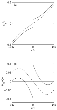
Figure 4: a), Plots of $x_{g}$ versus $\varepsilon$ for a linear combination of two triangles with sizes D=4, D’/D=1/3, $\beta=3$, solid line for a two-sensor COG, dot-dash line for a three-sensor COG, and dotted line for $x_{g}=\varepsilon$. The discontinuities at $\varepsilon=0$ for the two-sensors COG, and at $\varepsilon=\pm 0.5\tau$ for three-sensor COG are clearly visible. In b), the plots of the $(x_{g}-\varepsilon)/\tau$ versus $\varepsilon/\tau$ are shown for both COG, here the discontinuities are more visible.

The three-sensor COG has discontinuities if the range of f$(x)$ (which is $D+\tau_{1}$) is larger than $3\tau$. The discontinuities are located at $\varepsilon=\pm\tau/2$ and often go unnoticed. The points $\varepsilon=\pm\tau/2$ signal the transition from one set of three sensors to another. When $\varepsilon$ approaches $\tau/2$, i.e., the border of the central detector, the signal distribution tends to be symmetric with respect to this point, but the setup of the detectors is asymmetric, and the signal of the leftmost sensor tends to reduce the value of $x_{g}$. When $\varepsilon$ exceeds $\tau/2$, the leftmost sensor is suppressed and sensor is added on the right whose signal tends to increase the value of $x_{g}$ thereby generating a discontinuity. The presence of the discontinuity is signaled in the probability distribution of $x_{g}$ by a reduction in the range of allowed values ($|x_{g}|<\tau/2$). With proper selection of the two sampling functions H$(\omega)$, Eq. (20) produces the discontinuity. Figure 4) plots $x_{g}$ for two and three sensors of relative dimensions sufficient to generate the discontinuities. Discontinuities are present even in the $x_{g}$ calculated with the four, or more, sensors if the size of f$(x)$ is larger than the range covered by the set of detectors. Reference [10] reports discontinuities for various sets of sensors used by the authors. In all these cases, no polynomial approximation of $x_{g}(\varepsilon)$ can cure the systematic error. These singularities, which for even detector numbers are at $\varepsilon=0$ and for odd detector numbers are at $\varepsilon=\tau/2$, render very dangerous the reduction of the noise fluctuation with the subtraction of a "bias". This operation creates an admixture of different algorithms, (e.g., two and three sensors) for $x_{g}$ with very different systematic errors that are almost impossible to correct.

6.5 Probability distribution of $x_{g}$

The above analysis and the explicit calculation of $x_{g}(\varepsilon)$, enables calculating the probability of having a value of $x_{g}(\varepsilon)$. We can compare this probability with experimental histograms obviously keeping in mind the differences discussed in Section 4. For a generic probability distribution P$(\varepsilon)$ of $\varepsilon$ the probability of $x_{g}(\varepsilon)$ is:

$$\Gamma(x_{g})=\mathrm{P}(\varepsilon)\Big{|}\frac{d\varepsilon}{dx_{g}}\Big{|}.$$ (22)

For uniform distribution P$(\varepsilon)$, the probability $\Gamma(x_{g})$ is proportional to the absolute value of the derivative of $\varepsilon$ with respect to $x_{g}$. If the sign of the derivative is the same (nonnegative) in the range of $x_{g}$ values, the absolute value is useless. Now, $x_{g}(\varepsilon)$ can be extracted from $\Gamma(x_{g})$, as done in [16] for the $\eta$-function with a sample of equivalent detectors. We will prove that the sign of $d\varepsilon/dx_{g}$ is non-negative.

With our definitions of $\varphi(x)$, positive, symmetric, and with a single maximum and the property of f$(x)$ to be positive and maintaining a single maximum, $d\varepsilon/dx_{g}$ is always non-negative. Here, we limit ourselves to f$(x)$ and $\varphi(x)$ functions that are continuous, derivable, and have a single maximum and $D>\tau$. More general functions (e.g. rectangular or Dirac $\delta$-functions) will be late explored with the $D<\tau$.

The sign of $d\varepsilon/dx_{g}$ can be determined from the sign of $dx_{g}/d\varepsilon$ which is more accessible. Equations (10) and (13) are not suited to this task, because, being prepared for simulations, their derivative can entail some complication. A functional dependence of $x_{g}$ from $\varepsilon$, better suited to derivatives, can be extracted from Eq. (3) applied to S${}_{\varepsilon}(\omega)$. Here, for uniform crosstalk and without the application of the Poisson identity, S${}_{\varepsilon}(\omega)$ is:

$$\mathrm{S}_{\varepsilon}(\omega)=\sum_{n=-\infty}^{+\infty}\mathrm{f}(n\tau-\varepsilon)\mathrm{e}^{-in\tau\omega}$$

and $x_{g}$ has its standard form:

$$x_{g}(\varepsilon)=\sum_{n=-\infty}^{+\infty}n\tau\mathrm{f}(n\tau-\varepsilon).$$

The derivative respect to $\varepsilon$ is:

$$\frac{dx_{g}(\varepsilon)}{d\varepsilon}=\sum_{n=-\infty}^{+\infty}(-n\tau)\frac{d\mathrm{f}(y)}{dy}\Big{|}_{y=n\tau-\varepsilon}$$

and, for our assumptions regarding the properties of f$(x)$, $dx_{g}/d\varepsilon$ is positive $(D>\tau)$. For $n<0$ $d\mathrm{f}(y)/dy$ is calculated at $y=n\tau-\varepsilon$, i.e., before the maximum, it is positive, giving a positive contribution to the sum. For $n>0$, $d\mathrm{f}(y)/dy$ is calculated at $y=n\tau-\varepsilon$, i.e., after the maximum, it is negative giving a positive contribution to the sum. For $D\leq\tau$, we have $dx_{g}/d\varepsilon=0$ for $\varepsilon=0$.

In the case of the two sensors’ COG and for the range $D$ of $\varphi(x)$ greater than $\tau$, the derivative of $x_{g}$ with respect to $\varepsilon$ must be calculated for $\varepsilon>0$ and $\varepsilon<0$ separately. The derivative for $\varepsilon>0$ is given by:

$$\frac{dx_{g}}{d\varepsilon}=\frac{-\tau(1-x_{g}(\varepsilon)/\tau)}{\mathrm{f}(-\varepsilon)+\mathrm{f}(\tau-\varepsilon)}\frac{d\mathrm{f}(y)}{dy}\Big{|}_{y=\tau-\varepsilon}+\frac{\tau\mathrm{f}(\tau-\varepsilon)}{[\mathrm{f}(-\varepsilon)+\mathrm{f}(\tau-\varepsilon)]^{2}}\frac{d\mathrm{f}(y)}{dy}\Big{|}_{y=-\varepsilon}\quad\varepsilon>0$$

It is positive because $d\mathrm{f}(y)/dy$ at $y=\tau-\varepsilon$ is negative having been calculated after the maximum, $x_{g}/\tau$ is less or equal to 1/2, and $d\mathrm{f}(y)/dy$ at $y=-\varepsilon$ is positive having been calculated before the maximum. For $\varepsilon<0$ we get:

$$\frac{dx_{g}}{d\varepsilon}=\frac{\tau(1+x_{g}(\varepsilon)/\tau)}{\mathrm{f}(-\varepsilon)+\mathrm{f}(-\tau-\varepsilon)}\frac{d\mathrm{f}(y)}{dy}\Big{|}_{y=-\tau-\varepsilon}+\frac{-\tau\mathrm{f}(-\tau-\varepsilon)}{[\mathrm{f}(-\varepsilon)+\mathrm{f}(-\tau-\varepsilon)]^{2}}\frac{d\mathrm{f}(y)}{dy}\Big{|}_{y=-\varepsilon}\quad\varepsilon<0$$

It is positive because $d\mathrm{f}(y)/dy$ at $y=-\tau-\varepsilon$ is positive having been calculated before the maximum, $x_{g}/\tau$ is greater or equal to -1/2, and $d\mathrm{f}(y)/dy$ at $y=-\varepsilon$ is negative having been calculated after the maximum. So, excluding point $\varepsilon=0$ where $x_{g}(\varepsilon)$ has a discontinuity, its derivative is positive and even the derivative of $\varepsilon$ with respect to $x_{g}$ is positive. Likewise, the derivative of $x_{g}(\varepsilon)$ with respect to $\varepsilon$, for the three sensors’ COG is positive, here the discontinuities, if any, are at the edge of the $\varepsilon$-distribution, and do not create complications.

The distribution of probabilities, for two and three sensors is illustrated in Figure 5. The signal distribution used is the same used in Figure 4.

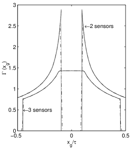
Figure 5: Probability distributions of $x_{g}$ for the two- and three-sensors COG. Solid lines are the analytical calculations. Dot-dash lines join the midsection of a scaled histogram bins generated on a sample of $x_{g}$-data (bin size $x_{g}$/100). The differences are concentrated in the curves’ fast variation regions. The discontinuities of Figure 3 are forbidden $x_{g}$-values.

The dot-dashed lines indicate the histograms normalized to the number of points and bin size. These plots reveal the smearing effect in the regions of fast variation $\Gamma(x_{g})$. This effect must be kept in mind when curves extracted from the above equations are compared with experimental distributions. A dramatic difference could be obtained when $D=\tau$ and $\varphi(\pm\tau/2)=0$, here $\Gamma(0)=+\infty$, no histogram can climb so high.

With our proof of non-negativity of the derivative, Eq. (24) can be used as a differential equation for function $\varepsilon(x_{g})$. The discontinuities of $x_{g}(\varepsilon)$ are no problem for the probability distribution $\Gamma(x_{g})$ because they imply forbidden values for $x_{g}$ with zero probabilities, and, given the probability distribution of $x_{g}$ for a uniform $\varepsilon$ distribution, $\varepsilon(x_{g})$ is given by:

$$\varepsilon(x_{g})=\tau\int_{-\tau/2}^{x_{g}}\Gamma(y)dy-\frac{\tau}{2}.$$ (23)

This generalizes the method introduced in  [16] for the $\eta$-function. The extraction of $\varepsilon(x_{g})$ from the experimental data looks very easy. All we have to do is integrate a histogram of the frequencies of $x_{g}$ for a sample of the equivalent signal distributions and detectors. In using Eq. (25), we must keep in mind two warnings: 1) the fact that the histogram is related to its generating function in a complex way and 2) the fact that noise drastically modifies Eq. (25):

$$\Gamma(x_{g})=\int d\xi_{1},\dots d\xi_{n}\mathrm{P}(\varepsilon(x_{g},\xi_{1},\dots,\xi_{n}))\mathrm{P}(\xi_{1})\dots\mathrm{P}(\xi_{n})\Big{|}\frac{\partial\varepsilon(x,\xi_{1},\dots,\xi_{n})}{\partial x}\Big{|}_{x=x_{g}}.$$ (24)

Now, the extraction of function $\varepsilon(x_{g})$ from this relation is rather complicated, and we have to solve an integral equation. The set of variables $\{\xi_{n}\}$ are the independent sources of noise in the system. For example, in a two-strip COG, three variables are easily encountered. Two variables define the electronic noises of the two strips with a presumably Gaussian distribution. The third variable is the total charge collected by the strips, which has a Landau distribution. For a small amount of noise, Eq. (26) can be solved as Eq. (25) yielding an acceptable approximation of $\varepsilon(x_{g})$. The extraction of $\varepsilon(x_{g})$ from the probability distribution of $x_{g}$ can be fruitfully used to correct the COG sampling error. The presence of noise generally suggests the use of more than a method. The two-sensor COG tends to be less sensitive around $\varepsilon=0$, while conversely, the three-sensor COG is exact for $\varepsilon=0$. Careful simulations should determine the optimal assembly of the two approaches.

Other information can be extracted from $dx_{g}/d\varepsilon$ in the case of infinite sampling, and the absence of crosstalk. Here Eq. (6) can be used, and the functions $x_{g}(\varepsilon)$ and $\varepsilon(x_{g})$ are continuous and derivable ($dx_{g}/d\varepsilon$ is ($\Gamma(x_{g})^{-1}$). Deriving Eq. (6) with respect to $\varepsilon$ gives:

$$\frac{dx_{g}}{d\varepsilon}=1+2\sum_{k=1}^{+\infty}(-1)^{k}\cos\big{(}\frac{2k\pi\varepsilon}{\tau}\big{)}\Phi(\frac{2k\pi}{\tau})$$

which can be reassembled into:

$$\frac{dx_{g}}{d\varepsilon}=\sum_{k=-\infty}^{+\infty}\exp\big{[}i\frac{2k\pi}{\tau}(\epsilon-\frac{\tau}{2})\big{]}\ \Phi(\frac{2k\pi}{\tau})=\tau\sum_{L=-\infty}^{+\infty}\varphi(\varepsilon-\frac{\tau}{2}-L\tau).$$ (25)

The last expression, the Poisson identity, gives the periodic extension of $\varphi(x-\tau/2)$, i.e., sum copies of $\varphi(x-\tau/2)$ shifted by $L\tau$. These equations generalize the results of [16] for any $D$. Now, if the support $D$ of $\varphi(x)$ is less than or equal to $\tau$, the function $\varphi(x)$ is reproduced in the interval $0<x<\tau$. Condition $D\leq\tau$ is signaled by the absence of gaps in $\Gamma(x_{g})$, and an infinite peak at $x_{g}=0$. The peak is given by the zeros of $\varphi(x)$ at $|x|\leq\tau/2$. This pathology cannot be reproduced by any histogram, and the reconstruction of $\varphi(x)$ from experimental distributions unfortunately differ from zero everywhere.

If $D$ is greater than $\tau$, tails of different periods add up and other methods must be used to extract the form of $\varphi(x)$: 1) a couple of sensors are considered together to have an effective $D$ greater than $\tau$ [16], but if crosstalk is present, it can survive the coupling. 2) $x_{g}(\varepsilon)$ is fit with Eq. (13) to get the form factors $\Phi(\gamma_{n})$ and reconstruct $\varphi(x)$ as given in Eq. (9), but no unique results can be expected. 3) $\varepsilon(x_{g})$ is used to reconstruct f$(x)$, and, going backward, to $\varphi(x)$ from Eq. (10) in the absence of crosstalk. Any crosstalk present must be known and Eq. (21) allows the extraction of $\varphi(x)$.

6.6 Other properties of uniform crosstalk: the ideal detector

Equation (27) can be used to fix another property of functions $\varphi(x)$ which are free of the COG discretization error. If $x_{g}=\varepsilon$, than $dx_{g}/d\varepsilon=1$ and we have $\tau\Sigma_{n}(x-n\tau)=1$. Here $D$ is always greater than $\tau$. Functions of this type are introduced in [9] to give consistent meaning to periodic functionals such as that used in Eq. (3). These functions are called unitary functions of range $\tau$. With the unitary functions, it is easy to verify the absence of discretization error for a candidate function. The sum of $\varphi(x)$ with a set of shifted copy must give a unitary function of range $\tau$. This can be verified by a graphic method.

As we mentioned in Section 5.2, the uniform crosstalk functions p$(x,\tau_{1})$ have an identical property (aside from a normalization factor). The conditions for uniform crosstalk are identical to the absence of discretization error which, for uniform crosstalk, must be $\Sigma_{n}$p$(x-n\tau,\tau_{1})=1$. The use of this relation is easier than the FT, and a great number of uniform crosstalk functions can be generated and verified with a simple graphic test.

Let us return to the set of uniform crosstalk functions which are free of discretization error for any signal distribution. The condition for the absence of discretization error can be formulated as a condition on the extended periodic function. Now, p$(x,\tau_{1})$ is uniform crosstalk and $\Sigma_{n}$p$(x-n\tau,\tau_{1})=1$. The derivative $d$P$(\omega,\tau_{1})/d\omega$ must be zero for $\omega=2k\pi/\tau$ $(k=\pm 1,\pm 2,\pm 3,\dots)$ and for $\omega=0$ due to the symmetry of P$(\omega,\tau_{1})$ and p$(x,\tau_{1})$. A series similar to Eq. (27) constructed with this $d$P$(\omega,\tau_{1})/d\omega$ has all the terms equal to zero, and the extended periodic function $\Sigma_{n}(x-n\tau)p(x-n\tau,\tau_{1})$ is also zero.

We can explicitly verify the absence of discretization error using a procedure like that used for uniform crosstalk, but now the sum of the shifted values of $x$p$(x,\tau_{1})$ must give a null function. Starting from Eq. (24) and Eq. (14) for f$(x)$, we can write $x_{g}(\varepsilon)$ as:

$$x_{g}(\varepsilon)=\sum_{n=-\infty}^{+\infty}n\tau\int_{-\infty}^{+\infty}\mathrm{p}(n\tau-\varepsilon-x^{\prime},\tau_{1})\ \varphi(x^{\prime})dx^{\prime}.$$

Interchanging the sum and the integral, adding and subtracting $(\varepsilon+x^{\prime})$ to $n\tau$, and using the uniformity of p$(x,\tau_{1})$, the normalization and symmetry of $\varphi(x)$, we get:

$$x_{g}(\varepsilon)=\varepsilon+\int_{-\infty}^{+\infty}\sum_{n=-\infty}^{+\infty}(n\tau-\varepsilon-x^{\prime})\mathrm{p}(n\tau-\varepsilon-x^{\prime},\tau_{1})\ \varphi(x^{\prime})dx^{\prime}$$

It is now evident that for uniform crosstalk functions with $\Sigma_{n}(x-n\tau)$p$(x-n\tau,\tau_{1})=0$, the discretization error disappears for any signal distribution or can be drastically reduced as p$(x,\tau_{1})$ approximates this condition. It is easy to verify that a triangular function of range $2\tau$ satisfies the condition $\Sigma_{n}(x-n\tau)$p$(x-n\tau,\tau_{1})=0$.

A detector with $\Sigma_{n}(x-n\tau)$p$(x-n\tau,\tau_{1})=0$ will be defined ideal detector; it has $x_{g}(\varepsilon)=\varepsilon$ for any signal distribution.

7 Noise, fluctuations, and border effects

7.1 Noise, cracks, and border effects

The various forms used above for the sampling function allow exploring the efficiency modification and position reconstruction in the presence of several different combinations of experimental setups. Defining h$(x)$ by:

$$\mathrm{h}(x)=a_{-1}\delta(x+\tau+\Delta_{-1})+a_{0}\delta(x-\Delta_{0})+a_{1}\delta(x-\tau-\Delta_{1}),$$

we can simulate the effects of the interstrip calibration errors and the effects of cracks or incorrect detector positions. Properly selecting $\Delta_{-1}$, $\Delta_{0}$, and $\Delta_{1}$, we get H$(\omega)$:

$$\mathrm{H}(\omega)=a_{-1}e^{i\omega(\tau+\Delta_{-1})}+a_{0}e^{-i\omega\Delta_{0}}+a_{1}e^{-i\omega(\tau+\Delta_{1})},$$

H$(\omega)=$H${}^{*}(-\omega)$ and H$(\omega)$ is no longer symmetric in $\omega=0$. Equations (23) and (23’) for S_ε and $x_{g}$ must be modified according to requirements. In this case, the absence of symmetry in the detector array gives a COG systematic error for $\varepsilon=0$ for three detectors and for $\varepsilon=\pm\tau/2$ for two detectors.

Equation (21) enables modifying the response of even a single detector given by the function p$(x,\tau_{1})$, for instance, to evaluate the effects of different quality and size in a row of crystals. In such case, different p$(x,\tau_{1})$ must be considered, and different functions f$(x)$ must be sampled in the proper positions. S${}_{\varepsilon}(\omega)$ becomes:

$$\mathrm{S}_{\varepsilon}(\omega)=\sum_{k=-M_{1}}^{M_{2}}\sum_{n=-\infty}^{+\infty}\Phi_{n}^{p}\ \exp(\frac{-i2n\pi\varepsilon}{T})\ \mathrm{P}_{k}(\frac{2n\pi}{T},\tau_{1})\mathrm{H}_{k}(\omega-\frac{2n\pi}{T})$$

where H${}_{k}(\omega)=a_{k}\exp[-i\omega(\tau_{k}+k)]$; $x_{g}$ is given by:

$$x_{g}=\frac{1}{\mathrm{S}_{\varepsilon}(0)}\sum_{n=-\infty}^{+\infty}\Phi_{n}^{p}\ \exp(\frac{-i2n\pi\varepsilon}{T})\sum_{k=-\infty}^{+\infty}\mathrm{P}_{k}(\frac{2n\pi}{T})a_{k}(\tau_{k}+\Delta_{k})\exp(\frac{i2n\pi(\tau_{k}+\Delta_{k})}{T}).$$

Another fundamental effect to account for in the calculation of the COG is noise. There are essentially two main sources of noise: additive noise due to the readout electronics which modifies the signal collected by each detector, and the fluctuation of $\varphi(x)$ around its average. Let us first consider the readout electronic noise represented as an additive noise. Now, the signals collected by the set of detectors are:

$$\mathrm{sn}_{\varepsilon}(x)=\mathrm{f}^{p}(x-\varepsilon)\big{[}\sum_{m=-M_{1}}^{M_{2}}\delta(x-m\tau)\big{]}+\sum_{m=-M_{1}}^{M_{2}}n_{m}\delta(x-m\tau),$$

where $n_{m}$ are samples taken from the noise distribution scaled by the noise-to-signal ratio, or better by samples of its distribution. This ratio is often far from being a constant. Now, our equations represent a set of isolated points, each defined by its corresponding noise samples. The expressions of the noisy COG $nx_{g}(\varepsilon)$ and the total collected signal NS${}_{\varepsilon}(0)$ are:

$$\mathrm{NS}_{\varepsilon}(0)=\mathrm{S}_{\varepsilon}(0)+\sum_{m=-M_{1}}^{M_{2}}n_{m},$$

$$nx_{g}(\varepsilon)=[x_{g}(\varepsilon)\mathrm{S}_{\varepsilon}(0)+\sum_{m=-M_{1}}^{M_{2}}n_{m}m\tau]/\mathrm{NS}_{\varepsilon}(0),$$

where $x_{g}(\varepsilon)$ and S${}_{\varepsilon}(0)$ are functions considered above in absence of noise.

7.2 Fluctuations

Fluctuation of the signal distribution entails some complications. Generally speaking, we can assume that $D$ is kept fixed, e.g., a little larger than required, and the signal distribution fluctuates as a random function of support $D$. In the case, $\varphi_{r}(x)$ samples of $\varphi(x)$ can be generated with a realistic distribution of the parameters defining $\varphi(x)$. As in Eq. (9), we can put:

$$\varphi_{r}(x)=\frac{1}{D}\Pi(\frac{x}{D})\big{[}\sum_{l=-\infty}^{+\infty}\Gamma_{l}\ \exp(i\frac{2l\pi}{D}x)\big{]},$$

and, for the WKS theorem, the FT becomes:

$$\Phi_{r}(\omega)=\sum_{l=-\infty}^{+\infty}\Gamma_{l}\ \frac{\sin(\omega D/2-l\pi)}{(\omega D/2-l\pi)}$$

with $\Gamma_{l}^{*}=\Gamma_{-l}$ due to the reality of $\varphi_{r}(x)$. The values of $\Phi_{r}(2n\pi/T)$ are the terms to be inserted in Eq.(21) to calculate $x_{g}$ and S${}_{\varepsilon}(0)$. The generation of $\Gamma_{l}$ samples could be a complex operation. Theoretically, the procedure could be to generate $\varphi_{r}(x)$, and than extract the parameters $\Gamma_{l}$ with a FT. By our definitions, the average of all samples $\varphi_{r}(x)$ is $\varphi(x)$.

A possible generation of samples $\varphi_{r}(x)$ for electromagnetic showers can be extraction from the Monte Carlo simulation. We consider an electromagnetic shower developing in a homogeneous medium. The energy released is proportional to the length of the paths of the conversion electrons and positrons. The paths will be approximated to segments of a straight line in the absence of a magnetic bending. The energy released by each segment between two near parallel planes is proportional to the length of the segment trapped between the two planes, and is zero if no segment part is contained. A detailed demonstration is reported in the next section. Observing that the total energy contribution given by a segment is proportional to its length, we find the form of $\varphi_{r}(x)$ given by a set of segments of length $L_{j}$ along $x$, starting from $x_{j}$, and with a total energy contribution $s_{j}$:

$$\varphi_{r}(x)=\frac{1}{\sum_{j}s_{j}}\big{[}\sum_{j}\frac{s_{j}}{L_{j}}\ \Pi(\frac{x-x_{j}-L_{j}/2}{L_{j}})\big{]}.$$ (26)

Its FT $\Phi_{r}(\omega)$ is:

$$\Phi_{r}(\omega)=\frac{1}{\sum_{j}s_{j}}\Big{\{}\sum_{j}s_{j}\ \exp[-i\omega(x_{j}+L_{j}/2)]\ \frac{\sin(\omega L_{j}/2)}{\omega L_{j}/2}\Big{\}}.$$ (27)

The construction of $\varphi_{r}(x)$ and $\Phi_{r}(\omega)$ is now easer. We need to extract a set of values $\{s_{j},x_{j},L_{j}\}$ for each Monte Carlo event, and, accumulating a sufficient number of events, we can generate the average distribution $\omega(x)$ with a realistic sample of fluctuations. For our needs, not all the details of Equations (28) and (29) are worthy of attention. The convolution of $\varphi_{r}(x)$ with the p$(x,\tau_{1})$ is a low-pass filter which considerably smears $\varphi_{r}(x)$. In our approach based on the FT and FS, this means that the sum over a discrete index can be safely cut off at some reasonable value without negatively effecting the results. For this reason, even a statistical generation of the parameters $\{s_{j},x_{j},L_{j}\}$ rougher than a detailed Monte Carlo calculation should suffice for fine-tuning a position reconstruction algorithm.

Lastly, let us examine the asymmetry introduced by the slight ($3^{0}$) off-axis distortion of the crystals of the CMS em-calorimeter. In this case, the average shower is not symmetric: $x_{g}$ and $\varepsilon$ now refer to the shower’s COG, which, when projected on the $x$-axis, does not coincide with the impact point of the photon (or electron/positron) on the calorimeter face. To extract the impact point, we must first correct the discretization on $\varepsilon$. With $\varepsilon$ and the average depth of the shower’s COG, we can calculate the shower’s impact point.

7.3 Signal density for a set of tracks

Let us consider the energy released along the path of a charged particle, assuming that the signal collected is proportional to the length of the path. Neglecting its width, we can represent a charged track as a set of segments of a straight line whose length is $s_{j}$, whose starting point is $\mathbf{r}_{j}\equiv\{x_{j},y_{j},z_{j}\}$ and whose projections on the axis are $\mathbf{L}_{j}\equiv\{X_{j},Y_{j},Z_{j}\}$. The three-dimensional energy distribution of each segment can be written as:

$$\mathrm{e}_{j}(x,y,z)=s_{j}\int_{0}^{1}d\lambda\delta(x-x_{j}-\lambda X_{j})\delta(y-y_{j}-\lambda Y_{j})\delta(z-z_{j}-\lambda Z_{j}).$$ (28)

The energy density collected at point $x$ is given by:

$$\mathrm{e}_{j}(x)=\int_{R^{2}}dydz\mathrm{e}_{j}(x,y,z).$$

Since the function e${}_{j}(x,y,z)$ is too singular to be handled, it is better to use its FT, (E${}_{j}(\mathbf{W})$ is a compact notation for E${}_{j}(\omega_{x},\omega_{y},\omega_{z})$).

$$\mathrm{E}_{j}(\mathbf{W})=\int_{R^{3}}d^{3}r\ \mathrm{e}_{j}(\mathbf{r})\ \exp[-i\mathbf{W\cdot r}]$$

which, substituting Eq. (30), becomes:

$$\mathrm{E}_{j}(\mathbf{W})=s_{j}\int_{0}^{1}d\lambda\ \exp[-i\mathbf{W}\cdot(\mathbf{r}_{j}+\lambda\mathbf{L}_{j})]=\exp[-i\mathbf{W}\cdot(\mathbf{r}_{j}+\mathbf{L}_{j}/2)]\ \frac{\sin(\mathbf{W\cdot L}_{j}/2)}{\mathbf{W\cdot L}_{j}/2}s_{j}.$$

The energy distribution e${}_{j}(x)$ is given by the inverse FT of E${}_{j}(\omega_{x},0,0)$:

$$\mathrm{E}_{j}(\omega_{x},0,0)=s_{j}\ \exp[-i\omega_{x}(x_{j}+X_{j}/2)]\frac{\sin(\omega_{x}X_{j}/2)}{(\omega_{x}X_{j}/2)}.$$

It is evident that E${}_{j}(\omega_{x},0,0)$ is the FT of:

$$\varphi_{j}(x)=\frac{s_{j}}{X_{j}}\ \Pi(\frac{x-x_{j}-X_{j}/2}{X_{j}}).$$

Summing over the $j$-index and normalizing, we get Eq. (28). The periodic extension of $\varphi_{j}^{p}(x)$ can be achieved according to the rule:

$$\varphi_{r}^{p}(x)=\frac{1}{\sum_{j}s_{j}}\sum_{j}\varphi_{j}^{p}(x)=\frac{1}{T\sum_{j}s_{j}}\sum_{n=-\infty}^{+\infty}\sum_{j}\mathrm{E}_{j}(\frac{2n\pi}{T},0,0)\mathrm{e}^{-i2n\pi x/T}$$

Bidimensional distributions can be generated in a similar way. At a reasonable cutoff ($n\approx 200-250$), the interferences among the contributions of different segments smear the corners and suppress the Gibbs effects at each rectangle’s borders in $\varphi_{j}^{p}(x)$ giving very realistic energy distributions. This form plots easier than Eq.(26). To see the aspect of $\varphi_{j}^{p}(x)$, we generate a few random distributions of segments whose lengths follow a Rayleigh distribution averaging around one radiation length.

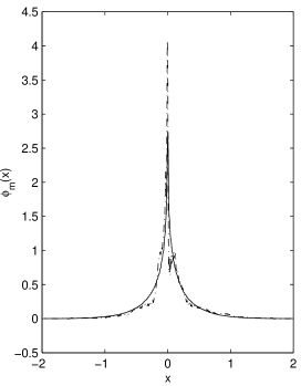
Figure 6: Signal distribution of a set of random segments generated as explained in the text. Dotted line indicates a random sample; solid line is the average of 150 samples. The horizontal scale is in unit of Molier radiuses.

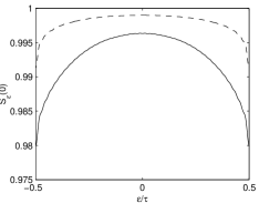
Figure 7: Efficiency plots in function of $\varepsilon/\tau$ for three-sensor (solid line) and five-sensor (dashed line) signal collection, with effective loss of 0.002 at the sensor borders. The sensor size ($\tau$) is 1.1 Molier radius.

Their origins and zenith angles are Gaussian functions with standard deviations respectively ($0.5,\pi/3$). The azimuth angles have uniform distributions. $z$-distributions of the segment origins are irrelevant to this simulation. The average $x$-distribution of the sets of random segments can be made to resemble to the average em shower described in [12]. One of the characteristics they share is the presence of a narrow peak at $x=0$ and a near exponential decrease in the shoulders (Figure 6) . We use this distribution, scaled with the Molier radius, to simulate a more complex signal distribution than that in Eq.(8). Due to some similarity with an em shower, we sampled this signal with sensors of the size (in Molier radiuses) used in the CMS em calorimeter.

Figure 7) shows the efficiencies versus of a set of three and five sensors, with a total loss at the borders of 0.002. Figure 8) shows the systematic error of the two- and three-sensor COG for this signal distribution.  

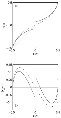
Figure 8: The same plots as Figure 4 for the average signal distribution of Figure 6.

8 Conclusions

We have analytically explored many properties of the center of gravity (COG) algorithm. The effects of the sampling destroy the simple identity of the COG with the symmetry axis of the signal distribution. Few exceptions are worthy of mention. The symmetric functions with band limitation $\Phi(\omega)=0$ for $\omega>2\pi/\tau$ have the sampled COG coincident with the symmetry axis of $\varphi(x)$. This property is shared even by rectangular functions with $D=\tau,2\tau,3\tau,\dots k\tau\dots$ multiples of the sampling interval, the triangular functions with $D=2\tau,4\tau,6\tau\dots$ and all the convolutions of $n$ identical rectangular functions for $D=n\tau,2n\tau,3n\tau\dots$. In all other cases, the COG has a complex nonlinear relation with the symmetry axis of $\varphi(x)$ which can be handled with data involving $\varphi(x)$. An interesting effect is provided by the crosstalk, which is normally considered a sort of undesired distortion introduced in signal collection. It has been proven that the crosstalk can be modulated to have a signal collection whose COG turns out to be free of discretization error for any signal distribution. One of the simplest crosstalk forms with the above property is a triangle with size $2\tau$, but the convolution of any symmetric function with a triangular shape maintains the property. An easy test for the crosstalk function to be of the type described is $\sum_{n}(x-n\tau)$p$(x-n\tau,\tau_{1})=0$. If a large sample of equivalent signal distribution collections is available, it can be used to extract a faithful approximation to $\varepsilon(x_{g})$ from a distribution of $x_{g}$, and, if $D<\tau$, to extract the signal distribution $\varphi(x)$ or the detector response function. If precise position measurements are available, the mismatch of the COG from can be used to access to $\varphi(x)$ or to extract the detector response function. Explicit equations are given for the simulation of the experimental setup, and for the fine-tuning of the algorithm in the presence of discontinuities. The relations of $x_{g}$ with $\varepsilon$ show that the COG, calculated with the suppression of the low-signal detectors, must be carefully handed to avoid the admixtures of different numbers of sensors in the calculation, which, for the different systematic errors, are difficult to correct. Various models of noise and fluctuations are explored with an emphasis on the extraction of signal distributions and averages from a Monte Carlo simulation. Although the equations presented look very complex, they are actually very easy to use. Only a few lines of MATLAB programming language are needed to implement each one and to generate a complete simulation of a measurement setup with noise and fluctuations. All these results remain valid for asymmetric signal distributions, with only negligible modifications to the equations. In this case, $\varepsilon$ indicates the signal distribution’s COG and no longer its impact point which we assumed to coincide with the symmetry axis. The detection of the impact point requires further ad hoc assumptions.

References

- [1] ATLAS Collaboration.CERN-LHCC-94-43.
- [2] CMS Technical Proposal, CMS Collaboration. CERN-LHCC-94-38.
- [3] B. Adeva et al., Nucl. Instrum. and Methods A289 35 (1990).
- [4] CMS Collaboration, The Electromagnetic Calorimeter, CERN/LHCC 1997-33.
- [5] R. Wigmans, Calorimetry (Clarendon Press, Oxford, 2000).
- [6] CMS Collaboration, Tracker Design Report, CERN/LHCC 1998-6.
- [7] O. Adriani et al., Nucl. Instrum. Methods A 409, 447 (1998).
- [8] R.N. Bracewell, The Fourier Transform and Its Application (McGraw-Hill, New York, NY, 1986).
- [9] D.C. Champeney, A Handbook of Fourier Theorems (Cambridge University Press, Cambridge, UK, 1987).
- [10] K. Lau and J. Pyrlik, Nucl. Instrum. Methods A 366, 298 (1995).
- [11] A. J. Jerri Proceedings IEEE 65, 1565 (1977) .
- [12] A.A. Lednev, Nucl. Instrum. Methods A 366, 292 (1995).
- [13] K. Suhling, R. W. Airey, B.L. Morgan, Nucl. Instrum. Methods A 437, 393 (1999).
- [14] P. Henrici, Applied Computational Complex Analysis (John Wiley, New York, NY, 1974).
- [15] B. Alpat et al., Nucl. Instrum. Methods A 439, 53 (2000).
- [16] E. Belau et al., Nucl. Instrum. and Methods 214, 253 (1983).