Positron Annihilation Lifetime Spectroscopy Using Fast Scintillators and Digital Electronics

Abstract

Positron Annihilation Lifetime Spectroscopy (PALS) is a non-destructive radiological technique widely used in material science studies. PALS typically relies on an analog coincidence measurement setup and allows the estimate of the positron lifetime in a material sample under investigation. The positronium trapping at vacancies in the material results in an increased lifetime. In this work, we have developed and optimized a PALS experimental setup using organic scintillators, fast digitizers, and advanced pulse processing algorithms. We tested three pairs of different organic scintillation detectors: EJ-309 liquid, EJ-276 newly developed plastic, and BC-418 plastic, and optimized the data processing parameters for each pair separately. Our high-throughput data analysis method is based on single-pulse interpolation and a constant fraction discrimination (CFD) algorithm. The setup based on the BC-418 detector achieved the best time resolution of $198.3±0.8$ ps. We used such optimized setup to analyze two single-crystal quartz samples and found lifetimes of $156±9$ ps and $366±22$ ps, in good agreement with the characteristic time constants of this material. The proposed experimental set up achieve an excellent time resolution, which makes it possible to accurately characterize material vacancies by discriminating between the lifetimes of either the spin singlet or triplet states of positronium. The optimized data processing algorithms are relevant to all the applications where fast timing is important, such as nuclear medicine and radiation imaging.

1 Introduction

PALS is a well-established non-destructive technique used to study defects and vacancies in a variety of different materials. In a positron annihilation experiment, a positron generating source, such as ²²Na, is typically placed between two identical samples of a material under investigation. ²²Na decays into ²²Ne through ${\beta}^{+}$ decay process, creating a positron and an electron neutrino. ²²Ne then de-excites to its ground state in 3 ps and emits a 1.27 MeV gamma ray. The detection of the 1.27 MeV gamma ray can be used to probe the creation of the positron. The positrons quickly thermalize through scattering and may bind with electrons in the material and form two types of positronium: para-positronium (p-Ps) with spin 0 and ortho-positronium (o-Ps) with spin 1.The p-Ps decays by emitting two 511 keV annihilation photons, while the o-Ps emits three photons in vacuum, as constrained by the conservation of angular momentum. In material lattice, the o-Ps mainly decays via ”pick-off” process where the positron annihilates with a electron with opposed spin in the surrounding material and two 511 keV annihilation photons are created [1]. The elapsed time between the initial production of the positron and the detection of the annihilation photon is therefore a measurement of positronium lifetime in the material under investigation.

The positronium lifetime depends on the material structure. In vacuum, the lifetimes of p-Ps and o-Ps are 125 ps and 142 ns, respectively [2]. The p-Ps lifetime can be affected by the material because the Coulomb interaction between the positronium and material changes the distance between the positron and electron [3]. The o-Ps lifetime in a material is reduced drastically due to the ”pick-off” process. If the material contains voids, vacancies or dislocations, the o-Ps can be trapped and the lifetime will be increased compared to the lifetime in a defect-free material. Thus, the positronium can be used as a probe to investigate the material properties, such as defect density in metals [4] and pore characteristics in porous materials [5]. We may also use the PALS to differentiate between different lattice structures of the same material since the positron lifetime depends on the interaction between the positronium and lattice [6].

Time resolution of the measurement system is crucial to perform an accurate measurement of positronium lifetime. Hodges and colleagues [7] set up a system with 330-ps time resolution but they were unable to resolve the p-Ps component from the spectra. Haruo and Toshio [3] achieved a 160 ps time resolution with four BaF₂ scintillators. However, the slowest component of BaF₂ scintillation light pulse has a decay time of approximately 600 ns, which may cause timing artifacts due to pile-up at high count rates. In this work we compared the timing performance of three different materials and chose the fastest one to perform PALS measurement of single-crystal quartz. In recent years, digital electronics, such as digital oscilloscope [8] and fast digitizer [9], are replacing traditional analog timing modules in PALS experiments. Digital signal processing therefore becomes another important factor affecting the time resolution apart from scintillator properties. We have developed a timing algorithm based on pulse interpolation and optimized the processing parameters for three different organic scintillation detectors.

2 Methods

We measured the time resolution of three different pairs of detectors and selected the pair that exhibited the best time resolution to then perform the PALS experiment. We performed a PALS measurement using a ²²Na source and measured the time distribution of the differences of arrival times between the 1.27 MeV ²²Na decay gamma ray and the 511 keV annihilation gamma ray.

2.1 Time Resolution Measurement

We used the experimental setup shown in Fig. 1 for timing resolution measurement. We performed three measurements with two plastic BC-418, two liquid EJ-309, and two plastic EJ-276 detectors. Table 1 shows the properties of these detectors.

Table 1: Properties of BC-418, EJ-309 and EJ-276 detectors

Detector	Ratio H:C	Base (cm)	Top (cm)	Height (cm)	Density (g/cm3)	Photomultiplier tube	Pulse shape discrimination
BC-418	1.100	3.18	1.27	1.27	1.032	R329-02 by Hamamatsu Photonics	Not capable
EJ-309	1.248	5.08	5.08	5.08	0.959	9214B by Electron Tubes	Capable
EJ-276	0.927	5.08	5.08	5.08	1.096	9214B by Electron Tubes	Capable

The time resolution of each detector pair was estimated as the full-width-at-half-maximum (FWHM) of the distribution of arrival times of two events occurring in coincidence. In this case, the 1.17 MeV and 1.33 MeV gamma rays emitted in cascade by a ⁶⁰Co source are used as reference. A 1µCi ⁶⁰Co disk source was placed between the two detectors under investigation in a sandwich configuration Fig. 1. Approximately 500k counts in coincidence were collected during each measurement. Detected pulses were digitized by the 14-bit 500 MS/s digitizer DT5730 by CAEN Technologies and acquired as full waveforms using the acquisition software CoMPASS [10] with a 200-ns coincidence window. The detectors were powered by the Desktop HV Power Supply Module DT5533EN by CAEN Technologies.

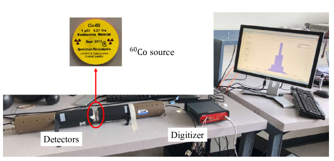
Figure 1: Detector time resolution measurement setup.

We applied the timing algorithm described in Section 2.2 and performed a Gaussian fitting of the time difference distribution to obtain the standard deviation $\sigma$ of the distribution of arrival times and the full width at half maximum (FWHM = 2.355 $\sigma$).

2.2 Timing Algorithm

First, we interpolated the digitized pulses. Digitized pulses were acquired by sampling the analog signal and information about the rising edge and true peak may be partially lost due to insufficient sampling rates. The sampled signal can be reconstructed by convolving the samples with the sinc function if the Nyquist condition is satisfied [11].

$$g(t)=\operatorname{sinc}(t)*g_{s}(t)=\sum_{i=-\infty}^{+\infty}g_{s}(i)\operatorname{sinc}(\frac{t-i\Delta T}{\Delta T})$$ (1)

Here $g_{s}(i)$ is the $i$-th sample, $f=1/\Delta T$ is the sampling rate, and the normalized sinc function is defined as

$$\operatorname{sinc}(x)=\frac{\sin(\pi x)}{\pi x}$$ (2)

If the time interval between sample $j$ and sample $j+1$ is divided into $N$ even parts, then the $k$-th interpolated value between them is given by

$$g(j,k)=\sum_{i=-\infty}^{+\infty}g_{s}(j-i)\operatorname{sinc}(i+k/N)$$ (3)

However, Eq. (3) is not suitable for practical use since the sum extends to infinity and a terminated sinc function is used as the convolution kernel [12], as in Eq. (4)

$$g(j,k)=\sum_{i=-\infty}^{+\infty}g_{s}(j-i)\operatorname{tsinc}(iN+k)$$ (4)

$$\operatorname{tsinc}(i)=\operatorname{sinc}(i/N)\exp(-(i/T)^{2})$$ (5)

Here T is a constant and the Gaussian term quickly drops to 0 as $i$ increases. Thus, the terms in Eq. (4) for sufficiently large values of $i$ can be safely ignored and Eq. (4) reduces to a finite sum [12]

$$g(j,k)=\sum_{i=0}^{L-1}g_{s}(j-i)\operatorname{tsinc}(iN+k)+g_{s}(j+1+i)\operatorname{tsinc}((i+1)N-k)$$ (6)

where $L$ is the width of interpolation window.

Afterwards, we applied a digital version of the constant-fraction discrimination (CFD) algorithm [13] to each interpolated pulse and obtained the zero-crossing bipolar CFD(i) signal.

$$\mathrm{CFD}(i)=F\times S(i)-S(i-\Delta)$$ (7)

In Eq. (7), $S(i)$ is the value of interpolated pulse at index $i$, $F$ and $\mathrm{\Delta}$ are two constants. $F$ is between 0 and 1, and $\mathrm{\Delta}$ is a delay time, which is usually comparable to the pulse rise time. They will be determined later by optimizing the detector time resolution. The zero-crossing point of the bipolar pulse is defined as the time stamp.

We have implemented the above-mentioned algorithms in a ROOT-based pulse-processing program. This software allows us to process 1E6 pulses in approximately 10 seconds using Intel Core i9-7920X @ 2.90GHz.

2.3 PALS Measurement

The PALS experimental setup is shown in Fig. 2. A 10µCi (1-July-2004) ²²Na source was placed in sandwich geometry between two identical single-crystal quartz samples (10mm × 10mm × 1mm each). ²²Na was sealed between two identical Kapton foils. The quartz samples were purchased from MTI Corporation. The two scintillation detectors were placed back to back to achieve the highest detection efficiency. By proper energy gating, detector 0 and detector 1 detected the 1.27 MeV and 511 keV gamma-rays, respectively. We acquired pulses in coincidence, within a 200-ns time window for 12 hours.

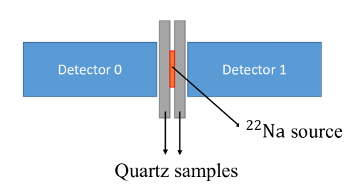
Figure 2: Schematic diagram of the PALS measurement setup using two BC-418 detectors (not to scale).

We applied the timing algorithm to pulses and plotted the positron lifetime spectra. The PALS spectra are usually resolved into three components. The first component results from the decay of p-Ps, the second one from the mixture of decays of o-Ps and free positron, and the third one is due to the delayed decay of o-Ps trapped in defects [6]. The PALS spectrum can therefore be modeled as the convolution of exponential decay function and detector time resolution function, as shown in Eq. (8),

$$f(t)=\sum_{i=1}^{3}\frac{I_{i}}{\tau_{i}}\mathrm{e}^{-\frac{t}{\tau_{i}}}*\frac{\mathrm{e}^{-\frac{t^{2}}{2\sigma^{2}}}}{\sqrt{2\pi\sigma^{2}}}=\sum_{i=1}^{3}\frac{I_{i}}{2\tau_{i}}\mathrm{e}^{\frac{\sigma^{2}-2\tau_{i}t}{2\tau_{i}^{2}}}\mathrm{erfc}(\frac{\sigma^{2}-\tau_{i}t}{\sqrt{2}\sigma\tau_{i}})$$ (8)

where $\tau_{i}$ and $I_{i}$ are the lifetime and intensity of the $i$-th component, $\sigma$ represents the detector time resolution, i.e., FWHM/2.355.

3 Results

3.1 Detector Timing Resolution

Fig. 3 shows the comparison between a interpolated pulse and the original one. The true peak of the original pulse is not captured and only a few sampling points are recorded on the rising edge due to insufficient sampling frequency. Interpolation helps in the characterization of the rising edge by adding more sampling points and gives a more accurate estimate of the true peak. Since CFD relies on the identification of the time corresponding to the maximum value and a fraction of it, the time stamp would be more accurate if we perform CFD after interpolation. As a result, the time resolution would be improved since it is the spread of the arrival times.

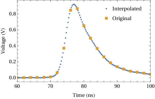
Figure 3: An example pulse before and after interpolation.

Fig. 4 shows the time difference distribution before and after interpolation measured with BC-418 detectors. In Fig. 4(a), we performed Gaussian fitting of the spectra to calculate the FWHM and found that interpolation improved the time resolution by approximately 33 ps. The spectra are not centered at 0 because of the inherent asymmetry of acquisition stages, such as slightly different cable lengths.

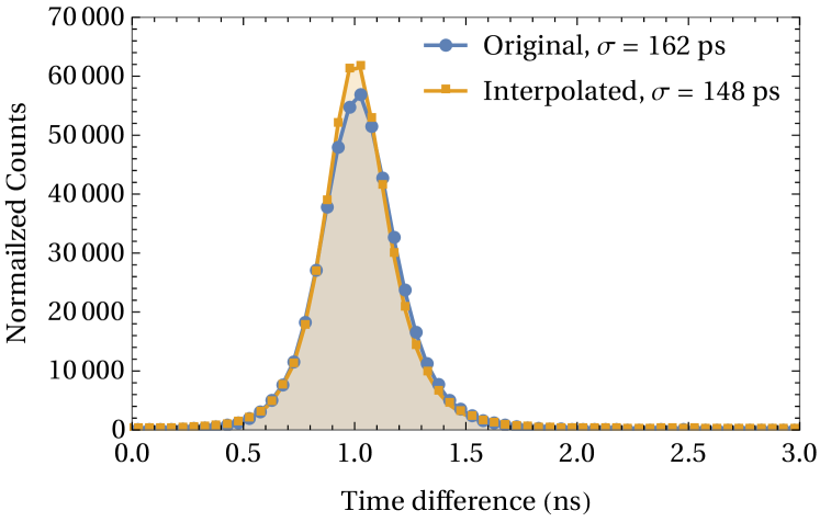
(a) F = 0.75, $\Delta$ = 6 ns

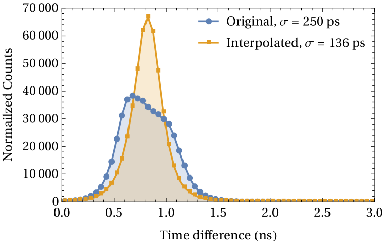
(b) F = 0.4, $\Delta$ = 6 ns

Figure 4: The time difference distribution before interpolation and after interpolation. Measured with BC-418 detectors.

The interpolation algorithm also helps reduce the skewness of the time difference histogram. With $\Delta$ fixed, an over-small F usually leads to a skewed histogram. Fig. 4(b) shows two time difference distributions before and after interpolation, with F = 0.4 and $\Delta$ = 6 ns. After interpolation, the time difference histogram is more symmetrical.

The FWHM of the time difference distribution depends on the DIACFD parameters F and $\Delta$. Fig. 5(a), 5(b), 5(c) illustrate the optimization of F and $\Delta$ for each detector pair. We increased $\Delta$ in steps of 2 ns and for each $\Delta$ we decreased F from 1 until severe artifacts showed up on the spectrum. For each combination of F and $\Delta$ we fitted a Gaussian to the spectrum and calculate the FWHM. Fig. 6 shows the best time resolution of each detector pair. Time resolutions of EJ-276 and EJ-309 are close to each other and BC-418 exhibits the best time resolution. The minimum 195.7 ps $\sigma$ (293.4 ps FWHM) is obtained with BC-418 detectors at F = 0.4 and $\Delta$ = 4 ns.

(a) BC-418

(b) EJ-309

(c) EJ-276

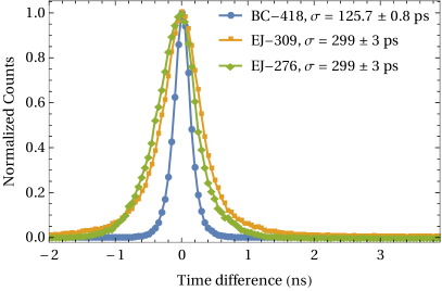
Figure 6: Optimized time resolution

We can further reduce the FWHM by rejecting the low energy pulses. These pulses have small amplitudes and the sampling values could be easily affected by the noise, which leads to large errors of the time stamps and creates a long tail in Fig. 4. After rejecting pulses with deposited energy less than 600 keVee, the minimum FWHM and optimized parameters of each detector pair are summarized in Table 2. The BC-418 detectors yielded the best time resolution and were used in the PALS experiment.

Table 2: Comparison of detector time resolution

Detector	$\Delta$ (ns)	F	$\sigma$ (ps)	FWHM (ps)
BC-418	4	0.4	84.2 ± 0.3	198.3 ± 0.8
EJ-309	10	0.2	172.5 ± 0.3	406.3 ± 0.8
EJ-276	6	0.05	215.1 ± 0.3	507.4 ± 0.7

3.2 Positron Lifetime in Single-Crystal Quartz

Fig. 7 shows the comparison of the positron lifetime spectrum in quartz and the distribution of arrival times obtained using the ⁶⁰Co. The positron lifetime spectrum shows a longer tail due to longer lifetime, as expected.

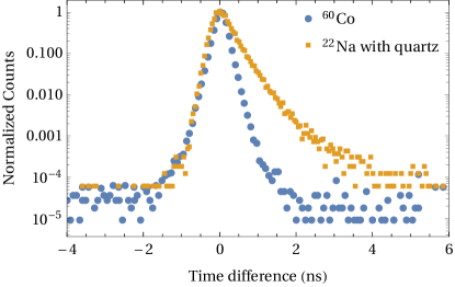
Figure 7: The ⁶⁰Co spectrum and the positron lifetime spectrum in single-crystal quartz, measured with BC-418 detectors.

Our single-crystal quartz samples are of high purity and high internal crystalline perfection. Defects such as micro-bubbles and cracks are not allowed during the manufacturing process. Thus, we believe the third component was actually undetectable and only two components could be identified from the PALS spectrum. We fitted Eq. (6) to the positron lifetime spectrum using the LT10 program [14], which is the one of the most widely used PALS analysis software. The result is shown in Fig. 8. The intensities and lifetimes are shown in Table 3. The lifetimes $\tau_{1}$ and $\tau_{2}$ are 159 ps and 366 ps, respectively, and are in good agreement with the reported values of 156 ps [3] and 358 ps [6]. $\tau_{2}$ shows large standard error due to insufficient amount of counts.

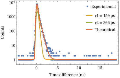
Figure 8: Fit the PAL spectrum of the single-crystal quartz sample.

Table 3: Lifetimes and intensities

Detector	$\tau_{1}$ (ps)	$\tau_{2}$ (ps)	$I_{1}$ (%)	$I_{2}$ (%)
Experiment	159 ± 9	366 ± 22	60 ± 6	40 ± 6
Reference	156 ± 4	357 ± 3	84.2 ± 0.3	15.8 ± 0.3

4 Discussion and Conclusions

We have implemented a digital version of CFD algorithm to accurately determine the onset time of interpolated pulses. We also tested another timing algorithm where we calculated the time when the sampling value exceeds a fixed fraction of pulse height. The reported method showed better timing resolution. Interpolation helps in obtaining a non-skewed time difference distribution and improves the detector timing resolution. There is an optimum value for the F factor, which is between 0.2 and 0.4 for two of the investigated detectors. BC-418 plastic detector exhibited the best time resolution, with a FWHM of 198.3 ± 0.8 ps, because of it’s faster response, its truncated-cone geometry and smaller crystal size. We then used two BC-418 detectors to measure the positron lifetime spectra in single-crystal quartz and we found the positron lifetimes in quartz were 159 ± 9 ps and 366 ± 22 ps. We will use the optimized experimental setup to analyze vacancies and damages created in radiation detectors irradiated at high fluence rates.

References

- [1] W. Brandt, S. Berko, W. W. Walker, Positronium decay in molecular substances, physical review 120 (4) (1960) 1289. doi:10.1103/PhysRev.120.1289.
- [2] D. Gidley, A. Rich, E. Sweetman, D. West, New precision measurements of the decay rates of singlet and triplet positronium, Physical Review Letters 49 (8) (1982) 525. doi:10.1103/PhysRevLett.49.525.
- [3] H. Saito, T. Hyodo, Direct measurement of the parapositronium lifetime in - s i o 2, Physical review letters 90 (19) (2003) 193401. doi:10.1103/PhysRevLett.90.193401.
- [4] J. Kansy, K. Mroczka, J. Dutkiewicz, Pals determination of defect density within friction stir welded joints of aluminium alloys, in: Journal of Physics: Conference Series, Vol. 265, IOP Publishing, 2011, p. 012010. doi:10.1088/1742-6596/265/1/012010.
- [5] D. Gidley, W. Frieze, T. Dull, A. Yee, E. Ryan, H.-M. Ho, Positronium annihilation in mesoporous thin films, Physical Review B 60 (8) (1999) R5157. doi:10.1103/PhysRevB.60.R5157.
- [6] J. D. Van Horn, F. Wu, G. Corsiglia, Y. C. Jean, Asymmetric positron interactions with chiral quartz crystals?, in: Defect and Diffusion Forum, Vol. 373, Trans Tech Publ, 2016, pp. 221–226. doi:10.4028/www.scientific.net/DDF.373.221.
- [7] C. Hodges, B. McKee, W. Triftshäuser, A. Stewart, Umklapp annihilation of positronium in crystals, Canadian Journal of Physics 50 (2) (1972) 103–109. doi:10.1139/p72-019.
- [8] K. Rytsölä, J. Nissilä, J. Kokkonen, A. Laakso, R. Aavikko, K. Saarinen, Digital measurement of positron lifetime, Applied Surface Science 194 (1-4) (2002) 260–263. doi:10.1016/S0169-4332(02)00128-9.
- [9] F. Bečvář, J. Čížek, I. Prochazka, High-resolution positron lifetime measurement using ultra fast digitizers acqiris dc211, Applied Surface Science 255 (1) (2008) 111–114. doi:10.1016/j.apsusc.2008.05.184.
- [10] C. S.pA., CoMPASS Multiparametric DAQ Software for Physics Applications, CAEN S.pA.
- [11] C. E. Shannon, Communication in the presence of noise, Proceedings of the IEEE 86 (2) (1998) 447–457. doi:10.1109/JPROC.1998.659497.
- [12] W. K. Warburton, W. Hennig, New algorithms for improved digital pulse arrival timing with sub-gsps adcs, IEEE Transactions on Nuclear Science 64 (12) (2017) 2938–2950. doi:10.1109/TNS.2017.2766074.
- [13] W. Steinberger, M. Ruch, A. Di-Fulvio, S. Clarke, S. Pozzi, Timing performance of organic scintillators coupled to silicon photomultipliers, Nuclear Instruments and Methods in Physics Research Section A: Accelerators, Spectrometers, Detectors and Associated Equipment 922 (2019) 185–192. doi:10.1016/j.nima.2018.11.099.
- [14] J. Kansy, D. Giebel, Study of defect structure with new software for numerical analysis of pal spectra, in: Journal of Physics: Conference Series, Vol. 265, IOP Publishing, 2011, p. 012030. doi:10.1088/1742-6596/265/1/012030.