An energy consistent discretization of the nonhydrostatic equations in primitive variables
Abstract
We derive a formulation of the nonhydrostatic equations in spherical geometry with a Lorenz staggered vertical discretization. The combination conserves a discrete energy in exact time integration when coupled with a mimetic horizontal discretization. The formulation is a version of \citeADubosTort2014 rewritten in terms of primitive variables. It is valid for terrain following mass or height coordinates and for both Eulerian or vertically Lagrangian discretizations. The discretization relies on an extension to \citeASB81 vertical differencing which we show obeys a discrete derivative product rule. This product rule allows us to simplify the treatment of the vertical transport terms. Energy conservation is obtained via a term-by-term balance in the kinetic, internal and potential energy budgets, ensuring an energy-consistent discretization with no spurious sources of energy. We demonstrate convergence with respect to time truncation error in a spectral element code with a HEVI IMEX timestepping algorithm.
Journal of Advances in Modeling Earth Systems (JAMES)
Computational Science, Sandia National Laboratories, Albuquerque, New Mexico, USA. Department of Land, Air and Water Resources, University of California, Davis, California, USA. NVIDIA, Santa Clara, California, USA Univ. Grenoble Alpes, Inria, CNRS, Grenoble INP, LJK, 38000 Grenoble, France
Mark Taylormataylo@sandia.gov
We give a discrete Hamiltonian formulation of the nonhydrostatic equations in primitive variables.
The formulation supports mass or height terrain following coordinates.
The Lorenz staggered vertical discretization obeys a derivative product rule.
Plain Language Summary
Energy consistent discretizations have proven useful in guiding the development of numerical methods for simulating fluid dynamics. They ensure that the discrete method does not have any spurious sources of energy which can lead to unstable and unrealistic simulations. Here we provide an energy consistent discretization of the equations used by global models of the Earth’s atmosphere. The discretization is written in terms of standard variables in spherical coordinates and supports a wide variety of terrain following vertical coordinates. It can be used with any horizontal discretization that has a discrete version of the integration-by-parts identity.
1 Introduction
We present a discrete formulation of the nonhydrostatic equations designed for use in a global model of the Earth’s atmosphere. It has been implemented in the version of the High Order Method Modeling Environment (HOMME), [Dennis \BOthers. (\APACyear2005), Dennis \BOthers. (\APACyear2012)] used by the Energy Exascale Earth System Model (E3SM), [Golaz \BOthers. (\APACyear2019)]. We follow a Hamiltonian approach so that the formulation will be energetically conservative and consistent in the sense of \citeAGassmannHerzog2008 when coupled with a mimetic horizontal and vertical discretizations. Energy consistency is obtained via a term-by-term balance in the discrete kinetic, internal and potential energy budgets, ensuring an energy conserving discretization with no spurious energy sources or sinks.
Recent examples of energy consistent global atmosphere models running on unstructured grids include [Taylor (\APACyear2011), Gassmann (\APACyear2013), Dubos \BOthers. (\APACyear2015)]. Here we extend the discretization from \citeATaylor11 to the nonhydrostatic equations using a formulation modeled after \citeADubosTort2014. The main difference is that we formulate the Hamiltonian in terms of the commonly used primitive variables in spherical coordinates. This may simplify implementation in existing modeling frameworks. The discretization supports terrain following mass or height coordinates [Kasahara (\APACyear1974)], which differ only in their boundary conditions and one diagnostic equation. It retains a 2D vector invariant form for horizontal transport and advective form for vertical transport, facilitating both Eulerian and vertically Lagrangian [Lin (\APACyear2004)] coordinates in a single code base. In the vertically Lagrangian (mass or height) coordinate, the vertical coordinate surfaces float in such a way as to ensure no mass flux through the surfaces. In the Eulerian (mass or height) coordinate, the transformed equations are solved in an Eulerian reference frame.
For our vertical discretization, we use \citeASB81 vertical differencing with a \citeALorenz1960 staggering. We introduce an extension to SB81 which obeys a discrete derivative product rule in addition to the well known SB81 discrete integral properties. This product rule ensures the discrete vertical transport terms remain energetically neutral despite being in non-Hamiltonian form. The discretization is energetically consistent when used with the shallow atmosphere approximation, total air mass density as a prognostic variable and general moist equations of state, but with a common approximation in the equation for virtual potential temperature.
The formulation is appropriate for any mimetic spatial discretization in spherical geometry such as \citeAthuburn2009numerical,ringler2010unified,TayFour10,cotter2012mixed,thuburn2015primal, Gassmann2018. Mimetic discretizations are those that mimic key integration and annihilator properties of the divergence, gradient and curl operators [Samarskiĭ \BOthers. (\APACyear1981), Nicolaides (\APACyear1992), Shashkov \BBA Steinberg (\APACyear1995), Bochev \BBA Hyman (\APACyear2006)]. They are commonly used in order to preserve the Hamiltonian structure of the continuum equations [Salmon (\APACyear2004), Salmon (\APACyear2007), Gassmann \BBA Herzog (\APACyear2008)]. Here we use a collocated spectral element discretization due to its retention of 4th order accuracy on unstructured spherical grids and its explicit mass matrix which allows for the use of efficient horizontal explicit vertically implicit (HEVI) timestepping. This efficiency comes at the cost of erratic behavior of grid scale waves [Melvin \BOthers. (\APACyear2012), Ainsworth (\APACyear2014)] which are damped as in \citeAullrich2018. We demonstrate convergence with respect to time truncation error with a 5 stage Runge-Kutta IMEX algorithm.
2 Continuum equations in terrain following coordinates
Following \citeAKasahara1974 and \citeALaprise92 we write the equations of motion in a terrain following coordinate and make use of a pseudo-density based on the hydrostatic pressure. Our physical domain will be Earth’s 3D atmosphere in spherical coordinates with latitude , longitude , and radial coordinate . The altitude from an arbitrary reference level is denoted . A terrain following coordinate is defined so that the bottom boundary corresponds to a surface of constant . We denote the velocity with denoting the the horizontal velocity tangent to constant surfaces. For vertical velocity, we use both and , with the standard material derivative. We take as the total air density, the radial unit vector, and as the geopotential with constant gravitational acceleration .
We assume is a monotone function of , so the pseudo-density can be defined in terms of the hydrostatic pressure and density,
with
Vertical integrals of mass and other density weighted quantities are transformed to terrain following coordiantes via
We denote the three-dimensional physical coordinate-independent differential operators in the usual notation, and use
to denote the two-dimensional operators on surfaces [Ullrich \BOthers. (\APACyear2017)].
2.1 Pressure gradient formulation
We can separate the pressure gradient term into vertical and horizontal components, written in terrain following coordinates as
| (1) | ||||
| (2) |
where for compactness we introduce
We use the usual definition of virtual Exner pressure and virtual potential temperature . These are defined in terms of and from the moist atmosphere but using the ideal gas constant for dry air, , and the specific heat at constant pressure for dry air, . These definitions do not imply any assumptions regarding the equation of state and are used to write the pressure gradient as
2.2 Shallow atmosphere equations
We start with a standard form of the nonhydrostatic equations with the shallow atmosphere approximation in terrain following coordinates. Our goal is to derive a energetically consistent discretization for the adiabatic terms, so we initially neglect dissipation, sources and sinks of moisture and other forcing terms. In the full model, dissipation will be added through choice of timestepping and vertical remap algorithms and horizontal hyperviscosity. Following \citeALaprise92, we write the equations as
| (3) | ||||
| (4) | ||||
| (5) | ||||
| (6) | ||||
| (7) |
with Coriolis term .
2.3 Equation of state
To close the equations we need an equation of state in order to compute , which is needed to derive and . As written above, we can support a very general equation of state via the Gibbs potential approach recommended in \citeAThuburn2017. Given a Gibbs potential , with temperature and representing various forms of water, the algebraic system
| (8) | ||||
| (9) |
then defines and implicitly as functions of and . This system can be solved efficiently with Newton iteration.
Here we simplify the equations substantially by assuming that
This is a common assumption for moist air. It neglects small terms, the magnitude of which are discussed in \citeAstaniforth2006. Under this approximation, we can prognose instead of and then the relation is sufficient to close the system. The water species then become passive tracers during the adiabatic part of the dynamics represented by (3)-(7). The equation of state is only needed when coupling with other aspects of the model, such as to compute needed by the physical parameterizations. The approximation can be made independently of the equation of state, but it is more consistent to introduce an approximate Gibbs potential for which and use this potential in all equation of state calculations [Thuburn (\APACyear2017)].
For the simulations presented here, we use an equation of state for dry air, , and water vapor represented by specific humidity . We assume is prognosed by the model’s transport scheme. The Gibbs potential for this equation of state, e.g. \citeA[Appendix A]Vallis2017, leads to with , , where and are the dry air constants defined above, is the ideal gas constants for water vapor and is the specific heat at constant pressure for water vapor. For this equation of state, we have
and in the absence of sources or sinks of moisture ().
We can introduce an approximate Gibbs potential that is consistent with by taking . This representing a 14% error in . With this approximation, , so that and then since .
2.4 Quasi-Hamiltonian Form
We now give the final form of the continuum equations that will be discretized in § 4. We write the thermodynamic equation in conservation form instead of advective form. We also change the formulation slightly so that it is in quasi-Hamiltonian form (See A) which requires the gradient of the full kinetic energy in the momentum equation. The result is
| (10) | ||||
| (11) | ||||
| (12) | ||||
| (13) | ||||
| (14) |
with
| (15) |
where in (15) we have rewritten in terms of our prognostic variables.
2.5 Height coordinate
In the height coordinate, our formulation is valid for any general terrain following coordinate as long as is a monotone function of and independent of time, such as \citeAGalChen1975 and generalizations that allow for a quicker transition from terrain following to pure height such as \citeASchar2002, Leuenberger2010, klemp2011.
For boundary conditions at the model top and surface, we use a free slip condition (). Since throughout the domain, (12) remains a valid equation if we take diagnostic equation for as
| (16) |
Evaluating this equation at the model top and surface we derive the boundary condition
which is combined with (11) to derive boundary conditions for as well.
2.6 Mass coordinate
For the mass coordinate we follow \citeAArakawaLamb1977,SB81 and define via
with zero near the surface and zero near the model top. In this coordinate system, the diagnostic equation for is obtained by integrating (14) in the vertical and making use of to obtain
| (17) |
For boundary conditions at the model top and surface, we use a free slip condition (). Since at the model surface, from (12) we have a boundary condition on ,
which is combined with (11) to derive boundary conditions for at the surface. At the top of the model we have a free surface with a constant pressure .
2.7 Vertically Lagrangian coordinate
We also consider the vertically Lagrangian coordinate from \citeAsjlin04. We assume the vertical levels move so that there is no flow through the levels () and the vertical advection terms are dropped from the equations. In both mass and height options, the diagnostic equation for is no longer valid nor is it needed. Instead, (12) must be used as a prognostic equation for the level positions.
In practice, the floating vertical levels will eventually become too unevenly spaced and every few timesteps we must remap the solution onto a set of more uniform levels. Here we consider energy conservation only during the floating Lagrangian phase. To remap, we typically use a conservative monotone algorithm which will introduce vertical dissipation. To retain energy conservation in the vertically Lagrangian case an energy conserving remap algorithm would have to be adopted.
3 Energy conservation
We first show energy conservation and derive the energy budget in the continuum. We look at the budget term by term to check that we have formulated the equations so that most terms cancel via integration by parts, so that they will also cancel when discretized with a numerical method that has a discrete integration by parts property. As such we must be careful to only perform algebraic steps which will also hold in the discrete system. In this derivation we note a few key terms that require additional numerical properties in order to obtain energy conservation. The analysis in the discrete case will be identical but with integrals replaced by sums and additional care must be taken to account for the vertical staggering.
The kinetic, internal and potential energy of our equations in terrain following coordinates with integration with respect to is given by
| (18) |
with in the mass coodrinate and in the height coordinate. In the mass coordiante, appears in the energy due to the free surface constant pressure boundary condition.
3.1 Potential energy
For the evolution of potential energy in the mass coordinate, we multiply the continuity equation by and the equation by and sum,
| (19) |
The first four terms will integrate to zero, requiring only integration by parts, and the remaining term is the transfer of potential energy to kinetic energy. In the Lorenz staggered case, some care will be needed in the averaging to ensure the first four terms cancel. This equation can be simplified in the Eulerian height coordinate since , but since this term is not zero in the mass coordinate or the vertically Lagrangian height coordinate, we retain this general form.
3.2 Internal energy
For internal energy we have
Assuming exact time integration, this can be simplified to
We can eliminate the mass coordinate boundary term if we integrate the second term by parts in the vertical, leading to
We then take times the equation, times the equations to derive
The first, third and fifth terms represent transfer to kinetic energy and will cancel after integration by parts with similar terms in the kinetic energy equation. In order for the terms involving to cancel, we require
| (20) |
this relation is needed for the advection terms to be energetically neutral. It can be achieved if care is taken in how the vertical advection of is defined, or if we are using a vertically Lagrangian coordinate where these terms do not appear.
3.3 Kinetic energy
For kinetic energy, take the sum of dotted with the equation, times the equation and times the continuity equation. First we consider only the terms related to advection, which should be energetically neutral. After removing two terms that cancel pointwise, we are left with
| (21) |
The first, second, fifth and sixth terms in the above will cancel when integrating over the sphere via integration by parts. The third, forth, seventh and eight terms cancel in the continuum but rely on additional properties that are not obeyed by general mimetic discretizations. They are responsible for a small lack of conservation in \citeA[§ 4.4]Dubos2015. These terms will cancel via special integral properties satisfied by the SB81 discretization [Simmons \BBA Burridge (\APACyear1981), Taylor (\APACyear2011)]. In § 4.1 we show that this result can be obtained more directly by noting that SB81 also has a discrete derivative product rule.
Now consider the remaining terms involving the pressure gradient
| (22) |
The first term balances the identical term in the potential energy equation and the remaining terms balance with similar terms in the internal energy equation.
3.4 Energy consistency
For energy consistency, we require that the discrete equations reproduce three key aspects of the continuum equations: (1) the transport terms are energetically neutral, meaning that they vanish to machine precision when integrated over the domain, (2) the diagnostic equations for the change in total potential, internal and kinetic energies hold in exact time integration and (3) the transfer terms in these diagnostic equations cancel to machine precision. These three requirements ensure that the discretization is not introducing any spurious sources of energy and that total energy will be conserved in exact time integration.
We denote integration over the entire domain with a double integral, representing integration in the vertical with respect to and integration in the horizontal with respect to an area metric . The energy transfer terms in the budget equations are denoted
| (23) |
| (24) |
After integrating the energy budgets derived in the previous subsection, we obtain
| (25) | ||||
| (26) | ||||
| (27) |
Energy conservation requires , which holds via integration-by-parts.
4 Vertical discretization
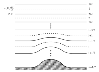
We use a \citeALorenz1960 staggering where the prognostic variables are defined at either level interfaces or midpoints. These levels, their indexing and the staggering of the prognostic variables is shown in Fig. 1. The placement of the prognostic variables then leads to the following natural placement for the remaining variables,
| midpoint quantities: | (28) | |||
| interface quantities: | (29) |
where for convenience we have introduced . The formulas for and mix midpoint and interface quantities, and the averaging necessary for energy consistency will be given in the next section. For the level positions, we require the midpoints to be centered within the interfaces
and denote the level thickness by with
and at the boundaries, and . We note that the coordinate labeling by is arbitrary. The solution will depend on the physical position of each level, but not its assigned -value. For simplicity we could relabel so that for all levels, as is often done in numerical implementations.
Below we will define the averaging and differential operators using a generic variable given at interface points and a generic variable given at midpoints with boundary conditions at the model top and surface . We use standard weighted averaging to map between interface and midpoint quantities. Because of the centered midpoint levels, to average an interface quantities to midpoints we use
| (30) |
and to average (and extrapolate) midpoint quantities to interfaces, we use
| (31) |
This simple extrapolation formula is necessary to ensure a discrete averaging-by-parts identity holds. Vertical derivatives are defined by
| (32) |
with the boundary conditions and one sided differencing used for computing derivatives at the surface and model top
| (33) |
Note that for the operator on midpoint quantities, these boundary conditions must be specified as part of the discretization.
Vertical integrals are approximated via quadrature using a midpoint rule. For midpoint quantities,
| (34) |
and at interfaces
| (35) |
where the prime on the sum is used to denote that we multiply the integrand by at the end points and .
4.1 Discrete operator identities
With these definitions, our discrete operators obey integration and averaging by parts identities as well as a discrete derivative product rule. For interface quantities, averaging commutes with differentiation
| (36) |
with the boundary values of used for the boundary conditions. We have a discrete averaging-by-parts identity
| (37) |
and a discrete integration-by-parts identity
Most importantly for our formulation, and difficult to obtain for general discretizations [Salmon (\APACyear2007)], is the pointwise product rule. For interface quantities and , we have
| (38) |
For midpoint quantities and we have a similar formula, but we have to use unweighted averaging,
| (39) |
where we have extra factors of so that the unweighted average of midpoint quantities is written in terms of the weighted average defined in (31).
4.2 SB81 vertical advection
The SB81 vertical advection for operator is carefully constructed for midpoint quantities in order to conserve energy. We denote this operator with square brackets and write it in terms of interface quantitiy . For midpoint quantities,
| (40) |
For interface quantities, we introduce a generalization of this operator defined by
| (41) |
where we have averaged the midpoint quantity to interfaces. This generalization appears to contain double averaging but it can also be written in an equivalent form without averages of averages.
5 Lorenz staggered formulation
We now write the equations in the vertically staggered discretization using the bar notation for averaging between midpoints and interfaces using (31) or (30), representing (32) and (33) and representing the SB81 transport operator. The discrete equations in their final energy consistent form are
| (42) | ||||
| (43) | ||||
| (44) | ||||
| (45) | ||||
| (46) | ||||
| (47) | ||||
with boundary condition
With this staggering, and at their midpoint locations are determined from (15) without averaging,
and averaging is needed for vertical momentum and ,
In order for the transport terms to be energetically neutral, we need to use special averaging denoted by a tilde for two variables:
| (48) |
For this is the density weighted average. For this represents a version of (15) at interfaces. This term will not be present in the vertically Lagrangian coordinate. In the Eulerian coordinate, (15) at interfaces is thus treated quite differently then (15) at midpoints. As an alternative one can eliminate (15) altogether by introducing an additional prognostic variable for or [Gassmann (\APACyear2013)].
For the mass coordinate, we use a diagnostic integral for ,
and then compute . For the Eulerian height coordinate, we replace the prognostic equation for with the diagnostic equation
and then compute . In the vertically Lagrangian case, and all terms involving these variables are dropped. In the vertically Lagrangian height coordinate, we retain the equation with at the surface and model top held fixed.
We require that the equations for and hold at all interfaces including the model top and surface. This requirement is used to deduce the consistent boundary conditions for and . At the surface, is given for both mass and height coordinates and the equation is satisfied by taking . This allows us to determine at the surface in terms of , which in turn determines the pressure (and equivalently ) at the surface using the prognostic equation for . We omit this algebra here as it depends on details of the spatial discretization. For our purposes, we need only know that and are defined at the surface so that the prognostic equation holds at the surface.
At the model top, for the height coordinate the procedure is identical and and are defined so that the and equations hold at the top most interface. For the mass coordinate, we have a pressure boundary condition and a free surface at the model top. In this case, is well defined and and are evolved at the model top with their prognostic equations.
We note that we used the SB81 operator for vertical advection of and the more traditional discretization for vertical advection of . The SB81 operator is necessary for energy consistency in the momentum equations, but it does not vanish at the surface. The traditional discretization does vanish at the surface since , and its use in the equation results in the more natural boundary condition for .
5.1 Discrete energy conservation
We now repeat the energy budget calculations done for the continuum formulation in § 3. For our horizontal discretization we will be using the mimetic collocated spectral element method from \citeATayFour10. In this case, the horizontal terms which cancel after integration by parts will cancel in the discrete case as well and those calculations are not repeated here. For a horizontally staggered case, such as \citeAthuburn2009numerical, more care must be taken to ensure the horizontal integration by parts properties still hold when mixed with vertical staggering [Gassmann (\APACyear2013)].
5.2 Discrete potential energy
We define discrete potential energy at midpoints
For the budget, we derive the discrete analog of equations (25). We take the continuity equation, average to interfaces and multiply by , and then add in the equation multiplied by . Assuming exact time integration, we have
| (49) |
Similar to the continuum equations, four of these terms will cancel when integrated over the domain after integration by parts and making use of the definition of . The last term, after averaging by parts, becomes,
| (50) |
5.3 Discrete internal energy
We use a discrete internal energy
with in the mass coordinate and in the height coordinate. Differentiating with respect to time, and taking which will hold in exact time integration as well as in the the limit of small , and using that in both coordinate systems,
where we have removed the terms
since our discrete EOS is We then apply integration by parts to obtain
Inserting the discrete prognostic equations,
| (51) |
The first, third and fifth terms make up the transfer terms which will balance similar terms in the kinetic energy equation. For the vertical advection terms, we integrate one term by parts and use the definition of to obtain
Ensuring that these two terms cancel is the reason behind our complex formula for .
5.4 Discrete kinetic energy
Starting with at midpoints,
summing and applying averaging by parts we have
| (52) |
We then derive the discrete budget following § 3.3. We dot the discrete equation for by and sum with times the equation and times the continuity equation. Starting with just the advection terms from (21), we drop four of the terms which cancel after integration by parts in the horizontal and two terms cancel after integration by parts in the vertical, using the SB81 operator for and the product rule identity (39). The remaining advection terms are
| (53) |
Using the definition of from (48) the first two terms cancel. Expanding the SB81 operator and applying integration-by-parts we are left with
To show these two terms cancel, we apply the SB81 product rule, average by parts, apply (36) and then integrate by parts making use of at the boundaries,
| (54) |
Finally, we are left with the discrete version of the transfer terms from (22),
| (55) |
5.5 Discrete energy consistency
We now write the discrete integral energy budgets. Let the sum over represent the vertical integral as above. In the horizontal, we let the sum over represent the discrete quadrature for integration over spherical surfaces associated with the mimetic horizontal discretization.
| (56) |
| (57) |
| (58) |
| (59) |
After integrating the energy budgets derived in the previous subsection, we obtain
| (60) | ||||
| (61) | ||||
| (62) |
To obtain energy conservation, we note that after integration by parts and after averaging-by-parts. To show we average by parts and then expand and . Ensuring is the motivation behind the averaging of in the momentum equation. This is the only term in our formulation that contains double averaging (since contains an average of ). This is unavoidable given our definition of needed to obtain energy neutral transport.
6 Numerical implementation
We have implemented the discretization described here in an open source version of HOMME. HOMME previously contained a shallow water and hydrostatic primitive equation model and we use HOMME-NH to refer to the new nonhydrostatic model. For the horizontal directions, HOMME-NH relies on the existing HOMME infrastructure including the mimetic spectral element discretization, monotone and conservative tracer transport [Guba \BOthers. (\APACyear2014)], and support for fully unstructured arbitrary quadrilateral grids [Guba \BOthers. (\APACyear2014b)]. Here we will be running the model on the quasi-uniform equi-angle cubed sphere grid [Ronchi \BOthers. (\APACyear1996)]. Within each spectral element we use 4th order accurate polynomial basis functions of degree .
HOMME-NH implements (42)–(47) using method of lines. The horizontal divergence, gradient and curl operators on -surfaces are evaluated with existing HOMME subroutines, and the vertical terms are computed as written. All the tendency terms are computed locally within each element and then we apply a standard finite element assembly step. Because of the spectral element method’s diagonal mass matrix, this assembly is explicit and can be computed in each element with only nearest neighbor information. For our initial HOMME-NH implementation we use the mass coordinate for with both Eulerian and vertically Lagrangian options. For the vertically Lagrangian option, we typically remap back to the initial reference levels every three timesteps using parabolic splines [Zerroukat \BOthers. (\APACyear2006)].
For timestepping, we use a HEVI approach [Satoh (\APACyear2002)] discretized with a Runge-Kutta IMEX method. The HEVI/IMEX combination has proven attractive for atmospheric models, e.g. \citeAUllrichJablonowski2012,GKC2013,Weller2013,Lock2014. HOMME-NH supports a variety of IMEX methods from the ARKODE package [Gardner \BOthers. (\APACyear2017), Gardner \BOthers. (\APACyear2018)] of the SUNDIALS library [Hindmarsh \BOthers. (\APACyear2005)]. Here we use a 5 stage 2nd order accurate high-CFL method derived in \citeASteyer2019. In the HEVI approach, the vertically implicit component can be solved independently in each vertical column. We use Newton iterations with the Jacobian computed analytically and inverted by direct LU factorization. We use a time-split approach to couple (42)–(47) with hyperviscosity and physical parameterizations following \citeADennis12.
HOMME-NH is further described in [Ullrich \BOthers. (\APACyear2017)] and results from a splitting supercell thunderstorm test case are given in [Zarzycki \BOthers. (\APACyear2019)].
7 Numerical results
We use HOMME-NH to verify the three energy consistent properties from § 3.4. Properties (1) and (3) depend on the mimetic properties of the discretization. These are verified through unit tests for all the terms in the energy budgets which should cancel when integrated over the domain. These tests are useful for ensuring all differential operators and quadrature rules are properly coded and are not presented here. To establish property (2) we verify that equations (60)-(62) are satisfied to within time truncation error when running HOMME-NH without forcing or explicit dissipation. Since these equations would be exact in exact time integration, their residual is a measure of the dissipation introduced by the time stepping algorithm. In an energy consistent discretization, this dissipation should converge to zero with .
We make use of a moist baroclinic instability test case from the Dynamical Core Model Intercomparison Project (DCMIP) [Ullrich \BOthers. (\APACyear2017), Ullrich \BOthers. (\APACyear2018b)]. This test case is based on \citeAullrich2014 with the addition a prognostic variable for specific humidity and the \citeAReed2012 simple physics package. The physics includes large-scale condensation, surface fluxes and boundary layer turbulence. We use a low resolution grid with average grid spacing at the Equator and 30 vertical levels. This low resolution ensures energy conservation holds even in the presense of large spatial truncation errors.
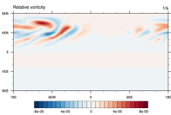
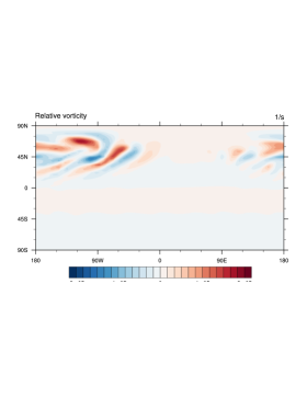
To analyze the HOMME-NH discretization with a realistic flow containing energy in all resolved scales we first run the full model for 15 days. The solution at 15 days is shown in Figures 2 and 3. We then disable the forcing and all explicit model dissipation and run to time 2 hours. We use the two hour period to study the HOMME-NH solution to the adiabatic component of the model, equations (42)–(47).
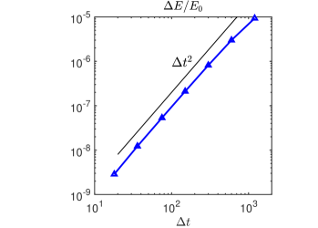
The energy conservation of the discretization as a function of is shown in Fig.4. We plot the relative change in total energy over
for simulations with ranging from close to the CFL stability limit (1200s) down to 18s. With a second order accurate time stepping algorithm we expect second order convergence in the energy, as shown.

Next we examine the residual error for (60)-(62) instantaneously at time given by
| (63) | ||||
| (64) | ||||
| (65) |
The residuals and represent unphysical changes in potential, internal and kinetic energy in HOMME-NH as a function of . For simplicity we estimate with a first order accurate approximation so that and can be computed in the code at each timestep with only data from that timestep. In Fig.5 we plot and , with again ranging from the CFL limit (1200s) to 18s. From the figure we see that and decrease to zero as , as expected due to our first order approximation. The value of is 3 orders of magnitude smaller than and , and decreases to zero at an even faster rate until reaching machine precision. For this problem, and are always negative, is always positive, , and . At , corresponds to change in the 12’th digit of . These results verify the HOMME-NH implementation of (42)–(47), confirming that the spatial discretization does not have any spurious sources of energy and that the only changes in energy are due to the timestepping algorithm.
Most simulations with HOMME-NH are run with timesteps close to the CFL limit. In this regime, we see that the dissipation from time truncation is at day 15. To compare this number with dissipation from the non-adiabatic terms, we note that at day 15 before the explicit dissipation was turned off, the kinetic energy dissipation from hyperviscsoity and the vertical remap is and respectively.
8 Conclusions
We have presented a discretization of the nonhydrostatic equations in terrain following coordinates with a Lorenz staggered vertical discretization. The discretization is energy consistent in exact time integration when coupled with a mimetic horizontal discretization, meaning the discrete diagnostic equations for potential, internal and kinetic energy are consistent and total energy is conserved to time truncation error. It supports both mass and height coordinates, which differ only in the top of model boundary condition and the diagnostic equation for . Vertical transport is kept in advective form, leading to unified support for both Eulerian or vertically Lagrangian coordinates. We use virtual potential temperature and prognose total mass to support general moist equations of state. The mass coordinate formulation has been implemented in HOMME-NH, with energy consistency verified using a moist baroclinic instability test case and a Runge-Kutta IMEX timestepping algorithm. In the design of HOMME-NH, we have found energy consistency to be a useful guiding principal that enhances the stability of the discretization. The ultimate goal is not exact energy conservation, but to preserve the Hamiltonian structure of the equations and ensure all changes in energy are through explicitly added dissipative mechanisms. In HOMME, these mechanisms include hyperviscosity in the horizontal, monotone remap in the vertical and dissipation inherent in the Runge-Kutta method. HOMME-NH is currently being evaluated with a suite of test cases from the DCMIP. Future work will be to add support for the height coordinate and coupling with the Energy Exascale Earth System Model’s suite of atmospheric parameterizations.
Appendix A Quasi-Hamiltonian form
Following \citeADubosTort2014, we show that (10)-(14) is in quasi-Hamiltonian form plus the addition of an energetically neutral vertical transport term . Let
and take
with and defined as in § 3. To find the functional derivatives of we differentiate with respect to time as in § 3 to obtain
| (66) |
and thus
| (67) | ||||
| (68) | ||||
| (69) | ||||
| (70) | ||||
| (71) |
Using these functional derivatives, the equations of motion can be re-written as
This can be seen to fall into the quasi-Hamiltonian form
with a skew symmetric operator defined via
| (72) |
where and
| (73) |
We call this quasi-Hamiltonian form since no attempt has been made to prove the Jacobi identity for . Energy is conserved due the skew-symmetry of and the condition
| (74) |
where
| (75) |
is the adjoint of . The (74) condition is a consequence of the vertical relabeling symmetry of the flow and implies the vertical transport is energetically neutral for any velocity with boundary conditions .
A general mimetic discretization will preserve the skew-symmetry of , but additional properties are needed to obtain a discrete version of (74). To see this, we insert the functional derivatives into
| (76) |
to obtain
| (77) |
The product rule for immediately gives cancellation for the , and terms, leaving only
| (78) |
Now recalling that and
| (79) |
which holds in the continuum due to the definition of and . We can thus obtain a discrete version of (74) with the the SB81 product rule (38) and the special averaging in (48).
Acknowledgements.
HOMME-NH is part of the open source E3SM project with source code publically available from https://github.com/E3SM-Project/E3SM. Instructions for configuring and compiling standalone HOMME-NH are in the README Files in components/homme. Once the model has been configured, the checkE.sh script in dcmip_tests/dcmip2016_test1_baroclinic_wave/theta-l will generate all necessary input data and run the simulations described in this work. This research was supported as part of the Energy Exascale Earth System Model (E3SM) project, funded by the U.S. Department of Energy, Office of Science, Office of Biological and Environmental Research. Sandia National Laboratories is a multimission laboratory managed and operated by National Technology & Engineering Solutions of Sandia, LLC, a wholly owned subsidiary of Honeywell International Inc., for the U.S. Department of Energy’s National Nuclear Security Administration under contract DE-NA0003525. This paper describes objective technical results and analysis. Any subjective views or opinions that might be expressed in the paper do not necessarily represent the views of the U.S. Department of Energy or the United States Government. Christopher Eldred was supported by the French National Research Agency through contract ANR-14-CE23-0010 (HEAT).References
- Ainsworth (\APACyear2014) \APACinsertmetastarainsworth2014{APACrefauthors}Ainsworth, M. \APACrefYearMonthDay2014. \BBOQ\APACrefatitleDispersive behaviour of high order finite element schemes for the one-way wave equation Dispersive behaviour of high order finite element schemes for the one-way wave equation.\BBCQ \APACjournalVolNumPagesJournal of Computational Physics2591–10. \PrintBackRefs\CurrentBib
- Arakawa \BBA Lamb (\APACyear1977) \APACinsertmetastarArakawaLamb1977{APACrefauthors}Arakawa, A.\BCBT \BBA Lamb, V. \APACrefYearMonthDay1977. \BBOQ\APACrefatitleComputational design of the basic dynamical processes in the UCLA general circulation model Computational design of the basic dynamical processes in the UCLA general circulation model.\BBCQ \BIn J. Chang (\BED), \APACrefbtitleMethods in computational physics. Vol. 17: General circulation models of the atmosphere Methods in computational physics. vol. 17: General circulation models of the atmosphere (\BPGS 174–264). \APACaddressPublisherAcademic Press. \PrintBackRefs\CurrentBib
- Bochev \BBA Hyman (\APACyear2006) \APACinsertmetastarbh2006{APACrefauthors}Bochev, P.\BCBT \BBA Hyman, M. \APACrefYearMonthDay2006. \BBOQ\APACrefatitlePrinciples of compatible discretizations Principles of compatible discretizations.\BBCQ \BIn D\BPBIN. Arnold, P. Bochev, R. Lehoucq, R. Nicolaides\BCBL \BBA M. Shashkov (\BEDS), \APACrefbtitleCompatible Discretizations, Proceedings of IMA Hot Topics Workshop on Compatible Discretizations Compatible Discretizations, proceedings of ima hot topics workshop on compatible discretizations (\BVOL IMA 142, \BPGS 89–120). \APACaddressPublisherSpringer Verlag. \PrintBackRefs\CurrentBib
- Cotter \BBA Shipton (\APACyear2012) \APACinsertmetastarcotter2012mixed{APACrefauthors}Cotter, C\BPBIJ.\BCBT \BBA Shipton, J. \APACrefYearMonthDay2012. \BBOQ\APACrefatitleMixed finite elements for numerical weather prediction Mixed finite elements for numerical weather prediction.\BBCQ \APACjournalVolNumPagesJournal of Computational Physics231217076–7091. \PrintBackRefs\CurrentBib
- Dennis \BOthers. (\APACyear2012) \APACinsertmetastarDennis12{APACrefauthors}Dennis, J., Edwards, J., Evans, K., Guba, O., Lauritzen, P., Mirin, A.\BDBLWorley, P\BPBIH. \APACrefYearMonthDay2012. \BBOQ\APACrefatitleCAM-SE: A scalable spectral element dynamical core for the Community Atmosphere Model CAM-SE: A scalable spectral element dynamical core for the community atmosphere model.\BBCQ \APACjournalVolNumPagesInt. J. High Perf. Comput. Appl.2674–89. \PrintBackRefs\CurrentBib
- Dennis \BOthers. (\APACyear2005) \APACinsertmetastarDennis05{APACrefauthors}Dennis, J., Fournier, A., Spotz, W\BPBIF., St.-Cyr, A., Taylor, M\BPBIA., Thomas, S\BPBIJ.\BCBL \BBA Tufo, H. \APACrefYearMonthDay2005. \BBOQ\APACrefatitleHigh Resolution Mesh Convergence Properties and Parallel Efficiency of a Spectral Element Atmospheric Dynamical Core High resolution mesh convergence properties and parallel efficiency of a spectral element atmospheric dynamical core.\BBCQ \APACjournalVolNumPagesInt. J. High Perf. Comput. Appl.19225–235. \PrintBackRefs\CurrentBib
- Dubos \BOthers. (\APACyear2015) \APACinsertmetastarDubos2015{APACrefauthors}Dubos, T., Dubey, S., Tort, M., Mittal, R., Meurdesoif, Y.\BCBL \BBA Hourdin, F. \APACrefYearMonthDay2015. \BBOQ\APACrefatitleDYNAMICO-1.0, an icosahedral hydrostatic dynamical core designed for consistency and versatility Dynamico-1.0, an icosahedral hydrostatic dynamical core designed for consistency and versatility.\BBCQ \APACjournalVolNumPagesGeoscientific Model Development8103131–3150. \PrintBackRefs\CurrentBib
- Dubos \BBA Tort (\APACyear2014) \APACinsertmetastarDubosTort2014{APACrefauthors}Dubos, T.\BCBT \BBA Tort, M. \APACrefYearMonthDay2014. \BBOQ\APACrefatitleEquations of atmospheric motion in non-eulerian vertical coordinates: Vector-invariant form and quasi-hamiltonian formulation Equations of atmospheric motion in non-eulerian vertical coordinates: Vector-invariant form and quasi-hamiltonian formulation.\BBCQ \APACjournalVolNumPagesMonthly Weather Review142103860–3880. \PrintBackRefs\CurrentBib
- Gal-Chen \BBA Somerville (\APACyear1975) \APACinsertmetastarGalChen1975{APACrefauthors}Gal-Chen, T.\BCBT \BBA Somerville, R\BPBIC. \APACrefYearMonthDay1975feb. \BBOQ\APACrefatitleOn the use of a coordinate transformation for the solution of the Navier-Stokes equations On the use of a coordinate transformation for the solution of the navier-stokes equations.\BBCQ \APACjournalVolNumPagesJournal of Computational Physics172209–228. {APACrefDOI} 10.1016/0021-9991(75)90037-6 \PrintBackRefs\CurrentBib
- Gardner \BOthers. (\APACyear2018) \APACinsertmetastarARKODE2018{APACrefauthors}Gardner, D., Guerra, J., Hamon, F., Reynolds, D., Ullrich, P\BPBIA.\BCBL \BBA Woodward, C. \APACrefYearMonthDay2018. \BBOQ\APACrefatitleImplicit-explicit (IMEX) Runge-Kutta methods for non-hydrostatic atmospheric models Implicit-explicit (IMEX) Runge-Kutta methods for non-hydrostatic atmospheric models.\BBCQ \APACjournalVolNumPagesGeosci. Model Dev.111497-1515. {APACrefDOI} 10.5194/gmd-2017-285 \PrintBackRefs\CurrentBib
- Gardner \BOthers. (\APACyear2017) \APACinsertmetastarGardner2017{APACrefauthors}Gardner, D., Reynolds, D., Hamon, F., Woodward, C., Ullrich, P\BPBIA., Guerra, J.\BDBLBanide, A. \APACrefYearMonthDay2017. \BBOQ\APACrefatitleTempest+ARKode IMEX Tests Tempest+ARKode IMEX tests.\BBCQ \APACjournalVolNumPagesGeosci. Model Dev.. {APACrefDOI} 10.5281/zenodo.1162309 \PrintBackRefs\CurrentBib
- Gassmann (\APACyear2013) \APACinsertmetastarGassmann2013{APACrefauthors}Gassmann, A. \APACrefYearMonthDay2013. \BBOQ\APACrefatitleA global hexagonal C-grid non-hydrostatic dynamical core (ICON-IAP) designed for energetic consistency A global hexagonal c-grid non-hydrostatic dynamical core (icon-iap) designed for energetic consistency.\BBCQ \APACjournalVolNumPagesQuarterly Journal of the Royal Meteorological Society139670152–175. \PrintBackRefs\CurrentBib
- Gassmann (\APACyear2018) \APACinsertmetastarGassmann2018{APACrefauthors}Gassmann, A. \APACrefYearMonthDay2018. \BBOQ\APACrefatitleDiscretization of generalized Coriolis and friction terms on the deformed hexagonal C-grid Discretization of generalized coriolis and friction terms on the deformed hexagonal c-grid.\BBCQ \APACjournalVolNumPagesQuarterly Journal of the Royal Meteorological Society1447162038-2053. {APACrefDOI} 10.1002/qj.3294 \PrintBackRefs\CurrentBib
- Gassmann \BBA Herzog (\APACyear2008) \APACinsertmetastarGassmannHerzog2008{APACrefauthors}Gassmann, A.\BCBT \BBA Herzog, H\BHBIJ. \APACrefYearMonthDay2008. \BBOQ\APACrefatitleTowards a consistent numerical compressible non-hydrostatic model using generalized Hamiltonian tools Towards a consistent numerical compressible non-hydrostatic model using generalized Hamiltonian tools.\BBCQ \APACjournalVolNumPagesQuart. J. R. Meteorol. Soc.1346351597–1613. {APACrefDOI} 10.1002/qj.297 \PrintBackRefs\CurrentBib
- Giraldo \BOthers. (\APACyear2013) \APACinsertmetastarGKC2013{APACrefauthors}Giraldo, F., Kelly, J.\BCBL \BBA Constantinescu, E. \APACrefYearMonthDay2013. \BBOQ\APACrefatitleImplicit-Explicit Formulations of a Three-Dimensional Nonhydrostatic Unified Model of the Atmosphere (NUMA) Implicit-explicit formulations of a three-dimensional nonhydrostatic unified model of the atmosphere (NUMA).\BBCQ \APACjournalVolNumPagesSIAM J. Sci. Comput.35B1162-B1194. {APACrefDOI} 10.1137/120876034 \PrintBackRefs\CurrentBib
- Golaz \BOthers. (\APACyear2019) \APACinsertmetastarGolaz2019{APACrefauthors}Golaz, J\BHBIC., Caldwell, P\BPBIM., Roekel, L\BPBIP\BPBIV., Petersen, M\BPBIR., Tang, Q., Wolfe, J\BPBID.\BDBLZhu, Q. \APACrefYearMonthDay2019\APACmonth03. \BBOQ\APACrefatitleThe DOE E3SM coupled model version 1: Overview and evaluation at standard resolution The DOE e3sm coupled model version 1: Overview and evaluation at standard resolution.\BBCQ \APACjournalVolNumPagesJournal of Advances in Modeling Earth Systems. {APACrefDOI} 10.1029/2018ms001603 \PrintBackRefs\CurrentBib
- Guba \BOthers. (\APACyear2014) \APACinsertmetastarGuba2014{APACrefauthors}Guba, O., Taylor, M.\BCBL \BBA St.-Cyr, A. \APACrefYearMonthDay2014. \BBOQ\APACrefatitleOptimization based limiters for the spectral element method Optimization based limiters for the spectral element method.\BBCQ \APACjournalVolNumPagesJ. Comput. Phys.267176–195. {APACrefDOI} 10.1016/j.jcp.2014.02.029 \PrintBackRefs\CurrentBib
- Guba \BOthers. (\APACyear2014b) \APACinsertmetastarGuba2014tensor{APACrefauthors}Guba, O., Taylor, M., Ullrich, P\BPBIA., Overfelt, J.\BCBL \BBA Levy, M. \APACrefYearMonthDay2014b. \BBOQ\APACrefatitleThe spectral element method on variable resolution grids: Evaluating grid sensitivity and resolution-aware numerical viscosity The spectral element method on variable resolution grids: Evaluating grid sensitivity and resolution-aware numerical viscosity.\BBCQ \APACjournalVolNumPagesGeosci. Model Dev.74081-4117. {APACrefDOI} 10.5194/gmdd-7-4081-2014 \PrintBackRefs\CurrentBib
- Hindmarsh \BOthers. (\APACyear2005) \APACinsertmetastarhindmarsh2005sundials{APACrefauthors}Hindmarsh, A., Brown, P., Grant, K., Lee, S., Serban, R., Shumaker, D.\BCBL \BBA Woodward, C. \APACrefYearMonthDay2005. \BBOQ\APACrefatitleSUNDIALS: Suite of nonlinear and differential/algebraic equation solvers SUNDIALS: Suite of nonlinear and differential/algebraic equation solvers.\BBCQ \APACjournalVolNumPagesACM T. Math. Software313363–396. \PrintBackRefs\CurrentBib
- Kasahara (\APACyear1974) \APACinsertmetastarKasahara1974{APACrefauthors}Kasahara, A. \APACrefYearMonthDay1974. \BBOQ\APACrefatitleVarious vertical coordinate systems used for numerical weather prediction Various vertical coordinate systems used for numerical weather prediction.\BBCQ \APACjournalVolNumPagesMon. Wea. Rev.102509–522. \PrintBackRefs\CurrentBib
- Klemp (\APACyear2011) \APACinsertmetastarklemp2011{APACrefauthors}Klemp, J\BPBIB. \APACrefYearMonthDay2011jul. \BBOQ\APACrefatitleA Terrain-Following Coordinate with Smoothed Coordinate Surfaces A terrain-following coordinate with smoothed coordinate surfaces.\BBCQ \APACjournalVolNumPagesMonthly Weather Review13972163–2169. {APACrefDOI} 10.1175/mwr-d-10-05046.1 \PrintBackRefs\CurrentBib
- Laprise (\APACyear1992) \APACinsertmetastarLaprise92{APACrefauthors}Laprise, R. \APACrefYearMonthDay1992. \BBOQ\APACrefatitleThe Euler equations of motion with hydrostatic pressure as an independent variable The euler equations of motion with hydrostatic pressure as an independent variable.\BBCQ \APACjournalVolNumPagesMonthly weather review1201197–207. \PrintBackRefs\CurrentBib
- Leuenberger \BOthers. (\APACyear2010) \APACinsertmetastarLeuenberger2010{APACrefauthors}Leuenberger, D., Koller, M., Fuhrer, O.\BCBL \BBA Schär, C. \APACrefYearMonthDay2010sep. \BBOQ\APACrefatitleA Generalization of the SLEVE Vertical Coordinate A generalization of the SLEVE vertical coordinate.\BBCQ \APACjournalVolNumPagesMonthly Weather Review13893683–3689. {APACrefDOI} 10.1175/2010mwr3307.1 \PrintBackRefs\CurrentBib
- Lin (\APACyear2004) \APACinsertmetastarsjlin04{APACrefauthors}Lin, S\BHBIJ. \APACrefYearMonthDay2004. \BBOQ\APACrefatitleA Vertically Lagrangian Finite-Volume Dynamical Core for Global Models A vertically lagrangian finite-volume dynamical core for global models.\BBCQ \APACjournalVolNumPagesMon. Wea. Rev.1322293–2397. \PrintBackRefs\CurrentBib
- Lock \BOthers. (\APACyear2014) \APACinsertmetastarLock2014{APACrefauthors}Lock, S\BHBIJ., Wood, N.\BCBL \BBA Weller, H. \APACrefYearMonthDay2014. \BBOQ\APACrefatitleNumerical analyses of Runge-Kutta implicit-explicit schemes for horizontally explicit, vertically implicit solutions of atmospheric models Numerical analyses of Runge-Kutta implicit-explicit schemes for horizontally explicit, vertically implicit solutions of atmospheric models.\BBCQ \APACjournalVolNumPagesQ. J. Roy. Meteor. Soc.1401654-1669. {APACrefDOI} 10.1002/qj.2246 \PrintBackRefs\CurrentBib
- Lorenz (\APACyear1960) \APACinsertmetastarLorenz1960{APACrefauthors}Lorenz, E\BPBIN. \APACrefYearMonthDay1960. \BBOQ\APACrefatitleEnergy and numerical weather prediction Energy and numerical weather prediction.\BBCQ \APACjournalVolNumPagesTellus124364–373. \PrintBackRefs\CurrentBib
- Melvin \BOthers. (\APACyear2012) \APACinsertmetastarmelvin2012{APACrefauthors}Melvin, T., Staniforth, A.\BCBL \BBA Thuburn, J. \APACrefYearMonthDay2012. \BBOQ\APACrefatitleDispersion analysis of the spectral element method Dispersion analysis of the spectral element method.\BBCQ \APACjournalVolNumPagesQuarterly Journal of the Royal Meteorological Society1386681934–1947. \PrintBackRefs\CurrentBib
- Nicolaides (\APACyear1992) \APACinsertmetastarNicolaides92{APACrefauthors}Nicolaides, R. \APACrefYearMonthDay1992. \BBOQ\APACrefatitleDirect discretization of planar div-curl problems Direct discretization of planar div-curl problems.\BBCQ \APACjournalVolNumPagesSIAM J. Numer. Anal.32-56. \PrintBackRefs\CurrentBib
- Reed \BBA Jablonowski (\APACyear2012) \APACinsertmetastarReed2012{APACrefauthors}Reed, K\BPBIA.\BCBT \BBA Jablonowski, C. \APACrefYearMonthDay2012. \BBOQ\APACrefatitleIdealized tropical cyclone simulations of intermediate complexity: A test case for AGCMs Idealized tropical cyclone simulations of intermediate complexity: A test case for agcms.\BBCQ \APACjournalVolNumPagesJournal of Advances in Modeling Earth Systems42. {APACrefDOI} 10.1029/2011MS000099 \PrintBackRefs\CurrentBib
- Ringler \BOthers. (\APACyear2010) \APACinsertmetastarringler2010unified{APACrefauthors}Ringler, T\BPBID., Thuburn, J., Klemp, J\BPBIB.\BCBL \BBA Skamarock, W\BPBIC. \APACrefYearMonthDay2010. \BBOQ\APACrefatitleA unified approach to energy conservation and potential vorticity dynamics for arbitrarily-structured C-grids A unified approach to energy conservation and potential vorticity dynamics for arbitrarily-structured c-grids.\BBCQ \APACjournalVolNumPagesJournal of Computational Physics22993065–3090. \PrintBackRefs\CurrentBib
- Ronchi \BOthers. (\APACyear1996) \APACinsertmetastarRonchi96{APACrefauthors}Ronchi, C., Iacono, R.\BCBL \BBA Paolucci, P\BPBIS. \APACrefYearMonthDay1996. \BBOQ\APACrefatitleThe ”Cubed Sphere”: A new Method for the Solution of Partial Differential Equations in Spherical Geometry The ”cubed sphere”: A new method for the solution of partial differential equations in spherical geometry.\BBCQ \APACjournalVolNumPagesJ. Comput. Phys.12493–114. \PrintBackRefs\CurrentBib
- Salmon (\APACyear2004) \APACinsertmetastarSalmon04{APACrefauthors}Salmon, R. \APACrefYearMonthDay2004. \BBOQ\APACrefatitlePoisson-bracket approach to the construction of energy- and potential-enstrophy-conserving algorithms for the shallow-water equations Poisson-bracket approach to the construction of energy- and potential-enstrophy-conserving algorithms for the shallow-water equations.\BBCQ \APACjournalVolNumPagesJ. Atmos. Sci.612016–2036. \PrintBackRefs\CurrentBib
- Salmon (\APACyear2007) \APACinsertmetastarSalmon07{APACrefauthors}Salmon, R. \APACrefYearMonthDay2007\APACmonth02. \BBOQ\APACrefatitleA General Method for Conserving Energy and Potential Enstrophy in Shallow-Water Models A general method for conserving energy and potential enstrophy in shallow-water models.\BBCQ \APACjournalVolNumPagesJournal of the Atmospheric Sciences642515–531. {APACrefDOI} 10.1175/jas3837.1 \PrintBackRefs\CurrentBib
- Samarskiĭ \BOthers. (\APACyear1981) \APACinsertmetastarSamarskii81{APACrefauthors}Samarskiĭ, A\BPBIA., Tishkin, V\BPBIF., Favorskiĭ, A\BPBIP.\BCBL \BBA Shashkov, M\BPBIY. \APACrefYearMonthDay1981. \BBOQ\APACrefatitleOperator-difference schemes Operator-difference schemes.\BBCQ \APACjournalVolNumPagesDifferentsialnye Uravneniya1771317–1327, 1344. \PrintBackRefs\CurrentBib
- Satoh (\APACyear2002) \APACinsertmetastarSatoh2002{APACrefauthors}Satoh, M. \APACrefYearMonthDay2002. \BBOQ\APACrefatitleConservative scheme for the compressible nonhydrostatic models with the horizontally explicit and vertically implicit time integration scheme Conservative scheme for the compressible nonhydrostatic models with the horizontally explicit and vertically implicit time integration scheme.\BBCQ \APACjournalVolNumPagesMon. Wea. Rev.1301227–1245. \PrintBackRefs\CurrentBib
- Schär \BOthers. (\APACyear2002) \APACinsertmetastarSchar2002{APACrefauthors}Schär, C., Leuenberger, D., Fuhrer, O., Lüthi, D.\BCBL \BBA Girard, C. \APACrefYearMonthDay2002oct. \BBOQ\APACrefatitleA New Terrain-Following Vertical Coordinate Formulation for Atmospheric Prediction Models A new terrain-following vertical coordinate formulation for atmospheric prediction models.\BBCQ \APACjournalVolNumPagesMonthly Weather Review130102459–2480. {APACrefDOI} 10.1175/1520-0493(2002)130¡2459:antfvc¿2.0.co;2 \PrintBackRefs\CurrentBib
- Shashkov \BBA Steinberg (\APACyear1995) \APACinsertmetastarShashkovSteinberg95{APACrefauthors}Shashkov, M.\BCBT \BBA Steinberg, S. \APACrefYearMonthDay1995. \BBOQ\APACrefatitleSupport-operator finite-difference algorithms for general elliptic problems Support-operator finite-difference algorithms for general elliptic problems.\BBCQ \APACjournalVolNumPagesJ. Comput. Phys.118131–151. \PrintBackRefs\CurrentBib
- Simmons \BBA Burridge (\APACyear1981) \APACinsertmetastarSB81{APACrefauthors}Simmons, A\BPBIJ.\BCBT \BBA Burridge, D\BPBIM. \APACrefYearMonthDay1981. \BBOQ\APACrefatitleAn energy and angular momentum conserving vertical finite-difference scheme and hybrid vertical coordinates An energy and angular momentum conserving vertical finite-difference scheme and hybrid vertical coordinates.\BBCQ \APACjournalVolNumPagesMon. Wea. Rev.109758–766. \PrintBackRefs\CurrentBib
- Staniforth \BOthers. (\APACyear2006) \APACinsertmetastarstaniforth2006{APACrefauthors}Staniforth, A., White, A., Wood, N., Thuburn, J., Zerroukat, M., Cordero, E.\BDBLDiamantakis, M. \APACrefYearMonthDay2006. \APACrefbtitleUNIFIED MODEL DOCUMENTATION PAPER No 15 Unified model documentation paper no 15 \APACbVolEdTR\BTR. \APACaddressInstitutionExeter, DevonUnited Kingdom Met Office. {APACrefURL} http://research.metoffice.gov.uk/research/nwp/publications/papers/unified_model/umdp15_v6.3.pdf \PrintBackRefs\CurrentBib
- Steyer \BOthers. (\APACyear2019) \APACinsertmetastarSteyer2019{APACrefauthors}Steyer, A., Vogl, C., Taylor, M.\BCBL \BBA Guba, O. \APACrefYearMonthDay2019. \APACrefbtitleEfficient IMEX Runge-Kutta methods for nonhydrostatic dynamics Efficient IMEX Runge-Kutta methods for nonhydrostatic dynamics \APACbVolEdTR\BTR \BNUM SAND2019-6813 J. \APACaddressInstitutionAlbuquerque, NMSandia National Laboratories. \PrintBackRefs\CurrentBib
- Taylor (\APACyear2011) \APACinsertmetastarTaylor11{APACrefauthors}Taylor, M\BPBIA. \APACrefYearMonthDay2011. \BBOQ\APACrefatitleConservation of mass and energy for the moist atmospheric primitive equations on unstructured grids Conservation of mass and energy for the moist atmospheric primitive equations on unstructured grids.\BBCQ \BIn P\BPBIH. Lauritzen, C. Jablonowski, M\BPBIA. Taylor\BCBL \BBA R\BPBID. Nair. (\BEDS), \APACrefbtitleNumerical Techniques for Global Atmospheric Models, Springer Lecture Notes in Computational Science and Engineering Numerical techniques for global atmospheric models, springer lecture notes in computational science and engineering (\BVOL 80). \APACaddressPublisherBerlin, Heidelberg, New YorkSpringer. \PrintBackRefs\CurrentBib
- Taylor \BBA Fournier (\APACyear2010) \APACinsertmetastarTayFour10{APACrefauthors}Taylor, M\BPBIA.\BCBT \BBA Fournier, A. \APACrefYearMonthDay2010. \BBOQ\APACrefatitleA compatible and conservative spectral element method on unstructured grids A compatible and conservative spectral element method on unstructured grids.\BBCQ \APACjournalVolNumPagesJ. Comput. Phys.2295879– 5895. {APACrefDOI} 10.1016/j.jcp.2010.04.008 \PrintBackRefs\CurrentBib
- Thuburn (\APACyear2017) \APACinsertmetastarThuburn2017{APACrefauthors}Thuburn, J. \APACrefYearMonthDay2017. \BBOQ\APACrefatitleUse of the Gibbs thermodynamic potential to express the equation of state in atmospheric models Use of the gibbs thermodynamic potential to express the equation of state in atmospheric models.\BBCQ \APACjournalVolNumPagesQuarterly Journal of the Royal Meteorological Society1437041185-1196. {APACrefDOI} 10.1002/qj.3020 \PrintBackRefs\CurrentBib
- Thuburn \BBA Cotter (\APACyear2015) \APACinsertmetastarthuburn2015primal{APACrefauthors}Thuburn, J.\BCBT \BBA Cotter, C\BPBIJ. \APACrefYearMonthDay2015. \BBOQ\APACrefatitleA primal–dual mimetic finite element scheme for the rotating shallow water equations on polygonal spherical meshes A primal–dual mimetic finite element scheme for the rotating shallow water equations on polygonal spherical meshes.\BBCQ \APACjournalVolNumPagesJournal of Computational Physics290274–297. \PrintBackRefs\CurrentBib
- Thuburn \BOthers. (\APACyear2009) \APACinsertmetastarthuburn2009numerical{APACrefauthors}Thuburn, J., Ringler, T\BPBID., Skamarock, W\BPBIC.\BCBL \BBA Klemp, J\BPBIB. \APACrefYearMonthDay2009. \BBOQ\APACrefatitleNumerical representation of geostrophic modes on arbitrarily structured C-grids Numerical representation of geostrophic modes on arbitrarily structured c-grids.\BBCQ \APACjournalVolNumPagesJournal of Computational Physics228228321–8335. \PrintBackRefs\CurrentBib
- Ullrich \BBA Jablonowski (\APACyear2012) \APACinsertmetastarUllrichJablonowski2012{APACrefauthors}Ullrich, P\BPBIA.\BCBT \BBA Jablonowski, C. \APACrefYearMonthDay2012. \BBOQ\APACrefatitleOperator-Split Runge–Kutta–Rosenbrock Methods for Nonhydrostatic Atmospheric Models Operator-split runge–kutta–rosenbrock methods for nonhydrostatic atmospheric models.\BBCQ \APACjournalVolNumPagesMonthly Weather Review14041257-1284. {APACrefDOI} 10.1175/MWR-D-10-05073.1 \PrintBackRefs\CurrentBib
- Ullrich \BOthers. (\APACyear2017) \APACinsertmetastarullrich2017dcmip{APACrefauthors}Ullrich, P\BPBIA., Jablonowski, C., Kent, J., Lauritzen, P\BPBIH., Nair, R., Reed, K\BPBIA.\BDBLothers \APACrefYearMonthDay2017. \BBOQ\APACrefatitleDCMIP2016: a review of non-hydrostatic dynamical core design and intercomparison of participating models DCMIP2016: a review of non-hydrostatic dynamical core design and intercomparison of participating models.\BBCQ \APACjournalVolNumPagesGeoscientific Model Development104477–4509. \PrintBackRefs\CurrentBib
- Ullrich \BOthers. (\APACyear2018b) \APACinsertmetastarDCMIP16{APACrefauthors}Ullrich, P\BPBIA., Lauritzen, P\BPBIH., Reed, K., Jablonowski, C., Zarzycki, C., Kent, J.\BDBLVerlet-Banide, A. \APACrefYearMonthDay2018b. \APACrefbtitleClimateglobalchange/Dcmip2016: V1.0. Climateglobalchange/dcmip2016: V1.0. \APACaddressPublisherZenodo. {APACrefDOI} 10.5281/zenodo.1298671 \PrintBackRefs\CurrentBib
- Ullrich \BOthers. (\APACyear2014) \APACinsertmetastarullrich2014{APACrefauthors}Ullrich, P\BPBIA., Melvin, T., Jablonowski, C.\BCBL \BBA Staniforth, A. \APACrefYearMonthDay2014. \BBOQ\APACrefatitleA proposed baroclinic wave test case for deep-and shallow-atmosphere dynamical cores A proposed baroclinic wave test case for deep-and shallow-atmosphere dynamical cores.\BBCQ \APACjournalVolNumPagesQuarterly Journal of the Royal Meteorological Society1406821590–1602. \PrintBackRefs\CurrentBib
- Ullrich \BOthers. (\APACyear2018) \APACinsertmetastarullrich2018{APACrefauthors}Ullrich, P\BPBIA., Reynolds, D\BPBIR., Guerra, J\BPBIE.\BCBL \BBA Taylor, M\BPBIA. \APACrefYearMonthDay2018. \BBOQ\APACrefatitleImpact and importance of hyperdiffusion on the spectral element method: A linear dispersion analysis Impact and importance of hyperdiffusion on the spectral element method: A linear dispersion analysis.\BBCQ \APACjournalVolNumPagesJournal of Computational Physics375427–446. \PrintBackRefs\CurrentBib
- Vallis (\APACyear2017) \APACinsertmetastarVallis2017{APACrefauthors}Vallis, G\BPBIK. \APACrefYear2017. \APACrefbtitleAtmospheric and oceanic fluid dynamics, Second Edition Atmospheric and oceanic fluid dynamics, second edition. \APACaddressPublisherCambridge, U.K.Cambridge University Press. \PrintBackRefs\CurrentBib
- Weller \BOthers. (\APACyear2013) \APACinsertmetastarWeller2013{APACrefauthors}Weller, H., Lock, S\BHBIJ.\BCBL \BBA Wood, N. \APACrefYearMonthDay2013. \BBOQ\APACrefatitleRunge-Kutta IMEX schemes for the Horizontally Explicit/Vertically Implicit (HEVI) solution of wave equations Runge-Kutta IMEX schemes for the horizontally explicit/vertically implicit (HEVI) solution of wave equations.\BBCQ \APACjournalVolNumPagesJ. Comput. Phys.252365-381. {APACrefDOI} 10.1016/j.jcp.2013.06.02 \PrintBackRefs\CurrentBib
- Zarzycki \BOthers. (\APACyear2019) \APACinsertmetastarZarzycki2019{APACrefauthors}Zarzycki, C\BPBIM., Jablonowski, C., Kent, J., Lauritzen, P\BPBIH., Nair, R., Reed, K\BPBIA.\BDBLSkamarock, W\BPBIC. \APACrefYearMonthDay2019. \BBOQ\APACrefatitleDCMIP2016: the splitting supercell test case Dcmip2016: the splitting supercell test case.\BBCQ \APACjournalVolNumPagesGeoscientific Model Development123879–892. {APACrefDOI} 10.5194/gmd-12-879-2019 \PrintBackRefs\CurrentBib
- Zerroukat \BOthers. (\APACyear2006) \APACinsertmetastarzerroukat06{APACrefauthors}Zerroukat, M., Wood, N.\BCBL \BBA Staniforth, A. \APACrefYearMonthDay2006. \BBOQ\APACrefatitleThe Parabolic Spline Method (PSM) for conservative transport problems The parabolic spline method (psm) for conservative transport problems.\BBCQ \APACjournalVolNumPagesInternational Journal for Numerical Methods in Fluids51111297-1318. {APACrefDOI} 10.1002/fld.1154 \PrintBackRefs\CurrentBib