Euclid preparation: V. Predicted yield of redshift $7<z<9$ quasars from the wide survey

We provide predictions of the yield of $7<z<9$ quasars from the Euclid wide survey, updating the calculation presented in the Euclid Red Book in several ways. We account for revisions to the Euclid near-infrared filter wavelengths; we adopt steeper rates of decline of the quasar luminosity function (QLF; $\Phi$) with redshift, $\Phi\propto 10^{k(z-6)}$, $k=-0.72$, and a further steeper rate of decline, $k=-0.92$; we use better models of the contaminating populations (MLT dwarfs and compact early-type galaxies); and we make use of an improved Bayesian selection method, compared to the colour cuts used for the Red Book calculation, allowing the identification of fainter quasars, down to $J_{\mathrm{AB}}\sim 23$. Quasars at $z>8$ may be selected from Euclid $OYJH$ photometry alone, but selection over the redshift interval $7<z<8$ is greatly improved by the addition of $z$-band data from, e.g., Pan-STARRS and LSST. We calculate predicted quasar yields for the assumed values of the rate of decline of the QLF beyond $z=6$. If the decline of the QLF accelerates beyond $z=6$, with $k=-0.92$, Euclid should nevertheless find over 100 quasars with $7.0<z<7.5$, and $\sim 25$ quasars beyond the current record of $z=7.5$, including $\sim 8$ beyond $z=8.0$. The first Euclid quasars at $z>7.5$ should be found in the DR1 data release, expected in 2024. It will be possible to determine the bright-end slope of the QLF, $7<z<8$, $M_{1450}<-25$, using 8 m class telescopes to confirm candidates, but follow-up with JWST or E-ELT will be required to measure the faint-end slope. Contamination of the candidate lists is predicted to be modest even at $J_{\mathrm{AB}}\sim 23$. The precision with which $k$ can be determined over $7<z<8$ depends on the value of $k$, but assuming $k=-0.72$ it can be measured to a $1\sigma$ uncertainty of 0.07.

1 Introduction

High-redshift quasars can offer valuable insights into conditions in the early Universe. Spectra of quasars at redshifts $z\gtrsim 6$ are well established as probes of neutral hydrogen in the intergalactic medium (IGM) during the later stages of the epoch of reionisation (EoR) and can be used to chart the progress of this key event in cosmic history (e.g. Fan et al., 2006; Becker et al., 2015). High-redshift quasars are also of great interest in themselves. The discovery of supermassive black holes (SMBH) with masses of order $10^{{9}\,\textrm{--}\,{10}}\,$\mathrm{\text{$\textup{M}_{\odot}$}}$$ at high redshift (e.g. Mortlock et al., 2011; Wu et al., 2015; Bañados et al., 2018) places strong constraints on SMBH formation within 1 Gyr of the Big Bang. The challenge posed to the standard model of SMBH formation by Eddington-limited growth from stellar-mass seed black holes (e.g. Volonteri, 2010), has led to investigation of the formation of massive ($M>10^{4}$ $\mathrm{\text{$\textup{M}_{\odot}$}}$) black-hole seeds through direct collapse (Bromm & Loeb, 2003; Begelman et al., 2006; Ferrara et al., 2014; Dayal et al., 2019), or rapid growth via periods of super- or even hyper-Eddington accretion from lower-mass seeds (e.g. Ohsuga et al., 2005; Inayoshi et al., 2016). Additional tensions with standard SMBH growth models are implied by the recent identification of young quasars ($t<{10^{4}}\,\textrm{--}\,{10^{5}}$ yr) at high redshift (Eilers et al., 2017, 2018). These young quasars are distinguished on the basis of their small Lyman-$\alpha$ (Ly$\alpha$) near zones, i.e., highly ionised regions of the IGM surrounding quasars at high redshift, which allow enhanced flux transmission immediately bluewards of the Ly$\alpha$ emission line, and before the onset of the Gunn & Peterson (1965) absorption trough (e.g. Cen & Haiman, 2000; Bolton et al., 2011).

Around 150 quasars with redshifts $6.0<z<6.5$ have been discovered, mostly from the Sloan Digital Sky Survey (SDSS; e.g. Fan et al., 2006; Jiang et al., 2016), the Panoramic Survey Telescope and Rapid Response System 1 (Pan-STARRS 1; e.g. Bañados et al., 2016), and the Hyper Suprime-Cam (HSC) on the Subaru telescope (e.g. Matsuoka et al., 2016). Moreover, in the case of SDSS, rigorous analyses of completeness have allowed measurements of the quasar luminosity function (QLF) to be extended to $z=6$. The decline of the cumulative space density of quasars brighter than absolute magnitude $M_{1450}$ is typically parametrised as

$$\Phi\left(z,<M_{1450}\right)=\Phi\left(z_{0},<M_{1450}\right)\,10^{k\left(z-z_{0}\right)},$$ (1)

where $z_{0}$ is an arbitrary anchor redshift. Fan et al. (2001a) found $k=-0.47\pm 0.15$ for bright quasars over the range $3.5<z<5$. Fan et al. (2001b) subsequently measured the space density at $z=6$, finding $k=-0.47$ to be applicable over the whole range $z={3.5}\,\textrm{--}\,{6}$. Such a decline has frequently been used to extrapolate the measured QLF at $z=6$ (Jiang et al., 2008; Willott et al., 2010), e.g., to make predictions of yields of $z>7$ quasars in other surveys.

More recently, using deeper data from the SDSS Stripe 82 region, McGreer et al. (2013) found that $k$ evolves over the redshift interval $4<z<6$, in that the number density declines less steeply at $z<5$ ($k>-0.47$), and more steeply at $z>5$ ($k<-0.47$). They quote $k=-0.7$ for the redshift interval $z={5}\,\textrm{--}\,{6}$. The most comprehensive measurement of the QLF at $z\sim 6$ has since come from the analysis of the complete sample of 47 SDSS quasars $5.7<z<6.4$ presented by Jiang et al. (2016). They measured a rapid fall in quasar number density over $z={5}\,\textrm{--}\,{6}$, with $k=-0.72\pm 0.11$, confirming the stronger evolution proposed by McGreer et al. (2013). This has important consequences for searches for $z>6$ quasars, since the yield will be considerably lower than predicted by extrapolating the $z=6$ QLF using $k=-0.47$, e.g., by a factor 3 in going from $z=6$ to $z=8$. Indeed, given that the decline is accelerating, the yield may be even lower than calculated using $k=-0.72$. Very recently Wang et al. (2018a) measured $k=-0.78\pm 0.18$ between $z=6$ and $z=6.7$, consistent with the value measured over $z={5}\,\textrm{--}\,{6}$. The Wang et al. (2018a) result was published after we had completed all calculations for the current paper, and so is not considered further here, but in any case within the quoted uncertainties it is consistent with the numbers assumed in this paper.

At higher redshifts ($z\gtrsim 6.5$) searches for quasars must be undertaken in the near-infrared (NIR), as the signature Ly$\alpha$ break shifts redwards of the optical $z$ band. The first quasar found at $z>6.5$ was the $z=7.08$ quasar ULAS J1120+0641 (Mortlock et al., 2011), discovered in the UKIDSS Large Area Survey (LAS). This is one of five quasars now known at $z>7$. Discovered more recently, ULAS J1342+0928, $z=7.54$ (Bañados et al., 2018), also located in the UKIDSS LAS, is the most distant quasar currently known. Yang et al. (2019) discovered four $z>6.5$ quasars, including one object with $z=7.02$, using photometric data from the Dark Energy Survey (DES), the VISTA Hemisphere Survey (VHS) and the Wide-field Infrared Survey Explorer (WISE). Wang et al. (2018b) recently published the first broad-absorption line quasar at $z>7$ using photometric data from the Dark Energy Spectroscopic Instrument Legacy Survey (DELS), Pan-STARRS1 and WISE. Finally, a faint ($M_{1450}=-24.13$) $z>7$ quasar has been discovered using data from the Subaru HSC (Matsuoka et al., 2019). Further $z>6.5$ quasars have been discovered using NIR data from the UKIDSS LAS (Wang et al., 2017), the UKIDSS Hemisphere Survey (Wang et al., 2018a), the VISTA Kilo-Degree Infrared Galaxy (VIKING) survey (Venemans et al., 2013), Pan-STARRS (Venemans et al., 2015; Decarli et al., 2017; Koptelova et al., 2017; Tang et al., 2017), the VHS (Reed et al., 2017, 2019; Pons et al., 2019), and the Subaru HSC (Matsuoka et al., 2016, 2018a, 2018b).

Quasars at $z>7$ are particularly valuable for exploring the epoch of reionisation. Absorption in the Ly$\alpha$ forest saturates at very low values of the volume averaged cosmic neutral hydrogen fraction, $\bar{x}_{\rm HI}>10^{-4}$, and this technique ceases to be a useful probe of reionisation at redshifts much greater than six (Barnett et al., 2017). Detection of the red damping wing of the IGM can be used to measure the cosmic neutral fraction when the Universe is substantially neutral, $\bar{x}_{\rm HI}>0.05$. Detection of this feature has been reported for two $z>7$ quasars, suggesting that the neutral fraction rises rapidly over the redshift interval $6<z<7$. The first Ly$\alpha$ damping wing measurement was made in the spectrum of the $z=7.08$ quasar ULAS J1120+0641, by Mortlock et al. (2011), who found a neutral fraction of $\bar{x}_{\rm HI}>0.1$. This measurement was refined by Greig et al. (2017a, b), who obtained $\bar{x}_{\rm HI}=0.40\begin{subarray}{c}+0.21\\ -0.19\end{subarray}$ (68 per cent range), using an improved procedure for determining the intrinsic Ly$\alpha$ emission-line profile. An even higher neutral fraction ($\bar{x}_{\rm HI}=0.60\begin{subarray}{c}+0.20\\ -0.23\end{subarray}$) was obtained from analysis of the spectrum of the $z=7.54$ quasar ULAS J1342+0928, by Bañados et al. (2018) and Davies et al. (2018). In contrast Greig et al. (2019) record a lower value $\bar{x}_{\rm HI}=0.21\begin{subarray}{c}+0.17\\ -0.19\end{subarray}$ for this source. Some uncertainty remains over the Ly$\alpha$ damping wing measurements made to date, given the difficulties associated with reconstructing the intrinsic Ly$\alpha$ emission lines, and noting that these two $z>7$ quasars are not typical compared to lower-redshift counterparts, in that they both have large C iv blueshifts.

The picture of a substantially neutral cosmic hydrogen fraction at $7<z<8$ suggested by these two $z>7$ quasars is in agreement with the latest constraints on reionisation from measurements of the cosmic microwave background (CMB) by the Planck satellite. Successive improvements of the measurement of polarisation of the CMB have led to a progressive decrease in the best estimate of the electron scattering optical depth, corresponding to an increasingly late EoR, with the midpoint redshift of reionisation most recently found to be $z=7.7\pm 0.7$ ($Planck$ Collaboration, 2018). This motivates the discovery of a large sample of bright $z>7$ quasars, and further development of methods for reconstructing the intrinsic Ly$\alpha$ emission line, to improve measurements of the Ly$\alpha$ damping wing. This will allow the progress of reionisation to be studied in detail.

Bright $z>7$ quasars will also be useful in other ways for studying the EoR. For example, assuming the measured decline in near zone sizes with redshift continues (Carilli et al., 2010; Eilers et al., 2017), the resulting Ly$\alpha$ surface brightness of the quasar Strömgren sphere may be detectable (Cantalupo et al., 2008; Davies et al., 2016), allowing detailed study of the structure of the mostly neutral IGM. Finally, extending measurements of the QLF beyond $z=7$ will be important for SMBH growth models, and will allow us to quantify the contribution of AGN to the earliest stages of reionisation, a topic of recent interest following the possible X-ray detection of faint active galactic nuclei candidates at $z>4$ by Giallongo et al. (2015) (but for a different interpretation of the same data, see Parsa et al., 2018).

The prospects for finding many more bright $z>7$ quasars in the short term, using existing datasets, are poor nevertheless. The main reason for this is simply that $z>7$ quasars are very rare: for example, assuming $k=-0.72$ is applicable at $z>6$, the results of Jiang et al. (2016) imply there are only $\sim\!200$ redshift $7<z<9$ quasars brighter than $J_{\rm AB}=22$ over the whole sky. In the redshift interval $7<z<9$, Ly$\alpha$ lies in the $Y$ or $J$ band. To discriminate against contaminants requires one or more bands redward of the Ly$\alpha$ band, so optical surveys, including those stretching to the $Y$ (or $y$) band, such as DES and (in the future) LSST, are not competitive on their own. Multiband, deep, widefield, near-infrared surveys, combined with deep optical data are ideal.

Existing near-infrared datasets such as the LAS, VHS, and VIKING have been thoroughly searched, but do not survey a sufficient volume to yield significant numbers of bright sources. Selection of $z>7$ quasars is hampered by contamination from intervening populations: late M stars, and L and T dwarfs (hereafter MLTs); and early-type galaxies at $z={1}\,\textrm{--}\,{2}$, which we also refer to as ‘ellipticals’ in this work. These populations are far more common than, and have similar NIR colours to, the target quasars (e.g. Hewett et al., 2006). Consequently, colour-selected samples of fainter candidates become swamped by contaminating populations, especially as quasar searches move to lower S/N to maximise the number of discoveries.

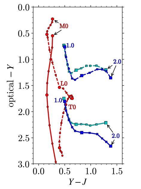
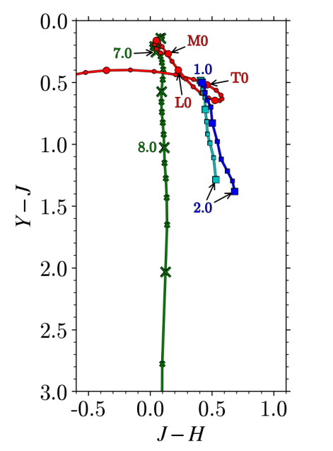
Figure 1: Model colour tracks of relevant populations. We describe the population modelling in Sect. 3.2. The separate populations are indicated as follows. The red tracks with circles show model MLT colours for each spectral type. The blue tracks with squares indicate early-type elliptical populations with two formation redshifts ($z_{\mathrm{f}}=3$, light blue; and $z_{\mathrm{f}}=10$, dark blue), with spacing $\Delta z=0.1$, and redshift labels. The green track with crosses indicates quasar model colours, with spacing $\Delta z=0.1$, and redshift labels. Upper: Optical-$YJ$ colours. $z>7$ quasars are expected to have negligible flux in both $O$ and $z$, so would appear below the bottom of the plot. We present separate tracks for the two optical bands. Solid lines indicate where the Euclid $O$ band is used in the optical. Dashed lines indicate where the ground-based $z$ band is used in the optical instead. Lower: Euclid $YJH$ colours.

The launch of Euclid, currently planned for Q2 2022, should prove to be a landmark in high-redshift quasar studies. An analysis of potential quasar yields in the Euclid wide survey was previously carried out for the Red Book (Laureijs et al., 2011, sect. 2.4.2), based on cuts in $YJH$ colour space. That report focused especially on $z>8.1$ quasars, which are much redder than the contaminants in $Y-J$, and so may be separated on that basis (see Laureijs et al. 2011, Figure 2.6). In contrast, over $7.2\lesssim z\lesssim 8.1$, near infrared broadband colours cannot easily separate quasars from contaminating populations, except with very deep complementary $z$-band data. Since then, the Euclid Near Infrared Spectrometer and Photometer (NISP) instrument wavelengths have changed (Maciaszek et al., 2016). In particular, this has resulted in bluer $Y-J$ colours for the three populations than was the case in Laureijs et al. (2011). We show the revised model colour tracks of the three populations that we consider in this work in Fig. 1.

Contamination becomes more of a problem at low S/N, which was dealt with in the Laureijs et al. (2011) analysis by selecting only bright point sources ($J_{\mathrm{AB}}<22$). Furthermore, it was argued that early-type galaxies at these brighter magnitudes might be identified and eliminated on the basis of their morphologies (we examine this assumption in more detail below). Assuming the $z=6$ QLF of Willott et al. (2010), with $k=-0.47$, it was predicted in Laureijs et al. (2011) that 30 $z>8.1$, $J_{\mathrm{AB}}<22$ quasars would be found in the $15\,000\,{\rm deg}^{2}$ wide survey.

Adopting the rate of decline $k=-0.72$ measured by Jiang et al. (2016), has a dramatic effect on the predicted numbers in Laureijs et al. (2011), reducing the yield of $z>8.1$ quasars from 30 to just eight. As already noted, the real situation may be worse than this, if the acceleration of the decline measured over $4<z<6$ continues beyond $z=6$. But if finding high-redshift quasars in Euclid will be more difficult than previously thought, this is true for all surveys, and the Euclid wide survey remains by far the best prospect for searches for high-redshift quasars. This motivates a deeper study of the problem, and reconsideration of the prospects for finding quasars in Euclid in the redshift interval $7<z<8$, as well as for finding fainter quasars ($J_{\mathrm{AB}}>22$) at $z>8$. The aim of this paper, therefore, is to improve on the Laureijs et al. (2011) analysis, and update predicted quasar numbers in the Euclid wide survey over the entire redshift interval $7<z<9$. To this end, we have developed better models of the contaminating populations, and we also explore more powerful selection methods which allow us to go fainter. We also consider the impact of deep ground-based $z$-band optical data on the predicted numbers.

The aim of this paper is to accurately model the high-redshift quasar selection process, and make robust predictions of the Euclid quasar yield, appropriate for the Euclid Reference Survey (ERS) currently defined in Scaramella et al. (in prep.). We compare selection using either Euclid or $z$-band optical data, focusing in particular on the overwhelming contamination from MLTs and early-type galaxies. The paper is structured as follows. We summarise the data that will be available to us, both from Euclid and from complementary ground-based surveys, in Sect. 2. We then describe the methods that we use to select $z>7$ quasars, and the population models that underpin them in Sect. 3. In Sect. 4 we present the results of simulations of high-redshift quasars, in the form of quasar selection functions, i.e., detection probabilities as a function of absolute magnitude and redshift, and the corresponding predicted numbers of quasars that will be discovered. In Sect. 5 we discuss the main uncertainties which will bear on the ability to select high-redshift quasars in the wide survey, and additionally discuss a potential timeline for Euclid $z>7$ quasar discoveries. We summarise in Sect. 6. We have adopted a flat cosmology with $h$ = 0.7, $\Omega_{\rm m}$ = 0.3, and $\Omega_{\Lambda}$ = 0.7. All magnitudes, colours and k-corrections quoted are on the AB system, and we drop the subscript for the remainder of the paper.

Table 1: Summary of survey combinations explored in simulations in this paper.

Survey(s)	Depth in near-infrared	Depth in optical	Positional constraints	Fiducial area
Euclid	$YJH$ 24.0 ($5\,\sigma$)	$O$ 24.5 ($10\,\sigma$)	ERS coverage (Fig. 2)	$15\,000\,{\rm deg}^{2}$
Euclid + PS (DR3)	$YJH$ 24.0 ($5\,\sigma$)	$z$ 24.5 ($5\,\sigma$)	as Euclid only, and $\delta>30$\mathrm{\SIUnitSymbolDegree}$$	$5\,000\,{\rm deg}^{2}$
Euclid + LSST (1 yr)	$YJH$ 24.0 ($5\,\sigma$)	$z$ 24.9 ($5\,\sigma$)	as Euclid only, and $\delta<30$\mathrm{\SIUnitSymbolDegree}$$	$10\,000\,{\rm deg}^{2}$

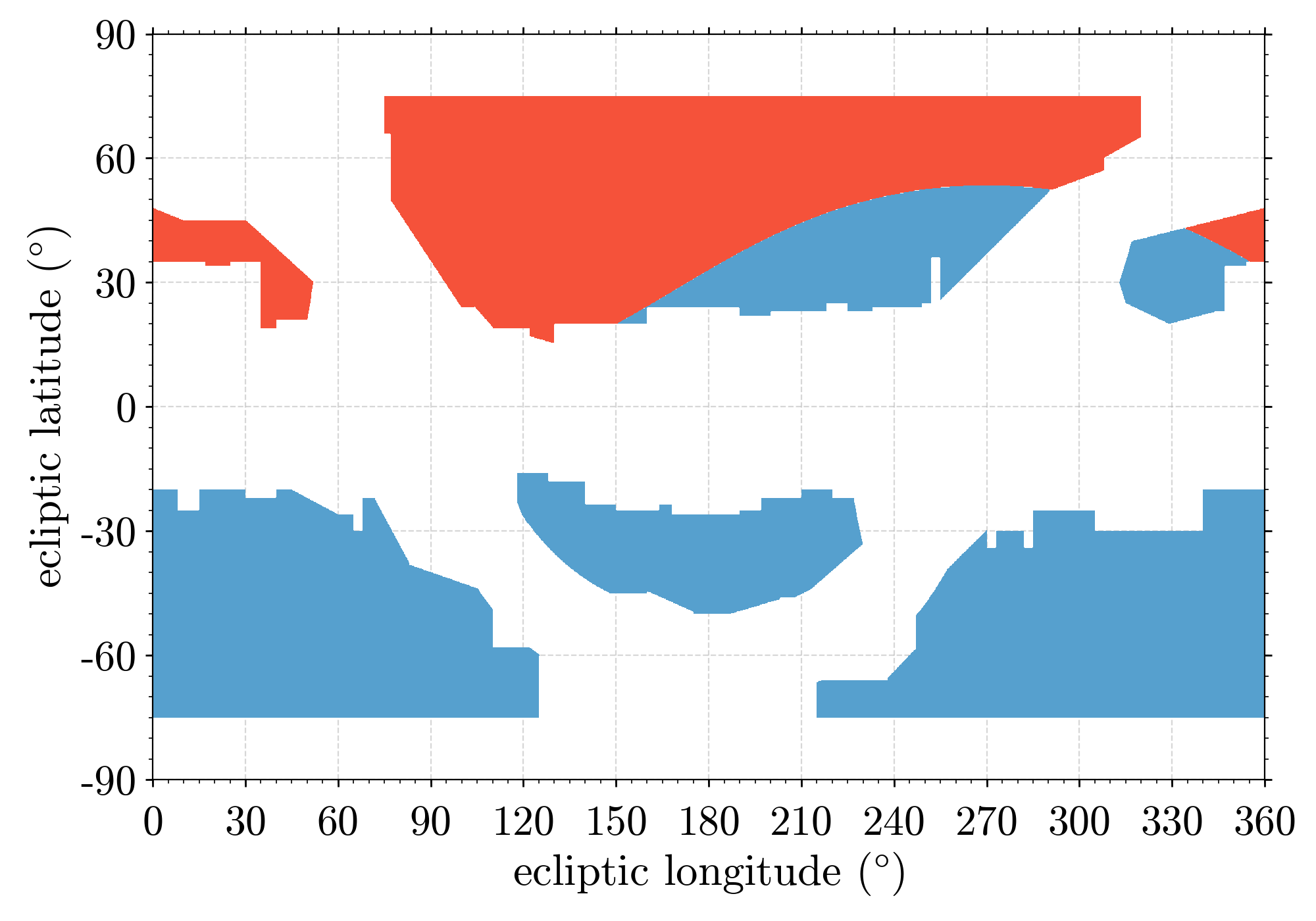
Figure 2: Cylindrical projection of the area from which we draw simulated quasars, in ecliptic coordinates, consistent with the ERS coverage defined in Scaramella et al. (in prep.). Euclid/Pan-STARRS sources are drawn from the red area with $\delta>30$\mathrm{\SIUnitSymbolDegree}$$, and Euclid/LSST sources from the blue area with $\delta<30$\mathrm{\SIUnitSymbolDegree}$$. The sample with no ground-based counterpart is drawn from the combined area.

2 Data

In Sect. 2.1 we give a brief technical overview of the Euclid wide survey (see Laureijs et al. 2011 and Scaramella et al., in prep., for further details). The search for high-redshift quasars is enhanced with deep data in the $z$ band, and we summarise complementary ground-based optical data in Sect. 2.2. The areas and depths of the Euclid and ground-based data are summarised in Table 1.

Since the ground-based data have not yet been secured, in this paper two scenarios are considered: i) the case where Euclid data are the only resource available, for which we consider optical data from the visual instrument, in a wide filter ($R+I+Z$) which for brevity we label $O$; and ii) where we replace Euclid optical data with complementary ground-based $z$-band data.

2.1 Euclid wide survey

The Euclid wide survey will offer an unprecedented resource for $z>7$ quasar searches, in terms of the combination of area covered and the NIR depths achieved. The six-year wide survey of Euclid will cover $15\,000\,{\rm deg}^{2}$ of extragalactic sky in four bands: a broad optical band ($O$; 5500 – 9000  Å); and three near-infrared bands, $Y$ (9650 – 11 920  Å), $J$ (11 920 – 15 440  Å) and $H$ (15 440 – 20 000  Å). The planned depths, from Laureijs et al. (2011), are provided in Table 1.

The exact sky coverage of the Euclid wide survey is yet to be finalised, with multiple possible solutions which satisfy the minimum area and science requirements laid out by Laureijs et al. (2011). The assumed sky coverage is relevant to this paper, because the surface density of MLT dwarfs depends on Galactic latitude (Sect. 3.2.2). To ensure the results of this paper accurately reflect quasar selection with Euclid, we follow the ERS shown in Scaramella et al. (in prep.), additionally indicated in Fig. 2. We assign random sky coordinates drawn from the wide survey to all sources that we simulate.

The fields are located at high Galactic latitudes, and so the reddening is low. It is estimated that reddening $E(B-V)$ exceeds 0.1 over only ${7}\,\textrm{--}\,{8}\%$ of the area (Galametz et al., 2017). Any small regions of significantly higher reddening will be excised from the search for quasars. For the remainder of the survey, with $E(B-V)<0.1$, the effect on the quasar search is very small. At this level of reddening the change in $Y-J$ colour of a quasar is 0.05. This degree of reddening is within the range of colour variation of normal quasars. The discrimination against MLT dwarfs and early-type galaxies will not be affected at this level of reddening since it is primarily set by the contrast at the Lyman break, which is barely changed.

The Euclid deep fields will ultimately reach two magnitudes fainter than the wide survey in OYJH; however, they are unlikely to prove such a useful resource for $z>7$ quasar searches, since they will cover a total area of just $40\,{\rm deg}^{2}$ (Scaramella et al. in prep.). Without any consideration of the completeness of a potential search for quasars in the deep survey, the Jiang et al. (2016) QLF ($k=-0.72$) implies 12 sources with $7<z<9$ in the magnitude range $J={24}\,\textrm{--}\,{26}$, i.e., in the deep survey but not the wide survey. As shown in Sect. 4.1, this is a factor of 10 – 20 lower than the predicted yield of $J\lesssim 23$ quasars from the wide survey, depending on the choice of optical data used to select candidates. Spectroscopic follow-up of $J>24$ quasar candidates in the deep fields will also prove challenging. Consequently, this work considers the Euclid wide survey only.

2.2 Ground-based $z$-band optical data

Sufficiently deep $z$-band data enhance the contrast provided across the Ly$\alpha$ break in quasar spectra, compared to the $O$ band (Fig. 1). At redshifts $z>7$, there is negligible flux blueward of the Ly$\alpha$ emission line in quasar spectra, meaning quasars appear below the bottom of the upper panel of Fig. 1. The $z-Y$ colours of the potential contaminating populations, MLTs, and early-type galaxies, are less red than for the quasars. The large width of the $O$ band softens the contrast between the colours of quasars and the colours of the contaminating populations.

We wish to evaluate the extent to which using deep complementary $z$-band data from LSST (Ivezić et al., 2008) and Pan-STARRS (Chambers et al., 2016) can improve quasar selection over $z={7}\,\textrm{--}\,{8}$. The current goal is that the entire wide survey area will be covered by a combination of Pan-STARRS in the northernmost $5000\,{\rm deg}^{2}$ of Euclid sky, with the remaining area covered by LSST (Rhodes et al., 2017). We therefore concentrate on these two ground-based resources.

The exact crossover areas between Euclid and the ground-based surveys, and the target $z$-band depths are still to be finalised, so we have made a set of working assumptions for the purposes of this paper, which are summarised in Table 1. We additionally indicate the assumed crossover area in Fig. 2. The adopted $5\,\sigma$ depth for LSST, $z=24.9$, is based on one year of data (following the start of operations scheduled for 2022), assuming 20 zenith observations of each source with a single-visit $5\,\sigma$ depth of $z=23.3$ (Ivezić et al., 2008). The proposed LSST crossover area is composed of three separate surveys: the LSST main survey covering $-62$\mathrm{\SIUnitSymbolDegree}$<\delta<2$\mathrm{\SIUnitSymbolDegree}$$, and northern ($2$\mathrm{\SIUnitSymbolDegree}$<\delta<30$\mathrm{\SIUnitSymbolDegree}$$) and southern ($-90$\mathrm{\SIUnitSymbolDegree}$<\delta<-62$\mathrm{\SIUnitSymbolDegree}$$) extensions, across which the final depths will differ (Rhodes et al., 2017); however, for the sake of simplicity, we assume a uniform LSST depth. For Pan-STARRS we assume the planned depth at the time of Euclid DR3 (2029), which is anticipated to be $z=24.5$ at ${\rm S/N}=5$. The Pan-STARRS and LSST $z$ filter curves are extremely similar, and the resulting $z-Y$ colours are essentially identical. Differences in the selection functions for the two surveys are driven by the different depths in $z$. Although not considered further here, we note the possibility of using $z$-band data from other sources in the future, e.g., DES, which will cover $5000\,{\rm deg}^{2}$ of sky, almost entirely in the southern celestial hemisphere, in common with LSST. DES is ultimately expected to reach a $5\,\sigma$ depth of $z\sim 24$ (e.g. Morganson et al., 2018), i.e., around 1 mag shallower than LSST; however, DES data will be available considerably sooner, with the final release (DR2) expected August 2020.

3 High-redshift quasar selection

In this work, predictions of quasar numbers from the Euclid wide survey are based on quasar selection functions, which reflect the sensitivity of Euclid to quasars using a particular selection method as a function of luminosity and redshift, and over which different QLFs can be integrated to determine quasar yields. The starting point is a large number of simulated quasars on a grid in luminosity/redshift space. We simulate realistic photometry for these sources using model colours (Sect. 3.2.1), and add Gaussian noise to the resulting fluxes based on the assumed depths in each band. We determine selection functions by recording the proportion recovered when given selection criteria are applied to the sample. For computing the selection function, the details of the completeness of the Euclid catalogues around the detection limit $J\sim 24$, are unimportant because we find the efficiency of the selection algorithm falls rapidly fainter than $J\sim 23$ (Sect. 4). As such we do not simulate the full Euclid detection process using the $Y+J+H$ stack, and require only that a source be measured with $J<24$ before we apply the selection criteria.

The analysis provided in Laureijs et al. (2011) was based on colour cuts, indicated in Fig. 1. This is an inefficient method as it does not weight the photometry in any way, and the chosen cuts are heuristic. Here, instead, we employ and compare two different statistical methods for selecting the quasars. These are described in Sect. 3.1. The first uses an update to the Bayesian model comparison (BMC) technique laid out by Mortlock et al. (2012). The second uses a simpler minimum-$\chi^{2}$ model fitting method (sometimes called ‘spectral energy distribution, or SED fitting’), very similar to the method of Reed et al. (2017). The methods are based on improved population models for the key contaminants: MLT dwarf types; and compact early-type galaxies. Both methods require model colours for each population. The BMC method additionally requires a model for the surface density of each source as a function of apparent magnitude. We present the population models in Sect. 3.2. In this work we assume that MLTs and early-type galaxies are the only relevant contaminating populations for the selection of high-redshift quasars in Euclid. In Sect. 5.4 we consider this assumption further, by analysing deep COSMOS data (Laigle et al., 2016). We do not see evidence for further populations that need be considered for high-redshift quasar searches with Euclid.

3.1 Selection methods

We will now describe the two methods which we use to select candidate high-redshift quasars. The BMC method is presented in Sect. 3.1.1, and the minimum-$\chi^{2}$ model fitting in Sect. 3.1.2. Both methods are based on linear fluxes and uncertainties in each photometric band, even where a source is too faint to be detected. As such, we require some form of list-driven photometry, i.e., forced aperture photometry in all bands, for all sources that satisfy given initial criteria.

3.1.1 Bayesian model comparison

The BMC method used in this work is principally the same as that proposed by Mortlock et al. (2012), which was used to discover the $z=7.08$ quasar ULAS J1120+0641. The crux of the method is to calculate a posterior quasar probability, $P_{\mathrm{q}}$, for each source in a given sample, which allows candidates to be selected and prioritised for follow-up. In short, $P_{\mathrm{q}}$ is given by the ratio of ‘weights’ ($W_{t}$) of each type of object $t$ under consideration. Mortlock et al. (2012) presented a general form for the calculation of $P_{\mathrm{q}}$ given any number of relevant populations, which in this case we take to be quasars, denoted $q$; MLTs, $s$; and early type galaxies, $g$. Explicitly, given a set of photometric data ${\bm{d}}$,

$$P_{\mathrm{q}}\equiv p\left(q\,\middle|\,\bm{d}\right)=\frac{W_{\mathrm{q}}\left(\bm{d}\right)}{W_{\mathrm{q}}\left(\bm{d}\right)+W_{\mathrm{s}}\left(\bm{d}\right)+W_{\mathrm{g}}\left(\bm{d}\right)}.$$ (2)

To calculate the individual weights for a population, $q$, $s$, or $g$, we simultaneously make use of all available photometric data for a source, combined with the surface density of the population, which serves as a prior. For any source, the weight of a particular population measures the relative probability that the source would have the particular measured fluxes, assuming it to be a member of that population, characterised by the model colours, and surface density as a function of apparent magnitude. Mortlock et al. (2012) applied the method to the case of two populations: quasars and M stars. Here we adopt the more general form of the method, and apply it to three populations, which we describe fully in Sect. 3.2. The MLT population itself is divided into a set of sub-populations, which are the individual spectral types from M0 to T8. This approach to the cool dwarf population is similar to that of Pipien et al. (2018), who developed models for each spectral type L0 – T9 in a search for high-redshift quasars in the Canada-France High-$z$ Quasar Survey in the Near-Infrared.

The individual weights for each population are calculated as follows:

$$W_{t}\left(\bm{d}\right)=\int\Sigma_{t}\left(\bm{\theta}_{t}\right)\;p\left(\bm{d}\,\middle|\,\bm{\theta}_{t},t\right)\;{\rm d}\bm{\theta}_{t},$$ (3)

where $\bm{\theta}_{t}$ is the set of parameters describing a single population. The two terms in the integral in Eq. (3) are respectively the surface density function, and a Gaussian likelihood function based on model colours, which is written in terms of linear fluxes. Explicitly, the full likelihood function is given by

$$p\left(\bm{d}\,\middle|\,\bm{\theta_{t}},t\right)=\prod_{b=1}^{N_{\mathrm{b}}}\,\frac{1}{\sqrt{2\pi}\,\hat{\sigma}_{b}}\,\exp\left\{-\frac{1}{2}\left[\frac{\hat{f}_{b}-f_{b}\left(\bm{\theta_{\emph{t}}}\right)}{\hat{\sigma}_{\emph{b}}}\right]^{2}\right\},$$ (4)

where the data in each of the $N_{\mathrm{b}}$ bands $b$ is of the form $\hat{f}_{b}\pm\hat{\sigma}_{b}$, and $f_{b}\left(\bm{\theta_{\emph{t}}}\right)$ is the true flux in band $b$ of an object of type $t$ described by the parameters $\bm{\theta_{t}}$. From the above definition of the individual population weights, which incorporates both the prior weighting and likelihood, it follows that the ratio of any pair of population probabilities ($P_{\mathrm{q}},P_{\mathrm{g}},P_{\mathrm{s}}$; cf. Eq. 2) yields the product of a prior ratio and a Bayes factor (e.g. Sivia & Skilling, 2006).

The chosen threshold value of $P_{\mathrm{q}}$ that defines the sample of candidate quasars, effects a balance between contamination and completeness. In this work the selection functions are computed for a probability threshold of $P_{\mathrm{q}}=0.1$, consistent with Mortlock et al. (2012). This implies a follow-up campaign to identify unambiguously all sources with $P_{\mathrm{q}}>0.1$, e.g., with spectroscopy. The value $P_{\mathrm{q}}=0.1$ was chosen initially because it worked well for the UKIDSS LAS high-redshift quasar survey (Mortlock et al., 2012). As a check we also carried out detailed simulations of the contaminating populations, i.e., we created a synthetic Euclid survey, and classified all sources. A small fraction of non-quasars are selected as quasars; however, $P_{\mathrm{q}}>0.1$ is sufficient to exclude the majority of contaminants. We present a full discussion of the Euclid contaminants in Sect. 4.3.

In practice, the $P_{\mathrm{q}}$ threshold will be set to control the number of candidates which are accepted for follow-up observation, based on the expected numbers of quasars, and will depend among other things on the reliability of the Euclid photometry, and the extent to which non-Gaussian errors (from whatever cause) afflict the data. A lower value of $P_{\mathrm{q}}$ can increase the quasar yield, at a cost of allowing greater contamination of the sample. In fact we find the selection functions, and therefore the predicted yield, are not particularly sensitive to the choice of threshold as typically quasars are recovered with high probability. Therefore, foreseeably, any $P_{\mathrm{q}}$ threshold in the range ${5}\,\textrm{--}\,{20}\%$ could be chosen, depending on the length of the actual candidate lists and the follow-up resources that are available.

3.1.2 $\chi^{2}$ model fitting

To assess the performance of the BMC method, we will also consider Euclid quasar selection using a minimum-$\chi^{2}$ technique. Such an approach has previously been used by, e.g., Reed et al. (2017), who discovered eight bright ($z_{\mathrm{AB}}<21.0$) $z\sim 6$ quasars, using a combination of DES, VHS and WISE data. We calculate $\chi^{2}_{\rm red}$ values for a given source and model SED $m$ as follows:

$$\chi^{2}_{{\rm red,}m}=\frac{1}{N_{\mathrm{b}}-2}\sum_{b}^{N_{\mathrm{b}}}\left(\frac{\hat{f}_{b}-s_{\rm best}\,f_{m,b}}{\hat{\sigma}_{b}}\right)^{2},$$ (5)

where $f_{m,b}$ is the (unnormalised) model SED flux in band $b$, and $s_{\rm best}$ is the normalisation that minimises $\chi^{2}$. We have $N_{\mathrm{b}}-2$ degrees of freedom as there are two parameters under consideration: the normalisation of a single model and the range of models being fitted (e.g. Skrzypek et al., 2015). (That is to say, for the quasars and early-type galaxies, the second parameter is redshift, while for the MLT dwarfs the second parameter is spectral type, since they form a continuous sequence.) The SED fitting can be linked to the BMC method by considering the logarithm of the likelihood given in Eq. (4). The key difference in the SED fitting method compared to the BMC method is that no surface density information is employed, i.e., we do not include a prior.

We use the model colours outlined in Sect. 3.2 to produce quasar and contaminant SEDs, and fit them to the fluxes of each source, following Eq. (5). Therefore for the MLTs each spectral type represents a model, while for the galaxies and quasars the set of models is defined by SEDs produced in intervals of $\Delta z=0.05$. We keep the single best fitting quasar $(q)$ model and contaminant $(c)$ model, with respective $\chi^{2}_{\rm red}$ values $\chi^{2}_{{\rm red,q(best)}}$ and $\chi^{2}_{{\rm red,c(best)}}$. Following Reed et al. (2017), we apply two cuts to the $\chi^{2}_{\rm red}$ values to retain a source (see Figure 15 of that work). We firstly require $\chi^{2}_{{\rm red,c(best)}}>10$, i.e., the data are a bad fit to all contaminant models. We additionally require the ratio $\chi^{2}_{{\rm red,c(best)}}/\chi^{2}_{{\rm red,q(best)}}>3$, i.e., the data are fit substantially better by a quasar SED than any contaminant model. In a similar way to the $P_{\mathrm{q}}$ threshold discussed in Sect. 3.1.1, these cuts do not have a particular statistical significance, but would be chosen to control future candidate lists. It is likely that the optimal thresholds for Euclid will ultimately differ from the Reed et al. (2017) study, due to differences in the data and the number of bands available, $N_{\mathrm{b}}$.

3.2 Population models

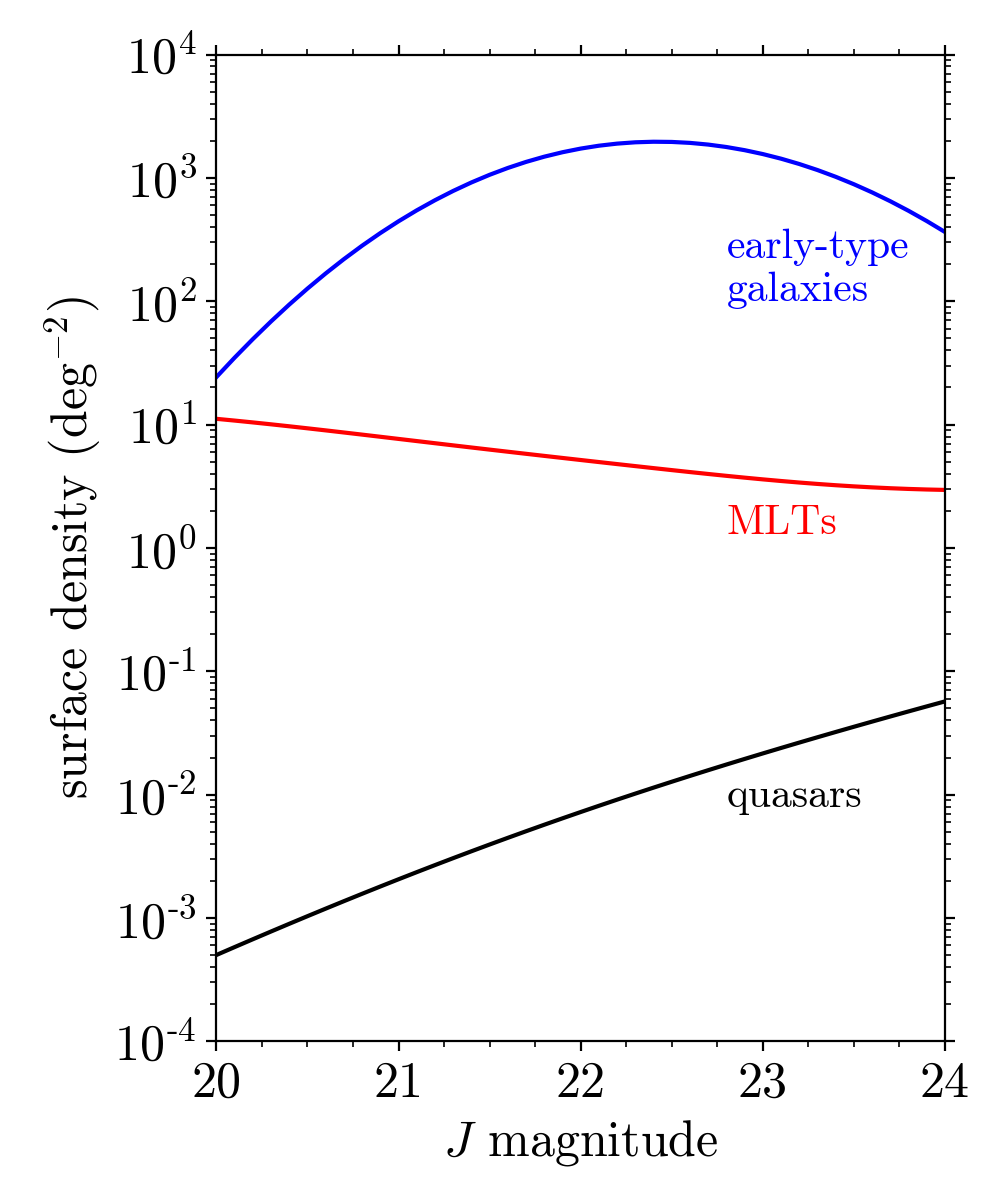
Figure 3: Population surface densities as a function of $J$-band magnitude. Blue: Early-type galaxies, integrated over the redshift range $z={1}\,\textrm{--}\,{2}$. Red: MLTs, summed over spectral type. Black: Quasars, integrated over over the redshift range $z={7}\,\textrm{--}\,{9}$.

We now summarise the surface density terms (Fig. 3) and model colours (shown in Fig. 1) which are used in the methods described in Sect. 3.1. We present the models for quasars in Sect. 3.2.1, for MLTs in Sect. 3.2.2, and for early-type galaxies in Sect. 3.2.3.

3.2.1 Quasars

The parameters $\bm{\theta}$ for the quasar weight $W_{\mathrm{q}}$ are absolute magnitude and redshift. The surface density term is based on the Jiang et al. (2016) QLF, extrapolated to redshifts $z>6$ assuming $k=-0.72$. We show the surface density of quasars in the redshift range $7.0\leq z\leq 9.0$ as a function of $J$ magnitude in Fig. 3. This helps to illustrate the difficulty associated with identifying quasars at $z>7$, as the quasar surface density is typically several orders of magnitude lower than those of both main contaminants.

Quasar k-corrections and colours, which are required for both selection methods, are measured directly from model spectra using synphot (Laidler et al., 2008). The model SEDs were determined using quasars with redshifts $0.1\leq z\leq 4.0$ from the SDSS DR7 (Schneider et al., 2010). Optical photometry from the SDSS was combined with near-infrared data from UKIDSS (Lawrence et al., 2007) and $W1$ and $W2$ photometry from WISE (Wright et al., 2010) to provide an extensive multi-wavelength data set. The quasar SED model was then generated via a minimisation procedure to determine parameter values for components including continuum power-law slopes, and emission-line equivalent widths. The model SED has seen extensive use (e.g. Hewett et al., 2006; Maddox et al., 2008, 2012), and reproduces the median photometric properties of the SDSS DR7 quasars to better than 5 per cent over the full redshift range $0.1\leq z\leq 4.0$.

In this paper we use a single reference model to represent typical quasars. This model is characterised by a set of emission line equivalent-width ratios. The standard line strength has rest frame equivalent width $\mathrm{EW_{{\rm C}\,\textsc{iv}}=39.1\,\AA}$ and UV continuum slope, defined by the ratio of $f_{\lambda}$ at rest frame $1315\,\AA$ and $2225\,\AA$, $f_{1315}/f_{2225}=1.0$. Since we are only interested in redshifts $z>7$, we assume that all flux blueward of Ly$\alpha$ is absorbed for all sources that we simulate, except that we include a near zone of size 3 Mpc (proper). The results are insensitive to the choice of near-zone size.

In the actual search of the Euclid data we will adopt a set of quasar spectral types, characterised by variations in the continuum (redder/bluer), and variations in the equivalent width of the reference C iv emission line, keeping all emission line ratios fixed. The surface density term (i.e., the prior) will be divided in proportion to the expected numbers, based on our knowledge of quasars at lower redshifts. The total quasar weight $W_{\mathrm{q}}$ is the sum of weights over the different types. This inference strategy is essential to maximise the yield from Euclid. The goal of the current paper, to compute the expected yield of high-redshift quasars, is different, and we can adopt a simpler strategy, and compute $W_{\mathrm{q}}$, and so $P_{\mathrm{q}}$, by adopting a single typical spectral type. Performing similar calculations for other surveys, the estimated yields are very similar for two scenarios: firstly, using a single spectral model for the simulated population of quasars, and the same model (i.e., colour track) for the selection algorithm; secondly, using a range of quasar models, suitably weighted, for the simulated quasars, and using the same range of models, and weights, in the selection algorithm. This statement is only true if the single model adopted is typical, i.e., of average line width and continuum slope. The reason for this is that objects with, e.g., stronger (weaker) lines have a higher (lower) probability of selection, compared to the typical spectrum, and the corresponding gains and deficits approximately cancel. Therefore a selection function weighted over the different spectral types is very similar to the selection function computed for the average type. In addition, the computation of selection functions is considerably faster when a single SED is used, since one value of $W_{\mathrm{q}}$ is calculated for a single grid of simulated quasars (around 500,000 objects). Extending the problem to $n$ SEDs requires the calculation of $n$ individual quasar weights, for $n$ grids of quasars of different types. We consider this matter further in Sect. 5.6 where we investigate templates with different continuum slopes and line strengths. The analysis therein reinforces the above conclusion.

Irrespective of the intrinsic quasar SEDs adopted, neutral hydrogen along the line of sight will mean they have no significant flux in bands blueward of the redshifted Ly$\alpha$ line, and so all standard search methods exploit the fact that they will be optical drop-out sources. This approach, however, ignores the possibility of gravitational lensing by an intervening galaxy that both magnifies the quasar image(s) and directly contributes optical flux. There have been theoretical predictions that the fraction of multiply imaged quasars in a flux-limited sample could be up to  30% (Wyithe & Loeb, 2002), although empirically this fraction is closer to 1% (Fan et al., 2019). It has been argued (Fan et al., 2019; Pacucci & Loeb, 2019) that this discrepancy is because the optical flux from the deflector galaxies mean that lensed high-redshift sources are not optical drop-outs. If this is the dominant effect then there would be an additional population of $z>7$ quasars beyond that considered here. However, whether they would be detectable depends on the numbers of contaminating sources with comparable optical-NIR colours, which we do not explore in this work.

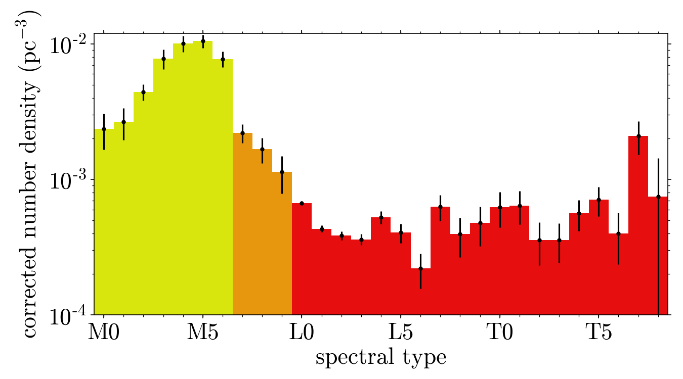
Figure 4: MLT number densities at the Galactic central plane. M0 – M6 (yellow) are determined from the Bochanski et al. (2010) luminosity function. M7 – M9 (orange) are extrapolated from L0, satisfying the Cruz et al. (2007) measurement. We measure L0 – T8 (red) number densities from the Skrzypek et al. (2016) LAS sample.

Table 2: MLT density at the Galactic plane, and model colour data. $z-Y$ is applicable to both LSST and Pan-STARRS. We additionally show the MLT colours in Fig. 1.

SpT $\rho_{0}\leavevmode\nobreak\ (\mathrm{pc^{-3}})$ $M_{J}$ $z-Y$ $O-Y$ $Y-J$ $\leavevmode\nobreak\ J-H$ M0 $2.4\times 10^{-3}$ 6.49 0.23 0.55 0.27 $0.15$ M1 $2.7\times 10^{-3}$ 7.07 0.29 0.78 0.26 $0.08$ M2 $4.4\times 10^{-3}$ 7.71 0.35 1.00 0.23 $0.05$ M3 $7.8\times 10^{-3}$ 8.28 0.41 1.23 0.19 $0.04$ M4 $1.0\times 10^{-2}$ 8.90 0.46 1.46 0.17 $0.04$ M5 $1.1\times 10^{-2}$ 9.53 0.52 1.68 0.16 $0.05$ M6 $7.8\times 10^{-3}$ 10.85 0.58 1.91 0.18 $0.07$ M7 $2.2\times 10^{-3}$ 11.66 0.82 2.26 0.21 $0.10$ M8 $1.7\times 10^{-3}$ 12.08 1.06 2.61 0.26 $0.13$ M9 $1.1\times 10^{-3}$ 12.33 1.30 2.96 0.33 $0.18$ L0 $6.7\times 10^{-4}$ 12.54 1.54 3.32 0.40 $0.23$ L1 $4.3\times 10^{-4}$ 12.79 1.56 3.32 0.47 $0.29$ L2 $3.8\times 10^{-4}$ 13.11 1.64 3.42 0.54 $0.35$ L3 $3.6\times 10^{-4}$ 13.50 1.72 3.51 0.59 $0.41$ L4 $5.3\times 10^{-4}$ 13.93 1.75 3.56 0.63 $0.47$ L5 $4.1\times 10^{-4}$ 14.38 1.75 3.55 0.65 $0.52$ L6 $2.2\times 10^{-4}$ 14.80 1.72 3.53 0.65 $0.56$ L7 $6.3\times 10^{-4}$ 15.17 1.69 3.51 0.63 $0.58$ L8 $3.9\times 10^{-4}$ 15.44 1.70 3.54 0.60 $0.57$ L9 $4.8\times 10^{-4}$ 15.63 1.76 3.63 0.56 $0.53$ T0 $6.3\times 10^{-4}$ 15.72 1.87 3.79 0.52 $0.46$ T1 $6.4\times 10^{-4}$ 15.74 2.03 4.00 0.48 $0.35$ T2 $3.6\times 10^{-4}$ 15.71 2.22 4.24 0.44 $0.21$ T3 $3.6\times 10^{-4}$ 15.69 2.41 4.47 0.41 $0.03$ T4 $5.6\times 10^{-4}$ 15.74 2.58 4.64 0.40 $-0.16$ T5 $7.1\times 10^{-4}$ 15.93 2.69 4.73 0.40 $-0.36$ T6 $4.0\times 10^{-4}$ 16.32 2.75 4.73 0.42 $-0.52$ T7 $2.1\times 10^{-3}$ 16.98 2.78 4.72 0.44 $-0.64$ T8 $7.5\times 10^{-4}$ 17.95 2.84 4.80 0.46 $-0.65$

3.2.2 MLT dwarfs

Most MLT dwarfs detected in the Euclid wide survey will be members of the Galactic thin disk. At the end of this section we also consider the possibility that members of the thick disk (larger scale height, lower metallicity) need to be considered as potential contaminants. The number density of the thin disk population is assumed to vary as $\rho=\rho_{0}\,e^{-Z/Z_{\mathrm{s}}}$, where $\rho_{0}$ is the number density of any spectral type M0 – T8 at the Galactic central plane, $Z$ is the vertical distance from the plane, and $Z_{\mathrm{s}}$ is the scale height, assumed to be 300 pc (e.g. Gilmore & Reid, 1983). The small offset of the Sun from the Galactic central plane is ignored. Each spectral type, or sub-population, is then specified by the value of $\rho_{0}$, the absolute magnitude in the $J$ band, and the $zOYJH$ colours. The values adopted are provided in Table 2. In determining $W_{\mathrm{s}}$, weights are computed for each spectral type, with the total weight $W_{\mathrm{s}}$ given by a sum over types. In this work, random coordinates are drawn from the Euclid wide survey (Sect. 2.1) for each simulated source, allowing us to fully incorporate Galactic latitude in the calculation of $W_{\mathrm{s}}$. In the case of simulated MLTs (Sect. 4.3), the coordinates that are drawn additionally preserve the dependence on Galactic latitude.

We assigned colours for each spectral type by measuring colours for suitable sources in the SpeX Prism Library (Burgasser, 2014), and selecting the median value for each spectral type. Holwerda et al. (2018) recently presented Euclid NIR colours for the MLT population. They took a different approach, by measuring colours for the standard stars in the library; however, these individual spectra do not extend sufficiently bluewards to measure optical colours. In addition to the colours presented in Table 2, we determine median SDSS $riz$ colours for types M0 – M6, using bright sources from the West et al. (2011) sample. These colours are required to compute number densities and absolute magnitudes as detailed below.

Number densities for types M0 – M6 are based on the luminosity function of Bochanski et al. (2010) as follows. Interpolating the model $i-z$ colours, we approximate a range in $i-z$ for each spectral type using the range $\left[\mathrm{SpT}-0.5,\mathrm{SpT}+0.5\right]$. The $i-z$ colour evolves linearly over the early M types, and we simply extrapolate to K9 to determine the $i-z$ range for M0. The M7 $i-z$ colour, needed to define the M6 range, comes from Skrzypek et al. (2016). Using the relation in Bochanski et al. (2010), we convert the $i-z$ range for each spectral type into a range in $M_{r}$. The last step is to interpolate the binned system luminosity function in Bochanski et al. (2010). Integrating over the $M_{r}$ range for each spectral type, we finally obtain number densities in ${\rm pc^{-3}}$.

The L- and T-type number densities were calculated using the UKIDSS LAS LT sample presented by Skrzypek et al. (2016). For a particular spectral type, we computed the value of $\rho_{0}$ that reproduces the number of sources in the sample, given the assumed scale height, the magnitude range of the sample, and the solid angle of the survey as a function of Galactic latitude. For M7 – M9 we use Cruz et al. (2007), who measure a total number density of $4.9\times 10^{-3}\,{\rm pc^{-3}}$ for these three spectral types. We approximate the individual number densities by assuming the number density varies linearly across the range M7 – L0, constrained such that the total Cruz et al. (2007) number density is reproduced. The number density as a function of spectral type is ploted in Fig. 4, while the surface density summed over spectral types is shown as a function of $J$ magnitude in Fig. 3. Dupuy & Liu (2012) provide $J$-band absolute magnitudes for spectral types M6 – T8. For M0 – M5 we use Bochanski et al. (2010) to determine $r$-band absolute magnitudes, again based on the $i-z$ colour for each spectral type, and use model colours to convert $M_{r}$ to $M_{J}$.

Euclid is sufficiently deep that we expect the metal-poor MLT population of the thick disk, i.e., ultracool subdwarfs (Zhang et al., 2018), to become important at faint magnitudes. Assuming that the thick disk population contributes 10% of the stellar number density at the Milky Way central plane, and has a scale height of 700 pc (Ferguson et al., 2017), the expected number densities of thin and thick disk stars become comparable at vertical distances $\sim 1200$ pc from the Galactic plane, meaning that the thick disk dwarfs need to be considered in addition to the thin disk dwarfs. The luminosities in Table 2 imply spectral types down to L3 will be observable with $J<24$ at such distances, and so may become a comparable source of contamination at faint Euclid magnitudes. However, in Sect. 4.3 we find the most important spectral types in terms of contamination are in the range T2 – T4. These types are only observable to distances of $\sim 450$ pc with $J<24$, meaning the equivalent subdwarfs are unlikely to be a significant source of contamination. Additionally, the subdwarf population is bluer than MLTs in the thin disk, which will help with discrimination from quasars. This was determined using the L subdwarfs presented by Zhang et al. (2018). For objects in Table 1 of that work that matched to the UKIDSS LAS, we measured the UKIDSS $Y-J$ colours and compared against the template colours from Skrzypek et al. (2015) for each spectral type. We found L type subdwarfs are on average 0.24 mag bluer in $Y-J$ than the corresponding L dwarfs, meaning that contamination by subdwarfs is much less of a concern. For these reasons we do not include the thick disk in our modelling of MLTs.

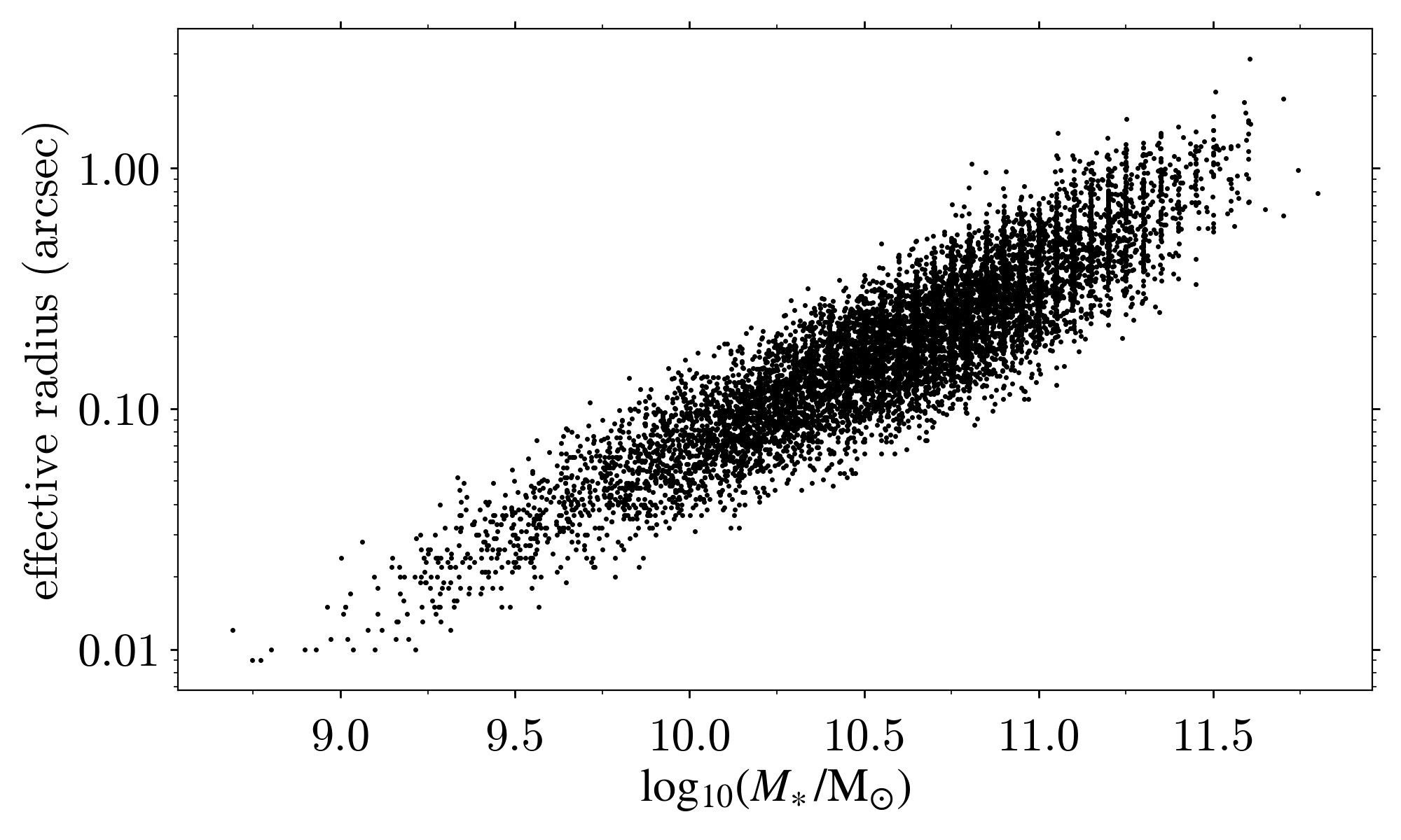
Figure 5: Distribution of sizes of quiescent COSMOS galaxies as a function of $M_{*}$, based on the relation and scatter measured by van der Wel et al. (2014).

3.2.3 Early-type galaxies

Early-type galaxies over the redshift range $z={1}\,\textrm{--}\,{2}$ have very red $zOYJH$ colours, that resemble the colours of high-redshift quasars at low S/N. There is a steep correlation between size and stellar mass for this population (van der Wel et al., 2014). As a consequence, faint $J>22$ early-type galaxies at these redshifts will be very compact. The $0.\mathrm{″}3$ pixel size of the Euclid NISP instrument means that the surface brightness profiles of these faint early type galaxies will be poorly sampled, and therefore they may be mistaken for point sources, and classified as quasars. We now consider this possibility. While the pixel size of the Euclid VIS instrument, $0.\mathrm{″}1$, is much better, the detection S/N in the $O$ band will be very low, e.g., for a $J=23$ early-type galaxy observed at $z=1.5$, the model $O-J$ colour (described below) is greater than 2.5, implying $\left({\rm S/N}\right)_{O}<5$.

The best sample for investigating this issue, i.e., from the survey with the largest available area and that is deep enough for the Euclid analysis, is the COSMOS sample presented by Laigle et al. (2016). There is a total of $1.38\,{\rm deg}^{2}$ of crossover between COSMOS, and the NIR UltraVISTA bands. We use only the quiescent objects from Laigle et al. (2016), which are selected on the basis of a rest frame NUV/optical optical/NIR colour cut, and we limit the analysis to redshifts $z={1}\,\textrm{--}\,{2}$. We additionally impose a magnitude cut, requiring $J<24$, which is sufficiently faint for the Euclid wide survey. (The quoted $2$\mathrm{\SIUnitSymbolArcsecond}$,3\,\sigma$ COSMOS depth is $J=25.2$, so incompleteness at $J<24$ will be negligible.)

All the COSMOS sources have a measured total $J$ magnitude, an estimate of the total stellar mass ($M_{*}$), and a photometric redshift. To establish the distribution of sizes, we use the relations between effective radius (of the assumed de Vaucouleurs $r^{1/4}$ profile) and stellar mass for quiescent galaxies, in different redshift bins, presented by van der Wel et al. (2014). For a COSMOS galaxy with a particular stellar mass and redshift, we draw a random size from the distribution, given the specified variance. The resulting distribution of sizes of the COSMOS sample is plotted as a function of $M_{*}$ in Fig. 5. Because we have a total magnitude for each source, we now have a sample that represents the complete magnitude/size/redshift distribution of the population at $1<z<2$.

At this point, ideally, we would simulate the detection, classification (star/galaxy discrimination), and photometry processes of the Euclid pipeline on this sample, to derive the surface density of the population of early-type galaxies with $1<z<2$, classified as point sources, as a function of point-source magnitude and redshift. This detailed modelling has not yet been undertaken. Therefore to make progress, we start with the simplifying assumption that aperture photometry in a $1.\mathrm{″}0$ aperture provides a reasonable approximation of the Euclid point-source photometry, recalling the large pixel size of the NISP instrument.

For each source in the COSMOS sample, we have integrated the $r^{1/4}$ profiles to correct the total magnitudes to this aperture size. The resulting $1\mathrm{″}$ $J$-band magnitudes (denoted $J_{1}$) are plotted as a function of effective radius in Fig. 6. The question now is what fraction of these galaxies would be classified as point sources? Using the BMC algorithm (for any sensible prior), we find that brighter than aperture magnitude $J_{1}=22$, the S/N is sufficiently high that quasars are cleanly discriminated from galaxies on the basis of their colours (Sect. 4). The question of point/extended source discrimination is therefore immaterial at these brighter magnitudes. Fainter than $J_{1}=22$ the colour discrimination begins to fall below $100\%$ success, i.e., some quasars do not satisfy the selection threshold, and are misclassified. Consequently we focus now on these fainter magnitudes.

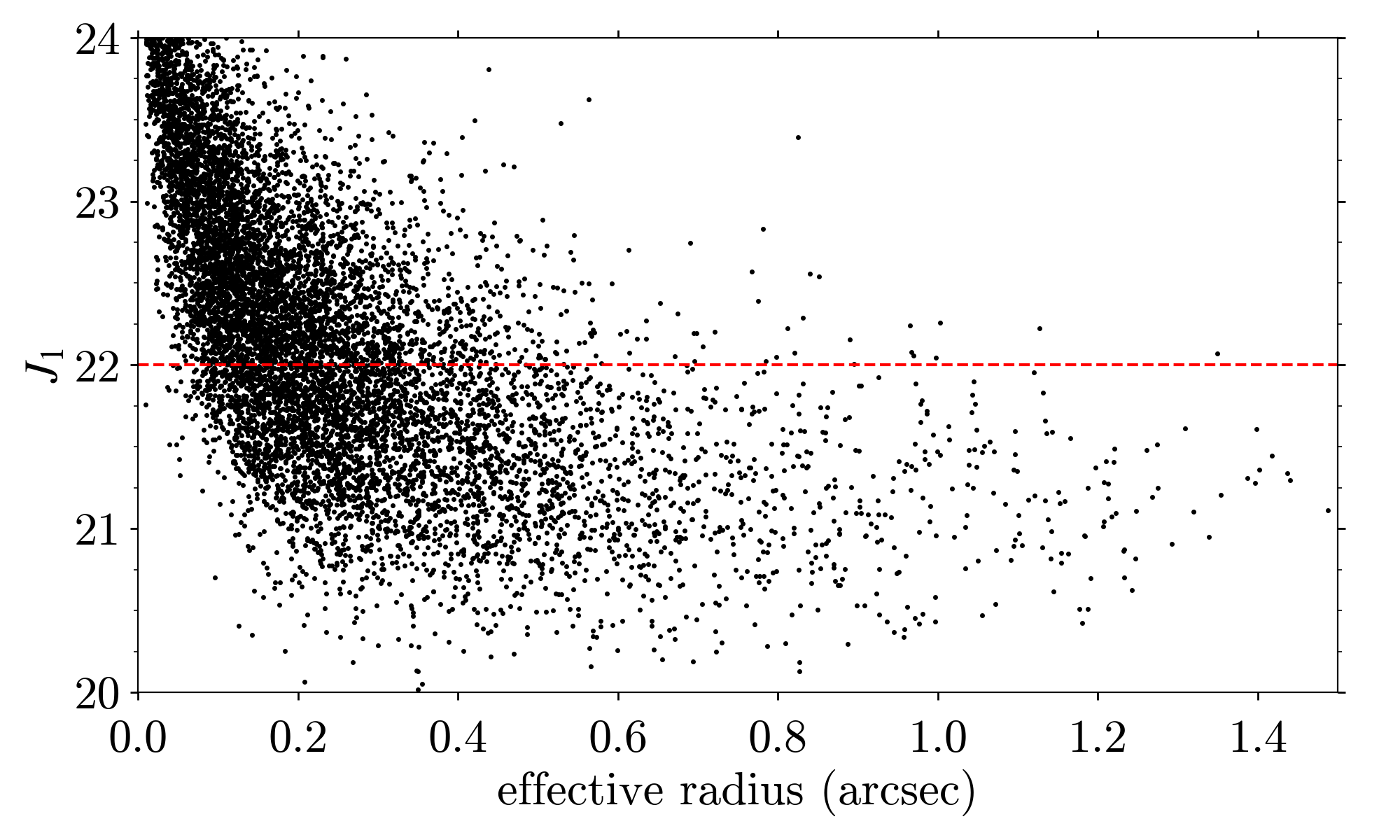
Figure 6: $1\mathrm{″}$ $J$-band aperture magnitude of COSMOS galaxies, as a function of half-light radius (see Fig. 5). Magnitudes fainter than $J=22$, above the red dashed line, are of particular relevance due to their predicted small radii.

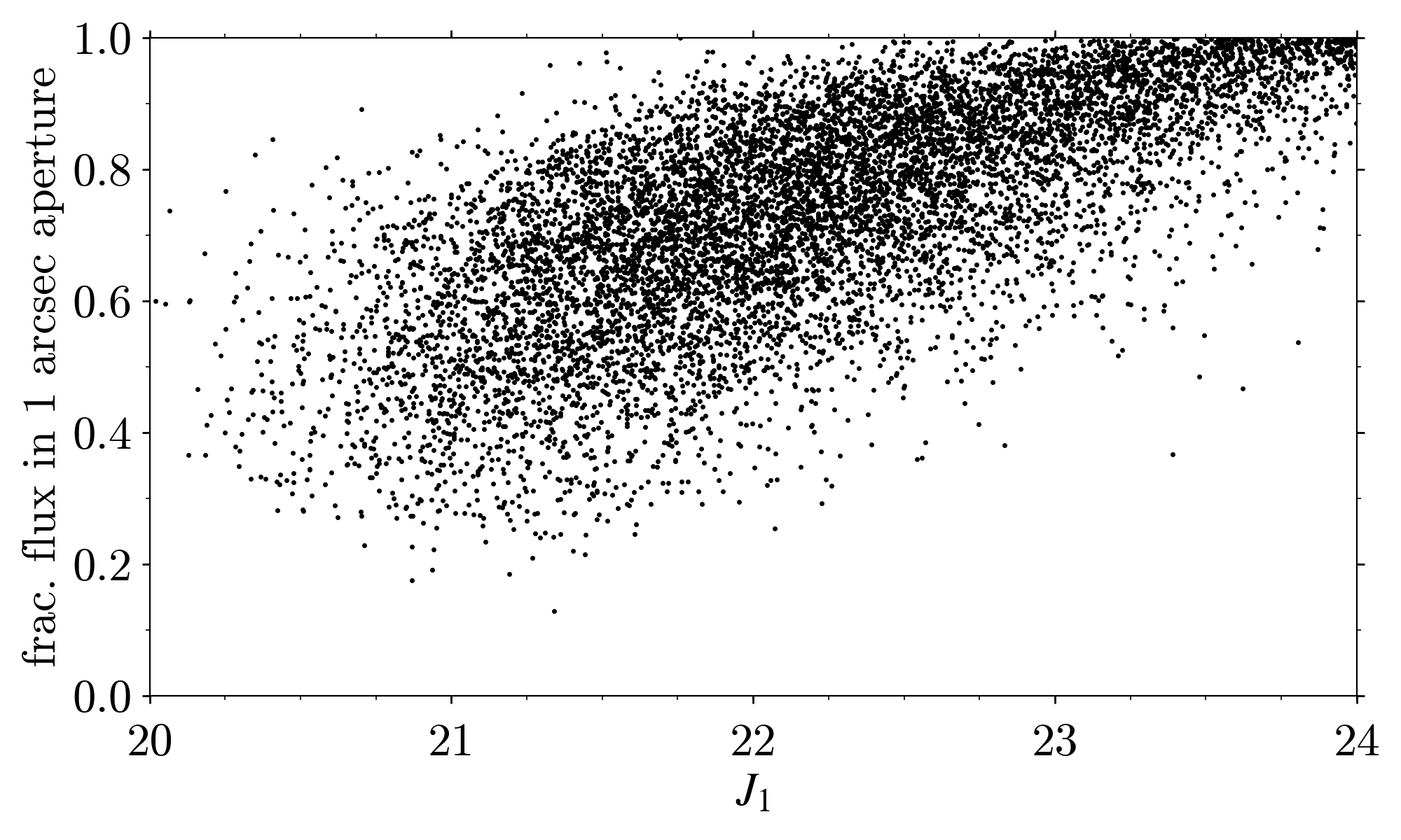
Figure 7: The fraction of flux contained in a $1\mathrm{″}$ diameter aperture, against $1\mathrm{″}$ $J$-band magnitude, measured for the COSMOS sample. The flux fractions are determined by integrating de Vaucouleurs profiles.

As can be seen from Fig. 6, fainter than $J_{1}=22$ the galaxies are very compact, with effective radii mostly less than $0.\mathrm{″}2$, meaning that many galaxies may be classified as point sources. Another way of seeing the problem is illustrated in Fig. 7 which plots the fraction of the total flux inside the $1\mathrm{″}$ diameter aperture. At $J_{1}=22$, the aperture contains on average $\sim 70\%$ of the total flux, increasing to $\sim 90\%$ at $J_{1}=23$. It is likely that most of these fainter galaxies, detected in $J$ at ${\rm S/N}\sim 10$, will be classified as point sources. For the purposes of this paper, we take a conservative approach and assume that all $J_{1}>22$ early-type galaxies $1<z<2$ will be classified as point sources by Euclid. We examine the consequences of this choice in Sect. 5.

To model the colours, we estimate formation redshifts ($z_{\mathrm{f}}$) by combining redshift and age data provided by Laigle et al. (2016). The histogram of $z_{\mathrm{f}}$ shows a peak near $z_{\mathrm{f}}=3$, with an extended tail towards higher redshifts. Consequently, we approximate the catalogue as two populations with a fraction 0.8 with $z_{\mathrm{f}}=3$, and a fraction 0.2 with $z_{\mathrm{f}}=10$, to try and encapsulate the range of formation redshifts seen in the data. We compute colours for both formation redshifts from the evolutionary models of Bruzual & Charlot (2003). The models are computed using the Chabrier (2003) initial mass function and stellar evolutionary tracks prescribed by Padova 1994 (e.g. Girardi et al., 1996). We use single stellar populations with solar metallicity (M62; $Z=0.02$) at our chosen formation redshifts and evolve them in time steps corresponding to $\delta z=0.1$ to cover the redshift range $1.0\leq z\leq 2.0$.

The galaxy surface density function is determined from a maximum likelihood fit to the COSMOS data, in terms of $J_{1}$ and source redshift. The functional form of the galaxy surface density function in units of $\mathrm{mag}^{-1}\,\mathrm{deg}^{-2}$ per unit redshift is

$$\Sigma(J_{1},z)=\alpha\,\exp\left\{-\frac{1}{2}\left[\frac{J_{1}-f\left(z\right)}{\sigma}\right]^{2}\right\}\,\exp\left[-\left(\frac{z-0.8}{z_{0}}\right)\right]$$ (6)

$$f\left(z\right)=J_{0}+b\,z,$$

where we find the best-fitting parameters to be $\left(\alpha,\sigma,J_{0},b,z_{0}\right)=\left(8969,0.770,20.692,1.332,0.424\right)$. We show this surface density function integrated over $1.0\leq z\leq 2.0$ as a function of $J$ magnitude in Fig. 3. We assume the same function is applicable to early-type galaxies with either formation redshift, and scale the resulting weights by 0.8 for $z_{\mathrm{f}}=3$ and 0.2 for $z_{\mathrm{f}}=10$ to reflect the distribution of $z_{\mathrm{f}}$ values seen in the COSMOS data.

Contamination from faint early-type galaxies may ultimately prove to be less important for $z>7$ quasar searches than presented in this paper. It may prove possible to increase the image sampling in NISP, by drizzling multiple exposures of the same field, which will improve star/galaxy discrimination, and hence reduce the number of contaminants. Whether or not these objects will actually be classified as point sources could be determined by including the population in future generations of Euclid simulations. Even if the effective radii of the galaxies are $0.\mathrm{″}2$ or smaller, it may be possible to identify light extending outside this radius if the PSF is well understood (e.g. Trujillo et al., 2006). Additionally, we have been somewhat conservative in assuming a minimum formation redshift of $z=3$, and a single burst of star formation. The COSMOS sample includes galaxies with later formation redshifts, which may also have some ongoing star formation, rendering them more visible in the $O$ band (Conselice et al., 2011).

4 Results

To model Euclid selection of high-redshift quasars, we apply the BMC and minimum-$\chi^{2}$ model fitting methods outlined in Sect. 3.1 to the simulated quasar grids. The main results are selection functions (Figs. 8 and 10), which we combine with population models to obtain predicted numbers (Table 3). In Sect. 4.1 we discuss the results from the BMC technique, and consider the impact of ground-based optical data. In Sect. 4.2 we compare against the $\chi^{2}$ method. In Sect. 4.3 we consider the extent of contamination by MLTs and ellipticals which are selected as quasar candidates.

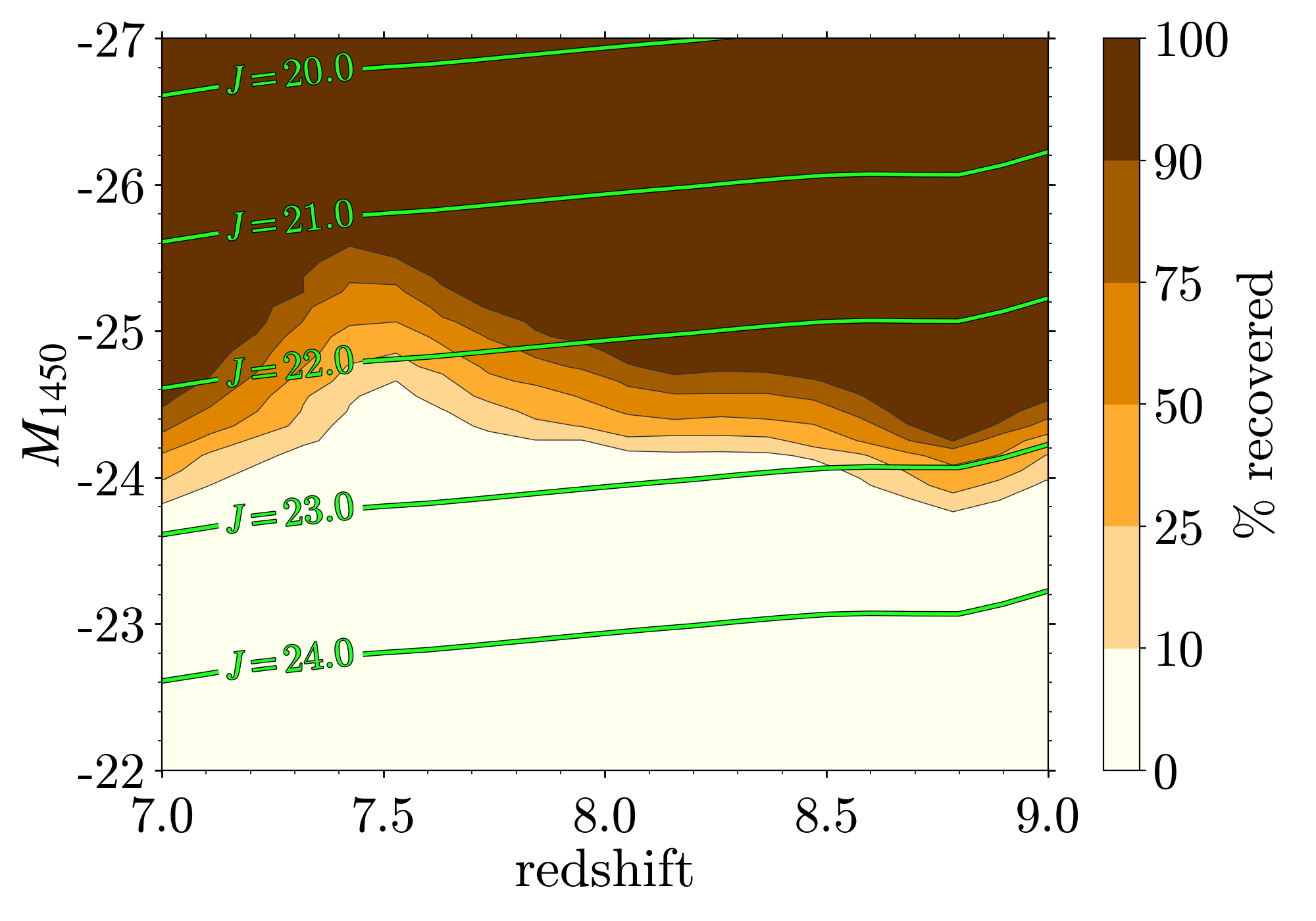
(a) Euclid data only.

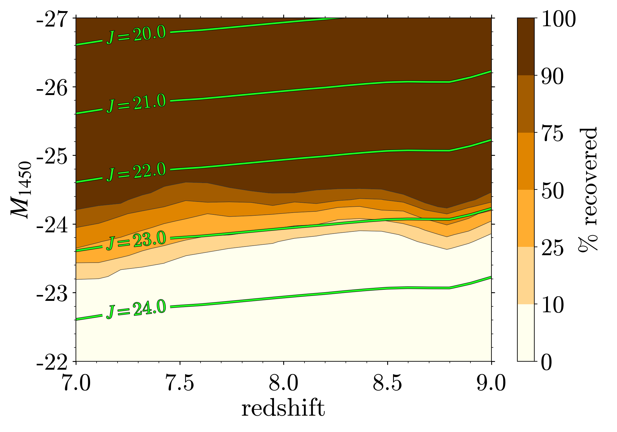
(b) Euclid $O$ band replaced with ground-based optical data.

Figure 8: Quasar selection functions determined using the BMC method for Euclid $YJH$ data with a) Euclid optical data, b) ground-based optical data. A quasar is defined as selected if $P_{\mathrm{q}}>0.1$. Contours of apparent magnitude are indicated by the labelled green lines.

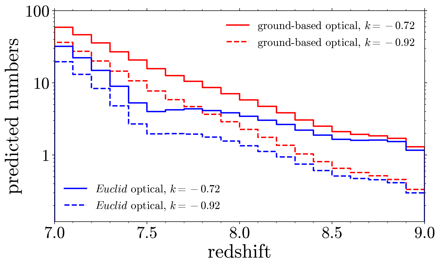
(a) Predicted yield in redshift bins of $\Delta z=0.1$.

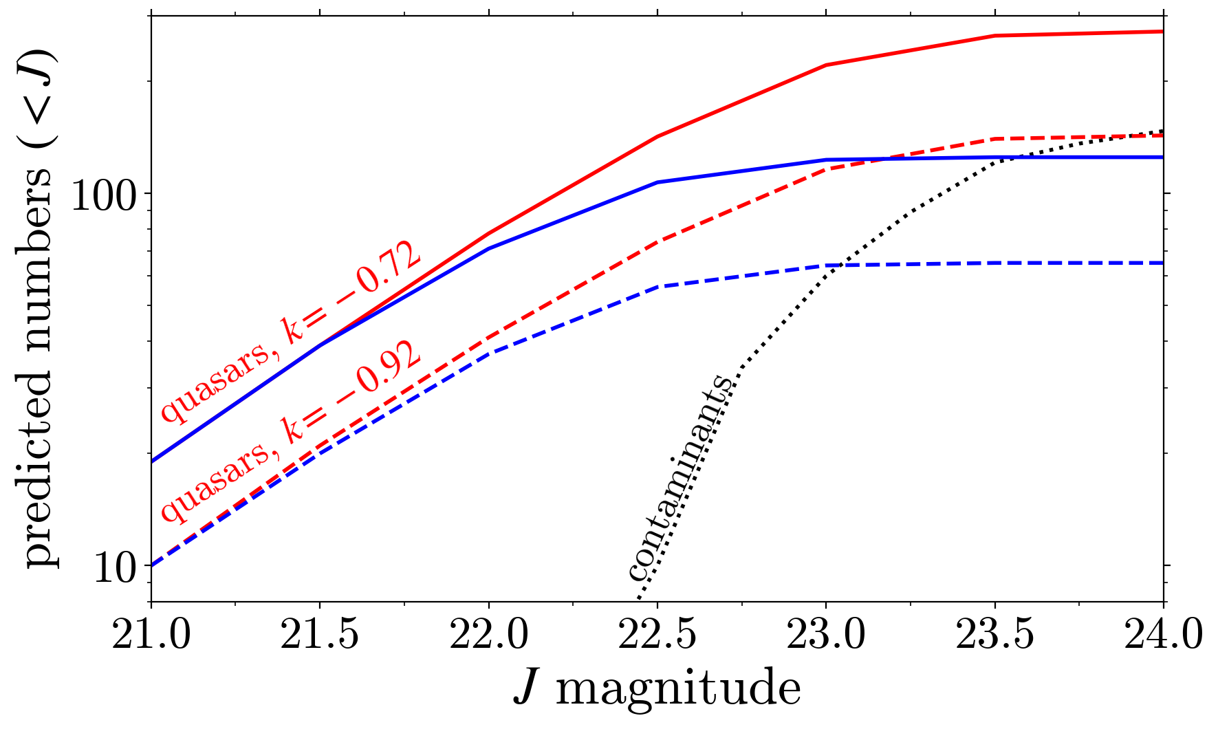
(b) Cumulative predicted yield as a function of $J$ magnitude.

Figure 9: Predicted numbers of $7<z<9$ quasars as a function of redshift (left) and $J$ magnitude (right), determined by integrating the QLF over the selection functions presented in Fig. 8, and assuming an area of $15\,000\,{\rm deg}^{2}$. Blue: Euclid data only. Red: Euclid $O$ band replaced with ground-based optical data. Solid lines $k=-0.72$. Dashed lines $k=-0.92$. The additional black dotted curve on the right-hand panel indicates the estimated number of contaminants selected as quasar candidates as a function of magnitude, assuming ground-based optical data, and so should be compared to the red curves, labelled.

Table 3: Summary of predicted numbers of Euclid wide survey quasars in redshift bins, determined by integrating the QLF over the BMC and minimum-$\chi^{2}$ quasar selection functions. Results are presented incorporating either Euclid or ground-based optical data, for two redshift evolutions of the QLF. Numbers from the minimum-$\chi^{2}$ model fitting are additionally given in brackets.

Redshift range Euclid optical Ground-based optical $k=-0.72$ $k=-0.92$ $k=-0.72$ $k=-0.92$ $7.0<z<7.5$ 87 (41) 51 (24) 204 (91) 117 (52) $7.5<z<8.0$ 20 (13) 9 (6) 45 (26) 19 (11) $8.0<z<8.5$ 11 (11) 4 (4) 16 (14) 6 (5) $8.5<z<9.0$ 6 (6) 2 (2) 7 (7) 2 (2)

4.1 Bayesian model comparison

We present the quasar selection function determined with the BMC technique, and using Euclid optical data, in Fig. 8a. This shows that over the redshift range $8<z<9$, quasars may be selected fainter than the previously assumed limit of $J=22$. The situation is worse over the redshift range $7<z<8$, where the discrimination against MLT dwarfs is relatively poor, and the typical depth reached is $J\sim 22$.

The selection function for the case where deep ground-based $z$-band data are available is presented in Fig. 8b. There is only a small difference between the individual LSST and Pan-STARRS selection functions, driven by the different depths of the surveys. For simplicity, we combine the LSST and Pan-STARRS selection functions in the ratio 2:1 (to reflect the respective areas), and present a single ‘ground-based’ selection function. As can be seen, the use of $z$-band optical data, compared to Euclid $O$-band data, means the quasar survey can reach up to 1 mag deeper over the redshift range $7<z<8$. There is also improvement over the redshift range $8<z<8.5$, while between $8.5<z<9$ the improvement is smaller. Broadly speaking, we now recover quasars as faint as $J\sim 23$ over the full redshift range $7<z<9$.

At redshifts $7<z<8$ the survey depth is set by the ability to discriminate against MLT dwarfs. Over the redshift range $8<z<9$ the contaminant weights are more balanced, i.e., the quasars that are not recovered are misclassified either as early-type galaxies or MLTs. In Sect. 5 we discuss the individual impact of the two contaminating populations on the quasar selection functions.

To estimate the number of quasars that can be detected in the Euclid wide survey, we integrate two different QLFs over the selection functions We adopt the Jiang et al. (2016) $z=6$ QLF, with the decline towards higher redshift parametrised as $\Phi\propto 10^{k(z-6)}$, and calculate numbers for two values of $k=-0.72$, and $-0.92$. The first value assumes that the rate of decline over the redshift interval $5<z<6$ measured by Jiang et al. (2016) continues to higher redshifts. The second value assumes that the decline continues to steepen with increasing redshift. The value of $k=-0.92$ is arbitrary, and was chosen simply to present a more pessimistic forecast for comparison. Relative to the case where $k=-0.72$, using $k=-0.92$ implies the space density of quasars is a factor of 1.6 (2.5, 4) lower at $z=7\leavevmode\nobreak\ (8,9)$. We plot the predicted numbers in redshift bins in Fig. 9a, for Euclid optical data (blue), and ground-based optical data (red), for the two different assumed values of $k=-0.72,-0.92$ (solid, dashed respectively). The smaller numbers and steeper decline for $k=-0.92$ compared to $k=-0.72$ are easy to see. The benefit of using $z$-band data compared to the Euclid $O$ band is also very clear, with the largest improvement near $z\sim 7.5$, and an average improvement in numbers by a factor of $\sim 2.3$, detected over the range $7<z<8$. The cumulative numbers $7<z<9$ are plotted as a function of $J$-band magnitude in Fig. 9b. We summarise the total predicted yield in redshift intervals $\Delta z=0.5$ in Table 3. The counts in Table 3 are evaluated down to the assumed Euclid wide survey limit. Assuming $z$-band data are available, Fig. 9b implies the majority of $z={7}\,\textrm{--}\,{9}$ quasars detected in Euclid will be brighter than $J=23$. However, despite the relatively poor selection efficiency at fainter magnitudes, we predict Euclid can detect up to 50 quasars with $J>23$ (assuming $k=-0.72$), which will be in the range $z={7}\,\textrm{--}\,{8}$ where the space density is highest.

The predicted number counts considerably exceed those from Manti et al. (2017), although the uncertainty in their calculation spans two orders of magnitude, and refers to a brighter sample (they use a $10\,\sigma$ limit for Euclid). That work predicts, for example, two $7<z<8$ quasars from the Euclid wide survey using a double power law parametrisation of the QLF, or 20 sources using a Schechter function parametrisation, but also underestimates the actual yields from VIKING and the UKIDSS LAS at lower redshift.

The predicted yield of $z>8$ quasars presented in Laureijs et al. (2011) used a considerably more gentle rate of decline, $k=-0.47$, and assumed a detection limit of $J=22$. The computed numbers presented in Table 3 show that the improvement in selection method, using the BMC method rather than colour cuts, and so reaching deeper, offsets to a large extent the steeper rate of decline of the quasar space density now believed to exist at high redshifts. Laureijs et al. (2011) predicted Euclid would find 30 quasars $J<22$, $z>8.1$. For $k=-0.72$, using BMC, we predict 23 quasars $z>8.0$. Even if the rate of decline is as steep as $k=-0.92$ we predict that Euclid can find 8 quasars with redshifts $z>8.0$. In 2011 it was expected that substantial samples of $7<z<8$ quasars would exist by the time of the launch of Euclid. This expectation has changed in the interim. There are currently five $z>7$ quasars known, and prospects for increasing this number much before Euclid is launched are poor. With Euclid we expect to detect over one hundred quasars brighter than $J=23$ with redshifts $7<z<8$, even if the redshift evolution of the QLF is as steep as $k=-0.92$.

4.2 $\chi^{2}$ model fitting

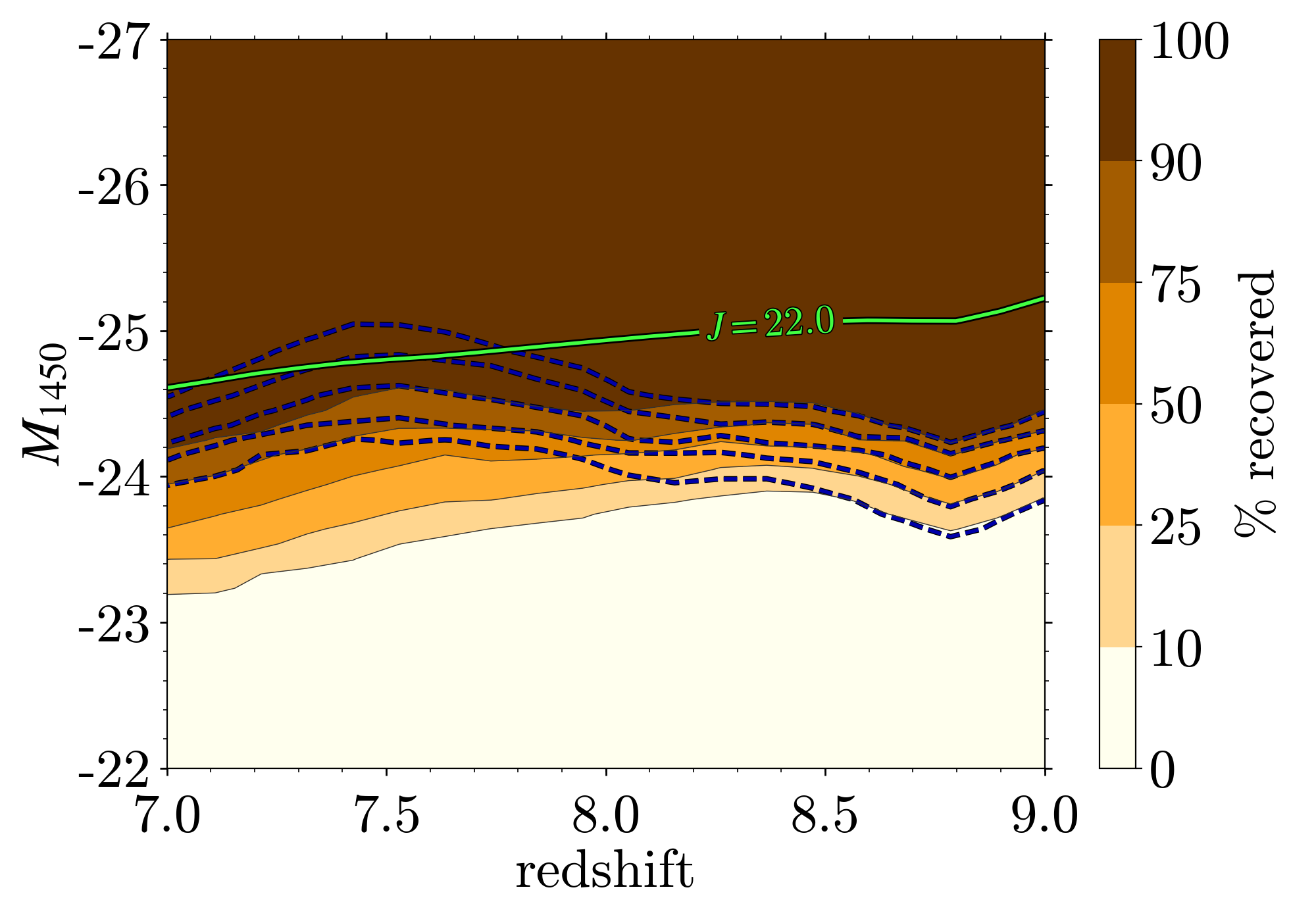
Figure 10: Quasar selection functions determined using BMC (filled contours; same as Fig. 8b) and $\chi^{2}$ model fitting (dashes), assuming $z$-band data are available. Contour intervals are the same in both cases.

Following the procedure described in Sect. 3.1.2, we additionally measure quasar selection using minimum-$\chi^{2}$ model fitting. We integrate QLFs over these new selection functions, and present the resulting numbers in redshift bins in Table 3. Taken as a whole, the BMC method significantly outperforms the $\chi^{2}$ model fitting. In general, the inclusion of surface density information for each population improves the depth to which one is able to select high-redshift quasars (Mortlock et al., 2012).

However, as seen in the selection functions in Fig. 10, the differences in the contours depend on redshift. At lower redshifts $7<z<8$ the BMC contours in Fig. 10 are around $0.5$ mag. deeper than the contours of the $\chi^{2}$ method, and the yield is around a factor of two greater (Table 3). By contrast, at $z\gtrsim 8.2$ the methods apparently perform equally well, as quasars are easily separated from other populations on the basis of $Y-J$, meaning contaminant models are always poor fits to the simulated photometry. As such, the predicted quasar yield is very similar for both methods between $z={8.0}\,\textrm{--}\,{8.5}$, and at $z>8.5$ the predicted numbers are the same using either method. In Sect. 4.3 we explore relaxing the selection cuts of the $\chi^{2}$ method to produce a deeper sample. However, doing so (while keeping contamination low) does not significantly improve quasar selection over $7.0<z<8.0$, meaning the predicted number counts remain lower than for the BMC method. We conclude that the absence of prior population information in the $\chi^{2}$ method places a limit of $J\sim 22.5$ on the quasars $7.0<z<8.0$ that can be detected in Euclid in this way.

4.3 Sample contamination

An important further consideration is the selection of contaminants in the Euclid wide survey, i.e., the number of MLTs and early-type galaxies that pass our selection criteria. We simulate a realistic number of contaminants over the full wide survey area, with magnitudes (both populations) and redshifts (ellipticals only) drawn from the surface density functions described in Sect. 3.2. The sources that we generate have a true $J$ magnitude up to one magnitude fainter than the survey limit, to allow sources to scatter bright when we simulate the noisy photometry. In total, we simulate $8.6\times 10^{7}$ MLTs, and $4.8\times 10^{7}$ ellipticals with $1<z<2$. To make the $P_{\mathrm{q}}$ calculation more manageable, and to focus on the sources that are most likely to be of interest, we take a cut on $\chi^{2}$, discarding all sources that are reasonably well fit by any contaminant template SED ($\chi^{2}_{{\rm red,c(best)}}<5$). The remaining sample contains $6.1\times 10^{5}$ MLTs, and $1.5\times 10^{5}$ galaxies. We apply the BMC method to these samples, assuming that ground-based data are available. In total, we recover 147 sources with $P_{\mathrm{q}}>0.1$. The majority (126) are brown dwarfs, with 21 galaxies additionally recovered. The dwarf stars have spectral types between M9 – T7, although more than 75% of these sources are in the range T2 – T4. Later T-types are much bluer than quasars in $J-H$, which is typically sufficient to discriminate between the two populations. The $z-Y$ colour of the recovered sources has typically scattered very red, such that $z-Y>3$, making the measured SED of each object a close match to the quasar templates (Fig. 1).

We show the cumulative contaminant numbers using the BMC method as a function of $J$ magnitude as the black dotted line in Fig. 9b. This prediction should be compared to the red curves, which are also based on the availability of ground-based $z$-band data. Brighter than $J=22.5$ the number of recovered contaminants is very low, suggesting quasars will be very efficiently recovered at these magnitudes. However, as the S/N falls further, the contamination starts to increase. Using BMC, the majority of quasars detected by Euclid will be brighter than $J=23$. At this magnitude limit, the implied selection efficiency, defined as the ratio of quasars to the total number of selected sources, will be around two thirds, depending on the exact QLF evolution. By $J=24$, the number of contaminants is comparable to the predicted quasar numbers for $k=-0.92$, implying a selection efficiency of around a half.

In the case where only Euclid optical data are available, the number of contaminants is seen to fall, e.g., we now select 50 brown dwarfs with spectral types M9 – T7 with $P_{\mathrm{q}}>0.1$. The numbers are similar to the case where the $z-Y$ colour is used as faint as $J\sim 22.7$; however, few sources are selected fainter than this limit when using the $O$ band in the BMC calculation rather than $z$. This is a similar picture to the quasar numbers as a function of magnitude presented in Fig. 9b. As discussed in Sect. 2.2, the $z-Y$ colour straddles the the Ly$\alpha$ break more closely than $O-Y$, improving the contrast between populations, and so enhancing our sensitivity to quasars. This allows the search for quasars to go deeper, at the expense of additional contamination.

Repeating the analysis (with $z$-band data) for the $\chi^{2}$ method, the total number of contaminants is 25 using the cuts in Sect. 3.1.2, implying a high selection efficiency at all magnitudes (although the BMC method is comparably efficient brighter than $J=22.5$, the limit of the $\chi^{2}$ method discussed in Sect. 4.2). This might suggest that the $\chi^{2}$ cuts could also be relaxed, to allow a deeper search for quasars in Euclid, but a preliminary analysis indicates this is not fruitful. As a test we re-calculated the predicted numbers of quasars and contaminants with slightly looser cuts: $\chi^{2}_{{\rm red,c(best)}}>9$; and $\chi^{2}_{{\rm red,c(best)}}/\chi^{2}_{{\rm red,q(best)}}>2.5$. Doing so increased the contamination by factor of three, while the number of quasars increased only by around $10\%$, driven by a very small improvement over $7<z<8$. In summary the $\chi^{2}$ method has similar effectiveness to the BMC method over the magnitude and redshift range over which it is sensitive, Fig. 10, but the BMC method results in much higher predicted numbers of quasars because it reaches 0.5 mag. deeper over the redshift range $7<z<8$.

The observed decline in selection efficiency with apparent magnitude will have a bearing on future follow-up strategy, which we discuss further in Sect. 5.3. However, follow-up will prioritise the highest probability candidates, which will typically be the brightest. If future follow-up resources are limited then, e.g., a magnitude cut can be applied to ensure a complete sample and allow measurements of the QLF.

5 Discussion

The quasar yield predicted in Sect. 4 and summarised in Table 3 confirms that Euclid can make a major contribution to EoR science in the 2020s. We now explore some of the implications of the simulation work presented in this paper. In Sect. 5.1 we discuss the likely timeline for quasar discoveries with Euclid. In Sect. 5.2 we consider the extent to which Euclid can constrain the QLF. In Sect. 5.3 we explore some of the challenges in terms of the follow-up of Euclid high-redshift quasar candidates.

We additionally examine some of the uncertainties that have a bearing on the calculation presented in this work. In Sect. 5.4 we use COSMOS data to further investigate our choice of contaminating populations in this work. In Sect. 5.5 we consider to what extent the assumptions made about the early-type galaxy population influence the predicted numbers. In Sect. 5.6 we explore the extent to which quasar selection using Euclid is affected by the range in quasar properties. We find that neither of these uncertainties is important, and the dominant uncertainty in the calculations presented here is the value of the parameter $k$.

5.1 Potential status mid-2020’s

Table 4: Potential quasar yield in redshift bins, following the Euclid DR1 release planned for 2024. Numbers are determined over $1250\,{\rm deg}^{2}$ of the southern hemisphere, assuming LSST one-year data are available in the optical. Results are shown for two evolutions of the QLF.

Redshift range	$k=-0.72$	$k=-0.92$
$7.0<z<7.5$	18.8	10.7
$7.5<z<8.0$	4.1	1.8
$8.0<z<8.5$	1.5	0.5
$8.5<z<9.0$	0.6	0.2
Total	24.9	13.2

With the launch of Euclid currently planned for mid 2022, and the full $15\,000\,{\rm deg}^{2}$ of wide survey not expected to be available until some seven years after launch (3 data release; DR3), it will be over a decade before the number count predictions in this paper are fully realised. Nevertheless, intervening data releases will offer opportunities to carry out excellent quasar science. Importantly, the desired wide survey depth for each tile is achieved in a single visit, while the area is built up over time; hence the selection functions are applicable to all Euclid releases, depending on the availability of complementary optical data. The first Euclid quick release (Q1) is expected around 14 months after the start of survey operations, and will only cover a small area, with the exact size and location yet to be determined. However, assuming $k=-0.72$, and an area of $50\,{\rm deg}^{2}$, the predicted yield, $7<z<9$, is at most one quasar, even when $z$-band data are used. Nevertheless, Q1 data will offer an opportunity to test the proposed selection methods, and get a sense of the expected contamination rate when applied to real data.

This assessment of the predicted quasar numbers from Q1 has assumed that data from this initial release will match the wide survey depth, i.e., $YJH=24$. We have not considered the possibility that these fields form part of the Euclid deep survey, which will ultimately go two magnitudes fainter than the wide survey in all bands However, as mentioned in Sect. 2.1, deeper observations would not make a significant difference to the predicted numbers for Q1. In principle, the quasar yield would be maximised by surveying a wider area, rather than going deeper. The single visit depth of $J=24$ means for $z={7}\,\textrm{--}\,{9}$ quasars, we are already sampling the faint-end slope of the QLF ($M_{1450}>-24.9$, Matsuoka et al., 2018c). Without any consideration of completeness, the Jiang et al. (2016) QLF integrated to $J=24$ implies one $z={7}\,\textrm{--}\,{9}$ quasar per $20\,{\rm deg}^{2}$. Going one magnitude fainter, this density increases to one $z={7}\,\textrm{--}\,{9}$ quasar per $8\,{\rm deg}^{2}$, but the additional depth would require six observations of the field to achieve.

Looking further ahead, Euclid DR1, comprising the first year of survey data, is anticipated in the second year after the nominal mission start (i.e., mid-2024). DR1 should cover $2500\,{\rm deg}^{2}$ in total, split equally between the northern- and southernmost sky. In the northern hemisphere, Pan-STARRS is only expected to have reached a $5\sigma$ depth of $z=24.1$ by DR1; hence, selection will be somewhat worse over $z={7}\,\textrm{--}\,{8}$ than assumed in Fig. 8b. However, access to one-year LSST data is a realistic prospect. In Table 4 we present predicted numbers for the southern hemisphere following DR1, assuming LSST data are available, and assuming that an area of $1250\,{\rm deg}^{2}$ is covered by LSST. Even with stronger redshift evolution, $k=-0.92$, the quasar yield from DR1 will potentially be significant, especially when combined with additional discoveries from the northern hemisphere. We would anticipate considerably more than ten sources over the redshift range $7<z<9$, which would potentially include the first discoveries at $z>8$, from the full DR1 area. DR1 will therefore likely be an exciting prospect for high-redshift quasar science, with scope for significant development with subsequent Euclid data releases.

5.2 Quasar luminosity function constraints

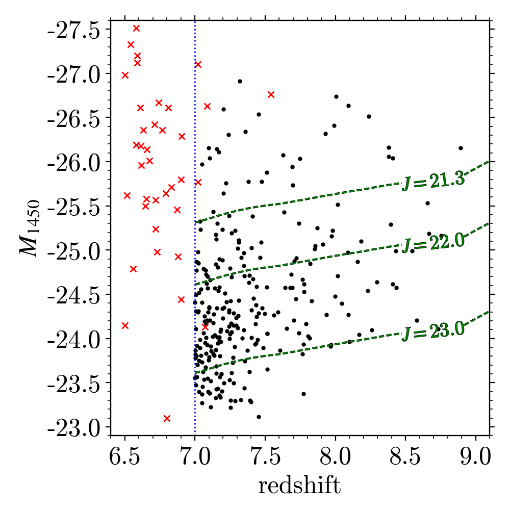
Figure 11: $M_{1450}\,/\,z$ plane with all $z>6.5$ quasars with published redshifts and luminosities at 1450 Å (red crosses), and a simulated Euclid wide survey quasar sample (black points), with random luminosities and redshifts drawn from the ground-based selection function (Fig. 8b). The blue dotted line indicates the redshift cut-off of this work. The green dashed contours indicate the apparent magnitudes considered in Sect. 5.3, in the context of ground-based follow-up spectroscopy and contamination. Discovery papers for the known quasars are: Mortlock et al. (2011); Venemans et al. (2013, 2015); Matsuoka et al. (2016, 2018a, 2018b, 2019); Mazzucchelli et al. (2017); Tang et al. (2017); Koptelova et al. (2017); Reed et al. (2017); Wang et al. (2017, 2018a, 2018b); Bañados et al. (2018); Yang et al. (2019).

A sample of Euclid $z>7$ quasars will provide constraints on the QLF. To illustrate the potential of Euclid, we simulate a full wide survey quasar sample, assuming $k=-0.72$ and that $z$-band data are available, with redshifts and magnitudes drawn from the distributions in Fig. 9. We plot the redshifts and luminosities of this simulated sample in Fig. 11, shown alongside all $z>6.5$ quasars which have been published to date (references in caption).

Fig. 11 illustrates the redshifts and luminosities at which Euclid will have a particularly large impact. The Euclid wide survey will be especially useful for measuring the redshift evolution of the quasar number density, parametrised by $k$. Previous works have used bright ($M_{1450}<-26$) quasars to determine $k$ (e.g. Fan et al., 2001a; McGreer et al., 2013; Jiang et al., 2016); however, by the time Euclid data are available, the $6.5<z<7$ QLF is likely to be sufficiently well determined to measure the evolution of number density at fainter magnitudes (see, e.g., Matsuoka et al., 2018c). As an illustrative example, we consider the constraints that can be put on $k$, assuming the number density has been well measured to a depth of $M_{1450}=-25$ over $6.5<z<7.0$. The simulated Euclid sample contains 24 $7.5<z<8.5$ sources with $M_{1450}<-25$. Assuming $k=-0.72$ represents the true redshift evolution over $z={7}\,\textrm{--}\,{8}$, the Euclid sample implies we could measure $k$ to a $1\sigma$ uncertainty of 0.07 over that redshift range.

Euclid will also place strong constraints on the faint end of the quasar luminosity function. At $z=6$, the characteristic ‘knee’ magnitude, $M^{*}_{1450}$, was recently well constrained by Matsuoka et al. (2018c, $M^{*}_{1450}=-24.9^{+0.75}_{-0.90}$ mag); the same authors also obtained a faint-end slope, $\alpha=-1.23^{+0.44}_{-0.34}$. As illustrated in Fig. 11, Euclid will produce a large sample of quasars $7<z<8$ fainter than $M_{1450}=-25$, which will allow the faint-end slope to be measured precisely over this redshift range, and also allow the evolution of the break from $z\sim 6$ to $z>7$ to be determined.

5.3 Follow-up demands

Confirmation and exploitation of the high-redshift quasar candidates identified by Euclid will require follow-up spectra, e.g., to measure the redshifts, and to study the Ly$\alpha$ damping wing to measure the cosmic density of neutral hydrogen. We use the Euclid selection function to determine predicted numbers as a function of $J$, as in Fig. 9b, but for the separate ranges $z={7}\,\textrm{--}\,{8}$, and $z={8}\,\textrm{--}\,{9}$. In both redshift bins, the median magnitude is $J\sim 22.5$, while the 10 and 90 percentiles are respectively $J\sim 21.3$ and $J\sim 23.3$, which we take to be indicative of the typical range of depths that we would need to reach. For a particular high-redshift quasar, two spectra might be required: the first to confirm the candidate, and a second, higher S/N spectrum, to measure the damping wing. As a fiducial value, we adopt the requirement that confirmation that a source is a quasar, even if weak lined, and measurement of a redshift, requires an observed S/N $\gtrsim 1.2$ per Å, in the continuum, over a wide wavelength range. A spectrum for measuring the damping wing would require S/N $\gtrsim 4$ per Å, or an integration time ten times longer than required for identification.

Using these numbers and allowing for a maximum of 3 h integration time to classify any candidate, a campaign of spectroscopic confirmation of Euclid sources down to $J=22$ with 8 m class telescopes would be feasible. Some sources with strong lines that are fainter than $J=22$ could be identified, but we are mainly interested in creating a complete sample, in order to measure the luminosity function. This calculation is somewhat conservative. It is based on data taken with the Gemini GNIRS instrument, assuming mediocre seeing conditions (up to $1$\mathrm{\SIUnitSymbolArcsecond}$$), as might be appropriate as a specification for a large programme. It would be possible to reach deeper in better seeing (see, e.g., the results achieved by Kriek et al. 2015). Allowing for 10 h observing time per source to measure the damping wing, a campaign of spectroscopy to measure the cosmic neutral fraction as a function of redshift, and its variance, could reach $J=21.3$ with 8 m class telescopes. These two limits are marked by lines in Fig. 11.

This analysis illustrates the difficulty of completing all the potential high-redshift quasar science with 8m class telescopes. To confirm sources fainter than $J\sim 22$, and to measure the faint end of the quasar luminosity function will require future facilities such as the James Webb Space Telescope (JWST) or the European Extremely Large Telescope. At very faint magnitudes ($J\sim 23$), where the number of contaminants may be comparable to the number of quasars (Sect. 4.3), it seems likely that a spectroscopic campaign would need to be limited to a subset of the candidates. The limits presented in this discussion are illustrative only, and the approach to follow-up will naturally depend on the details of future candidate lists, and the availability of follow-up resources.

It will be possible to identify some of the brightest candidates using the slitless spectra obtained with the Euclid NISP instrument, but the wavelength coverage of the instrument is no longer very well suited to this task. NISP will produce slitless (R = 380) spectra of all sources in the wide survey. The NISP red grism originally covered the wavelength range (${1.1}\,\textrm{--}\,{2.0}\,$\mathrm{\SIUnitSymbolMicro m}$$) (Laureijs et al., 2011), and for this configuration Roche et al. (2012) showed how high-redshift quasars $z>8$ could be identified by the continuum break at Ly$\alpha$. In the new configuration the wavelength coverage is (${1.25}\,\textrm{--}\,{1.85}\,$\mathrm{\SIUnitSymbolMicro m}$$), and the Ly$\alpha$ break is outside this range for all redshifts of interest $7<z<9$. Quasars in this redshift range might still be identified by the detection of C iv 1549 and $\left.{\rm C}\,\textsc{iii}\right]$ 1909. To explore this approach further, we ran exploratory simulations using an early version of the Euclid simulator of the NISP, named TIPS (TIPS Is a Pixel Simulator; Zoubian et al., 2014). These simulations consisted in producing 2D grism images of the observed spectrum of ULAS J1120+0641 (Mortlock et al., 2011, $J=20.2$), and did not include source contamination. Simple image stacks and visual inspection suggested that sources with $J<21$ could be identified by this means.

5.4 Choice of contaminating populations

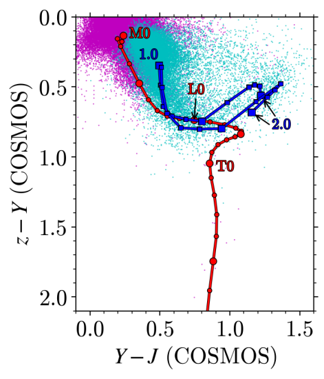
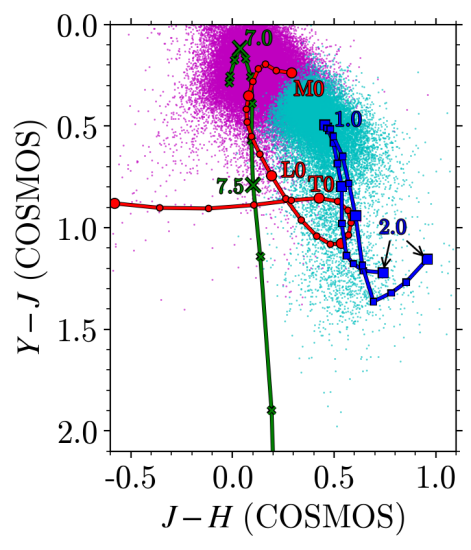
Figure 12: Model COSMOS colour tracks and COSMOS sources. The COSMOS filters are different to Euclid and LSST/Pan-STARRS, resulting in slight differences in the tracks presented in Fig. 1. The individual population models are however indicated in the same way as in that figure: the red tracks show MLTs; the early-type elliptical tracks are blue; and the quasar track is green. We additionally plot sources brighter than $J=23$ in the COSMOS catalogue (Laigle et al., 2016). Magenta points indicate sources with photometry best fit by an MLT model. The cyan points indicate sources with photometry best fit by an elliptical galaxy model. Upper: $zYJ$ colours. Lower: $YJH$ colours.

The predictions in this work are based on the assumption that the relevant population space for high-redshift quasar searches can be reduced to the target quasars, and two types of contaminants: namely, MLTs and elliptical galaxies. These populations have long been known as important sources of contamination for $z>7$ quasar searches (e.g. Hewett et al., 2006). MLTs and ellipticals are expected to be abundant in Euclid, and as seen in Fig. 1, their near-infrared colours match closely to those of quasars. One might ask, however, whether this fully represents the range of populations present in real data that might have a bearing on quasar selection.

To investigate this question we return to the COSMOS sample presented by Laigle et al. (2016), which we used in Sect. 3.2.3 to model the elliptical surface density. We determine model $zYJH$ COSMOS colours from our population templates, and show these tracks in Fig. 12, along with the 77 000 sources brighter than $J=23$ in the COSMOS catalogue. Fig. 12 indicates that our choice of contaminant templates encapsulates the red envelope of the COSMOS sources very well. We do not see evidence for a significant additional population that is very red in $z-Y$ (where the reddest sources follow the T-dwarf track closely), or in $Y-J$, although in the latter case, a few sources appear to scatter towards $Y-J\sim 2$, consistent with $z>7.7$ quasars.

As a further check we apply our minimum-$\chi^{2}$ selection method to the COSMOS sources. Despite the depth of the COSMOS survey, the small area ($<1.5\,{\rm deg}^{2}$) means we do not expect any $z>7$ quasars to be present in the catalogue. Therefore any significant number of candidates that are better fit by a quasar template would likely be indicative of an additional population that needs to be accounted for in our selection methods. However, on the basis of our SED fitting, all sources are classified as either an MLT or as an elliptical galaxy, respectively indicated in magenta and cyan in Fig. 12. This result lends support to the above statement that there is no significant additional contaminating population in the COSMOS data. We note our ability to distinguish quasars from contaminants is in this case helped by very deep COSMOS $z$-band data. Nevertheless, in general terms these preliminary results indicate that our models are representative of the populations that will be of concern once Euclid data are available.

5.5 Importance of the early-type galaxy population

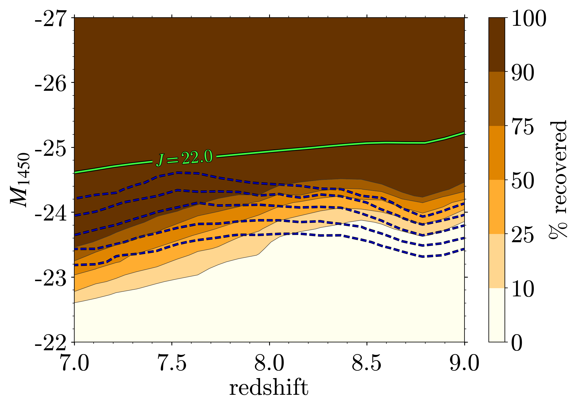
Figure 13: Quasar selection functions using ground-based data and using BMC, assuming a single contaminating population. Filled contours indicate the case where only galaxies are considered as contaminants, i.e., $W_{\mathrm{s}}=0$. Dashed lines indicate the case where only MLTs are considered, i.e., $W_{\mathrm{g}}=0,W_{\mathrm{s}}\neq 0$. Contour intervals are the same in both cases. The contour indicating $J=22$ is also shown as a solid green line.

In Sect. 3.2.3 close attention was paid to the sizes of early-type galaxies in the redshift range of interest $1<z<2$. We were motivated by the concern that faint ($J>22$) galaxies may be mistaken for point sources, given the relatively large pixel size of the Euclid NISP instrument, and the small half-light radii of the galaxies at faint magnitudes. Based on the predicted sizes we conservatively assumed that all faint $J>22$ early-type galaxies would be classified as point sources. We now consider whether this assumption is significant in terms of the predicted quasar numbers.

To proceed, we produce two further selection functions, for the case where ground-based $z$-band data are available, i.e., to be compared with Fig. 8b. In each case we switch off the effect of either the MLT or elliptical population. That is to say, we set either $W_{\mathrm{s}}$ or $W_{\mathrm{g}}$ equal to zero when calculating $P_{\mathrm{q}}$. We present the resulting two selection functions in Fig. 13. In this plot the MLT selection function (i.e., where MLTs are the only contaminating population) is shown by the dashed lines and the ellipticals selection function as the solid lines. At any redshift the population that dominates the contamination, and controls the quasar detection probability, is the population where the contours are higher up the plot (towards brighter magnitudes). Since the assumptions we have made about the early-type galaxies have been conservative, the true contours for this population are somewhat lower down the plot.

At $z<8$, the MLT population dominates the selection function, i.e., the assumptions about the early-type galaxies have no influence on the predicted quasar numbers over the MLTs. At higher redshifts, the situation changes. At $z\sim 8$ the contours cross, meaning the two populations contribute approximately equally, while at $z>8.2$ the overall selection function is constrained more tightly by the ellipticals, but not by much. This indicates that even if it is possible to eliminate most of the early-type galaxies within the Euclid pipeline on the basis of morphology, the improvement in the number of quasars detectable will be fairly modest. To test this, we integrated the QLF over the dashed selection function in Fig. 13 (with $W_{\mathrm{g}}=0$), to evaluate the predicted quasar numbers with MLTs as the sole contaminant. Compared to Table 3, we find a negligible change for $z<8$, while the predicted counts at $z>8$ increase by $25\%$.

5.6 Variations within the quasar population

Table 5: Weights for each value of line width and continuum slope, used to combine the individual Euclid quasar selection functions. The total weight of a single quasar model is given by the product of the relevant slope and line width.

parameter	model value	weight
line width	half	0.3
	standard	0.6
	double	0.1
continuum slope	blue	0.05
	standard	0.7
	red	0.25

In simulations of the quasar selection function so far we have made a simplifying assumption by only using a single typical model spectrum to generate synthetic quasar colours. We have not considered variations in the continuum and line emission. As explained in Sect. 3.2.1, the reason for using a single model quasar is for simplicity, because this still yields accurate estimates of the quasar yield (e.g., Barnett et al. in prep.). In this subsection we explore the sensitivity of the selection function calculation to a mismatch between the actual quasar colours, and the model used in the selection. To proceed, we model quasars with a range of spectral types, and consider selection using a single, typical type. In the actual search we will use an appropriate range of model spectra in the selection, so the calculation presented here will overestimate the effect of spectral mismatch. Nevertheless it gives a sense of the scale of the problem of a mismatch between the actual quasar SEDs and those assumed in the selection algorithm, and so gives an indication of the proportion of quasars that might be missed if the spectra of quasars at $z>7$ are more diverse than at lower redshifts.

The Hewett et al. (2006) and Maddox et al. (2008) quasar models are available for a range of continuum slopes and emission line strengths. We now wish to produce selection functions for quasar populations with different properties, and compare the resulting numbers with those presented in Sect. 4. Explicitly, the typical quasar spectrum that we have used so far has a line strength with rest frame $\mathrm{EW_{{\rm C}\,\textsc{iv}}=39.1\,\AA}$ and UV continuum slope $f_{1315}/f_{2225}=cs=1.0$. We now additionally make use of models with doubled and halved line strengths, and blue and red continuum slopes corresponding to $cs=1.16$, and 0.84 respectively. Broad absorption line quasars are effectively included here, as the colours would be matched by weak-lined objects with red continua. We therefore have nine combinations of line widths and slopes in total. Following the previous prescription we simulate grids of quasars for each type, using the Euclid $O$ band in the optical. We then determine selection functions and combine them, with the weight for each value of line width and continuum slope given in Table 5. These weights are based on the distribution of slopes and line widths measured for SDSS DR7 quasars, i.e., representative of the quasar population at redshifts $0<z<6$. Conceivably the distributions of line widths and continuum slopes in the quasar population at $z>7$ may prove to be somewhat different (see, e.g., the evidence for a larger fraction of sources with weak C iv emission at $z>6$ presented by Shen et al. 2019), in which case the relative weights in the selection, or indeed the models themselves, can be adjusted.

Integrating the Jiang et al. (2016) QLF ($k=-0.72$) over the resulting selection function, there is a clear impact on the predicted numbers when there is a mismatch between the quasar template(s) used in the selection method, and the actual quasar SEDs. The total yield over $7<z<9$ is reduced by $20\%$, compared to the total of 124 sources predicted previously (Table 3, column 1). This decrease is driven by slightly worse selection at $z<8$.

In contrast, preliminary simulations suggest that incorporating the full range of quasar templates in the BMC method mitigates substantially against this reduction in numbers, as stated previously. In this case, we draw 1000 quasars distributed uniformly in redshift and luminosity space from each of the nine grids described above. We then determine $P_{\mathrm{q}}$ values for these quasars using all nine SEDs in the BMC, weighting the contribution of each SED to $W_{\mathrm{q}}$ using the values in Table 5. We find the number of recovered quasars is almost identical to the case where we use just the typical model both to generate synthetic quasars and in the BMC (i.e., as in the rest of the paper). The results from this section therefore highlight the need for a realistic range of model templates in our selection methods, in order to maximise the future quasar yield with Euclid.

6 Summary

In this paper we have presented a detailed study of the use of the $15\,000\,{\rm deg}^{2}$ Euclid wide survey for the discovery of quasars in the redshift range $7<z<9$, updating the predicted quasar yield presented by Laureijs et al. (2011). This work incorporates revisions to the NISP filter wavelengths and the planned survey area, and accounts for the steeper redshift evolution of the quasar number density, based on the decline measured over $z={5}\,\textrm{--}\,{6}$ by Jiang et al. (2016). We have extended the Laureijs et al. (2011) analysis, that considered redshifts $8<z<9$, to include the range $7<z<8$, and we have improved the earlier study in two important ways: candidate quasars are now selected using statistical methods rather than heuristic colour cuts, allowing the detection of fainter high-redshift quasars; and we have developed more accurate models of the contaminant populations, i.e., MLT dwarfs, and early-type galaxies at redshifts $1<z<2$.

The main results of this paper are based on simulations of Euclid quasar selection functions and contaminating populations, and are summarised below.

1. Quasars with redshifts $8<z<9$ can be selected from Euclid data alone. Even if the rate of decline in the space density of quasars accelerates beyond $z=6$, and is as steep as $\Phi\propto 10^{k(z-6)}$, $k=-0.92$, there should be some 6 quasars discoverable with Euclid at $z>8$, brighter than $J\sim 23$, using Euclid data alone, improving to 8 quasars if deep ground based data is available.

2. Deep ground-based $z$-band data from LSST and Pan-STARRS significantly boost the selection of quasars over $7<z<8$, compared to using the Euclid $O$ optical band, due to the sharper contrast for a spectral break to the blue of the $Y$ filter. Using the expected depths for the optical surveys, we find that Euclid will discover more than 100 quasars $7<z<8$, assuming $k=-0.92$. If $z$-band data are not available, the total return is smaller by a factor greater than two.

3. Both the BMC and minimum-$\chi^{2}$ method are able to eliminate the majority of contaminants, although at lower S/N contamination from MLTs and ellipticals needs to be considered and may impact future follow-up strategy. Over the redshift range $7<z<8$, the inclusion of priors means the BMC method can reach at least 0.5 mag fainter than the simpler minimum-$\chi^{2}$ method, resulting in a factor of two difference in the total predicted numbers.

4. The rate of decline of the QLF, parametrised by $k$, is the most significant unknown for the number count predictions. If $k=-0.72$ over the redshift range $7<z<8$ this parameter will be measured to a $1\sigma$ uncertainty of 0.07.

We anticipate that, except for the brightest sources, spectroscopic follow-up of Euclid quasar candidates will generally be challenging with existing ground-based 8 m telescopes. Nevertheless, beginning with Euclid Data Release 1, planned for 2024, we expect significant numbers of $z>7$ quasars to be discovered with Euclid, allowing detailed studies of the cosmic neutral fraction of hydrogen over redshifts $7<z<9$, which will make an important contribution towards understanding the process of cosmic reionisation. These new samples will also be valuable for studies of early SMBH growth, from the measurement of black hole masses in individual sources and through additional constraints on the faint end of the QLF. Conceivably for some sources it may prove possible to image the IGM structure surrounding the quasar in the light of Ly$\alpha$.