The Hubbard model on the honeycomb lattice: from static and dynamical mean-field theories to lattice quantum Monte Carlo simulations

Abstract

We study the one-band Hubbard model on the honeycomb lattice using a combination of quantum Monte Carlo (QMC) simulations and static as well as dynamical mean-field theory (DMFT). This model is known to show a quantum phase transition between a Dirac semi-metal and the antiferromagnetic insulator. The aim of this article is to provide a detailed comparison between these approaches by computing static properties, notably ground-state energy, single-particle gap, double occupancy, and staggered magnetization, as well as dynamical quantities such as the single-particle spectral function. At the static mean-field level local moments cannot be generated without breaking the SU(2) spin symmetry. The DMFT approximation accounts for temporal fluctuations, thus captures both the evolution of the double occupancy and the resulting local moment formation in the paramagnetic phase. As a consequence, the DMFT approximation is found to be very accurate in the Dirac semi-metallic phase where local moment formation is present and the spin correlation length small. However, in the vicinity of the fermion quantum critical point the spin correlation length diverges and the spontaneous SU(2) symmetry breaking leads to low-lying Goldstone modes in the magnetically ordered phase. The impact of these spin fluctuations on the single-particle spectral function – waterfall features and narrow spin-polaron bands – is only visible in the lattice QMC approach.

I Introduction

The one-band “Hubbard” model Hubbard (1963); Kanamori (1963); Gutzwiller (1963); Tasaki (1998); Eder (2017) is one of the basic models for correlation effects in solids. Its square-lattice version has been investigated extensively because of its relevance to the high-temperature superconductors Dagotto (1994); Brenig (1995). Screened electronic correlations modeled by a Hubbard-$U$ term generate local magnetic moments. For the half-filled band, local moments generically order and the global SU(2) spin symmetry is spontaneously broken leading to Goldstone modes. The interplay of charge and spin degrees of freedom is the key point captured by the Hubbard and strong-coupling $t$-$J$ models. For the well-studied single-hole problem, the single-particle spectral function of the square-lattice Hubbard and $t$-$J$ models reveals spin polaron quasiparticles as well as “waterfall” features Preuss et al. (1995, 1997); Brunner et al. (2000). These anomalous spectral properties and their evolution with doping have been the subject of extensive numerical studies Kyung et al. (2006); Macridin et al. (2007); Zemljič et al. (2008); Wróbel et al. (2008); Moritz et al. (2010); Sakai et al. (2010); Dalla Piazza et al. (2012); Rost et al. (2012); Kohno (2014); Yang and Feiguin (2016); Wang et al. (2018).

For the half-filled Hubbard model on the square lattice, perfect nesting drives the system into an antiferromagnetic phase for any finite on-site repulsion $U>0$ Hirsch (1985); White et al. (1989). By contrast, while the honeycomb lattice is also bipartite, the half-filled Hubbard model on this lattice is distinguished by a vanishing density of states at the Fermi level such that a finite $U$ is required to drive the system into the antiferromagnetic phase that is expected for large $U$, as was already remarked in the seminal work Ref. Sorella and Tosatti (1992). On the one hand, having access to a transition from a Dirac semi-metal to an antiferromagnet at a finite value of $U$ is interesting from a fundamental point of view since it allows one, e.g., to study the critical properties. On the other hand, graphene Geim and Novoselov (2007); Castro Neto et al. (2009); Yazyev (2010); Wakabayashi (2013) is believed to be well described by the Hubbard model on the honeycomb lattice in its semi-metallic phase such that weak-coupling methods remain appropriate tools.

Extensive numerical studies of the phase diagram of the half-filled Hubbard model on the honeycomb lattice Sorella and Tosatti (1992); Meng et al. (2010); Sorella et al. (2012); He and Lu (2012); Hassan and Sénéchal (2013); Seki and Ohta (2013); Assaad and Herbut (2013); Wu and Tremblay (2014) have led to the consensus that the transition between the paramagnetic semi-metal and the antiferromagnetic insulator is a direct one with an unusual quantum critical point separating these two phases. The critical behavior is captured by a Gross-Neveu-Yukawa field theory Herbut et al. (2009), consisting of eight-component Dirac fermions Ryu et al. (2009) as well as a three-component $\phi^{4}$-theory accounting for the magnetic order parameter and low-lying long-wave-length Goldstone modes. The Yukawa term couples the three-component bosonic modes to the triplet of antiferromagnetic mass terms such that when the bosons condense fermion mass is generated. The upper critical dimension for this theory is of three spatial dimensions such that an $\epsilon$-expansion can be used to calculate the deviation of the critical exponents from the mean-field results in two dimensions Herbut et al. (2009).

The aim of this paper is to provide a detailed comparison between various approximations and numerically exact quantum Monte Carlo (QMC) results for the Hubbard model on the honeycomb lattice. We will start with the mean-field approximation that is widely used in the context of graphene, see Refs. Yazyev (2010); Wakabayashi (2013); Feldner et al. (2010); *FeldnerE and references therein. The first clear shortcoming of this approximation is the failure to generate local moments without breaking the SU(2) spin symmetry. The minimal extension of the static mean-field approximation to account for local moment formation is dynamical mean-field theory (DMFT). Provided that the magnetic correlation length is not too big, DMFT is expected to provide a good account of the physics, and thus promises improved numerical accuracy in the parameter regime relevant to graphene at a moderate computational cost.

Early single-site DMFT studies located the metal-insulator transition around $U_{c}/t\gtrsim 10$ Jafari (2009); Tran and Kuroki (2009). This is not only significantly above the mean-field transition $U_{c}/t\approx 2.23$ and the early QMC estimate $U_{c}/t=4.5\pm 0.5$ Sorella and Tosatti (1992), but also much larger than the most accurate QMC results, namely $U_{c}/t\approx 3.87$ Sorella et al. (2012) and $U_{c}/t\approx 3.78$ Assaad and Herbut (2013), respectively. Consequently, further investigations of the semi-metal–antiferromagnet transition in the Hubbard model on the honeycomb lattice focused on cluster and other extensions of DMFT He and Lu (2012); Hassan and Sénéchal (2013); Seki and Ohta (2013); Liebsch and Wu (2013); Wu and Tremblay (2014); Hirschmeier et al. (2018), and the corresponding estimates for the location of the transition converge to the region $U_{c}/t\approx 3.6\ldots 3.8$ Wu and Tremblay (2014); Hirschmeier et al. (2018), see Ref. Hirschmeier et al. (2018) for a more detailed summary. These estimates from different generalizations of DMFT are indeed very close to the QMC estimates. However, the single-site studies Jafari (2009); Tran and Kuroki (2009) only looked at paramagnetic solutions. Thus, to the best of our knowledge, the accuracy of the simple single-site DMFT when one allows for the relevant antiferromagnetic solution at large $U$ has not been investigated in the literature. Hence, we implement this here and benchmark it against QMC results on the lattice.

Furthermore, the spectral functions of the Hubbard model on an infinite honeycomb lattice are in principle well known, at least at the mean-field level, but to the best of our knowledge they have not been explicitly shown in the literature. Hence, we will discuss mean-field results here, and compare them to more elaborate DMFT and lattice QMC results. Among others, we will show that both the spin-polaron physics and the so-called waterfall features known from the square lattice are also present close to the quantum critical point on the honeycomb lattice, but that QMC simulations are required to reveal them.

The outline of the paper is as follows: In Sec. II we introduce the model and the three methods that we employ for our comparative discussion. Section III focuses on static properties and the dynamical properties are investigated via spectral functions in Sec. IV. We summarize our findings and provide perspectives in Sec. V.

II Model and methods

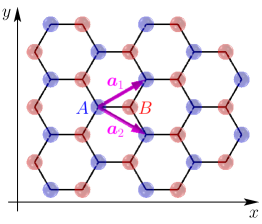
Figure 1: Sketch of the honeycomb lattice showing the two sites $A$ and $B$ in the primitive cell and our choice of primitive vectors $\boldsymbol{a}_{1}$, $\boldsymbol{a}_{2}$.

We study the Hubbard model whose Hamiltonian reads

$$H=-t\sum_{\langle i,j\rangle\atop\sigma=\uparrow,\downarrow}c^{\dagger}_{i,\sigma}c_{j,\sigma}+U\,\sum_{i}\left(n_{i,\uparrow}-\frac{1}{2}\right)\,\left(n_{i,\downarrow}-\frac{1}{2}\right)$$ (1)

with $n_{i,\sigma}=c^{\dagger}_{i,\sigma}c_{i,\sigma}$. Here $\langle i,j\rangle$ are nearest neighbors on a lattice that we take to be the honeycomb lattice illustrated in Fig. 1. We will be interested either in the infinite system, or in a finite but large one. In the latter case, we denote the total number of sites by $N$ and impose periodic boundary conditions.

Note that since the honeycomb lattice is bipartite, the single-band Hubbard model on this lattice is particle-hole symmetric (see, for example, Ref. Scalettar (2016)), i.e., upon exchanging electron creation and annihilation operators, one finds a Hamiltonian that is equivalent to the original one of Eq. (1). This particle-hole symmetry ensures that the global ground state is found at half filling, i.e., for an average of one electron per lattice site.

II.1 Static mean-field theory (MFT)

Many authors have used a real-space Hartree-Fock-type mean-field approximation to study magnetism in graphene, see Refs. Yazyev (2010); Wakabayashi (2013); Feldner et al. (2010); *FeldnerE and references therein. Here, we exploit the SU(2)-symmetry of the original Hubbard model Eq. (1) to align the quantization axis with a possible ordered moment. Then the Hartree-Fock approximation amounts to

$$H^{\rm MF} = -t\sum_{\langle i,j\rangle\atop\sigma=\uparrow,\downarrow}c^{\dagger}_{i,\sigma}c_{j,\sigma}$$ (4)

$$+U\,\sum_{i}\Bigl{(}\langle n_{i,\uparrow}\rangle n_{i,\downarrow}+n_{i,\uparrow}\langle n_{i,\downarrow}\rangle-\langle n_{i,\uparrow}\rangle\langle n_{i,\downarrow}\rangle\quad$$

$$\qquad\quad-\frac{n_{i,\uparrow}+n_{i,\downarrow}}{2}+\frac{1}{4}\Bigr{)}\,.$$

Note that the last term in Eq. (4) could be omitted for most purposes, but it is needed if one wants to compare total energies with the original Hubbard model Eq. (1). The density-dependent term in Eq. (4) ensures half filling in the grand-canonical description thanks to particle-hole symmetry.

Although we have formulated the problem above in real space, here we will actually work in reciprocal space because we are interested in an infinite system. Since the primitive cell contains two sites, we will need to diagonalize a $2\times 2$ matrix for each value of the momentum $\boldsymbol{k}$, followed by a summation over $\boldsymbol{k}$.

To be specific, we first perform a Fourier transformation

$$c_{\boldsymbol{r},\alpha,\sigma}=\sqrt{\frac{2}{N}}\,\sum_{\boldsymbol{k}}{\rm e}^{i\,\boldsymbol{k}\cdot\boldsymbol{r}}c_{\alpha,\sigma}(\boldsymbol{k})\,,$$ (5)

where $\alpha=A,B$ labels the two sites in the primitive cell, $\boldsymbol{r}$ is the real-space position of the primitive cell, and $N/2$ corresponds to the number of primitive cells. We further restrict to half filling and express all the densities in terms of the staggered magnetization $m_{\rm s}$

$$\langle n_{A,\sigma}\rangle=\frac{1}{2}+\sigma\,m_{\rm s}\,,\quad\langle n_{B,\sigma}\rangle=\frac{1}{2}-\sigma\,m_{\rm s}\,,$$ (6)

where we wrote $\sigma=+1$ for the spin up configuration ($\uparrow$) and $\sigma=-1$ for the spin down configuration ($\downarrow$). With these notations and dropping the “constant” term Eq. (4), the mean-field Hamiltonian of Eqs. (4), (4) can now be cast in the form

$$H^{\rm MF}=\sum_{\boldsymbol{k},\sigma}\left(c^{\dagger}_{A,\sigma}(\boldsymbol{k}),c^{\dagger}_{B,\sigma}(\boldsymbol{k})\right)\,\left(\tau_{x}\,\text{Re}z(\boldsymbol{k})+\tau_{y}\,\text{Im}z(\boldsymbol{k})-\ U\,\sigma\,m_{\rm s}\,\tau_{z}\right)\,\begin{pmatrix}c_{A,\sigma}(\boldsymbol{k})\\ c_{B,\sigma}(\boldsymbol{k})\end{pmatrix}\,,$$ (7)

where the Pauli matrices $\tau_{x,y,z}$ act on the “orbital” index $A$, $B$ and $z(\boldsymbol{k})=-t\left(1+{\rm e}^{-i\boldsymbol{k}\cdot\boldsymbol{a}_{1}}+{\rm e}^{-i\boldsymbol{k}\cdot\boldsymbol{a}_{2}}\right)$. Here the primitive vectors are $\boldsymbol{a}_{1}=a\left(\frac{\sqrt{3}}{2},\frac{1}{2}\right)$, $\boldsymbol{a}_{2}=a\left(\frac{\sqrt{3}}{2},-\frac{1}{2}\right)$, compare Fig. 1, and the lattice constant of the underlying triangular lattice is denoted by $a$.

From the $2\times 2$ matrix in Eq. (7) one immediately gets the single-particle dispersion

$$E_{\pm}(\boldsymbol{k})=\pm E(\boldsymbol{k})\text{ with }E(\boldsymbol{k})=\sqrt{\left|z(\boldsymbol{k})\right|^{2}+\left(U\,m_{\rm s}\right)^{2}}\,.$$ (8)

At the Dirac points $\mathbf{K}$ (see inset of Fig. 3(c) below for a definition), we have $z(\mathbf{K})=0$ such that we find the single-particle gap

$$\Delta_{\rm sp}=E(\mathbf{K})=U\,\left|m_{\rm s}\right|\,.$$ (9)

Thus, a finite staggered magnetization leads to the opening of a mass gap in the spectrum.

The staggered magnetization, $m_{\rm s}$, still needs to be determined self-consistently such that Eq. (6) holds. In the following sections, we will use a numerical solution that has been obtained by iteration, i.e., starting with a guess for $m_{\rm s}$, then recomputing it via Eq. (6) until convergence is reached.

On the other hand, we can make analytic progress by considering only low-energy physics. First, we cast the self-consistency condition for $m_{\rm s}$ in the gap equation

$$1=2U\int{\rm d}\epsilon N(\epsilon)\frac{1}{\sqrt{\epsilon^{2}+\Delta_{\rm sp}^{2}}}\tanh\left(\frac{1}{2\,T}\sqrt{\epsilon^{2}+\Delta_{\rm sp}^{2}}\right)$$ (10)

with density of states

$$N(\epsilon)=\frac{2}{N}\sum_{\boldsymbol{k}}\delta\left(\left|z(\boldsymbol{k})\right|-\epsilon\right)\,.$$ (11)

Linearizing around the Dirac points allows for an analytic solution. Let

$$\left|z(\mathbf{K}+\boldsymbol{p})\right|\simeq v_{F}\,\left|\boldsymbol{p}\right|$$ (12)

such that

$$N(\epsilon)=\frac{\epsilon}{\pi v_{F}^{2}}\Theta(\epsilon)$$ (13)

with $\Theta(\epsilon)$ the Heaviside function. Next, we introduce a high-energy cutoff $\Lambda$ to ensure that $\int_{0}^{\Lambda}{\rm d}\epsilon N(\epsilon)=1$. This yields $\Lambda=\sqrt{2\pi}v_{F}$ and at zero temperature the gap equation Eq. (10) reduces to

$$1=\frac{2U}{\pi v_{F}^{2}}\left(\sqrt{\Delta_{\rm sp}^{2}+\Lambda^{2}}-\Delta_{\rm sp}\right)\,.$$ (14)

At $U_{c}$ the single-particle gap vanishes such that:

$$U_{c}=\frac{\sqrt{\pi}}{2\sqrt{2}}v_{F}.$$ (15)

The finite value of $U_{c}$ even in the presence of nesting follows from the vanishing of the density of states that cuts off the singularity in the gap equation at $\epsilon=0$ and $\Delta_{\rm sp}=0$. For $U>U_{c}$

$$m_{\rm s}=\frac{\sqrt{\pi}v_{F}}{\sqrt{2}U}\left(\frac{U}{U_{c}}-\frac{U_{c}}{U}\right)$$ (16)

such that in the vicinity of the critical point:

$$m_{\rm s}\propto\left(U-U_{c}\right)^{\beta}$$ (17)

with order parameter exponent $\beta=1$. This mean-field value of the exponent stands at odds with the generic Ginzburg-Landau result $\beta=1/2$, and demonstrates that the fermionic degrees of freedom cannot be omitted.

II.2 Dynamical mean-field theory (DMFT)

DMFT maps the original lattice problem onto a self-consistent quantum-impurity problem Georges et al. (1996), which becomes exact in the limit of infinite dimension. This mapping is performed by calculating the local lattice Green’s functions of all atoms inside the primitive cell,

$$G_{i\sigma}(z)=\int{\rm d}k\,\left(z\mathbb{I}-H_{0}(\boldsymbol{k})-\mathbf{\Sigma}_{\sigma}(z)\right)^{-1}_{ii},$$ (18)

where $\mathbb{I}$ is the unit matrix, $H_{0}(\boldsymbol{k})$ the one-particle part of the Hamiltonian depending on the momentum $\boldsymbol{k}$, $\mathbf{\Sigma}_{\sigma}(z)$ the self-energy matrix for spin direction $\sigma=\{\uparrow,\downarrow\}$, and $i$ the index enumerating the atoms in the primitive cell. For the honeycomb lattice, we use a primitive cell including two atoms. By calculating the local Green’s functions, DMFT takes the structure of the lattice into account. The matrix $\mathbf{\Sigma}_{\sigma}(z)$ includes only local self energies; non-local parts of the self energy, e.g., a self energy between different atoms in the primitive cell, are neglected in this approach. As discussed in the Appendix, the latter approximation has significant consequences for the symmetry of the self energy of a magnetic solution. Alternatively, one could use a primitive cell consisting of two sites as a basic unit. However, such a choice would not only break the rotational symmetry of the lattice and thus would require a treatment beyond DMFT (see, e.g., Ref. Hirschmeier et al. (2018)), but it would also be computationally more demanding. Therefore we decided to explore the accuracy of the simplest single-site DMFT approximation.

By comparing between the Green’s function of an Anderson impurity model and the local Green’s function, $G_{i\sigma}(z)$, in the single-site approximation, we define the hybridization function $\Delta_{i\sigma}(z)$ as

$$G_{i\sigma}(z)=G_{\rm imp}(z) = \frac{1}{z-\Delta_{i\sigma}(z)-\Sigma_{i\sigma}(z)}$$ (19)

$$\Rightarrow\Delta_{i\sigma}(z) = z-\Sigma_{i\sigma}(z)-G_{i\sigma}^{-1}.$$ (20)

The hybridization function $\Delta_{i\sigma}(z)$ completely defines the coupling of an Anderson impurity to a bath of conduction electrons. Thus, the hybridization functions $\Delta_{1\sigma}$ and $\Delta_{2\sigma}$ together with the local two-particle interaction part of the Hamiltonian, Eq. (1), define two independent Anderson impurity models. We note that the self energy $\Sigma_{i\sigma}$ and the hybridization function $\Delta_{i\sigma}$ depend on the spin direction. This will be important when describing magnetic states, in which $\Sigma_{i\uparrow}\neq\Sigma_{i\downarrow}$.

We are using the numerical renormalization group (NRG) Wilson (1975); Bulla et al. (2008) and continuous-time QMC (CTHYB) Werner et al. (2006); Gull et al. (2011); Hafermann et al. (2013) in order to solve these resulting effective quantum impurity problems and calculate the self energy $\Sigma_{i\sigma}(z)$. For CTHYB, we employ the hybridization expansion CT-QMC code of the ALPS libraries Bauer et al. (2011). The impurity self energies are used to calculate new local Green’s functions, Eq. (18). This DMFT self-consistency cycle is repeated until convergence is achieved.

Among the two different numerical techniques to solve the DMFT impurity problem, NRG uses a logarithmic discretization of the conduction band, mapping it onto a one-dimensional chain, that is iteratively diagonalized by discarding high-energy states Wilson (1975); Bulla et al. (2008). On the one hand, this logarithmic discretization makes it possible to calculate properties at $T=0$, and spectral functions for real frequencies with high accuracy around the Fermi energy Peters et al. (2006). On the other hand, this logarithmic discretization leads to low accuracy in the spectral functions for frequencies away from the Fermi energy. Furthermore, a broadening function must be used to obtain a smooth Green’s function and self energies away from the Fermi energy.

By contrast, CTHYB samples Feynman diagrams using imaginary-time Green’s functions at finite temperature. Thus, while CTHYB can be expected to yield accurate results at finite temperatures for static quantities, CTHYB cannot directly calculate properties at $T=0$ and would require an analytic continuation to obtain Green’s functions and self energies for real frequencies.

II.3 Lattice quantum Monte Carlo (QMC)

We have used a standard implementation of the projective auxiliary field QMC algorithm Sugiyama and Koonin (1986); Sorella et al. (1989); Imada and Hatsugai (1989). This approach is based on the equation

$$\frac{\langle\psi_{0}|O|\psi_{0}\rangle}{\langle\psi_{0}|\psi_{0}\rangle}=\lim_{\theta\rightarrow\infty}\frac{\langle\psi_{T}|e^{-\theta H}Oe^{-\theta H}|\psi_{T}\rangle}{\langle\psi_{T}|e^{-2\theta H}|\psi_{T}\rangle}.$$ (21)

Here $|\psi_{0}\rangle$ is the ground state of the Hamiltonian $H$ and the equality holds provided that the trial wave function $|\psi_{T}\rangle$ is not orthogonal to the ground state. For practical purposes we have chosen the trial wave function to be the ground state of the non-interacting Hamiltonian. For periodic boundary conditions and lattice sizes $L=3n$ with integer $n$, this ground state is degenerate so that we included an infinitesimal twist in the boundary condition to lift the degeneracy and select a ground state. For this choice of the trial wave function, a projection parameter $\theta=10$ suffices to obtain ground-state properties on lattices with $L\times L$ unit cells up to $L=18$ (the number of lattice sites is $N=2\,L^{2}$). We have used an imaginary time step $\Delta\tau=0.1$ and a symmetric Trotter decomposition to guarantee hermiticity of the imaginary time propagator. The systematic error associated with this choice of the imaginary time step is very small: at $U/t=6$, where it is the largest, it amounts to a relative systematic error on the energy of $0.02\%$ and is comparable to our statistical error bars. For a detailed review of this approach we refer the reader to Ref. Assaad and Evertz (2008). For the implementation we have used the ALF library Bercx et al. (2017). To carry out the analytic continuation, we have used the stochastic MaxEnt implementation Sandvik (1998); Beach (2004) of the ALF library Bercx et al. (2017).

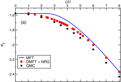
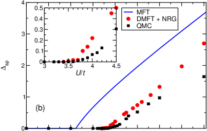
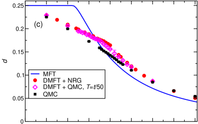
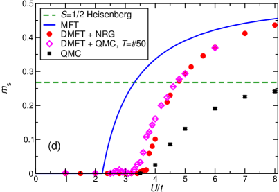
Figure 2: Ground-state energy per site $e_{0}$ (a), single-particle gap $\Delta_{\rm sp}$ (b), double occupancy $d$ (c), and staggered magnetization $m_{\rm s}$ (d) of an infinite honeycomb lattice.

III Static properties

Figure 2 presents a comparison of static quantities that is similar in spirit to the QMC versus MFT comparison of Ref. Feldner et al. (2010); *FeldnerE for an $N=162$ site system subject to periodic boundary conditions, except that it is now for an infinite system and includes the single-site DMFT in the comparison. QMC results are partially taken from Ref. Assaad and Herbut (2013), supplemented by additional data points in order to cover a broader range and new data for the energy (not considered in Ref. Assaad and Herbut (2013)). For our purposes, a system with $18\times 18$ primitive cells, i.e., $N=648$ sites can usually be considered as representative of the thermodynamic limit. For the DMFT, we focus on results obtained with a fast NRG impurity solver, but include results obtained from a slower QMC impurity solver for two quantities in Fig. 2 in order to assess the effect of the different approximations in the impurity solver on top of the DMFT approximation.

The fact that total energies per site $e_{0}$ agree well (Fig. 2(a)) is a prerequisite for also more sensitive quantities to be in good agreement. Still, one can already see that the inclusion of charge fluctuations in DMFT improves over the static MFT, in particular for small to intermediate values of $U$ (for large values of $U$, DMFT approaches again the static MFT result). In addition, one may observe that the MFT result for $e_{0}$ based on the Hamiltonian (4–4) starts to deviate from its $U=0$ value only for $U>U_{c,{\rm MFT}}$ (actually, $U_{c,{\rm MFT}}\approx 2.23\,t$ Sorella and Tosatti (1992) is more clearly identified in other quantities to be discussed below). The same behavior is observed also in other quantities and can be traced to the densities being pinned at $\langle n_{i,\sigma}\rangle=\frac{1}{2}$ for $U<U_{c,{\rm MFT}}$ on the infinite honeycomb lattice.

Next we turn to the staggered magnetization $m_{\rm s}$ shown in Fig. 2(d). The QMC results shown here differ from those of Ref. Assaad and Herbut (2013) in so far as they were computed directly from the $\boldsymbol{Q}=(0,0)$ spin structure factor:

$$S_{\textrm{AF}} = \frac{1}{L^{2}}\sum_{\alpha}\sum_{\boldsymbol{r}}\langle\boldsymbol{S}_{\alpha}(\boldsymbol{r})\cdot\boldsymbol{S}_{\alpha}\rangle,$$

$$m_{\rm s} = \sqrt{\frac{S_{\textrm{AF}}}{N}},$$ (22)

rather than with the aid of a pinning field. The numerical accuracy of NRG being limited by the logarithmic discretization of the frequency axis, values of $m_{\rm s}\lesssim 0.01$ can be considered to be zero within DMFT+NRG. Consequently, in the DMFT+NRG data, we observe a rapid increase of $m_{\rm s}$ around $U/t\approx 3.7$, signaling the onset of magnetism. Thus, we find that the inclusion of charge fluctuations in the DMFT shifts the transition from $U_{c,{\rm MFT}}/t\approx 2.23$ Sorella and Tosatti (1992) much closer to the “exact” QMC result $U_{c}/t\approx 3.78$ Assaad and Herbut (2013). Figure 2(d) also shows data obtained from DMFT+QMC. QMC differs from NRG in that it works on the imaginary frequency axis and at finite temperature (the present data has been obtained at $T=t/50$). Thus, we can compare the effect in particular of finite temperature within QMC and the effect of discretization and broadening of the real-frequency spectral functions in NRG. First, we observe overall good agreement with the biggest differences arising in the critical region. Since it is difficult to say which DMFT variant is more reliable, we conclude from the comparison that the critical point may shift down to $U_{c}/t\approx 3.5$ within DMFT. Despite this uncertainty within DMFT, the value obtained by DMFT is in any case much closer to the “exact” QMC result than static mean-field theory. This good correspondence extends even a bit into the magnetic phase owing to the fact that the mean-field critical exponent $\beta=1$ for the staggered magnetization (also valid for DMFT) is close to the true value $\beta=0.8$ Assaad and Herbut (2013), i.e., the main difference just beyond the critical point seems to be a larger prefactor for DMFT. This is also evident deep inside the magnetic phase. Again, since DMFT is a mean-field theory, it yields $\lim_{U/t\to\infty}m_{\rm s}=1/2$. On the other hand, for $U\gg t$, the half-filled Hubbard model maps onto the spin-1/2 Heisenberg model on the same lattice. The staggered magnetization of the spin-1/2 Heisenberg model is reduced by quantum fluctuations and has been intensively studied for the honeycomb lattice by a broad range of methods Reger et al. (1989); Weihong et al. (1991); Oitmaa et al. (1992); Krüger et al. (2000); Richter et al. (2004); Castro et al. (2006); Jiang et al. (2008a). Figure 2(d) shows the estimate $m_{\rm s}=0.2677(6)$ Castro et al. (2006) for the spin-1/2 Heisenberg model as a dashed horizontal line. The QMC results for the full Hubbard model remain indeed systematically below this line and might approach it asymptotically in the large-$U$ limit.

Now we briefly comment on the single-particle gap that is one half the charge gap, $\Delta_{\rm sp}=(E_{N-1}-2\,E_{N}+E_{N+1})/2$, where $E_{n}$ is the ground-state energy in the sector with $n$ electrons. The single-particle gap $\Delta_{\rm sp}$ is shown in Fig. 2(b); it opens in the magnetic phase and thus exhibits similar behavior as the staggered magnetization. This is particularly evident in the MFT theory where $\Delta_{\rm sp}$ and $m_{\rm s}$ are directly related by Eq. (9). The DMFT+NRG result in Fig. 2(b) is remarkably close to the “exact” lattice QMC and just overestimates the gap a bit. The simple static MFT is again less accurate, as is expected in view of it underestimating the critical value $U_{c}$.

Finally, Fig. 2(c) shows the double occupancy

$$d=\frac{1}{N}\sum_{i}\left\langle n_{i,\uparrow}\,n_{i,\downarrow}\right\rangle\,.$$ (23)

The double occupancy has the advantage that it is related to the magnetic behavior of the system while being more easily accessible by QMC than spin expectation values. The actual QMC data shown in Fig. 2(c) is for $N=648$, but finite-size effects are negligible. We observe first that all three methods yield quantitatively similar results. The MFT transition $U_{c,{\rm MFT}}$ can be detected as the point where the double occupancy starts to fall below the $U=0$ value $d=1/4$, but MFT misses the emergence of a local moment in the paramagnetic phase as signaled by a drop in $d$. This reduction of the double occupancy and the resulting emergence of a local moment are much better reproduced by DMFT that yields results that are significantly closer to the “exact” QMC result for the Hubbard model than plain MFT, i.e., inclusion of local charge fluctuations yields a substantial quantitative improvement. Figure 2(c) compares again the NRG and QMC variants of DMFT. In this case, the difference between the two impurity solvers is found to be very small. However, there is no clear signal of the magnetic transition in $d$, neither in the DMFT nor in the lattice QMC results, i.e., the double occupancy is not very useful for locating the transition point.

Overall, we find that DMFT improves static properties in the semi-metallic phase by including local charge fluctuations beyond static MFT. Specifically, these fluctuations affect the ground-state energy (Fig. 2(a)) and double occupancy (Fig. 2(c)), and shift these quantities close to the “exact” QMC results while within MFT these quantities remain pinned at their non-interacting $U=0$ values throughout the paramagnetic semi-metallic phase. Even the estimate for the critical $U_{c}$ turns out to be remarkably accurate within DMFT. Just deeper in the magnetic phase one observes larger deviations between DMFT and QMC. In particular, DMFT fails to account for the reduction of the magnetic moment at large $U/t$ by quantum fluctuations (see Fig. 2(d)) that would require a proper treatment of their spatial nature. Still, DMFT, in particular in the DMFT+NRG incarnation appears to be a remarkably accurate tool for describing the semi-metallic phase up to the region around $U_{c}$.

IV Spectral functions

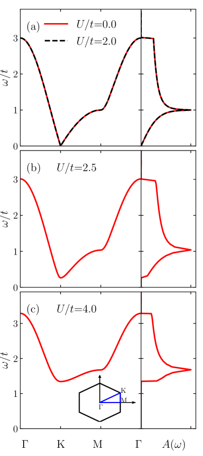
Figure 3: Mean-field result for the single-particle dispersion (left) and local spectral function $A(\omega)$ for $U/t=0$, $2$ (a), $2.5$ (b), and $4$ (c).

IV.1 Static mean-field theory (MFT)

First, we discuss the MFT results for the single-particle spectral functions. Within MFT, the retarded Green’s function reads:

$$G^{\text{ret}}_{\sigma}(\boldsymbol{k},\omega)=\frac{1}{\omega+i0^{+}-\left(\tau_{x}\text{Re}z(\boldsymbol{k})+\tau_{y}\text{Im}z(\boldsymbol{k})-U\,\sigma\,m_{\rm s}\,\tau_{z}\right)}$$ (24)

such that the spin-averaged single-particle spectral function becomes:

$$A(\boldsymbol{k},\omega) = -\text{Im}\sum_{\sigma}\text{Tr}G^{\text{ret}}_{\sigma}(\boldsymbol{k},\omega)$$ (25)

$$= 2\pi\left[\delta(E(\boldsymbol{k})-\omega)+\delta(E(\boldsymbol{k})+\omega)\right]\,.$$

Thus, within MFT the spectral functions consists of $\delta$-functions at the single-particle energy $\pm E(\boldsymbol{k})$. The left column of Fig. 3 shows the mean-field single-particle dispersion Eq. (8). The spectra are reflection symmetric $A(\boldsymbol{k},\omega)=A(\boldsymbol{k},-\omega)$ thanks to the particle-hole symmetry Scalettar (2016); Wakabayashi (2013) and the two sites in the primitive cell of the one-band Hubbard model on the honeycomb lattice. Therefore, here and below we only show positive frequencies $\omega\geq 0$.

Since the matrix elements of the spin-averaged spectral function are constant, see Eq. (25), the local density of states (or local spectral function) $A(\omega)$ is obtained by simple $\boldsymbol{k}$-integration of the MFT dispersion. The result is shown by the right column of Fig. 3.

We observe in panel Fig. 3(a) that at the mean-field level and in the semi-metallic phase $U<U_{c,{\rm MFT}}$, the Coulomb interaction $U$ has no effect on these observables since the mean field vanishes identically (compare a similar remark made for static observables in Sec. III). Consequently, we recover both the well-known dispersion and density of states of non-interacting tight-binding electrons on the honeycomb lattice, see, e.g., Refs. Castro Neto et al. (2009); Castro Neto (2012); Wakabayashi (2013). On the other hand, for $U>U_{c,{\rm MFT}}$, one observes first the opening of a gap at the K point (compare the examples for $U/t=2.5$ and $4$ in Fig. 3(b,c)), an increase of the total bandwidth, and a shift of the sharp peak in the middle of the spectra to higher values of the frequency $\omega$, in accordance with Eq. (8).

IV.2 Dynamical mean-field theory (DMFT)

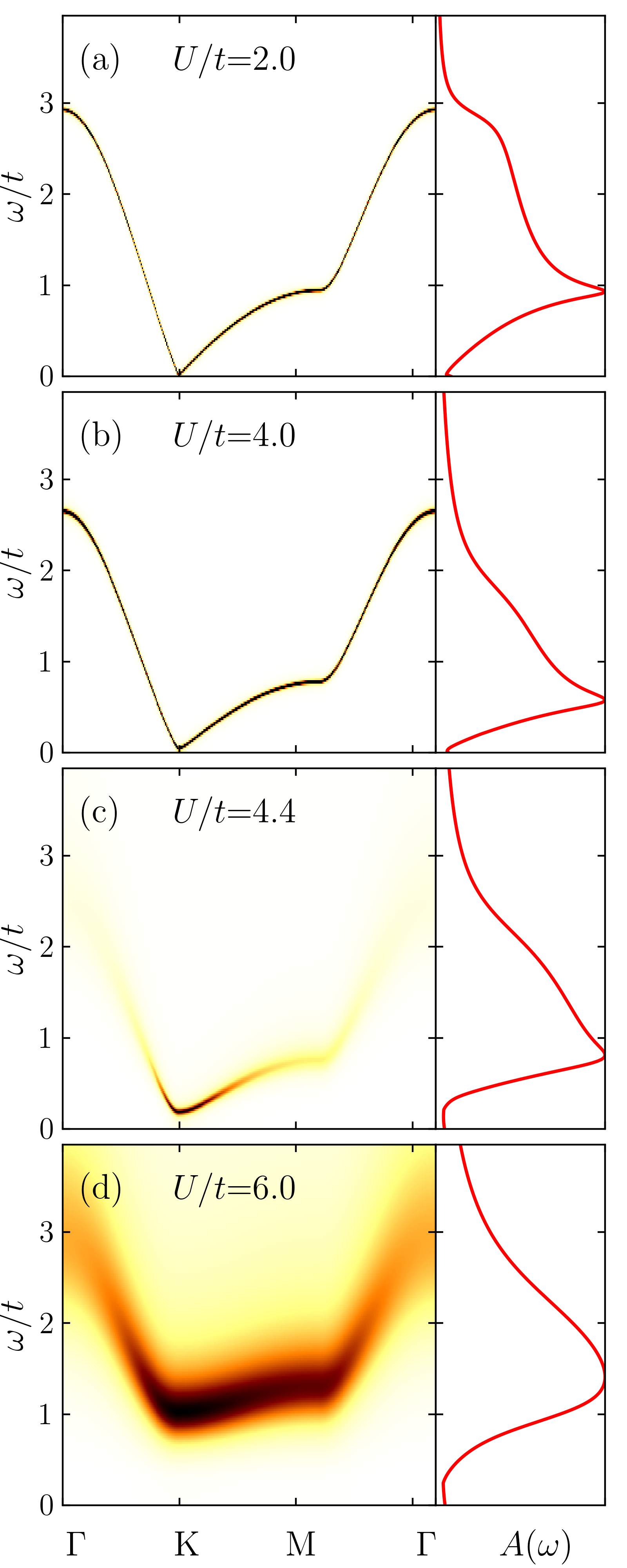
Figure 4: DMFT result for the spectral function $A(\boldsymbol{k},\omega)$ (left) and local spectral function $A(\omega)$ for $U/t=2$, $4$, $4.4$, and $6$ (top to bottom).

Figure 4 shows DMFT results obtained with the NRG impurity solver for the $\boldsymbol{k}$-resolved and local spectral function. In the left column of Fig. 4, we use a color coding to indicate the spectral weight of $A(\boldsymbol{k},\omega)$. Although the non-vanishing self energy $\mathbf{\Sigma}$ does modify the spectral functions also in the semi-metallic phase $0<U<U_{c}$, this effect remains small. This is illustrated by the case $U/t=2$ in Fig. 4(a) that is very similar to the $U=0$ case, see Fig. 3(a). The main difference is a small reduction in bandwidth (see $\omega/t\lesssim 3$) although we recall that the resolution of NRG at these high energies is limited.

The case $U=4\,t$ shown in Fig. 4(b) is already in the antiferromagnetic phase. Consequently, there should be a gap in the spectrum (compare also Fig. 2(b)), but it is too small to be visible in Fig. 4(b). In DMFT, the magnetization and the correlations inherent in the system are still comparably small for $U/t=4$. Thus, the gap due to antiferromagnetic order is small. Furthermore the broadening due to an imaginary part of the self energy is small; the lifetime of the quasiparticles is very long. However, upon increasing the interaction strength to $U/t=4.4$ (Fig. 4(c)), the gap as well as the broadening of the quasiparticle bands become visible. For $U/t=6$ (Fig. 4(d)), the lifetime of the particle becomes short and the bands are strongly broadened due to the self energy. Furthermore, because of Hubbard satellites at $E=\pm U/2$ the bandwidth becomes enhanced.

From the symmetry point of view, the DMFT approximation explicitly breaks the SU(2) spin symmetry. This explicit versus spontaneous symmetry breaking has for consequence that spatial spin fluctuations encoded in the Goldstone modes are absent. As such the DMFT spectral function should be understood in terms of a particle propagating in a frozen antiferromagnetic environment, as in the static mean-field approximation. In fact and from the weak to intermediate coupling limit, the DMFT results presented in Fig. 4 exhibit a spectral function very similar to the mean-field approximation albeit with a broadening due to the imaginary part of the self energy that becomes significant for $U/t=4.4$ and $6$, compare Fig. 4(c,d).

IV.3 Lattice QMC

In the lattice QMC approach the SU(2) spin symmetry is spontaneously broken. As mentioned above this gives rise to collective spin-wave excitations (Goldstone modes) that, as we will see, have a big impact on the single-particle spectral function. Our results are plotted in Fig. 5 across the metal-insulator transition. In the weak-coupling limit, $U/t=2$, the data shown in Fig. 5(a) agrees within numerical accuracy with the DMFT result of Fig. 4(a) and consequently also with the one from static MFT.

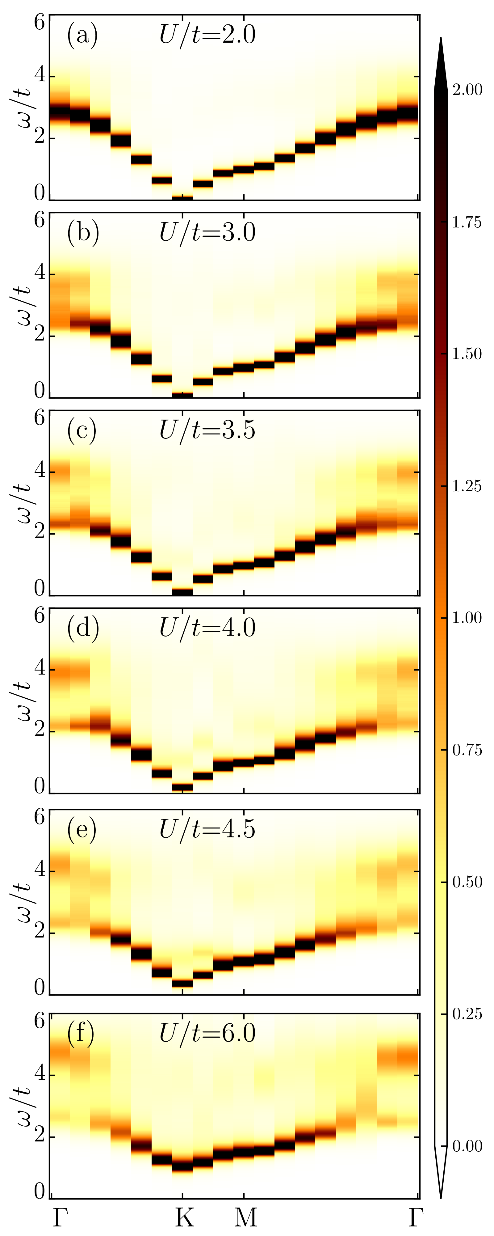
Figure 5: QMC result for the spectral function $A(\boldsymbol{k},\omega)$ on a honeycomb lattice of $18\times 18$ primitive cells.

As appropriate for the Gross-Neveu transition at $U_{c}$, the velocity remains finite, and to a first approximation the opening of the gap follows the mean-field form. The mean-field approximation becomes exact at the upper critical dimension corresponding to $d=3$. By contrast, in two spatial dimensions the single-particle propagator acquires an anomalous dimension, and we would expect a branch cut instead of a pole at the critical point. Within the $\epsilon$-expansion around $d=3$ and at first order Herbut et al. (2009), the fermion anomalous dimension is given by $\eta_{f}=0.03$. This small value is consistent with the fact that we do not observe a broadening of the spectral function in the vicinity of the critical coupling (Fig. 5(c,d)) and at the Dirac point K. We note that this is very similar to the order-disorder transition as realized by the Heisenberg model on a bilayer lattice. Here the anomalous dimension of the bosonic model is equally very small, such that even at the critical point we observe a sharp feature in the dynamical spin structure factor Lohöfer et al. (2015).

Beyond the critical coupling $U_{c}/t\approx 3.78$ Assaad and Herbut (2013), the data for the spectral function corresponds to the motion of a single hole in a quantum antiferromagnet. In conjunction with the cuprates, this problem has been extensively studied on the square lattice Preuss et al. (1995); Martinez and Horsch (1991); Brunner et al. (2000). On the honeycomb lattice, the spectral function shows two prominent features that are especially visible at the $\Gamma$ point starting from $U/t=3.5$ (Fig. 5(c)). First, there is an incoherent high-energy feature that shifts to higher energies with increasing $U/t$. The second low-energy feature for $\omega/t\lesssim 2$ is much sharper. We therefore interpret it as a coherent quasiparticle band, the width of which decreases with increasing $U/t$. As in the $t$-$J$ model on the square lattice Martinez and Horsch (1991); Brunner et al. (2000), one expects the bandwidth of this coherent band to scale as the magnetic scale $J\simeq t^{2}/U$ reflecting the fact that hole motion scrambles the spin background and that the healing procedure can only occur on a time scale set by $J$. We will hence adopt the same terminology as on the square lattice and refer to the coherent feature as the “spin polaron”.

The generic form of the zero-temperature spectral function in the Lehmann representation reads $A_{\sigma}(\boldsymbol{k},\omega)=\pi\sum_{n}|\langle n|c^{\dagger}_{\boldsymbol{k},\sigma}|0\rangle|^{2}\,\delta(E_{n}-E_{0}-\omega)+\pi\sum_{n}|\langle n|c_{\boldsymbol{k},\sigma}|0\rangle|^{2}\,\delta(E_{0}-E_{n}-\omega)$. Here $H|n\rangle=E_{n}|n\rangle$ and the sum rule $\int{\rm d}\omega\,A_{\sigma}(\boldsymbol{k},\omega)=\pi$ holds. Hence both the energy spectrum and the matrix elements are required for a full understanding of the spectral function. In particular the support of the spectral function is given by the energy spectrum and the distribution of weight by the matrix elements. At our largest coupling, $U/t=6$, it is apparent from Fig. 5(f) that at the $\Gamma$ point the dominant weight is in the incoherent high-energy feature and that this spectral weight is transferred to the coherent spin-polaron band upon approaching the M or K point. This rather abrupt transfer of spectral weight is referred to as waterfall in the high-$T_{c}$ literature and has been observed in simulations of the Hubbard model on the square lattice Preuss et al. (1995); Moritz et al. (2010) as well as experimentally in photoemission studies of the cuprates Graf et al. (2007).

V Conclusions and discussion

We have performed a comparative investigation of the one-band Hubbard model on the honeycomb lattice, using static mean-field theory (MFT), dynamical mean-field theory (DMFT), and “exact” quantum Monte Carlo (QMC) simulations on the lattice. All three methods yield a semi-metallic Dirac phase and an antiferromagnetic insulator. The critical point in MFT $U_{c,{\rm MFT}}\approx 2.23\,t$ Sorella and Tosatti (1992) is significantly below the exact location $U_{c}/t\approx 3.78$ Assaad and Herbut (2013). Our first finding is that the single-site DMFT yields a very good approximation to this value, namely $3.5\lesssim U_{c}/t\lesssim 3.7$ and is thus competitive in accuracy with more sophisticated generalizations of DMFT Wu and Tremblay (2014); Hirschmeier et al. (2018). In this respect, an accurate treatment of the effective impurity problem thus appears to be more important than going to big cluster sizes.

Within static MFT, all quantities are independent of $U$ for $U<U_{c}$ owing to the vanishing mean field. This is improved by DMFT, yielding in particular more accurate values of the ground-state energy and double occupancy. All three methods find qualitatively similar spectral functions in the semi-metallic phase with a sharp and gapless quasiparticle. The main improvement by DMFT in this case is a broader range in $U$ that is accessible owing to the better estimate for $U_{c}$. Overall, we find that single-site DMFT provides a remarkably accurate description of the weakly correlated semi-metallic phase at a low computational cost, in particular when the numerical renormalization group (NRG) Wilson (1975); Bulla et al. (2008) is used as impurity solver.

Both simple MFT and DMFT yield mean-field critical behavior and are thus not expected to provide quantitatively accurate results close to $U_{c}$ and in particular for the critical exponents although the actual values for the relevant Gross-Neveu transition are quite close to the mean-field values Assaad and Herbut (2013); Herbut et al. (2009). For large values of $U$ deep inside the antiferromagnetic phase, DMFT reduces again to static MFT and misses in particular the non-local spin fluctuations. Thus, the staggered magnetization $m_{\rm s}$ tends to $1/2$ for $U\to\infty$ both within static MFT and DMFT, i.e., both methods fail to reproduce the reduction of the ordered moment at large $U$ by quantum fluctuations. For the same reasons, DMFT and in particular MFT overestimate the single-particle gap that is induced by the magnetic order in the magnetic phase.

As a first perspective for further work, we mention applications to magnetism induced at zig-zag edges of graphene-type nanostructures Yazyev (2010); Wakabayashi (2013); Fujita et al. (1996); Wakabayashi et al. (1998); Fernández-Rossier and Palacios (2007); Bhowmick and Shenoy (2008); Jiang et al. (2008b); Viana-Gomes et al. (2009); Feldner et al. (2010); *FeldnerE; Feldner et al. (2011); Roy et al. (2014); Valli et al. (2016); Raczkowski and Assaad (2017). Previous studies Feldner et al. (2010); *FeldnerE; Feldner et al. (2011) observed that simple MFT is remarkably successful in describing at least some aspects of this phenomenon in the weakly correlated regime. In particular, the local spectral functions for nanoribbons turned out to be remarkably accurate in MFT Feldner et al. (2011). The main shortcoming of MFT is that it underestimates the bulk critical value of $U_{c}$, thus limiting the range of $U$ where MFT applies. It is straightforward to generalize the single-site DMFT employed in the present work to real-space nanostructures in the same way as static MFT. Since our single-site DMFT yields a much better estimate for $U_{c}$, we speculate that a real-space variant will also further improve the description of edge-state magnetism beyond static MFT, at least in the weakly correlated regime relevant to graphene, despite the shortcomings of the single-site DMFT in the magnetic phase.

One of the biggest challenges in realistic DMFT-based calculations is to include non-local correlations Vollhardt and Lichtenstein (2017). We believe that this work provides a non-trivial benchmark to further test various schemes aimed at including non-local fluctuations around the DMFT solution. This includes dual fermions Rubtsov et al. (2008), the dynamical vertex approximation Toschi et al. (2007), as well as extended DMFT Smith and Si (2000). On the other hand one can start with implementations of the functional renormalization group Metzner et al. (2012) approach that captures spatial correlations but neglects temporal ones. Irrespective of the starting point, the proposed benchmark is highly non-trivial since the critical point is Lorentz invariant such that long-wave-length fluctuations in space and time are identical.

*

Appendix A Structure of the self energy

The symmetry differences between the QMC simulations and the DMFT approximation become evident when considering the self energy. The QMC simulations possess the full symmetry of the Hubbard model: SU(2) spin rotation, inversion, time reversal, as well as particle-hole symmetries.

Particle-hole symmetry, $\hat{P}$, is an anti-linear transformation that maps:

$$\hat{P}^{-1}\alpha\begin{pmatrix}c_{A,\sigma}(\boldsymbol{k})\\ c_{B,\sigma}(\boldsymbol{k})\end{pmatrix}\hat{P}^{-1}=\overline{\alpha}\begin{pmatrix}c^{\dagger}_{A,-\sigma}(\boldsymbol{k})\\ -c^{\dagger}_{B,-\sigma}(\boldsymbol{k})\end{pmatrix}$$

$$=\overline{\alpha}\tau_{z}\begin{pmatrix}c^{\dagger}_{A,-\sigma}(\boldsymbol{k})\\ c^{\dagger}_{B,-\sigma}(\boldsymbol{k})\end{pmatrix}.$$ (26)

Due to the SU(2) spin symmetry, the single-particle Green’s function matrix is spin independent and satisfies the symmetry property:

$$\boldsymbol{G}^{\text{ret}}(\boldsymbol{k},\omega)=-\tau_{z}\,\boldsymbol{G}^{\text{ret}}(\boldsymbol{k},-\omega)\,\tau_{z}.$$ (27)

Inversion symmetry amounts to:

$$\hat{I}^{-1}\begin{pmatrix}c_{A,\sigma}(\boldsymbol{k})\\ c_{B,\sigma}(\boldsymbol{k})\end{pmatrix}\hat{I}=\begin{pmatrix}c_{B,\sigma}(-\boldsymbol{k})\\ c_{A,\sigma}(-\boldsymbol{k})\end{pmatrix}=\tau_{x}\,\begin{pmatrix}c_{A,\sigma}(-\boldsymbol{k})\\ c_{B,\sigma}(-\boldsymbol{k})\end{pmatrix}$$ (28)

and as a consequence,

$$\boldsymbol{G}^{\text{ret}}(\boldsymbol{k},\omega)=\tau_{x}\,\boldsymbol{G}^{\text{ret}}(-\boldsymbol{k},\omega)\,\tau_{x}\,.$$ (29)

Finally, time reversal symmetry reads:

$$\hat{T}^{-1}\alpha\begin{pmatrix}c_{A,\sigma}(\boldsymbol{k})\\ c_{B,\sigma}(\boldsymbol{k})\end{pmatrix}\hat{T}=\overline{\alpha}\sum_{s}(i\sigma_{y})_{\sigma,s}\begin{pmatrix}c_{A,s}(-\boldsymbol{k})\\ c_{B,s}(-\boldsymbol{k})\end{pmatrix}$$ (30)

leading to

$$\boldsymbol{G}^{\text{ret}}(\boldsymbol{k},\omega)=\boldsymbol{G}^{\text{adv}}(-\boldsymbol{k},\omega)\,.$$ (31)

One will readily check that the non-interacting Green’s function of Eq. (24) at $m_{\rm s}=0$ satisfies all the above properties.

Owing to the Dyson equation, the aforementioned symmetries carry over to the self-energy matrix that has to satisfy:

$$\boldsymbol{\Sigma}(\boldsymbol{k},\omega)=\tau_{x}\,\boldsymbol{\Sigma}(-\boldsymbol{k},\omega)\,\tau_{x}\,,$$ (32)

$$\boldsymbol{\Sigma}(\boldsymbol{k},\omega)=-\tau_{z}\,\boldsymbol{\Sigma}(\boldsymbol{k},-\omega)\,\tau_{z}\,,$$ (33)

Let us now parameterize the self energy as

$$\boldsymbol{\Sigma}(\boldsymbol{k},\omega)=\Sigma_{x}(\boldsymbol{k},\omega)\,\tau_{x}+\Sigma_{y}(\boldsymbol{k},\omega)\,\tau_{y}+\Sigma_{z}(\boldsymbol{k},\omega)\,\tau_{z}+\Sigma_{0}(\boldsymbol{k},\omega)$$ (34)

where $\Sigma_{\alpha}(\boldsymbol{k},\omega)$ are scalar functions. Inversion and particle-hole symmetry then implies that:

$$\Sigma_{x}(\boldsymbol{k},\omega)=\phantom{-}\Sigma_{x}(-\boldsymbol{k},\omega)=\phantom{-}\Sigma_{x}(\boldsymbol{k},-\omega)$$

$$\Sigma_{y}(\boldsymbol{k},\omega)=-\Sigma_{y}(-\boldsymbol{k},\omega)=\phantom{-}\Sigma_{y}(\boldsymbol{k},-\omega)$$

$$\Sigma_{z}(\boldsymbol{k},\omega)=-\Sigma_{z}(-\boldsymbol{k},\omega)=-\Sigma_{z}(\boldsymbol{k},-\omega)$$

$$\Sigma_{0}(\boldsymbol{k},\omega)=\phantom{-}\Sigma_{0}(-\boldsymbol{k},\omega)=-\Sigma_{0}(\boldsymbol{k},-\omega)\,.$$ (35)

Generically, one sees that $\Sigma_{0}$ and $\Sigma_{z}$ are odd functions of frequency whereas $\Sigma_{x}$ and $\Sigma_{y}$ are even functions of frequency. The above greatly simplifies at time-reversal symmetric points in the Brillouin zone, $\overline{\boldsymbol{k}}=\Gamma$, M. Here the self energy reads:

$$\boldsymbol{\Sigma}(\overline{\boldsymbol{k}},\omega)=\tau_{x}\Sigma_{x}(\overline{\boldsymbol{k}},\omega)+\Sigma_{0}(\overline{\boldsymbol{k}},\omega).$$ (36)

This stands in strong contrast to the single-site DMFT approximation where the self energy is spin dependent and diagonal in orbital space:

$$\boldsymbol{\Sigma}^{\rm DMFT}_{\sigma}(\omega)=\sigma\,\tau_{z}\,\Sigma^{\rm DMFT}(\omega).$$ (37)

We note that the DMFT self energy satisfies particle-hole symmetry but violates inversion as well as time reversal.

Returning to the QMC simulations, we have the following relation at the $\Gamma$ point:

$$\text{Tr}\,\boldsymbol{G}^{\text{ret}}(\Gamma,\omega) = \frac{2(\omega-\Sigma_{0}(\Gamma,\omega))}{(\omega+i0^{+}-\Sigma_{0}(\Gamma,\omega))^{2}-(3+\Sigma_{x}(\Gamma,\omega))^{2}}\,.$$

In contrast for the DMFT calculation we obtain:

$$\text{Tr}\,\boldsymbol{G}_{\sigma}^{\text{ret},DMFT}(\Gamma,\omega) = \frac{2\omega}{(\omega+i0^{+})^{2}-(\Sigma^{DMFT}(\Gamma,\omega))^{2}-9}\,.$$

Hence we can certainly compare the spectral functions, but comparison of the self energy seems difficult.

References

- Hubbard (1963) J. Hubbard, “Electron correlations in narrow energy bands,” Proc. R. Soc. London, Ser. A 276, 238–257 (1963).
- Kanamori (1963) Junjiro Kanamori, “Electron correlation and ferromagnetism of transition metals,” Progr. Theor. Phys. 30, 275–289 (1963).
- Gutzwiller (1963) Martin C. Gutzwiller, “Effect of correlation on the ferromagnetism of transition metals,” Phys. Rev. Lett. 10, 159–162 (1963).
- Tasaki (1998) Hal Tasaki, “The Hubbard model – an introduction and selected rigorous results,” J. Phys.: Condens. Matter 10, 4353–4378 (1998).
- Eder (2017) Robert Eder, “Introduction to the Hubbard model,” in The Physics of Correlated Insulators, Metals, and Superconductors, Modeling and Simulation, Vol. 7 (Forschungszentrum Jülich, Jülich, 2017) pp. 6.1–6.29.
- Dagotto (1994) Elbio Dagotto, “Correlated electrons in high-temperature superconductors,” Rev. Mod. Phys. 66, 763–840 (1994).
- Brenig (1995) Wolfram Brenig, “Aspects of electron correlations in the cuprate superconductors,” Phys. Rep. 251, 153–266 (1995).
- Preuss et al. (1995) R. Preuss, W. Hanke, and W. von der Linden, “Quasiparticle dispersion of the 2D Hubbard model: From an insulator to a metal,” Phys. Rev. Lett. 75, 1344–1347 (1995).
- Preuss et al. (1997) R. Preuss, W. Hanke, C. Gröber, and H. G. Evertz, “Pseudogaps and their interplay with magnetic excitations in the doped 2D Hubbard model,” Phys. Rev. Lett. 79, 1122–1125 (1997).
- Brunner et al. (2000) Michael Brunner, Fakher F. Assaad, and Alejandro Muramatsu, “Single-hole dynamics in the model on a square lattice,” Phys. Rev. B 62, 15480–15492 (2000).
- Kyung et al. (2006) B. Kyung, S. S. Kancharla, D. Sénéchal, A.-M. S. Tremblay, M. Civelli, and G. Kotliar, “Pseudogap induced by short-range spin correlations in a doped Mott insulator,” Phys. Rev. B 73, 165114 (2006).
- Macridin et al. (2007) Alexandru Macridin, M. Jarrell, Thomas Maier, and D. J. Scalapino, “High-energy kink in the single-particle spectra of the two-dimensional Hubbard model,” Phys. Rev. Lett. 99, 237001 (2007).
- Zemljič et al. (2008) M. M. Zemljič, P. Prelovšek, and T. Tohyama, “Temperature and doping dependence of the high-energy kink in cuprates,” Phys. Rev. Lett. 100, 036402 (2008).
- Wróbel et al. (2008) P. Wróbel, W. Suleja, and R. Eder, “Spin-polaron band structure and hole pockets in underdoped cuprates,” Phys. Rev. B 78, 064501 (2008).
- Moritz et al. (2010) B. Moritz, S. Johnston, and T. P. Devereaux, “Insights on the cuprate high energy anomaly observed in ARPES,” Journal of Electron Spectroscopy and Related Phenomena 181, 31–34 (2010).
- Sakai et al. (2010) Shiro Sakai, Yukitoshi Motome, and Masatoshi Imada, “Doped high- cuprate superconductors elucidated in the light of zeros and poles of the electronic Green’s function,” Phys. Rev. B 82, 134505 (2010).
- Dalla Piazza et al. (2012) B. Dalla Piazza, M. Mourigal, M. Guarise, H. Berger, T. Schmitt, K. J. Zhou, M. Grioni, and H. M. Rønnow, “Unified one-band Hubbard model for magnetic and electronic spectra of the parent compounds of cuprate superconductors,” Phys. Rev. B 85, 100508 (2012).
- Rost et al. (2012) D. Rost, E. V. Gorelik, F. Assaad, and N. Blümer, “Momentum-dependent pseudogaps in the half-filled two-dimensional Hubbard model,” Phys. Rev. B 86, 155109 (2012).
- Kohno (2014) Masanori Kohno, “Spectral properties near the Mott transition in the two-dimensional Hubbard model with next-nearest-neighbor hopping,” Phys. Rev. B 90, 035111 (2014).
- Yang and Feiguin (2016) Chun Yang and Adrian E. Feiguin, “Spectral function of the two-dimensional Hubbard model: A density matrix renormalization group plus cluster perturbation theory study,” Phys. Rev. B 93, 081107 (2016).
- Wang et al. (2018) Yao Wang, Brian Moritz, Cheng-Chien Chen, Thomas P. Devereaux, and Krzysztof Wohlfeld, “Influence of magnetism and correlation on the spectral properties of doped Mott insulators,” Phys. Rev. B 97, 115120 (2018).
- Hirsch (1985) J. E. Hirsch, “Two-dimensional Hubbard model: Numerical simulation study,” Phys. Rev. B 31, 4403–4419 (1985).
- White et al. (1989) S. White, D. Scalapino, R. Sugar, E. Loh, J. Gubernatis, and R. Scalettar, “Numerical study of the two-dimensional Hubbard model,” Phys. Rev. B 40, 506–516 (1989).
- Sorella and Tosatti (1992) S. Sorella and E. Tosatti, “Semi-metal-insulator transition of the Hubbard model in the honeycomb lattice,” Europhys. Lett. 19, 699–704 (1992).
- Geim and Novoselov (2007) A. K. Geim and K. S. Novoselov, “The rise of graphene,” Nature Materials 6, 183–191 (2007).
- Castro Neto et al. (2009) A. H. Castro Neto, F. Guinea, N. M. R. Peres, K. S. Novoselov, and A. K. Geim, “The electronic properties of graphene,” Rev. Mod. Phys. 81, 109–162 (2009).
- Yazyev (2010) Oleg V. Yazyev, “Emergence of magnetism in graphene materials and nanostructures,” Rep. Prog. Phys. 73, 056501 (2010).
- Wakabayashi (2013) Katsunori Wakabayashi, “Electronic properties of nanographene,” in Physics and Chemistry of Graphene, edited by T. Enoki and T. Ando (Pan Stanford, New York, 2013) Chap. 4, pp. 207–288.
- Meng et al. (2010) Z. Y. Meng, T. C. Lang, S. Wessel, F. F. Assaad, and A. Muramatsu, “Quantum spin liquid emerging in two-dimensional correlated Dirac fermions,” Nature 464, 847–851 (2010).
- Sorella et al. (2012) Sandro Sorella, Yuichi Otsuka, and Seiji Yunoki, “Absence of a spin liquid phase in the Hubbard model on the honeycomb lattice,” Scientific Reports 2, 992 (2012).
- He and Lu (2012) Rong-Qiang He and Zhong-Yi Lu, “Cluster dynamical mean field theory of quantum phases on a honeycomb lattice,” Phys. Rev. B 86, 045105 (2012).
- Hassan and Sénéchal (2013) S. R. Hassan and David Sénéchal, “Absence of spin liquid in nonfrustrated correlated systems,” Phys. Rev. Lett. 110, 096402 (2013).
- Seki and Ohta (2013) Kazuhiro Seki and Yukinori Ohta, “Variational cluster approach to the Hubbard model on a honeycomb lattice,” J. Kor. Phys. Soc. 62, 2150–2154 (2013).
- Assaad and Herbut (2013) Fakher F. Assaad and Igor F. Herbut, “Pinning the order: The nature of quantum criticality in the Hubbard model on honeycomb lattice,” Phys. Rev. X 3, 031010 (2013).
- Wu and Tremblay (2014) Wei Wu and A.-M. S. Tremblay, “Phase diagram and Fermi liquid properties of the extended Hubbard model on the honeycomb lattice,” Phys. Rev. B 89, 205128 (2014).
- Herbut et al. (2009) Igor F. Herbut, Vladimir Juričić, and Oskar Vafek, “Relativistic Mott criticality in graphene,” Phys. Rev. B 80, 075432 (2009).
- Ryu et al. (2009) Shinsei Ryu, Christopher Mudry, Chang-Yu Hou, and Claudio Chamon, “Masses in graphenelike two-dimensional electronic systems: Topological defects in order parameters and their fractional exchange statistics,” Phys. Rev. B 80, 205319 (2009).
- Feldner et al. (2010) Hélène Feldner, Zi Yang Meng, Andreas Honecker, Daniel Cabra, Stefan Wessel, and Fakher F. Assaad, “Magnetism of finite graphene samples: Mean-field theory compared with exact diagonalization and quantum Monte Carlo simulations,” Phys. Rev. B 81, 115416 (2010).
- Feldner et al. (2020) Hélène Feldner, Zi Yang Meng, Andreas Honecker, Daniel Cabra, Stefan Wessel, and Fakher F. Assaad, “Erratum: Magnetism of finite graphene samples: Mean-field theory compared with exact diagonalization and quantum Monte Carlo simulations [Phys. Rev. B 81, 115416 (2010)],” Phys. Rev. B 101, 049909 (2020).
- Jafari (2009) S. A. Jafari, “Dynamical mean field study of the Dirac liquid,” Eur. Phys. J. B 68, 537–542 (2009).
- Tran and Kuroki (2009) Minh-Tien Tran and Kazuhiko Kuroki, “Finite-temperature semimetal-insulator transition on the honeycomb lattice,” Phys. Rev. B 79, 125125 (2009).
- Liebsch and Wu (2013) Ansgar Liebsch and Wei Wu, “Coulomb correlations in the honeycomb lattice: Role of translation symmetry,” Phys. Rev. B 87, 205127 (2013).
- Hirschmeier et al. (2018) Daniel Hirschmeier, Hartmut Hafermann, and Alexander I. Lichtenstein, “Multiband dual fermion approach to quantum criticality in the Hubbard honeycomb lattice,” Phys. Rev. B 97, 115150 (2018).
- Scalettar (2016) Richard Scalettar, “An introduction to the Hubbard Hamiltonian,” in Quantum Materials: Experiments and Theory, Modeling and Simulation, Vol. 6 (Forschungszentrum Jülich, Jülich, 2016) pp. 4.1–4.29.
- Georges et al. (1996) Antoine Georges, Gabriel Kotliar, Werner Krauth, and Marcelo J. Rozenberg, “Dynamical mean-field theory of strongly correlated fermion systems and the limit of infinite dimensions,” Rev. Mod. Phys. 68, 13–125 (1996).
- Wilson (1975) Kenneth G. Wilson, “The renormalization group: Critical phenomena and the Kondo problem,” Rev. Mod. Phys. 47, 773–840 (1975).
- Bulla et al. (2008) Ralf Bulla, Theo A. Costi, and Thomas Pruschke, “Numerical renormalization group method for quantum impurity systems,” Rev. Mod. Phys. 80, 395–450 (2008).
- Werner et al. (2006) Philipp Werner, Armin Comanac, Luca de’ Medici, Matthias Troyer, and Andrew J. Millis, “Continuous-time solver for quantum impurity models,” Phys. Rev. Lett. 97, 076405 (2006).
- Gull et al. (2011) Emanuel Gull, Andrew J. Millis, Alexander I. Lichtenstein, Alexey N. Rubtsov, Matthias Troyer, and Philipp Werner, “Continuous-time Monte Carlo methods for quantum impurity models,” Rev. Mod. Phys. 83, 349–404 (2011).
- Hafermann et al. (2013) Hartmut Hafermann, Philipp Werner, and Emanuel Gull, “Efficient implementation of the continuous-time hybridization expansion quantum impurity solver,” Comp. Phys. Commun. 184, 1280–1286 (2013).
- Bauer et al. (2011) B. Bauer, L. D. Carr, H. G. Evertz, A. Feiguin, J. Freire, S. Fuchs, L. Gamper, J. Gukelberger, E. Gull, S. Guertler, A. Hehn, R. Igarashi, S. V. Isakov, D. Koop, P. N. Ma, P. Mates, H. Matsuo, O. Parcollet, G. Pawłowski, J. D. Picon, L. Pollet, E. Santos, V. W. Scarola, U. Schollwöck, C. Silva, B. Surer, S. Todo, S. Trebst, M. Troyer, M. L. Wall, P. Werner, and S. Wessel, “The ALPS project release 2.0: open source software for strongly correlated systems,” Journal of Statistical Mechanics: Theory and Experiment 2011, P05001 (2011).
- Peters et al. (2006) Robert Peters, Thomas Pruschke, and Frithjof B. Anders, “Numerical renormalization group approach to Green’s functions for quantum impurity models,” Phys. Rev. B 74, 245114 (2006).
- Sugiyama and Koonin (1986) G. Sugiyama and S. E. Koonin, “Auxiliary field Monte-Carlo for quantum many-body ground states,” Ann. Phys. (N.Y.) 168, 1–26 (1986).
- Sorella et al. (1989) S. Sorella, S. Baroni, R. Car, and M. Parrinello, “A novel technique for the simulation of interacting fermion systems,” Europhys. Lett. 8, 663 (1989).
- Imada and Hatsugai (1989) Masatoshi Imada and Yasuhiro Hatsugai, “Numerical studies on the Hubbard model and the model in one- and two-dimensions,” J. Phys. Soc. Jpn. 58, 3752–3780 (1989).
- Assaad and Evertz (2008) F. F. Assaad and H. G. Evertz, “World-line and determinantal quantum Monte Carlo methods for spins, phonons and electrons,” in Computational Many-Particle Physics, edited by H. Fehske, R. Schneider, and A. Weiße (Springer Berlin Heidelberg, Berlin, Heidelberg, 2008) pp. 277–356.
- Bercx et al. (2017) Martin Bercx, Florian Goth, Johannes S. Hofmann, and Fakher F. Assaad, “The ALF (Algorithms for Lattice Fermions) project release 1.0. documentation for the auxiliary field quantum Monte Carlo codes,” SciPost Phys. 3, 013 (2017).
- Sandvik (1998) Anders Sandvik, “Stochastic method for analytic continuation of quantum Monte Carlo data,” Phys. Rev. B 57, 10287–10290 (1998).
- Beach (2004) K. S. D. Beach, “Identifying the maximum entropy method as a special limit of stochastic analytic continuation,” eprint arXiv:cond-mat/0403055 (2004), cond-mat/0403055 .
- Reger et al. (1989) J. D. Reger, J. A. Riera, and A. P. Young, “Monte Carlo simulations of the spin- Heisenberg antiferromagnet in two dimensions,” J. Phys.: Condens. Matter 1, 1855–1865 (1989).
- Weihong et al. (1991) Zheng Weihong, J. Oitmaa, and C. J. Hamer, “Second-order spin-wave results for the quantum and models with anisotropy,” Phys. Rev. B 44, 11869–11881 (1991).
- Oitmaa et al. (1992) J. Oitmaa, C. J. Hamer, and Zheng Weihong, “Quantum magnets on the honeycomb and triangular lattices at ,” Phys. Rev. B 45, 9834–9841 (1992).
- Krüger et al. (2000) Sven E. Krüger, Johannes Richter, Jörg Schulenburg, Damian J. J. Farnell, and Raymond F. Bishop, “Quantum phase transitions of a square-lattice Heisenberg antiferromagnet with two kinds of nearest-neighbor bonds: A high-order coupled-cluster treatment,” Phys. Rev. B 61, 14607–14615 (2000).
- Richter et al. (2004) Johannes Richter, Jörg Schulenburg, and Andreas Honecker, “Quantum magnetism in two dimensions: From semi-classical Néel order to magnetic disorder,” Lect. Notes Phys. 645, 85–153 (2004).
- Castro et al. (2006) Eduardo V. Castro, N. M. R. Peres, K. S. D. Beach, and Anders W. Sandvik, “Site dilution of quantum spins in the honeycomb lattice,” Phys. Rev. B 73, 054422 (2006).
- Jiang et al. (2008a) H. C. Jiang, Z. Y. Weng, and T. Xiang, “Accurate determination of tensor network state of quantum lattice models in two dimensions,” Phys. Rev. Lett. 101, 090603 (2008a).
- Castro Neto (2012) Antonio H. Castro Neto, “Selected topics in graphene physics,” Lect. Notes Phys. 843, 117–144 (2012).
- Lohöfer et al. (2015) M. Lohöfer, T. Coletta, D. G. Joshi, F. F. Assaad, M. Vojta, S. Wessel, and F. Mila, “Dynamical structure factors and excitation modes of the bilayer Heisenberg model,” Phys. Rev. B 92, 245137 (2015).
- Martinez and Horsch (1991) Gerardo Martinez and Peter Horsch, “Spin polarons in the - model,” Phys. Rev. B 44, 317–331 (1991).
- Graf et al. (2007) J. Graf, G.-H. Gweon, and A. Lanzara, “Universal waterfall-like feature in the spectral function of high temperature superconductors,” Physica C 460-462, 194–197 (2007).
- Fujita et al. (1996) Mitsutaka Fujita, Katsunori Wakabayashi, Kyoko Nakada, and Koichi Kusakabe, “Peculiar localized state at zigzag graphite edge,” J. Phys. Soc. Jpn. 65, 1920–1923 (1996).
- Wakabayashi et al. (1998) Katsunori Wakabayashi, Manfred Sigrist, and Mitsutaka Fujita, “Spin wave mode of edge-localized magnetic states in nanographite zigzag ribbons,” J. Phys. Soc. Jpn. 67, 2089–2093 (1998).
- Fernández-Rossier and Palacios (2007) J. Fernández-Rossier and J. J. Palacios, “Magnetism in graphene nanoislands,” Phys. Rev. Lett. 99, 177204 (2007).
- Bhowmick and Shenoy (2008) Somnath Bhowmick and Vijay B. Shenoy, “Edge state magnetism of single layer graphene nanostructures,” J. Chem. Phys. 128, 244717 (2008).
- Jiang et al. (2008b) J. Jiang, W. Lu, and J. Bernholc, “Edge states and optical transition energies in carbon nanoribbons,” Phys. Rev. Lett. 101, 246803 (2008b).
- Viana-Gomes et al. (2009) J. Viana-Gomes, Vitor M. Pereira, and N. M. R. Peres, “Magnetism in strained graphene dots,” Phys. Rev. B 80, 245436 (2009).
- Feldner et al. (2011) Hélène Feldner, Zi Yang Meng, Thomas C. Lang, Fakher F. Assaad, Stefan Wessel, and Andreas Honecker, “Dynamical signatures of edge-state magnetism on graphene nanoribbons,” Phys. Rev. Lett. 106, 226401 (2011).
- Roy et al. (2014) Bitan Roy, Fakher F. Assaad, and Igor F. Herbut, “Zero modes and global antiferromagnetism in strained graphene,” Phys. Rev. X 4, 021042 (2014).
- Valli et al. (2016) A. Valli, A. Amaricci, A. Toschi, T. Saha-Dasgupta, K. Held, and M. Capone, “Effective magnetic correlations in hole-doped graphene nanoflakes,” Phys. Rev. B 94, 245146 (2016).
- Raczkowski and Assaad (2017) Marcin Raczkowski and Fakher F. Assaad, “Interplay between the edge-state magnetism and long-range Coulomb interaction in zigzag graphene nanoribbons: Quantum Monte Carlo study,” Phys. Rev. B 96, 115155 (2017).
- Vollhardt and Lichtenstein (2017) D. Vollhardt and A. I. Lichtenstein, “Dynamical mean-field approach with predictive power for strongly correlated materials,” The European Physical Journal Special Topics 226, 2439–2443 (2017).
- Rubtsov et al. (2008) A. N. Rubtsov, M. I. Katsnelson, and A. I. Lichtenstein, “Dual fermion approach to nonlocal correlations in the Hubbard model,” Phys. Rev. B 77, 033101 (2008).
- Toschi et al. (2007) A. Toschi, A. A. Katanin, and K. Held, “Dynamical vertex approximation: A step beyond dynamical mean-field theory,” Phys. Rev. B 75, 045118 (2007).
- Smith and Si (2000) J. Lleweilun Smith and Qimiao Si, “Spatial correlations in dynamical mean-field theory,” Phys. Rev. B 61, 5184–5193 (2000).
- Metzner et al. (2012) Walter Metzner, Manfred Salmhofer, Carsten Honerkamp, Volker Meden, and Kurt Schönhammer, “Functional renormalization group approach to correlated fermion systems,” Rev. Mod. Phys. 84, 299–352 (2012).