Distinct properties of the radio burst emission from the magnetar XTE J1810$-$197

Abstract

XTE J1810$-$197 (PSR J1809$-$1943) was the first ever magnetar which was found to emit transient radio emission. It has recently undergone another radio and high-energy outburst. This is only the second radio outburst that has been observed from this source. We observed J1810$-$197 soon after its recent radio outburst at low radio frequencies using the Giant Metrewave Radio Telescope. We present the 650 MHz flux density evolution of the source in the early phases of the outburst, and its radio spectrum down to frequencies as low as 300 MHz. The magnetar also exhibits radio emission in the form of strong, narrow bursts. We show that the bursts have a characteristic intrinsic width of the order of 0.5$-$0.7 ms, and discuss their properties in the context of giant pulses and giant micropulses from other pulsars. We also show that the bursts exhibit spectral structures which cannot be explained by interstellar propagation effects. These structures might indicate a phenomenological link with the repeating fast radio bursts which also show interesting, more detailed frequency structures. While the spectral structures are particularly noticeable in the early phases of the outburst, these seem to be less prominent as well as less frequent in the later phases, suggesting an evolution of the underlying cause of these spectral structures.

1 Introduction

Magnetars are characterized by their high magnetic fields ($10^{14}-10^{15}$ G), young age, persistent but highly variable X-ray emission, and transient radio emission. Transient radio pulsations have been observed from a handful of magnetars, while no radio emission has been found from others despite deep searches (e.g., Surnis et al., 2016). The anomalous X-ray pulsar XTE J1810$-$197 (PSR J1809$-$1943) was the first magnetar found to be emitting radio pulses (Camilo et al., 2006) after a strong high energy outburst (Gotthelf et al., 2003; Ibrahim et al., 2004). At the beginning of the outburst, a nearly flat spectral index between 0.7$-$42 GHz was reported. The radio flux density decreased along with the X-ray flux with a long decay time, and the source became undetectable in late 2008 (Camilo et al., 2016). Regular radio monitoring of the source revealed its reactivation at 1.5 GHz in late 2018 (Lyne et al., 2018), which was followed by its successful detection at a wide range of radio frequencies (0.65$-$11.7 GHz, e.g., Joshi et al., 2018; Trushkin et al., 2019).

In its previous outburst, J1810$-$197 exhibited spikes or bursts of radio emission with typical widths $\lesssim$10 ms, and structures as narrow as 0.2 ms (Camilo et al., 2006). There are hints that the current outburst also exhibits millisecond-width bright pulses (Dai et al., 2019). A number of similar emission components from other classes of pulsar population are known, e.g., the giant-pulses (Staelin & Reifenstein, 1968; Wolszczan et al., 1984; Joshi et al., 2004; Maan et al., 2012; Maan, 2015), the giant micropulses from the Vela pulsar (Johnston et al., 2001), spiky emission from PSR B0656+14 (Weltevrede et al., 2006), PSR J0437$-$4715 (Ables et al., 1997; Vivekanand, 2000), and rotating radio transients (McLaughlin et al., 2006). Any similarity between the spiky emission from the magnetar and the above mentioned emission components could provide an important link between the corresponding emission mechanisms. A study of the narrow, bright bursts from the magnetar could also provide further clues to the origin of fast radio bursts (FRBs) — milliseconds-wide highly luminous radio transient events, most-likely of extra-galactic origin (Lorimer et al., 2007; Thornton et al., 2013). There are indeed a number of models which invoke magnetars (e.g., Margalit & Metzger, 2018) as the sources of FRBs.

To the best of our knowledge, there has been only one detailed single pulse study of this object during its previous outburst. Serylak et al. (2009) used multi-frequency observations to conduct detailed fluctuation analysis and study pulse-energy distributions, and discussed the nature of the magnetar’s single pulses in relevance to some of the above mentioned emission components. However, we note that this study was limited by a temporal resolution of 5 ms.

Here we present observations of the spiky or bursty emission from the magnetar at a number of epochs during the current outburst. We characterize various properties of the narrow bursts and discuss their relevance with the similar emission components from pulsars and FRBs. We also present the 650 MHz flux density variations during first few months of the magnetar’s recent outburst, and the radio spectrum at the initial phases of the outburst down to frequencies as low as 300 MHz.

Table 2: Details of observations and power-law fits to the burst peak flux densities.

Session ID	Date	Frequency	Sampling	Duration	Fitted power-law
	(YYYY-mm-dd)	Band (MHz)	Time (ms)	(minutes)	index ($\alpha$)
S1	2018-12-18	550$-$750 (B4)	1.31072	40	$-3.4\pm 0.2$
S2	2018-12-28	550$-$750 (B4)	0.16384	35	$-3.8\pm 0.2$
S3	2019-02-15	550$-$750 (B4)	0.65536	28	$-3.3\pm 0.2$
S4a	2019-02-17	550$-$750 (B4)	0.65536	20	$-3.0\pm 0.3$
S4b	2019-02-17	1260$-$1460 (B5)	0.65536	20	$-1.95\pm 0.3$

Note. — The observations in sessions S4_a and S4_b were simultaneous.

Figure 1: Top panel: The temporal evolution of the period-averaged flux density of the magnetar in the frequency range 550$-$750 MHz. The error bars are arbitrarily assumed to be 20% of the measurements. Bottom panel: The flux density spectrum including our measurements at frequencies below 750 MHz and those from Dai et al. (2019) at higher frequencies.

2 Observations and data reduction

J1810$-$197 was observed at a number of epochs between December 18, 2018 and February 17, 2019 with the upgrade giant metrewave radio telescope (uGMRT; Gupta et al., 2017) using the director’s discretionary time allocations (proposal IDs: ddtC042 and ddtC044). These pulsar-mode observations utilized the recently upgraded wide-band backends to record 200 MHz bandwidth. In this letter, we present most of our results on the magnetar’s spiky emission obtained primarily from 4 observations in the 550$-$750 MHz band (see Table 2). In one of these sessions, we combined the GMRT antennae in two sub-arrays to also simultaneously observe in the frequency band 1260$-$1460 MHz. The flux density evolution presented in Section 3.1 includes measurements from observations not discussed otherwise, including a recent April 2019 observation from our long-term monitoring campaign of this source (proposal ID 36_082).

For each of the epochs, we used the pulsar search and analysis software PRESTO (Ransom, 2001) to excise radio frequency interference, and compute time sequences dedispersed to a dispersion measure of 178.5  pc cm^-3. We used these time sequences for the results presented in the following section.

Figure 2: Left: The black curve shows the histogram of bright pulses as a function of the spin phase, while the dashed, blue curve shows the average profile shape from session S1. The vertical light blue colored dotted lines mark the assumed extents of the individual components (used in Figure 3 to examine the component-separated peak flux density distributions). Right: Pulse-width distributions of bursts in several observing sessions are shown. The legends indicate the date of observing session as well as the observing band (B4: 550$-$750 MHz and B5: 1260$-$1460 MHz). It is clearly evident that the 550$-$750 MHz observations exhibit a characteristic scatter-broadened pulse-width of a few ms, while it is much narrower at the higher frequencies.

Figure 3: The continuous black color histograms show the peak flux density distributions of the bursty emission at the epochs and bands marked in the respective panels. The red, dotted-line and the blue, dashed-line histograms show the distributions for the bursts detected under the components M1 and M2, respectively. Note that, for ease of comparison, the same flux density range has been displayed for all the 650 MHz (B4) observations. In the 1360 MHz (B5) observation, the number of bursts detected under M1 were too few to compute a distribution.

3 Analysis and Results

3.1 Flux density spectrum and evolution

The period-averaged flux density was estimated by using the ‘top-hat’ equivalent width of the average intensity profile and the corresponding signal-to-noise ratio (S/N) in the radiometer equation (Lorimer & Kramer, 2004). We assumed 60% aperture efficiency and receiver temperatures as per the observatory specifications. The sky background temperature ($T_{\rm sky}$) towards the magnetar was estimated by scaling the corresponding estimate at 408 MHz (Haslam et al., 1982) to the center frequency of our observations. At 650 MHz, $T_{\rm sky}$ is estimated to be about 115 K. The temporal evolution of the 650 MHz flux density thus obtained is shown in the top panel of Figure 1.

To obtain the spectrum, we used our December 18 (S1) observation to compute average profiles in 4 different 50 MHz wide sub-bands centered at 575, 625, 675 and 725 MHz. $T_{\rm sky}$ was estimated at each of these frequencies as mentioned above. The period-averaged flux densities at these sub-bands are shown in Figure 1 (bottom panel), along with those in the frequency range 768$-$3840 MHz measured by Dai et al. (2019) using the Parkes telescope on the same day. On December 21, we successfully detected the magnetar in the frequency range 300$-$500 MHz. Due to low S/N we could not estimate the spectrum in this frequency range, however, we have plotted the band-averaged flux density in Figure 1.

3.2 The spiky emission: Width and flux density distribution

To understand the average properties of the bursty emission from the magnetar, we used single_pulse_search.py from PRESTO to first detect all the bright pulses above a detection threshold of 8$\sigma$. From our 650 MHz observations, we detected a total of 1856, 2662, 818 and 261 bursts from sessions S1, S2, S3 and S4_a, respectively. Additionally, we detected 219 bursts from the 1360 MHz observation (S4_b). The positions of these bursts, in terms of the magnetar’s rotational phases, could provide crucial clues to the underlying emission mechanism. As shown in Figure 2 obtained from session S1, the number of detected bursts roughly follow the total intensity profile shape. A similar trend is noticed in the other observations too. Unlike the giant pulse emission from several pulsars (e.g., B0531+21, B1937+21), these bursts are not confined in narrow rotation phases inside or outside the average emission window.

The spiky emission from the magnetar is known to be much narrower than the individual components in the average profile. Our observations clearly show that the bursts have a characteristic width of some 1$-$4 ms at 650 MHz (see Figure 2). The characteristic width seems to become narrower ($\lesssim$1 ms) at 1360 MHz. We note that the observed pulse-width is essentially the intrinsic pulse-width convolved with our sampling time. Peak of the 1360 MHz distribution around 1.3 ms may have been particularly affected by the coarse sampling time of 0.655 ms. Due to this coarse resolution, pulses intrinsically as narrow as 0.7 ms would also appear to be nearly 1 ms wide. Hence, the actual characteristic pulse-width at 1360 MHz would be of the order of 1 ms or smaller. As discussed later in this section, the increase of the pulse-width at lower frequencies is most likely caused by the propagation effects, and not intrinsic.

Following the convention used by Serylak et al. (2009), we mark three components in the average profile: M1, M2 and M3 (see Figure 2). Component M3 is absent in session S1 (Figure 2), but it appears in the other sessions. However, even when M3 is visible, the number of spiky bursts detected under this component are only 1$-$2% of the total number of bursts. So, we only consider the bursts detected under the components M1 and M2.

Figure 4: Spectro-temporal properties of a sample of bursts at 650 MHz are shown. The bursts in the first, second, and third rows are from the sessions S1, S2, and S3, respectively.

Figure 5: The individual panels show the distribution of the spectral modulation indices obtained for the peak-spectra of the bursts from the 550$-$750 MHz sessions marked in the respective panels.

To determine the peak flux density ($S_{p}$) of the individual pulses (Cordes & McLaughlin, 2003), we use the pulse-width and the peak S/N of the pulse corresponding to a smoothing optimum for its observed width, in the modified radiometer equation as described in Maan & Aswathappa (2014). The $S_{p}$ distributions of the bursts under the two components, combined as well as component-separated, in individual observations are presented in Figure 3. We model the tails of the distributions using power-low statistics of the form: $N(S_{p})\propto S_{p}^{\alpha}$, where $N$ is the number of pulses, and $\alpha$ is the power-law index. Furthermore, we used $S_{p}=500$ mJy as a uniform lower-cutoff to fit only the tails of the distributions. The fitted values of $\alpha$ for the overall burst distributions are presented in Table 2. The distributions in the last two observations appear to be slightly flattened when compared to those from the first two observations which were much closer to the start of the outburst. Except for the session S2, the 650 MHz bursts-distributions under M1 have significantly steeper tails than those of under M2 (Figure 3). As evident by a single point at the far right tail of the distributions from sessions S4_a and S4_b, a narrow, very bright pulse with peak flux densities of about 3.5 Jy and 8.6 Jy was detected at 650 and 1360 MHz, respectively.

3.3 Spectro-temporal characteristics of the bursts

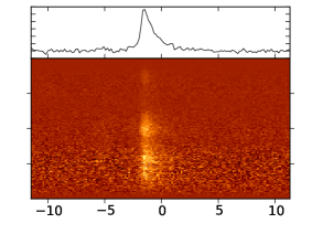
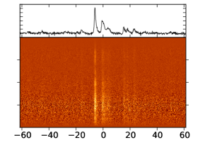
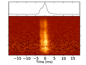
The bursts from the magnetar show a variety of temporal and spectral characteristics and phenomenology. A representative set of bursts from our 650 MHz observations are presented in Figure 4. The first two panels in each of the rows show some of the narrowest bursts and their spectral structures in the respective sessions. Most of these bursts exhibit an exponential tail, indicating scatter broadening in the intervening propagation medium. To determine the intrinsic width and scatter broadening timescale ($\tau_{\rm sc}$), we modelled the first two bursts from session S2 shown in Figure 4 as a Gaussian convolved with a one-sided exponential function (Krishnakumar et al., 2019). Our model fits suggest the intrinsic widths of the two bursts to be $0.69\pm 0.05$ ms and $0.53\pm 0.04$ ms, and the corresponding $\tau_{\rm sc}$ to be $1.30\pm 0.06$ ms and $1.05\pm 0.05$ ms, respectively. So, the apparent characteristic pulse-width of a few ms at 650 MHz is predominantly due to scatter broadening. The above intrinsic pulse-widths at 650 MHz are consistent with the characteristic pulse-width of less than 1 ms at 1360 MHz, as discussed earlier.

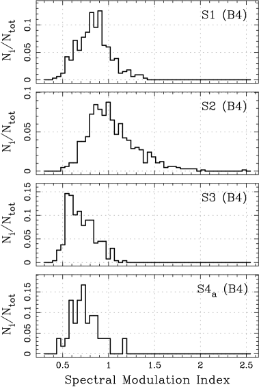
The bursts also show significant spectral variations (Figure 4). Interstellar scintillation could induce such spectral structures. However, using the above measured $\tau_{\rm sc}$, the scintillation bandwidth is estimated to be less than a kHz. Both the popular electron density models, NE2001 (Cordes & Lazio, 2002) and YMW16 (Yao et al., 2017), also suggest similar estimates. Hence, the observed spectral structures of several tens of MHz are intrinsic to the source. The structures are more prominently noticeable closer to the outburst onset (i.e., in sessions S1 and S2) and less so in the later observations. The frequency bandwidths of these structures seem to have narrowed down with time. The bursts in the later sessions appear to have more and more uniform and featureless spectra. The number of bursts which show prominent spectral variations such as those in the first row, also appear to be much lesser in the later sessions. To quantify the spectral variations, we compute spectral modulation index, $m_{I}$, defined as $m_{I}^{2}=(\overline{I^{2}}-\overline{I}^{2})/\overline{I}^{2}$, where $\overline{I}$ and $\overline{I^{2}}$ are the first and second moments of the peak-intensity of a burst as a function of frequency (Spitler et al., 2012). For each of the sessions, we selected all the bursts narrower than 3 ms and with S/N$>$10. We then computed $m_{I}$ for the dedispersed spectra corresponding to the peaks of the bursts after partially averaging in frequency to obtain 128 sub-bands across the bandwidth. The obtained $m_{I}$ are in the ranges 0.40$-$1.41, 0.49$-$2.46, 0.42$-$1.20 and 0.46$-$1.19, using 335, 660, 267 and 54 bursts from the sessions S1, S2, S3 and S4_a, respectively. The distributions of the obtained $m_{I}$ are shown in Figure 5. Note that the lowest values of $m_{I}$ in the above ranges correspond to the bursts where the spectral power is near uniformly distributed across the frequency band, and, as expected, these are indeed quite close to each other (0.40$-$0.49). A higher value of $m_{I}$ implies the spectral power to be localized in smaller sub-bands. As apparent from Figure 5, the sessions S1 and S2 have many more bursts with relatively higher $m_{I}$, and hence, with more spectral variations than the last two sessions. Moreover, in the last two sessions (S3 and S4_a), peaks of the distributions have shifted very close to the lowest observed $m_{I}$ values indicating that majority of the bursts in these sessions have close to uniform and featureless spectra.

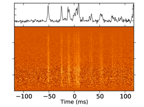
As apparent from the last panels in each of the rows in Figure 4, many times the bursts tend to occur in succession. Sometimes even a quasi-periodic occurrence is noticeable, with separations in some 5$-$25 ms range. A more quantitative characterization of the quasi-periodicity as well as the above spectral structures (e.g., measuring the structure bandwidths, and their evolution with time and frequency) will be reported elsewhere.

4 Discussion

After the previous outburst in 2003, the radio spectrum of J1810$-$197 was found to be near flat or mildly steep, with a flux density power-law index $-0.5\lesssim\alpha\lesssim 0$ (Lazaridis et al., 2008; Camilo et al., 2007). However, Dai et al. (2019) suggest the spectrum to be slightly harder after the onset of the current outburst. Their measurements on December 18 suggest $\alpha$=+0.8$\pm$0.1 in the frequency range 768$-$1800 MHz. If we include our flux density measurements below 750 MHz on the same day, we obtain $\alpha$=+1.2$\pm$0.1. This indicates that the spectrum is perhaps even harder at lower frequencies.

The period-averaged flux density has decreased rapidly since the onset of the outburst. Similar to the previous outburst (Camilo et al., 2016), the 650 MHz flux density decreased by a factor of about 5 or more in the first 20$-$30 days. The flux density at 1.52 GHz also shows a similar trend (Levin et al., 2019). Camilo et al. (2016) also showed an anti-correlation between the flux density and the spin frequency derivative during the previous outburst. However, the spin frequency derivative and 1.52 GHz flux density estimates from Levin et al. (2019, see the upper two panels in their figure 6) rather show a correlated behavior of the two parameters in the current outburst, making any possible physical link between the two further unclear.

4.1 Spiky emission: giant pulses or giant micropulses?

A working definition of giant pulses is that the flux density or pulse-energy of a single pulse averaged over the spin period is more than 10 times the corresponding mean quantity. The mean flux density of the bursts from the magnetar do not exceed the above conventional threshold. Nevertheless, the peak flux densities of the bursts are very large in absolute terms. For example, the brightest pulses in session S3 and S4 are about 2.5 and 3.5 Jy, which is 40$-$60 times the mean $S_{p}$ of the average profiles. These properties are rather reminiscent of the giant micropulses (Johnston et al., 2001) discovered from the Vela pulsar (B0833$-$45).

Much like the giant pulses, the giant micropulses add extended power-law tails to the single pulse flux density distributions (Kramer et al., 2002). The peak flux densities are often averaged over the period before making the histograms (e.g., see Karuppusamy et al., 2010). We note that the distributions of the absolute (Figure 3) as well as those of the period-averaged (not shown but analyzed separately) peak flux densities exhibit tails which are very well fit with a power-law.

Kramer et al. (2002) reported a characteristic relationship between widths of micropulses and the spin period. Using their equation 1, the expected micropulse width for J1810$-$197 would be 2.8$-$5.6 ms. While this width is consistent with the characteristic width of the bursts we measure at 650 MHz, we note that the intrinsic widths of the narrowest pulses are only about 0.5$-$0.7 ms, i.e., smaller by a factor of 4$-$5. However, the widths of the narrowest giant micropulses from the Vela pulsar are in fact also smaller than those of the average micropulses by a similar factor Kramer et al. (2002). In any case, given the scatter in the data used to derive the relationship between micropulse width and the spin period, the characteristic width of the magnetar’s bursts is consistent with the expected micropulse width. The micropulses often exhibit an associated quasi-periodicity in their occurrences. While a detailed analysis of any underlying quasi-periodicity is under progress, Figure 4 shows some examples of a possible underlying quasi-periodicity in the magnetar’s bursts.

The giant micropulses from Vela pulsar and the classical giant pulses from a handful of pulsars occur in narrow pulse phase ranges. However, the giant pulses from the Crab pulsar appear in significant parts of the pulse window. The bursts from the magnetar also do not have any favorable phase-ranges, and their occurrence rate roughly follow the integrated profile shape.

4.2 Any links with FRBs?

While most FRBs are one-off events, a couple of these are known to repeat (FRB 121102 and FRB 180814.J0422+73; Spitler et al., 2016; CHIME/FRB Collaboration et al., 2019). Recently, Hessels et al. (2019) used high time resolution observations to show complex time$-$frequency structures in the FRB 121102 bursts. Particularly, they showed that many of the bursts at 1.4 GHz show $\sim$250 MHz wide frequency bands which cannot be explained by scintillation in the ISM. Similar structures have been seen in the second repeating FRB as well (CHIME/FRB Collaboration et al., 2019). Except for the high-frequency interpulse giant-pulses from the Crab pulsar (Hankins et al., 2016) and in some faint emission components of PSR 1745$-$2900 (Pearlman et al., 2018), such frequency structures have not been seen from any known pulsar or magnetar. In Figure 4, we show that the spiky emission from J1810$-$197 also exhibits frequency structures which cannot be caused by the ISM scintillation. Hessels et al. (2019) also showed that the banded structures in many of the FRB 121102 bursts show a frequency drift, and the drift rates possibly decrease at lower frequencies. The relatively coarse time-resolution of our observations and the smearing caused by the scattering at our observing frequency does not allow adequate probes of any underlying drifts at timescales shorter than a few ms. However, the frequency drifts of FRB 180814.J0422+73 are observed at much longer timescales of some 20$-$60 ms in the frequency range 400$-$800 MHz. We do not notice such long timescale drifts in the magnetar’s bursts. In any case, high time resolution probes of the spiky emission from the magnetar at adequately high frequencies will clarify if the frequency structures indeed share some similarities with those from the repeating FRBs, for which magnetar origin is one of the popular models.

We note that the 1.36 GHz peak flux density of the brightest burst in our sample is about 9 Jy. This is about an order of magnitude larger than the peak flux density of the bright bursts from FRB 121102 at similar frequencies. However, FRB 121102 is nearly 2.8$\times$10⁵ times more distant, implying a $\sim$10¹¹ times more luminosity, for similar emission solid angles. Nevertheless, the fact that the magnetar J1810$-$197 is only the third object after the repeating FRBs and the Crab pulsar which is found to exhibit frequency structures in its bursts so prominently, might provide a phenomenological link between the underlying emission mechanisms.

5 Conclusions

To conclude, we have presented the spiky emission properties of the magnetar XTE J1810$-$197 as well as its flux density evolution and low-frequency spectrum in the early phases of the recent outburst (December 2018). We have shown that the bursts from the magnetar exhibit frequency structures that cannot be explained by interstellar scintillation. The spectral structures are easily noticeable in the early phases of the outburst, and seem to fade away in the later phases. The energetics of the spiky bursts show similarities with those of the giant micropulses, which may indicate a link between the corresponding underlying emission mechanisms. More detailed study of the spiky emission, including characterization of the frequency structures and their temporal evolution is under progress, and will be a subject of future publication.

References

- Ables et al. (1997) Ables, J. G., McConnell, D., Deshpande, A. A., & Vivekanand, M. 1997, ApJ, 475, L33
- Camilo et al. (2006) Camilo, F., Ransom, S. M., Halpern, J. P., et al. 2006, Nature, 442, 892, doi: 10.1038/nature04986
- Camilo et al. (2007) Camilo, F., Ransom, S. M., Peñalver, J., et al. 2007, ApJ, 669, 561, doi: 10.1086/521548
- Camilo et al. (2016) Camilo, F., Ransom, S. M., Halpern, J. P., et al. 2016, ApJ, 820, 110, doi: 10.3847/0004-637X/820/2/110
- CHIME/FRB Collaboration et al. (2019) CHIME/FRB Collaboration, Amiri, M., Bandura, K., et al. 2019, Nature, 566, 235, doi: 10.1038/s41586-018-0864-x
- Cordes & Lazio (2002) Cordes, J. M., & Lazio, T. J. W. 2002, ArXiv Astrophysics e-prints
- Cordes & McLaughlin (2003) Cordes, J. M., & McLaughlin, M. A. 2003, ApJ, 596, 1142
- Dai et al. (2019) Dai, S., Lower, M. E., Bailes, M., et al. 2019, ApJ, 874, L14, doi: 10.3847/2041-8213/ab0e7a
- Gotthelf et al. (2003) Gotthelf, E. V., Halpern, J. P., Markwardt, C., et al. 2003, IAU Circ., 8190
- Gupta et al. (2017) Gupta, Y., Ajithkumar, B., Kale, H. S., et al., 2017, Current Science, 113, 707-714
- Hankins et al. (2016) Hankins, T. H., Eilek, J. A., & Jones, G. 2016, ApJ, 833, 47, doi: 10.3847/1538-4357/833/1/47
- Haslam et al. (1982) Haslam, C. G. T., Salter, C. J., Stoffel, H., & Wilson, W. E. 1982, A&AS, 47, 1
- Hessels et al. (2019) Hessels, J. W. T., Spitler, L. G., Seymour, A. D., et al. 2019, ApJ, 876, L23
- Ibrahim et al. (2004) Ibrahim, A. I., Markwardt, C. B., Swank, J. H., et al. 2004, ApJL, 609, L21, doi: 10.1086/422636
- Johnston et al. (2001) Johnston, S., van Straten, W., Kramer, M., & Bailes, M. 2001, ApJ, 549, L101, doi: 10.1086/319154
- Joshi et al. (2004) Joshi, B. C., Kramer, M., Lyne, A. G., McLaughlin, M. A., & Stairs, I. H. 2004, in IAU Symposium, Vol. 218, Young Neutron Stars and Their Environments, ed. F. Camilo & B. M. Gaensler, 319
- Joshi et al. (2018) Joshi, B. C., Maan, Y., Surnis, M. P., Bagchi, M., & Manoharan, P. K. 2018, The Astronomer’s Telegram, 12312
- Karuppusamy et al. (2010) Karuppusamy, R., Stappers, B. W., & van Straten, W. 2010, A&A, 515, A36, doi: 10.1051/0004-6361/200913729
- Kramer et al. (2002) Kramer, M., Johnston, S., & van Straten, W. 2002, MNRAS, 334, 523, doi: 10.1046/j.1365-8711.2002.05478.x
- Krishnakumar et al. (2019) Krishnakumar, M. A., Maan, Y., Joshi, B. C., et al. 2019, ApJ, 878, 130
- Lazaridis et al. (2008) Lazaridis, K., Jessner, A., Kramer, M., et al. 2008, MNRAS, 390, 839, doi: 10.1111/j.1365-2966.2008.13794.x
- Levin et al. (2019) Levin, L., Lyne, A. G., Desvignes, G., et al. 2019, ArXiv e-prints. https://arxiv.org/abs/1903.02660
- Lorimer et al. (2007) Lorimer, D. R., Bailes, M., McLaughlin, M. A., Narkevic, D. J., & Crawford, F. 2007, Science, 318, 777
- Lorimer & Kramer (2004) Lorimer, D. R., & Kramer, M. 2004, Handbook of Pulsar Astronomy, ed. R. Ellis, J. Huchra, S. Kahn, G. Rieke, & P. B. Stetson
- Lyne et al. (2018) Lyne, A., Levin, L., Stappers, B., et al. 2018, The Astronomer’s Telegram, 12284
- Maan (2015) Maan, Y. 2015, ApJ, 815, 126
- Maan et al. (2012) Maan, Y., Aswathappa, H. A., & Deshpande, A. A. 2012, MNRAS, 425, 2
- Maan & Aswathappa (2014) Maan, Y., & Aswathappa, H. A. 2014, MNRAS, 445, 3221
- Margalit & Metzger (2018) Margalit, B., & Metzger, B. D. 2018, ApJ, 868, L4, doi: 10.3847/2041-8213/aaedad
- McLaughlin et al. (2006) McLaughlin, M. A., Lyne, A. G., Lorimer, D. R., et al. 2006, Nature, 439, 817
- Pearlman et al. (2018) Pearlman, A. B., Majid, W. A., Prince, T. A., et al. 2018, ApJ, 866, 160
- Ransom (2001) Ransom, S. M. 2001, PhD thesis, Harvard University
- Serylak et al. (2009) Serylak, M., Stappers, B. W., Weltevrede, P., et al. 2009, MNRAS, 394, 295, doi: 10.1111/j.1365-2966.2008.14260.x
- Spitler et al. (2012) Spitler, L. G., Cordes, J. M., Chatterjee, S., et al. 2012, ApJ, 748, 73
- Spitler et al. (2016) Spitler, L. G., Scholz, P., Hessels, J. W. T., et al. 2016, Nature, 531, 202, doi: 10.1038/nature17168
- Staelin & Reifenstein (1968) Staelin, D. H., & Reifenstein, III, E. C. 1968, Science, 162, 1481
- Surnis et al. (2016) Surnis, M. P., Joshi, B. C., Maan, Y., et al. 2016, ApJ, 826, 184, doi: 10.3847/0004-637X/826/2/184
- Thornton et al. (2013) Thornton, D., Stappers, B., Bailes, M., et al. 2013, Science, 341, 53
- Trushkin et al. (2019) Trushkin, S. A., Bursov, N. N., Tsybulev, P. G., Nizhelskij, N. A., & Erkenov, A. 2019, The Astronomer’s Telegram, 12372
- Vivekanand (2000) Vivekanand, M. 2000, ApJ, 543, 979, doi: 10.1086/317141
- Weltevrede et al. (2006) Weltevrede, P., Wright, G. A. E., Stappers, B. W., & Rankin, J. M. 2006, A&A, 458, 269, doi: 10.1051/0004-6361:20065572
- Wolszczan et al. (1984) Wolszczan, A., Cordes, J., & Stinebring, D. 1984, in Birth and Evolution of Neutron Stars: Issues Raised by Millisecond Pulsars, ed. S. P. Reynolds & D. R. Stinebring, 63
- Yao et al. (2017) Yao, J. M., Manchester, R. N., & Wang, N. 2017, ApJ, 835, 29