Spontaneous Conformal Symmetry Breaking in Fishnet CFT

Abstract

Quantum field theories with exact but spontaneously broken conformal invariance have an intriguing feature: their vacuum energy (cosmological constant) is equal to zero. Up to now, the only known ultraviolet complete theories where conformal symmetry can be spontaneously broken were associated with supersymmetry (SUSY), with the most prominent example being the $\mathcal{N}$=4 SUSY Yang-Mills. In this Letter we show that the recently proposed conformal “fishnet” theory supports at the classical level a rich set of flat directions (moduli) along which conformal symmetry is spontaneously broken. We demonstrate that, at least perturbatively, some of these vacua survive in the full quantum theory (in the planar limit, at the leading order of $1/N_{c}$ expansion) without any fine tuning. The vacuum energy is equal to zero along these flat directions, providing the first non-SUSY example of a four-dimensional quantum field theory with “natural” breaking of conformal symmetry.

Introduction

Conformal Field Theories (CFTs) represent an indispensable tool to address the behavior of many systems in the vicinity of the critical points associated with phase transitions. They also describe the limiting behavior of different quantum field theories deeply in the ultraviolet (UV) and/or infrared (IR) domains of energy. Could it be that CFTs are even more important and that the ultimate theory of Nature is conformal?

At first sight, the answer to this question is negative. Indeed, conformal invariance (CI) forbids the presence of any inherent dimensionful parameters in the action of a CFT. Because of that, CFTs have neither fundamental scales nor a well defined notion of particle states. On the other hand, Nature has both.

The loophole in these arguments is that conformal symmetry can be exact, but broken spontaneously by the ground state. This breakdown introduces an energy scale determined by the vacuum expectation value of some scalar dimensionful operator. The notion of a particle is now well defined, and in addition to massive excitations, the theory contains a massless dilaton, the Goldstone mode of the broken CI.

Theories with spontaneous breaking of conformal symmetry may be relevant for the solution of the most puzzling fine-tuning issues of fundamental particle physics, namely the hierarchy and cosmological constant problems. First, the Lagrangian of the Standard Model is invariant under the full conformal group (at the classical level) if the mass of the Higgs boson is put to zero. The observed smallness of the Fermi scale in comparison with the Planck scale might be a consequence of this Wetterich:1983bi ; Bardeen:1995kv . Second, if conformal symmetry is spontaneously broken, the energy of the ground state is equal to zero (see, e.g. Amit:1984ri ; Einhorn:1985wp ; Rabinovici:1987tf ; Shaposhnikov:2008xi and below). This fact may be relevant for the explanation of the amazing smallness of the cosmological constant.

A systematic way to construct effective field theories enjoying exact but spontaneously broken CI was described in Shaposhnikov:2008xi , following the ideas of Englert:1976ep ; Wetterich:1987fm (for further developments see Gretsch:2013ooa ; Ghilencea:2015mza ; Mooij:2018hew , for a review Wetterich:2019qzx and references therein). These theories are free from conformal anomalies but non-renormalizable. They remain in a weak coupling regime below the scale induced by the spontaneous conformal symmetry breaking. Their low energy limit may contain just the Standard Model fields, graviton plus the dilaton, which essentially decouples and does not lead to a long-range “fifth” force Wetterich:1987fm ; Shaposhnikov:2008xb ; Ferreira:2016kxi . These theories are phenomenologically viable and satisfy all possible experimental constraints. Whether they can have a well-defined UV limit remains an open question.

One can try to merge the “bottom-up” approach outlined above with the “top-down” strategy, starting from a UV complete theory. All such known CFTs are always supersymmetric. The most notable and well studied example is $\mathcal{N}=4$ SUSY Yang-Mills (SYM). Although the immediate phenomenological relevance of such theories is not clear, they are widely used as “playgrounds” for studying the spontaneous breakdown of CI.

In this Letter we show that there exists a nonsupersymmetric CFT with these properties—the recently proposed strongly $\gamma$-deformed $\mathcal{N}=4$ SYM, dubbed Conformal Fishnet Theory (FCFT)Gurdogan:2015csr  . This theory is well defined and finite at all scales and has numerous flat directions at the classical level, without fine-tuning.

Moreover, some of them, are not lifted by quantum corrections, at least in the large-$N_{c}$ limit . We will be able to demonstrate this perturbatively in the coupling constant. Among others, the reasons for these rather surprising properties for a non-SUSY theory are: i) its UV-finiteness; ii) the fact that the FCFT has a large moduli space, which increases the chances of finding directions along which CI may be broken even without resorting to unnatural tunings; iii) the supersymmetric stabilization mechanism of the parent theory is replaced by the absence of certain dangerous loop diagrams that would normally lift the classical flat directions in the Coleman-Weinberg (CW) effective potential Coleman:1973jx . This self-protection mechanism is not powerful enough to completely liberate the FCFT from all multiloop corrections on top of arbitrary flat directions, even in the planar limit. In spite of that, only a very limited sub-class of all higher loop graphs of $\phi^{4}$-type theory (in the ’t Hooft limit) is present in the effective action. All of them can be identified and their structure strongly hints towards the presence of flat vacua which are robust under quantum effects.

Before moving on, let us emphasize that there is a price to pay for these nice features: this chiral theory is not unitary. As a consequence, it is a logarithmic CFT Joao-Caetano-unpublished-2017 ; Gromov:2017cja . This is why various parameters of the broken FCFT—e.g. the induced masses and certain vertices on top of the flat vacua—are in general imaginary. Nevertheless, the FCFT can be extremely useful as it provides the so far unique possibility to test certain ideas of potential phenomenological value in the non-SUSY world.

Fishnet CFT

The FCFT involves the interacting $N_{c}\times N_{c}$ complex matrix fields $X,{\hbox to0.0pt{\hskip 2.0347pt\leavevmode\hbox{\set@color$\overline{\hbox{}}$}\hss}{\leavevmode\hbox{\set@color$X$}}},Z,{\hbox to0.0pt{\hskip 1.27083pt\leavevmode\hbox{\set@color$\overline{\hbox{}}$}\hss}{\leavevmode\hbox{\set@color$Z$}}}$ (if the theory were unitary a bar would stand for Hermitian conjugation) in the adjoint of $SU(N_{c})$; the Lagrangian at the classical level reads Gurdogan:2015csr  (see Kazakov:2018hrh for a review)

$$\mathscr{L}=N_{c}\text{tr}\left(\partial_{\mu}{\hbox to0.0pt{\hskip 2.0347pt\leavevmode\hbox{\set@color$\overline{\hbox{}}$}\hss}{\leavevmode\hbox{\set@color$X$}}}\partial_{\mu}X+\partial_{\mu}{\hbox to0.0pt{\hskip 1.27083pt\leavevmode\hbox{\set@color$\overline{\hbox{}}$}\hss}{\leavevmode\hbox{\set@color$Z$}}}\partial_{\mu}Z\\ +\tilde{\xi}^{2}{\hbox to0.0pt{\hskip 2.0347pt\leavevmode\hbox{\set@color$\overline{\hbox{}}$}\hss}{\leavevmode\hbox{\set@color$X$}}}{\hbox to0.0pt{\hskip 1.27083pt\leavevmode\hbox{\set@color$\overline{\hbox{}}$}\hss}{\leavevmode\hbox{\set@color$Z$}}}XZ\right)\ .$$ (1)

Here $\tilde{\xi}=4\pi\xi$, with the real coupling constant $\xi$ defined as $\xi^{2}=g^{2}N_{c}\,e^{-i\gamma_{3}}/(4\pi)^{2}$; $g$ is the Yang-Mills coupling constant and $\gamma_{3}$ one of the three twists of the parent $\gamma$-deformed $\mathcal{N}=4$ SYM theory . The Lagrangian (1) is obtained by considering the double-scaling limit corresponding to weak coupling and at the same time large imaginary $\gamma_{3}$, such that $\xi~{}\text{and}~{}\gamma_{1,2}~{}\text{remain finite}$.

Let us briefly review the most general properties of FCFT in the unbroken vacuum. A plethora of aspects of the theory on this conformal phase have been and are still being investigated actively; see Gurdogan:2015csr ; Gromov:2017cja ; Chicherin:2017frs ; Chicherin:2017cns ; Grabner:2017pgm ; Kazakov:2018qez ; Gromov:2018hut ; Basso:2017jwq ; Basso:2018agi ; Derkachov:2018rot ; Korchemsky:2018hnb ; Ipsen:2018fmu ; Basso:2018cvy ; Kazakov:2018gcy ; deMelloKoch:2019ywq ; Gromov:2019aku ; Gromov:2019bsj ; Chowdhury:2019hns .

A direct consequence of the strong imaginary deformation is the absence of the term corresponding to the Hermitian counterpart of the quartic interaction. This makes manifest the fact that the theory is not unitary. On the other hand, it is exactly the absence of the complex conjugate interaction term that has far reaching implications. It restricts severely the number of possible planar graphs for various physical quantities, to the point that, depending on the physical quantity, there are often none, or only a handful of diagrams, contributing at each order in the perturbative expansion.

At the same time, the fixed chirality of the interaction vertex, and the absence of the vertex of opposite chirality, forces them to possess the “fishnet” structure . This roughly means that the bulk structure of sufficiently large planar graphs is of the regular square lattice Gurdogan:2015csr . Importantly, the aforementioned chirality forbids the presence of certain diagrams, such as the ones that induce masses for the fields and the ones that renormalize the quartic coupling $\xi$. Consequently, the FCFT behaves as a fully-fledged logarithmic CFT, which implies the standard scaling properties for its local observables (i.e. correlators).

In addition, the theory appears to be integrable in the planar, ’t Hooft $N_{c}\to\infty$ limit Gurdogan:2015csr ; Caetano:2016ydc ; Gromov:2017cja , due to the integrability of the individual “fishnet” graphs discovered long ago Zamolodchikov:1980mb , see also Chicherin:2012yn  . Hence, many of the physical quantities—such as non-trivial Operator Product Expansion (OPE) data as well as certain three- and four-point correlators—are in fact exactly calculable Gromov:2018hut .

However, the model is not complete already at one-loop order: the cancellation of the divergences associated with the correlation functions of certain composite operators, such as $\text{tr}(X^{2}),\text{tr}(\hbox to0.0pt{\hskip 2.0347pt\leavevmode\hbox{\set@color$\overline{\hbox{}}$}\hss}{\leavevmode\hbox{\set@color$X$}}^{2}),\text{tr}(\hbox to0.0pt{\hskip 2.0347pt\leavevmode\hbox{\set@color$\overline{\hbox{}}$}\hss}{\leavevmode\hbox{\set@color$X$}}Z),\text{tr}(X\hbox to0.0pt{\hskip 1.27083pt\leavevmode\hbox{\set@color$\overline{\hbox{}}$}\hss}{\leavevmode\hbox{\set@color$Z$}})$, requires that in the classical action (1) new double-trace terms be included Fokken:2013aea . These read

$$\mathscr{L}_{d.t.}/(4\pi)^{2}=\alpha_{1}^{2}\left[\text{tr}(X^{2})\text{tr}(\hbox to0.0pt{\hskip 2.0347pt\leavevmode\hbox{\set@color$\overline{\hbox{}}$}\hss}{\leavevmode\hbox{\set@color$X$}}^{2})+\text{tr}(Z^{2})\text{tr}(\hbox to0.0pt{\hskip 1.27083pt\leavevmode\hbox{\set@color$\overline{\hbox{}}$}\hss}{\leavevmode\hbox{\set@color$Z$}}^{2})\right]$$ (2)

$$-\alpha_{2}^{2}\left[\text{tr}(XZ)\text{tr}(\hbox to0.0pt{\hskip 2.0347pt\leavevmode\hbox{\set@color$\overline{\hbox{}}$}\hss}{\leavevmode\hbox{\set@color$X$}}\hbox to0.0pt{\hskip 1.27083pt\leavevmode\hbox{\set@color$\overline{\hbox{}}$}\hss}{\leavevmode\hbox{\set@color$Z$}})+\text{tr}(X\hbox to0.0pt{\hskip 1.27083pt\leavevmode\hbox{\set@color$\overline{\hbox{}}$}\hss}{\leavevmode\hbox{\set@color$Z$}})\text{tr}(\hbox to0.0pt{\hskip 2.0347pt\leavevmode\hbox{\set@color$\overline{\hbox{}}$}\hss}{\leavevmode\hbox{\set@color$X$}}Z)\right] \ ,$$

with $\alpha_{1}$ and $\alpha_{2}$ couplings that, in general, depend on the renormalization scale, thus destroying, on the quantum level, the conformal symmetry. However, the beta functions for the running double-trace couplings possess two complex conjugate fixed lines, parametrized by $\xi$, with $\alpha_{1}^{2}=\pm\frac{i\xi^{2}}{2}-\frac{\xi^{4}}{2}\mp\frac{3i\xi^{6}}{4}+\mathcal{O}(\xi^{8})$ and $\alpha_{2}^{2}=\xi^{2}$, for both of them Sieg:2016vap ; Grabner:2017pgm .

The FCFT is completely defined by the explicitly local Lagrangian $\mathscr{L}+\mathscr{L}_{d.t.}$, with conformal symmetry persisting at the quantum level for the critical values of the $\alpha$’s.

Flat vacua

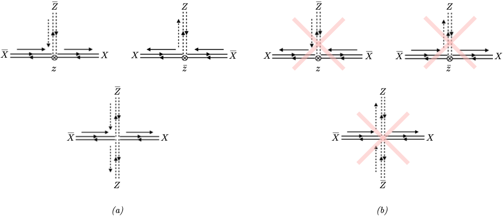
Figure 1: (a) Some of the cubic (upper graph) and the quartic (lower graph) interaction vertices that stem from the single-trace term when the Lagrangian is expanded around the symmetry-breaking vacua. A solid (dashed) line stands for the excitations $X$ or  $\overline{\hbox{}}$$X$ ($Z$ or  $\overline{\hbox{}}$$Z$), and “$\boldsymbol{\otimes}$” for the vacuum expectation value $z$ or ${\bar{z}}$. (b) The cubic (upper graph) and quartic (lower graph) vertices of opposite chirality are absent in the FCFT. To highlight this fact, we have crossed out these nonexistent vertices.

The spontaneous breaking of CI corresponds to a situation in which at least one of the fields has a non-vanishing vacuum expectation value (vev). As our CFT is non-unitary, we model this vacuum state by an extremum of the (complex) effective action.

It is important to keep in mind that once we find such a (nontrivial) saddle point, then the vacuum energy of the system automatically vanishes along this flat direction. This follows from the fact that for CFTs the potential $V$ is in general a homogeneous function of the fields $\phi_{i}$ of the theory. In other words $V\propto\phi_{i}\frac{\partial V}{\partial\phi_{i}}$, where summation over repeated indices is assumed. Provided that at least one of the fields acquires a (constant in spacetime) vev, say $\hat{\phi}_{1}\neq 0$, such that

$$\frac{\partial V}{\partial\phi_{1}}\Bigg{|}_{\hat{\phi}_{1}}=0\ ,$$ (3)

then it immediately follows that $V=0$, although mass scale(s) are now present in the theory.

Let us look for an ansatz that extremizes the potential of the FCFT. To this end, we perform the following shifts in the action

$$X\to x+X,~{}~{}~{}{\hbox to0.0pt{\hskip 2.0347pt\leavevmode\hbox{\set@color$\overline{\hbox{}}$}\hss}{\leavevmode\hbox{\set@color$X$}}}\to{\bar{x}}+\hbox to0.0pt{\hskip 2.0347pt\leavevmode\hbox{\set@color$\overline{\hbox{}}$}\hss}{\leavevmode\hbox{\set@color$X$}},~{}~{}~{}Z\to z+Z,~{}~{}~{}\hbox to0.0pt{\hskip 1.27083pt\leavevmode\hbox{\set@color$\overline{\hbox{}}$}\hss}{\leavevmode\hbox{\set@color$Z$}}\to{\bar{z}}+\hbox to0.0pt{\hskip 1.27083pt\leavevmode\hbox{\set@color$\overline{\hbox{}}$}\hss}{\leavevmode\hbox{\set@color$Z$}}\ ,$$ (4)

where $x,{\bar{x}},z,{\bar{z}}$ are the vevs of the corresponding fields, and in an abuse of notation we denoted the fluctuations again by $X,{\hbox to0.0pt{\hskip 2.0347pt\leavevmode\hbox{\set@color$\overline{\hbox{}}$}\hss}{\leavevmode\hbox{\set@color$X$}}},Z,{\hbox to0.0pt{\hskip 1.27083pt\leavevmode\hbox{\set@color$\overline{\hbox{}}$}\hss}{\leavevmode\hbox{\set@color$Z$}}}$ (as usual, these have zero vev’s).

The matrix equations of motion are obtained by varying the effective action w.r.t. $x,{\bar{x}},z,{\bar{z}}$, respectively; they read

$$-\kappa\langle\text{tr}({\hbox to0.0pt{\hskip 2.0347pt\leavevmode\hbox{\set@color$\overline{\hbox{}}$}\hss}{\leavevmode\hbox{\set@color$X$}}}^{2})\rangle x\,-\langle\text{tr}\left({\hbox to0.0pt{\hskip 2.0347pt\leavevmode\hbox{\set@color$\overline{\hbox{}}$}\hss}{\leavevmode\hbox{\set@color$X$}}}{\hbox to0.0pt{\hskip 1.27083pt\leavevmode\hbox{\set@color$\overline{\hbox{}}$}\hss}{\leavevmode\hbox{\set@color$Z$}}}\right)\rangle\,\,z-\langle\text{tr}\left({\hbox to0.0pt{\hskip 2.0347pt\leavevmode\hbox{\set@color$\overline{\hbox{}}$}\hss}{\leavevmode\hbox{\set@color$X$}}}Z\right)\rangle\,{\bar{z}}+N_{c}\,z\langle{\hbox to0.0pt{\hskip 2.0347pt\leavevmode\hbox{\set@color$\overline{\hbox{}}$}\hss}{\leavevmode\hbox{\set@color$X$}}}{\hbox to0.0pt{\hskip 1.27083pt\leavevmode\hbox{\set@color$\overline{\hbox{}}$}\hss}{\leavevmode\hbox{\set@color$Z$}}}\rangle+N_{c}\,\langle Z{\bar{x}}{\hbox to0.0pt{\hskip 1.27083pt\leavevmode\hbox{\set@color$\overline{\hbox{}}$}\hss}{\leavevmode\hbox{\set@color$Z$}}}\rangle+N_{c}\,\langle Z{\hbox to0.0pt{\hskip 2.0347pt\leavevmode\hbox{\set@color$\overline{\hbox{}}$}\hss}{\leavevmode\hbox{\set@color$X$}}}\rangle{\bar{z}}+N_{c}\,\langle Z{\hbox to0.0pt{\hskip 2.0347pt\leavevmode\hbox{\set@color$\overline{\hbox{}}$}\hss}{\leavevmode\hbox{\set@color$X$}}}{\hbox to0.0pt{\hskip 1.27083pt\leavevmode\hbox{\set@color$\overline{\hbox{}}$}\hss}{\leavevmode\hbox{\set@color$Z$}}}\rangle=$$ (5)

$$=\text{tr}({\bar{x}}^{2})x+\text{tr}\left({\bar{x}}{\bar{z}}\right)z+\text{tr}\left({\bar{x}}z\right)\,{\bar{z}}-N_{c}\,z{\bar{x}}{\bar{z}}\ ,$$

$$-\kappa\langle\text{tr}(X^{2})\rangle{\bar{x}}\,-\langle\text{tr}\left(X{\hbox to0.0pt{\hskip 1.27083pt\leavevmode\hbox{\set@color$\overline{\hbox{}}$}\hss}{\leavevmode\hbox{\set@color$Z$}}}\right)\rangle\,\,z-\langle\text{tr}\left(XZ\right)\rangle\,{\bar{z}}+N_{c}\,\langle{\hbox to0.0pt{\hskip 1.27083pt\leavevmode\hbox{\set@color$\overline{\hbox{}}$}\hss}{\leavevmode\hbox{\set@color$Z$}}}XZ\rangle+N_{c}\,{\bar{z}}\langle XZ\rangle+N_{c}\,\langle{\hbox to0.0pt{\hskip 1.27083pt\leavevmode\hbox{\set@color$\overline{\hbox{}}$}\hss}{\leavevmode\hbox{\set@color$Z$}}}xZ\rangle+N_{c}\,\langle{\hbox to0.0pt{\hskip 1.27083pt\leavevmode\hbox{\set@color$\overline{\hbox{}}$}\hss}{\leavevmode\hbox{\set@color$Z$}}}X\rangle z=$$ (6)

$$=\text{tr}(x^{2}){\bar{x}}+\text{tr}\left(x{\bar{z}}\right)z+\text{tr}\left(xz\right)\,{\bar{z}}-N_{c}\,{\bar{z}}xz\ ,$$

$$-\langle\text{tr}({\hbox to0.0pt{\hskip 2.0347pt\leavevmode\hbox{\set@color$\overline{\hbox{}}$}\hss}{\leavevmode\hbox{\set@color$X$}}}{\hbox to0.0pt{\hskip 1.27083pt\leavevmode\hbox{\set@color$\overline{\hbox{}}$}\hss}{\leavevmode\hbox{\set@color$Z$}}})\rangle x\,-\langle\text{tr}\left(X{\hbox to0.0pt{\hskip 1.27083pt\leavevmode\hbox{\set@color$\overline{\hbox{}}$}\hss}{\leavevmode\hbox{\set@color$Z$}}}\right)\rangle\,{\bar{x}}-\kappa\langle\text{tr}\left({\hbox to0.0pt{\hskip 1.27083pt\leavevmode\hbox{\set@color$\overline{\hbox{}}$}\hss}{\leavevmode\hbox{\set@color$Z$}}}^{2}\right)\rangle\,z+N_{c}\,{\bar{x}}\langle{\hbox to0.0pt{\hskip 1.27083pt\leavevmode\hbox{\set@color$\overline{\hbox{}}$}\hss}{\leavevmode\hbox{\set@color$Z$}}}X\rangle+N_{c}\,\langle{\hbox to0.0pt{\hskip 2.0347pt\leavevmode\hbox{\set@color$\overline{\hbox{}}$}\hss}{\leavevmode\hbox{\set@color$X$}}}{\bar{z}}X\rangle+N_{c}\,\langle{\hbox to0.0pt{\hskip 2.0347pt\leavevmode\hbox{\set@color$\overline{\hbox{}}$}\hss}{\leavevmode\hbox{\set@color$X$}}}{\hbox to0.0pt{\hskip 1.27083pt\leavevmode\hbox{\set@color$\overline{\hbox{}}$}\hss}{\leavevmode\hbox{\set@color$Z$}}}\rangle x+N_{c}\,\langle{\hbox to0.0pt{\hskip 2.0347pt\leavevmode\hbox{\set@color$\overline{\hbox{}}$}\hss}{\leavevmode\hbox{\set@color$X$}}}{\hbox to0.0pt{\hskip 1.27083pt\leavevmode\hbox{\set@color$\overline{\hbox{}}$}\hss}{\leavevmode\hbox{\set@color$Z$}}}X\rangle=$$ (7)

$$=\text{tr}({\bar{x}}{\bar{z}})x+\text{tr}\left(x{\bar{z}}\right){\bar{x}}+\kappa\text{tr}\left({\bar{z}}^{2}\right)\,z-N_{c}\,{\bar{x}}{\bar{z}}x\ ,$$

$$-\langle\text{tr}({\hbox to0.0pt{\hskip 2.0347pt\leavevmode\hbox{\set@color$\overline{\hbox{}}$}\hss}{\leavevmode\hbox{\set@color$X$}}}Z)\rangle x\,-\langle\text{tr}\left(XZ\right)\rangle\,{\bar{x}}-\kappa\langle\text{tr}\left(Z^{2}\right)\rangle\,{\bar{z}}+N_{c}\,x\langle Z{\hbox to0.0pt{\hskip 2.0347pt\leavevmode\hbox{\set@color$\overline{\hbox{}}$}\hss}{\leavevmode\hbox{\set@color$X$}}}\rangle+N_{c}\,\langle Xz{\hbox to0.0pt{\hskip 2.0347pt\leavevmode\hbox{\set@color$\overline{\hbox{}}$}\hss}{\leavevmode\hbox{\set@color$X$}}}\rangle+N_{c}\,\langle XZ\rangle{\bar{x}}+N_{c}\,\langle XZ{\hbox to0.0pt{\hskip 2.0347pt\leavevmode\hbox{\set@color$\overline{\hbox{}}$}\hss}{\leavevmode\hbox{\set@color$X$}}}\rangle=$$ (8)

$$=\text{tr}({\bar{x}}z)x+\text{tr}\left(xz\right){\bar{x}}+\kappa\text{tr}\left(z^{2}\right)\,{\bar{z}}-N_{c}\,xz{\bar{x}}\ .$$

Here $\kappa=-2\alpha^{2}_{1}/\xi^{2}$, $\langle\dots\rangle$ denotes the quantum average of the corresponding quantity w.r.t. the action with the shifted fields (4), and we took into account the planar limit.

Notice that the presence of the non-Hermitian single-trace interaction term, as well as the fact that $\kappa$ is complex at the conformal point, results into the equations for the fields and their would-be Hermitian counterparts to not be related by complex conjugation. In turn, the solutions to the above equations for the pairs $x,{\bar{x}}$ and $z,{\bar{z}}$ need not necessarily be complex conjugates, so the vev’s may be viewed as four independent constants in the space of matrix fields. We will see that this may have important consequences for the quantum fate of the flat directions.

Classical flat vacua

Turning to the existence of (nontrivial) vacua, we note that classically, i.e. in the tree approximation, all the deviations $X,{\hbox to0.0pt{\hskip 2.0347pt\leavevmode\hbox{\set@color$\overline{\hbox{}}$}\hss}{\leavevmode\hbox{\set@color$X$}}},Z,{\hbox to0.0pt{\hskip 1.27083pt\leavevmode\hbox{\set@color$\overline{\hbox{}}$}\hss}{\leavevmode\hbox{\set@color$Z$}}}$ of the fields in (LABEL:eq:gen_eq1)-(LABEL:eq:gen_eq4) should be put to zero (and there is no quantum average). Thus, the classical flatness conditions are reduced to the r.h.s. of these equations being zero.

For simplicity, we will work with configurations for which $x_{\rm tree}={\bar{x}}_{\rm tree}=0$ , such that the first two of the equations of motion are identically satisfied, while the last two become (since $\kappa\neq 0$)

$$\text{tr}\left({\bar{z}}_{\rm tree}^{2}\right)z_{\rm tree}=0\ ,~{}~{}~{}\text{and}~{}~{}~{}\text{tr}\left(z_{\rm tree}^{2}\right){\bar{z}}_{\rm tree}=0\ ,$$ (9)

with $z_{\rm tree}$ and ${\bar{z}}_{\rm tree}$ (constant) classical fields subject to

$$\text{tr}\left(z_{\rm tree}\right)=\text{tr}\left({\bar{z}}_{\rm tree}\right)=0\ ,$$ (10)

due to the unimodularity of the global $SU(N_{c})$ symmetry. Inspection of (9) reveals that, at least at the classical level, the fishnet CFT has a plethora of nontrivial symmetry breaking solutions, at any value of the coupling $\xi$ . Interestingly, some are not present in the full $\mathcal{N}=4$ SYM nor in its $\gamma$–deformed descendant; rather, they emerge when the strong imaginary $\gamma$-deformation limit—leading to the fishnet CFT—is considered. A complete classification of the moduli space of the FCFT, however, lies well beyond the scope of the present paper. Therefore, here we will focus on the simplest possible symmetry breaking flat vacua that we have been able to find and leave the search and study for more complicated ones for the future.

The first option is to take $z_{\rm tree}$ and ${\bar{z}}_{\rm tree}$ to be nonzero, related by complex conjugation, and diagonal , i.e.

$$z_{\rm tree}=v\,\text{diag}\left(z_{1},\ldots,z_{N_{c}}\right)\ ,$$ (11)

$${\bar{z}}_{\rm tree}=\bar{v}\,\text{diag}\left({\bar{z}}_{1},\ldots,{\bar{z}}_{N_{c}}\right)\ ,$$

with $v$ a (complex) parameter with dimension of mass and $z_{k}$ are, in general, complex numbers . Since by construction $z_{\rm tree}\neq 0$ (and consequently ${\bar{z}}_{\rm tree}\neq 0$), the only option for both equations to hold is to require that

$$\sum_{k=1}^{N_{c}}z_{k}^{2}=\sum_{k=1}^{N_{c}}\bar{z}_{k}^{2}=0\ .$$ (12)

The second class of symmetry breaking solutions to eqs. (LABEL:eq:gen_eq1)-(LABEL:eq:gen_eq4) comprises vacua for which the fields $X$ and  $\overline{\hbox{}}$$X$, and $Z$ and  $\overline{\hbox{}}$$Z$, are not related by complex conjugation. As we have already pointed out, this is certainly a possibility, due to the non-Hermiticity of the theory. We may therefore assume that $z_{\rm tree},{\bar{z}}_{\rm tree}\neq 0$ and subject to (9) and (10). As we will show in the next section, such configurations may be rather interesting when it comes to quantum corrections.

Yet another acceptable choice is to put $x_{\rm tree}={\bar{x}}_{\rm tree}={\bar{z}}_{\rm tree}=0$, while $z_{\rm tree}$ can be an arbitrary traceless $N_{c}\times N_{c}$ matrix. Interestingly, even though conformal symmetry is broken spontaneously along such flat directions, the spectrum of the theory contains only massless degrees of freedom, at least in the planar limit.

The third and final category of “natural” flat directions we will be reporting on here involves nilpotent matrices of index 2, i.e. $z_{\rm tree}\neq 0$, while $z_{\rm tree}^{2}=0$. Interestingly, such vacua appear also in beyond the Standard Model phenomenology, see Maiezza:2016ybz . Like in the previous case—and unlike what happens with Hermitian theories—all the excitations on top of these vacua in the leading $N_{c}$ order are massless, in spite of the fact that conformal symmetry is clearly broken. More details on the spectrum of excitations around the aforementioned classes of vacua can be found in the Appendix A.

Before moving on, let us stress that the existence of flat directions for arbitrary $\xi$—even at the classical level—is a rather salient point that deserves some discussion. One might expect that whether or not the theory possesses ground states with nonlinearly realized conformal symmetry would crucially depend on the specific value of the coupling constant. This is precisely what happens in other nonsupersymmetric CFTs such as the massless $\phi^{4}$ theory and its generalizations Shaposhnikov:2008xb , where finetunings are required in order for CI to be spontaneously broken down to Poincaré Fubini:1976jm , see also Coradeschi:2013gda . On the contrary, the FCFT has many vacua (some of which are inherited from its parent $\mathcal{N}=4$ SYM) with vanishing energy, without the need for finetuning. Equivalently, the dilaton—that is part of the theory’s spectrum in the Coulomb phase—has zero mass, naturally.

In the following we will argue that this phenomenon persists at the quantum level and in the planar limit, at least for some of the vacua we found.

Quantum Coleman-Weinberg effective potential

To study the fate of conformal symmetry breaking at the quantum level, we will also confine ourselves to “$z$-vacua,” for which $x={\bar{x}}=0$. It is important to keep in mind that, with such an ansatz, the extrema of the effective action do not break the discrete symmetry $X\to-X,\,{\hbox to0.0pt{\hskip 2.0347pt\leavevmode\hbox{\set@color$\overline{\hbox{}}$}\hss}{\leavevmode\hbox{\set@color$X$}}}\to-{\hbox to0.0pt{\hskip 2.0347pt\leavevmode\hbox{\set@color$\overline{\hbox{}}$}\hss}{\leavevmode\hbox{\set@color$X$}}}$, meaning that we can drop all terms containing averages with odd powers of these two fields from (LABEL:eq:gen_eq1)-(LABEL:eq:gen_eq4).

Consequently, only the last two of these equations survive and boil down to 

$$\tfrac{\kappa}{N_{c}}\text{tr}\left({\bar{z}}^{2}\right)z=\left\langle{\hbox to0.0pt{\hskip 2.0347pt\leavevmode\hbox{\set@color$\overline{\hbox{}}$}\hss}{\leavevmode\hbox{\set@color$X$}}}{\bar{z}}X\right\rangle-\tfrac{\kappa}{N_{c}}\left\langle\text{tr}({\hbox to0.0pt{\hskip 1.27083pt\leavevmode\hbox{\set@color$\overline{\hbox{}}$}\hss}{\leavevmode\hbox{\set@color$Z$}}}^{2})\right\rangle z+\left\langle{\hbox to0.0pt{\hskip 2.0347pt\leavevmode\hbox{\set@color$\overline{\hbox{}}$}\hss}{\leavevmode\hbox{\set@color$X$}}}{\hbox to0.0pt{\hskip 1.27083pt\leavevmode\hbox{\set@color$\overline{\hbox{}}$}\hss}{\leavevmode\hbox{\set@color$Z$}}}X\right\rangle,$$ (13)

$$\tfrac{\kappa}{N_{c}}\text{tr}\left(z^{2}\right){\bar{z}}=\left\langle Xz{\hbox to0.0pt{\hskip 2.0347pt\leavevmode\hbox{\set@color$\overline{\hbox{}}$}\hss}{\leavevmode\hbox{\set@color$X$}}}\right\rangle-\tfrac{\kappa}{N_{c}}\left\langle\text{tr}(Z^{2})\right\rangle{\bar{z}}+\left\langle XZ{\hbox to0.0pt{\hskip 2.0347pt\leavevmode\hbox{\set@color$\overline{\hbox{}}$}\hss}{\leavevmode\hbox{\set@color$X$}}}\right\rangle.$$

The one-loop effective potential

Whether or not quantum corrections jeopardize the CI by uplifting the flat directions can be demonstrated already at the first loop order, by investigating the CW effective potential Coleman:1973jx .

In this approximation $\alpha_{1}^{2}=\pm i\xi^{2}/2$, so we can set $\kappa=\pm i$. In addition, the last terms in (LABEL:1loop_tadpoles) are irrelevant (they correspond to higher order Feynman graphs). In the planar limit, the second and third terms are given by the diagrams presented in Fig. 2.

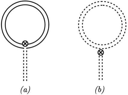
Figure 2: The one-loop tadpole diagrams stemming from the single- and double- trace terms—$(a)$ and $(b)$, respectively. A solid (dashed) line stands for the excitations $X$ or  $\overline{\hbox{}}$$X$ ($Z$ or  $\overline{\hbox{}}$$Z$), and “$\boldsymbol{\otimes}$” for the vacuum expectation value $z$ or ${\bar{z}}$. We have suppressed the color and chirality arrows.

As we did in the classical considerations, let us require that $z$ and ${\bar{z}}$ be diagonal matrices. The evaluation of the one-loop tadpole diagrams is straightforward in this case, see Appendix B. The matrix equations (LABEL:1loop_tadpoles) take the explicit form

$$\pm i\text{tr}\left({\bar{z}}^{2}\right)=\xi^{2}\left[\text{tr}({\bar{z}}^{2})\log\frac{z}{\sqrt{Q}}+\text{tr}\left({\bar{z}}^{2}\log\frac{{\bar{z}}}{\sqrt{Q}}\right)\right],$$

$$\pm i\text{tr}\left(z^{2}\right)=\xi^{2}\left[\text{tr}(z^{2})\log\frac{{\bar{z}}}{\sqrt{Q}}+\text{tr}\left(z^{2}\log\frac{z}{\sqrt{Q}}\right)\right],$$

with $Q=\sqrt{{\rm tr}(z^{2})\,{\rm tr}({\bar{z}}^{2})}$; note that due to the non-Hermiticity of the FCFT the sign in the l.h.s. of both equations must be the same—either plus or minus. The absence of sources breaking explicitly the CI of the theory translates into the effective potential (and its derivatives) to exhibit no dependence on the ’t Hooft-Veltman renormalization scale $\mu$. In turn, the derivatives of the potential w.r.t. the fields are related to the beta function of $\xi$, which vanishes by construction. Let us stress that at large $N_{c}$, none of the physical quantities—such as correlators of local fields—can actually depend on $\mu$ for the chosen background fields $z,{\bar{z}}$, since in the UV regime the theory behaves like in the unbroken phase, which is UV finite. The CW potential is yet another example of such a quantity.

We notice immediately that it is in principle possible to put to zero the tree-level and one-loop parts of the potential separately, provided that the vacuum (LABEL:eq:Zvev), apart from the constraints (10) and (12), is also subject to

$$\sum_{k=1}^{N_{c}}z_{k}^{2}\log z_{k}=\sum_{k=1}^{N_{c}}\bar{z}_{k}^{2}\log\bar{z}_{k}=0\ .$$ (15)

This condition picks up a particular subclass of the classical vacua discussed in the previous section. At the one-loop order these are not lifted by quantum effects. As a result, the vacuum energy of the loop corrected theory on top of these flat directions is zero, or in other words, the masslessness of the dilaton persists at one-loop level. It should be stressed that this is a unique situation for a non-SUSY four-dimensional theory.

Let us give a simple example of a flat vacuum which is robust under one loop quantum corrections. Take $x={\bar{x}}=0$ and $z$ to be a block-diagonal matrix comprising $N_{c}/4$ diagonal sub-blocks each with dimensions $4\times 4$

$$z=v\,\text{diag}(\underbrace{z_{1},z_{2},z_{3},z_{4}},\underbrace{z_{1},z_{2},z_{3},z_{4}},\ldots)\ ,$$ (16)

and ${\bar{z}}$ is its Hermitian conjugate in this case. Plugging (16) into the system of transcendental eqs. (10), (12) and (15), we numerically find a complex (as a consequence of the non-unitarity) solution

$$z_{1} =-0.587849-0.808971\,i\,,~{}z_{2}=0.260305+1.45187\,i\,,$$ (17)

$$z_{3} =1.32754-0.642903\,i\,,~{}~{}~{}~{}\,\,z_{4}=-1\,,$$

where the overall rescaling $z_{j}\to{\rm const}\times z_{j}$ was absorbed into the complex modulus $v$ labeling the one-parameter family of flat vacua .

There is no difficulty in finding more examples for larger block matrices of the form (16), and thus with more of the parameters labeling the flat vacua. For instance if we solve the system of eqs. (10), (12) and (15) for $z$ made of $N_{c}/5$ sub-blocks of dimensions $5\times 5$, we will have an extra parameter, in addition to $v$, parametrizing the flat directions. We can also mix sub-blocks of different sizes.

Although this is certainly an interesting option, as we will now demonstrate, it is not the only one. Actually, it is possible to arrange a situation in which the tree-level and one-loop contributions are of the same order of magnitude and can in principle balance each other out. Remarkably, this enables the perturbative analysis of the flat vacua and is in close analogy to what happens in the CW effective potential in gauge theories Coleman:1973jx . In the present context, we can achieve this by keeping the order of magnitude of the vacuum fields $z_{k},{\bar{z}}_{k}\sim 1$, while ${\rm tr}(z^{2})\sim{\rm tr}({\bar{z}}^{2})\sim N_{c}\,{\cal O}(\xi^{2})$. To this end, let us stick to vacua comprising diagonal matrices, assume that $z={\bar{z}}=v\,\text{diag}(z_{1},\ldots,z_{N_{c}})$, but relax the requirement (12). For instance, we may consider the following perturbative vacuum

$$z_{k}=z_{k}^{(0)}+\varepsilon(\xi)z_{k}^{(1)}+\eta(\xi)z_{k}^{(2)}+\ldots\ ,$$ (18)

with $z_{k}^{(i)}$’s complex and subject to $\sum_{k}z_{k}^{(i)}=0~{}\forall~{}i$, in order for the unimodularity constraint (10) to be satisfied. In the above, $\varepsilon(\xi)\sim c_{1}^{\varepsilon}\xi^{2}+c_{2}^{\varepsilon}\xi^{4}+\ldots,\eta(\xi)\sim c_{1}^{\eta}\xi^{2}+\ldots$ admit perturbative expansions in terms of the coupling and can be determined iteratively at each order by plugging $z_{k}$ into (The one-loop effective potential) and requiring that the equations be satisfied. As a proof of concept, let us pick the following specific, but by no means unique, one-loop vacuum

$$z_{k}={\bar{z}}_{k}=e^{2\pi i(k-1)/N_{c}}+c_{1}^{\varepsilon}\xi^{2}\,e^{-2\pi i(k-1)/N_{c}}\ ,$$ (19)

such that $\sum_{k}z_{k}^{2}=2c_{1}^{\varepsilon}\xi^{2}\,N_{c}\neq 0$ and $\sum_{k}z_{k}^{2}\log z_{k}\approx N_{c}/2$. At order $\xi^{2}$, only the terms proportional to ${\rm tr}(z^{2}\log z)$ and ${\rm tr}({\bar{z}}^{2}\log{\bar{z}})$ contribute from the right-hand side of the equations (The one-loop effective potential). It is straightforward to see that $c_{1}^{\varepsilon}=\pm i/4$, meaning that, up to a factor of $1/2$, $\varepsilon(\xi)$ coincides with $\alpha_{1}^{2}$ at one loop order, i.e. an acceptable one-loop flat direction is

$$z_{k}=e^{2\pi i(k-1)/N_{c}}+\frac{\alpha_{1}^{2}}{2}\,e^{-2\pi i(k-1)/N_{c}}\ .$$ (20)

Before we move to the discussion of multiloop contributions to the CW potential, let us note en passant, that for massless excitations, the one-loop contributions to the effective potential vanish identically. This means that vacua for which the fields are either not related by complex conjugation and only one of $z$, ${\bar{z}}$ is nonvanishing, or are nilpotent matrices, do not receive any corrections at the one-loop level. Actually, this holds true at all orders of perturbation theory as we will see in a while. This is due to the chirality of the theory that allows for specific types of vertices only, as well as the masslessness of the particles running in the loops. Of course, such flat directions are in a sense quite peculiar, as the CI is spontaneously broken but the spectrum of the theory does not accommodate any massive particles, in the large-$N_{c}$ limit.

Higher-loop corrections to the effective potential

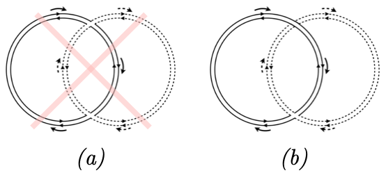
Figure 3: $(a)$ The chirality of the theory forbids some of the diagrams that would contribute to the effective potential at higher orders, such as the one above appearing in $\mathcal{O}(\xi^{4})$. $(b)$ Example of a possible non-planar vacuum diagram in the leading $\xi^{2}$ order, to be neglected in the ’t Hooft limit.

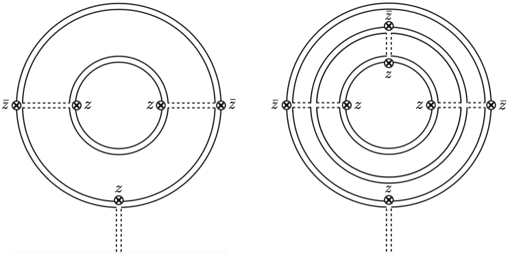
Figure 4: Exemplary multiloop tadpole diagrams of the fishnet type stemming from the single trace term. The specific three loop diagram (left) contains only cubic vertices, while the six loop one (right) contains both cubic as well as quartic vertices. The chirality of the theory forces the higher order planar diagrams stemming from the single-trace term to be of this form.

Let us now proceed to the possible multiloop corrections to the effective potential and study under which conditions and/or modifications our considerations persist.

Let us focus first on the contributions from the single trace term of the potential, $\text{tr}(\hbox to0.0pt{\hskip 2.0347pt\leavevmode\hbox{\set@color$\overline{\hbox{}}$}\hss}{\leavevmode\hbox{\set@color$X$}}\hbox to0.0pt{\hskip 1.27083pt\leavevmode\hbox{\set@color$\overline{\hbox{}}$}\hss}{\leavevmode\hbox{\set@color$Z$}}XZ)$. When the Lagrangian is expanded around the symmetry-breaking vacua, see Appendix A, the cubic and quartic terms give rise to the “chiral” vertices presented in Fig. 1(a). In essence, we may view the trivalent vertices of the theory as the quartic chiral vertex with one of the legs removed and replaced by the corresponding expectation value, but otherwise preserving its double-line structure and chirality. Their presence leads to planar graphs similar to the ones built exclusively with a chiral quartic vertex, but with some propagators, or parts of the closed loops of $X$ (or $Z$) propagators removed (we call them loops with amputated propagators). It is important to keep in mind that the non-Hermiticity of the FCFT translates into a fixed chirality of the vertices. In other words, the absence of the complex conjugate counterpart of $\text{tr}(\hbox to0.0pt{\hskip 2.0347pt\leavevmode\hbox{\set@color$\overline{\hbox{}}$}\hss}{\leavevmode\hbox{\set@color$X$}}\hbox to0.0pt{\hskip 1.27083pt\leavevmode\hbox{\set@color$\overline{\hbox{}}$}\hss}{\leavevmode\hbox{\set@color$Z$}}XZ)$ is in one-to-one with the absence of the “anti-chiral” vertices presented in Fig. 1(b) and marked with red.

It is now straightforward to see that without the anti-chiral vertices, the “zoo” of possible Feynman diagrams is rather restricted. For example, the diagram Fig. 3$(a)$ with two quartic vertices is absent from FCFT, even on top of vacua breaking conformal symmetry, due to the opposite chirality of the single-trace vertices there. Note that many more kinds of graphs exist, like the one given in Fig. 3$(b)$, with one quartic vertex but with higher than spherical topology. They will certainly modify the CW potential in the $1/N^{2}_{c}$ order of the ’t Hooft expansion, which we don’t consider here. Of course this simplifies considerably the situation. Nevertheless, the effective potential at higher orders may receive contributions—among others—from fishnet diagrams (with possibly amputated propagators, as explained above). Two graphs of this type are presented in Fig. 4. Their types, and hence their number, are very limited w.r.t. the generic graphs of scalar QFT at each order in perturbation theory; unfortunately, they are still too complicated for explicit computations . For our purposes, however, it suffices to understand what happens qualitatively. In the $z$-vacua under consideration, such graphs can be only made of nested concentric circles of $X$-propagators connected by ”radial” $Z$-propagators (possibly crossing the circles via quartic vertices) that end up on cubic vertices. Note that the $X$ propagator (and the off-diagonal parts of the $Z$ propagator) can connect cubic vertices of the same type only, in contrast to the diagonal components of the $Z$ propagator that necessarily connect different vertices.

As for the diagrams following from the double-trace terms, they can only contribute to the large-$N_{c}$ limit if they occur in the graphs in such a way that they connect two, otherwise disconnected, parts of the graph (corresponding to each of two traces from the double-trace vertex) Gromov:2018hut ; Fokken:2014soa . An example of such graph is drawn in Fig. 5. Like in the one-loop considerations, the contributions coming from the double-trace terms must exactly cancel the $\mu$-dependence from the single-trace terms, as required by the conformality of the FCFT.

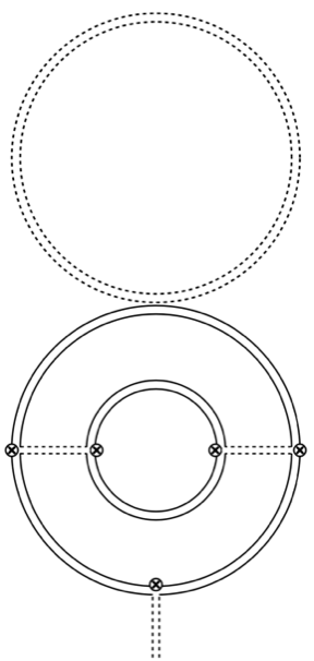
Figure 5: Typical planar graph that feeds into the (derivatives of the) effective potential at four loops.

Several important comments are in order here. First of all, for the “exotic” vacua in which ${\bar{z}}=0$ and $z\neq 0$ or vice-versa, the tree-level potential is exact. In other words, it receives no loop corrections, at any order in perturbation theory. This is either because the diagrams cannot be constructed to start with, or they vanish identically (in dimensional regularization) since the particles running in the loops are massless.

The same is also true for the nilpotent vacua. Although both types of vertices may be present (assuming that the fields are related by complex conjugation), the corresponding diagrams vanish automatically, either because they are proportional to traces of $z^{p}=0$, for $p\geq 2$ (one always finds such traces for the innermost circle of Fig. 4), or because, again, the excitations are massless.

One cannot conclude the same for the more interesting symmetry breaking solutions of the previous section, when both $z,{\bar{z}}$ are diagonal. Then the higher order diagrams in the effective potential, such as of the type presented on Fig. 4, do not vanish. To see this more clearly, let us focus on the three loop graph on the left of this figure. On top of the diagonal vacuum (LABEL:eq:Zvev), it is equal to

$$\bar{v}v^{2}\left(\tilde{\xi}^{2}\right)^{4}\sum_{k,l,m}\bar{z}_{k}^{2}z_{l}^{3}\int\frac{d^{4}p_{1}\,d^{4}p_{2}\,d^{4}p_{3}/(4\pi)^{3}}{p_{1}^{4}(p_{2}^{2}+{\bar{z}}_{k}z_{j})((p_{1}+p_{2})^{2}+z_{k}z_{m})}\times$$

$$~{}~{}~{}~{}~{}~{}~{}~{}~{}~{}~{}~{}~{}~{}~{}~{}~{}~{}\times\frac{1}{(p_{3}^{2}+{\bar{z}}_{m}z_{l})((p_{1}+p_{3})^{2}+{\bar{z}}_{j}z_{l})^{2}}\ ,$$

where $p_{i}$’s are dimensionless. This integral has logarithmic UV divergences but once we add to it all diagrams of the same loop order (containing double-trace vertices as well) it is guaranteed by conformal symmetry that, as in the one-loop case, the overall result will be nonzero, finite and scheme independent. Actually, it would be interesting to explicitly compute it, a difficult but not impossible problem, which however lies beyond our purposes here.

On general dimensional grounds, we expect loop corrections to the effective potential to be of the following form

$$V_{n-loop}=c_{n}\left(\tilde{\xi}^{2}\right)^{n+1}\text{tr}(z^{2})\,\text{tr}({\bar{z}}^{2})f^{(n)}[z,\bar{z}]\ ,$$ (21)

where $c_{n}$ are numerical factors, and $f^{(n)}[z,\bar{z}]$ homogeneous functions of degree zero w.r.t. $z$ and ${\bar{z}}$, symmetric w.r.t. the permutations of pairs of eigenvalues $(z_{j},{\bar{z}}_{j})\to(z_{k},{\bar{z}}_{k})$. For instance, at the one loop level

$$f^{(1)}=\frac{\text{tr}\left(z^{2}\log\frac{z}{\sqrt{Q}}\right)}{\text{tr}(z^{2})}+\frac{\text{tr}\left(\bar{z}^{2}\log\frac{\bar{z}}{\sqrt{Q}}\right)}{\text{tr}(\bar{z}^{2})}\ ,$$ (22)

while at two loops, schematically

$$f^{(2)} \propto f^{(1)}+c\left(\frac{\text{tr}\left(z^{2}\log^{2}\frac{z}{\sqrt{Q}}\right)}{\text{tr}(z^{2})}+\frac{\text{tr}\left(\bar{z}^{2}\log^{2}\frac{\bar{z}}{\sqrt{Q}}\right)}{\text{tr}(\bar{z}^{2})}\right)\ .$$

Like we did in the one-loop approximation, we have a number of options. The first is to require that the higher-loop contributions vanish independently from the ones coming from the lowest orders. This would mean that in addition to (12) and (15), we have to further restrict the flat directions, since we will encounter new patterns of traces in higher loops. For example, for the 2-loop correction we will have to impose $\text{tr}\left(z^{2}\log^{2}z\right)=0$ as well. To fulfill simultaneously all the flatness constraints, will certainly take larger than the 4$\times$4 sub-matrices we worked with previously. This is a procedure that has to be effectuated repeatedly, and it is conceivable that more than one conditions may be required at each loop order.

Alternatively, we may insist that the tree level and one-loop contributions vanish independently from each other by virtue of (12) and (15), while the higher loop corrections are taken care of by “perturbing” this solution in the sense of (18). This way, all quantum corrections starting from a specific loop order will be comparable by design so they may compensate for each other.

Finally, we can stick with the perturbative vacua (18) and appropriately generalize them by keeping higher powers of $\xi$ and even use different harmonics so that all the terms in the effective potential will be of the same order. By doing so, we need only to impose one condition per loop order: that is, the derivative(s) of the full effective potential w.r.t. the fields be zero. This option is attractive since, in principle, we have the possibility to study it perturbatively, order by order.

Conclusions and open problems

In this work we initiated the study of spontaneous conformal symmetry breaking in the recently proposed fishnet CFT. We showed that the theory admits a plethora of classical flat directions along which conformal symmetry is nonlinearly realized without fine-tuning. We also studied the quantum corrections and found that the classical conformal invariance is not violated, at least in some subclasses of the classical solutions. This fact is the (nontrivial) aftermath of a delicate interplay between the finiteness of the theory, its non-Hermiticity, the large-$N_{c}$ limit and the constraints on the flat directions.

The FCFT is integrable in ’t Hooft limit. Although the integrability is demonstrated only for the unbroken vacuum, some features of it may survive for the broken vacua, at least in perturbation theory. This could offer a unique opportunity to elucidate various aspects of the dynamics behind spontaneous symmetry breaking in this particular theory. At the same time, it can serve as an inspiring example for CFTs with such behavior in general. A first step towards this direction could be to check the validity of the constraints that were derived in Karananas:2017zrg . For instance, the deep infrared limit of the two-point functions of scalar primary operators $\mathcal{O}_{I}$ were shown to obey the identity

$$\langle\mathcal{O}_{I}\rangle\langle\mathcal{O}_{J}\rangle\sim\lim_{x\to\infty}\sum_{K}\frac{c_{IJK}}{|x|^{\Delta_{I}+\Delta_{J}-\Delta_{K}}}\langle\mathcal{O}_{K}\rangle\ ,$$ (23)

with $c_{IJK}$ the OPE coefficients and $\Delta$’s the corresponding scaling dimensions. As a test of this relation in the context of the FCFT, we can consider the dimension-two operators $\text{tr}(XZ),~{}\text{tr}(X\hbox to0.0pt{\hskip 1.27083pt\leavevmode\hbox{\set@color$\overline{\hbox{}}$}\hss}{\leavevmode\hbox{\set@color$Z$}}),~{}\text{tr}(\hbox to0.0pt{\hskip 2.0347pt\leavevmode\hbox{\set@color$\overline{\hbox{}}$}\hss}{\leavevmode\hbox{\set@color$X$}}Z),~{}\text{tr}(\hbox to0.0pt{\hskip 2.0347pt\leavevmode\hbox{\set@color$\overline{\hbox{}}$}\hss}{\leavevmode\hbox{\set@color$X$}}\hbox to0.0pt{\hskip 1.27083pt\leavevmode\hbox{\set@color$\overline{\hbox{}}$}\hss}{\leavevmode\hbox{\set@color$Z$}}),$ whose two-point correlators in the planar limit are protected against quantum corrections and decay as $\sim|x|^{-4}$ Gromov:2018hut .

The fact that the vev of these operators vanish for our vacua, immediately implies the validity of (23). The OPE data for these operators in the unbroken vacuum have been computed in Gromov:2018hut . A more detailed study of various consistency conditions is left for future work.

In particular, the scalar one-point functions of the operators entering the r.h.s. of these operators might be computable, using the methods developed in Grabner:2017pgm ; Gromov:2018hut .

Let us also point out that some of the (classical) vacua we discussed in this work are present in the full $\gamma$-deformed $\mathcal{N}=4$ SYM and propagate all the way to the fishnet CFT. One can, for instance, assume that $x_{\rm tree}=c\,z_{\rm tree}$, with $c$ a constant. Requiring that the above satisfy the equations of motion of the $\gamma$-deformed theory even before the fishnet double scaling limit is taken, translates into the coefficient $\alpha_{2}$ of the double-trace terms involving both $Z$ and $X$ in (2) being completely fixed $\alpha_{2}=-4g^{2}\sin^{2}\left(\frac{\gamma_{3}}{2}\right)\ .$ As a sanity check, note that $\displaystyle\lim_{\begin{subarray}{c}g\to 0\\ \gamma_{3}\to i\infty\end{subarray}}\alpha_{2}\sim\xi^{2}\ ,~{}~{}~{}\text{while}~{}~{}~{}\lim_{\gamma_{3}\to 0}\alpha_{2}\sim 0$ as it should. To put it differently, the mere requirement that the full $\gamma$-deformed ${\cal N}=4$ SYM theory possesses flat directions is smoothly connected to the ones of its fishnet “descendants,” completely determines one of the coefficients appearing in the action of the full original CFT.

Finally, it would be interesting to study to what extent the discussed properties of the FCFT survive in the next $1/N_{c}$ orders, or even for finite $N_{c}$.

Appendix A

Once we shift the fields as in (4), the relevant parts of the Lagrangian for the excitations read

$$\mathscr{L}^{\prime}=\mathscr{L}+\mathscr{L}_{d.t.}+\mathscr{L}_{(2)}+\mathscr{L}_{(3)}\ ,$$ (24)

where $\mathscr{L}$ and $\mathscr{L}_{d.t.}$ have the same form as in (1) and (2), while

$$\mathscr{L}_{(2)}/(4\pi)^{2}=N_{c}\,\xi^{2}\text{tr}\,\Big{[}{\bar{x}}{\bar{z}}XZ+{\bar{x}}{\hbox to0.0pt{\hskip 1.27083pt\leavevmode\hbox{\set@color$\overline{\hbox{}}$}\hss}{\leavevmode\hbox{\set@color$Z$}}}xZ+{\bar{x}}{\hbox to0.0pt{\hskip 1.27083pt\leavevmode\hbox{\set@color$\overline{\hbox{}}$}\hss}{\leavevmode\hbox{\set@color$Z$}}}Xz+{\hbox to0.0pt{\hskip 2.0347pt\leavevmode\hbox{\set@color$\overline{\hbox{}}$}\hss}{\leavevmode\hbox{\set@color$X$}}}{\bar{z}}xZ+{\hbox to0.0pt{\hskip 2.0347pt\leavevmode\hbox{\set@color$\overline{\hbox{}}$}\hss}{\leavevmode\hbox{\set@color$X$}}}{\bar{z}}Xz+{\hbox to0.0pt{\hskip 2.0347pt\leavevmode\hbox{\set@color$\overline{\hbox{}}$}\hss}{\leavevmode\hbox{\set@color$X$}}}{\hbox to0.0pt{\hskip 1.27083pt\leavevmode\hbox{\set@color$\overline{\hbox{}}$}\hss}{\leavevmode\hbox{\set@color$Z$}}}xz\Big{]}$$ (25)

$$+\alpha_{1}^{2}\Big{[}\text{tr}(x^{2})\text{tr}({\hbox to0.0pt{\hskip 2.0347pt\leavevmode\hbox{\set@color$\overline{\hbox{}}$}\hss}{\leavevmode\hbox{\set@color$X$}}}^{2})+\text{tr}(X^{2})\text{tr}({\bar{x}}^{2})+4\text{tr}(xX)\text{tr}({\hbox to0.0pt{\hskip 2.0347pt\leavevmode\hbox{\set@color$\overline{\hbox{}}$}\hss}{\leavevmode\hbox{\set@color$X$}}}{\bar{x}})+\text{tr}(z^{2})\text{tr}({\hbox to0.0pt{\hskip 1.27083pt\leavevmode\hbox{\set@color$\overline{\hbox{}}$}\hss}{\leavevmode\hbox{\set@color$Z$}}}^{2})+\text{tr}(Z^{2})\text{tr}({\bar{z}}^{2})+4\text{tr}(zZ)\text{tr}({\hbox to0.0pt{\hskip 1.27083pt\leavevmode\hbox{\set@color$\overline{\hbox{}}$}\hss}{\leavevmode\hbox{\set@color$Z$}}}{\bar{z}})\Big{]}$$

$$-\alpha_{2}^{2}\Big{[}\text{tr}(xz)\text{tr}({\hbox to0.0pt{\hskip 2.0347pt\leavevmode\hbox{\set@color$\overline{\hbox{}}$}\hss}{\leavevmode\hbox{\set@color$X$}}}{\hbox to0.0pt{\hskip 1.27083pt\leavevmode\hbox{\set@color$\overline{\hbox{}}$}\hss}{\leavevmode\hbox{\set@color$Z$}}})+\text{tr}(XZ)\text{tr}({\bar{x}}{\bar{z}})+\text{tr}(xZ)\text{tr}({\bar{x}}{\hbox to0.0pt{\hskip 1.27083pt\leavevmode\hbox{\set@color$\overline{\hbox{}}$}\hss}{\leavevmode\hbox{\set@color$Z$}}})+\text{tr}(Xz)\text{tr}({\hbox to0.0pt{\hskip 2.0347pt\leavevmode\hbox{\set@color$\overline{\hbox{}}$}\hss}{\leavevmode\hbox{\set@color$X$}}}{\bar{z}})+\text{tr}(xZ)\text{tr}({\hbox to0.0pt{\hskip 2.0347pt\leavevmode\hbox{\set@color$\overline{\hbox{}}$}\hss}{\leavevmode\hbox{\set@color$X$}}}{\bar{z}})+\text{tr}(Xz)\text{tr}({\bar{x}}{\hbox to0.0pt{\hskip 1.27083pt\leavevmode\hbox{\set@color$\overline{\hbox{}}$}\hss}{\leavevmode\hbox{\set@color$Z$}}})\Big{]}$$

$$~{}~{}~{}~{}~{}~{}~{}+\text{tr}(x{\bar{z}})\text{tr}({\hbox to0.0pt{\hskip 2.0347pt\leavevmode\hbox{\set@color$\overline{\hbox{}}$}\hss}{\leavevmode\hbox{\set@color$X$}}}Z)+\text{tr}(X{\hbox to0.0pt{\hskip 1.27083pt\leavevmode\hbox{\set@color$\overline{\hbox{}}$}\hss}{\leavevmode\hbox{\set@color$Z$}}})\text{tr}({\bar{x}}z)+\text{tr}(x{\hbox to0.0pt{\hskip 1.27083pt\leavevmode\hbox{\set@color$\overline{\hbox{}}$}\hss}{\leavevmode\hbox{\set@color$Z$}}})\text{tr}({\bar{x}}Z)+\text{tr}(X{\bar{z}})\text{tr}({\hbox to0.0pt{\hskip 2.0347pt\leavevmode\hbox{\set@color$\overline{\hbox{}}$}\hss}{\leavevmode\hbox{\set@color$X$}}}z)+\text{tr}(x{\hbox to0.0pt{\hskip 1.27083pt\leavevmode\hbox{\set@color$\overline{\hbox{}}$}\hss}{\leavevmode\hbox{\set@color$Z$}}})\text{tr}({\hbox to0.0pt{\hskip 2.0347pt\leavevmode\hbox{\set@color$\overline{\hbox{}}$}\hss}{\leavevmode\hbox{\set@color$X$}}}z)+\text{tr}(X{\bar{z}})\text{tr}({\bar{x}}Z)\Big{]}\ ,$$

and

$$\mathscr{L}_{(3)}/(4\pi)^{2}=N_{c}\,\xi^{2}\text{tr}\Big{[}{\bar{x}}{\hbox to0.0pt{\hskip 1.27083pt\leavevmode\hbox{\set@color$\overline{\hbox{}}$}\hss}{\leavevmode\hbox{\set@color$Z$}}}XZ+{\hbox to0.0pt{\hskip 2.0347pt\leavevmode\hbox{\set@color$\overline{\hbox{}}$}\hss}{\leavevmode\hbox{\set@color$X$}}}{\bar{z}}XZ+{\hbox to0.0pt{\hskip 2.0347pt\leavevmode\hbox{\set@color$\overline{\hbox{}}$}\hss}{\leavevmode\hbox{\set@color$X$}}}{\hbox to0.0pt{\hskip 1.27083pt\leavevmode\hbox{\set@color$\overline{\hbox{}}$}\hss}{\leavevmode\hbox{\set@color$Z$}}}xZ+{\hbox to0.0pt{\hskip 2.0347pt\leavevmode\hbox{\set@color$\overline{\hbox{}}$}\hss}{\leavevmode\hbox{\set@color$X$}}}{\hbox to0.0pt{\hskip 1.27083pt\leavevmode\hbox{\set@color$\overline{\hbox{}}$}\hss}{\leavevmode\hbox{\set@color$Z$}}}Xz\Big{]}$$ (26)

$$+2\alpha_{1}^{2}\Big{[}\text{tr}(Xx)\text{tr}({\hbox to0.0pt{\hskip 2.0347pt\leavevmode\hbox{\set@color$\overline{\hbox{}}$}\hss}{\leavevmode\hbox{\set@color$X$}}}^{2})+\text{tr}(X^{2})\text{tr}({\hbox to0.0pt{\hskip 2.0347pt\leavevmode\hbox{\set@color$\overline{\hbox{}}$}\hss}{\leavevmode\hbox{\set@color$X$}}}{\bar{x}})+\text{tr}(Zz)\text{tr}({\hbox to0.0pt{\hskip 1.27083pt\leavevmode\hbox{\set@color$\overline{\hbox{}}$}\hss}{\leavevmode\hbox{\set@color$Z$}}}^{2})+\text{tr}(Z^{2})\text{tr}({\hbox to0.0pt{\hskip 1.27083pt\leavevmode\hbox{\set@color$\overline{\hbox{}}$}\hss}{\leavevmode\hbox{\set@color$Z$}}}{\bar{z}})\Big{]}$$

$$-\alpha_{2}^{2}\Big{[}\text{tr}(xZ)\text{tr}({\hbox to0.0pt{\hskip 2.0347pt\leavevmode\hbox{\set@color$\overline{\hbox{}}$}\hss}{\leavevmode\hbox{\set@color$X$}}}{\hbox to0.0pt{\hskip 1.27083pt\leavevmode\hbox{\set@color$\overline{\hbox{}}$}\hss}{\leavevmode\hbox{\set@color$Z$}}})+\text{tr}(Xz)\text{tr}({\hbox to0.0pt{\hskip 2.0347pt\leavevmode\hbox{\set@color$\overline{\hbox{}}$}\hss}{\leavevmode\hbox{\set@color$X$}}}{\hbox to0.0pt{\hskip 1.27083pt\leavevmode\hbox{\set@color$\overline{\hbox{}}$}\hss}{\leavevmode\hbox{\set@color$Z$}}})+\text{tr}(XZ)\text{tr}({\bar{x}}{\hbox to0.0pt{\hskip 1.27083pt\leavevmode\hbox{\set@color$\overline{\hbox{}}$}\hss}{\leavevmode\hbox{\set@color$Z$}}})+\text{tr}(XZ)\text{tr}({\hbox to0.0pt{\hskip 2.0347pt\leavevmode\hbox{\set@color$\overline{\hbox{}}$}\hss}{\leavevmode\hbox{\set@color$X$}}}{\bar{z}})$$

$$~{}~{}~{}~{}~{}~{}~{}+\text{tr}(x{\hbox to0.0pt{\hskip 1.27083pt\leavevmode\hbox{\set@color$\overline{\hbox{}}$}\hss}{\leavevmode\hbox{\set@color$Z$}}})\text{tr}({\hbox to0.0pt{\hskip 2.0347pt\leavevmode\hbox{\set@color$\overline{\hbox{}}$}\hss}{\leavevmode\hbox{\set@color$X$}}}Z)+\text{tr}(X{\bar{z}})\text{tr}({\hbox to0.0pt{\hskip 2.0347pt\leavevmode\hbox{\set@color$\overline{\hbox{}}$}\hss}{\leavevmode\hbox{\set@color$X$}}}Z)+\text{tr}(X{\hbox to0.0pt{\hskip 1.27083pt\leavevmode\hbox{\set@color$\overline{\hbox{}}$}\hss}{\leavevmode\hbox{\set@color$Z$}}})\text{tr}({\bar{x}}Z)+\text{tr}(X{\hbox to0.0pt{\hskip 1.27083pt\leavevmode\hbox{\set@color$\overline{\hbox{}}$}\hss}{\leavevmode\hbox{\set@color$Z$}}})\text{tr}({\hbox to0.0pt{\hskip 2.0347pt\leavevmode\hbox{\set@color$\overline{\hbox{}}$}\hss}{\leavevmode\hbox{\set@color$X$}}}z)\Big{]}\ .$$

Using (25), we can read the quadratic forms for the excitations $X$ and $Z$ of the fields at the large-$N_{c}$ limit. Moving to momentum space, on top of the $z$ flat directions $x={\bar{x}}=0$, we find

$$\mathcal{D}_{X}^{-1}=N_{c}\begin{pmatrix}k^{2}+\tilde{\xi}^{2}\,{\bar{z}}\times z&0\\ 0&k^{2}+\tilde{\xi}^{2}\,z\times{\bar{z}}\end{pmatrix}\ ,~{}~{}~{}\mathcal{D}_{Z}^{-1}=\begin{pmatrix}N_{c}\,k^{2}&2(4\pi\alpha_{1})^{2}\text{tr}(z^{2})\\ 2(4\pi\alpha_{1})^{2}\text{tr}({\bar{z}}^{2})&N_{c}\,k^{2}\end{pmatrix}\ ,$$ (27)

where $\times$ denotes the matrix product. The masses of the excitations can be easily found from the above by setting $k^{2}=0$. For the $X$ and  $\overline{\hbox{}}$$X$, these correspond to the eigenvalues of the matrices $\tilde{\xi}^{2}{\bar{z}}\times z$ and $\tilde{\xi}^{2}z\times{\bar{z}}$, while for $Z$ and  $\overline{\hbox{}}$$Z$, the masses are $\pm 2(4\pi\alpha_{1})^{2}\sqrt{Q}$. In turn, their exact values depend on the choice of the flat directions. For instance, if we move along (LABEL:eq:Zvev)-(12), the $X$’s masses are proportional to $|v|^{2}\tilde{\xi}^{2}{\bar{z}}_{i}z_{j}$, while the $Z$’s are massless. On the other hand, for the nilpotent matrices or the configurations with ${\bar{z}}=0$ while $z\neq 0$, the spectrum of the theory comprises only massless excitations, since the eigenvalues of both $\mathcal{D}_{X}^{-1}\Big{|}_{k^{2}\to 0}$ and $\mathcal{D}_{Z}^{-1}\Big{|}_{k^{2}\to 0}$ are zero.

Inverting (27), we find the corresponding propagator matrices

$$\mathcal{D}_{X}=\frac{1}{N_{c}}\begin{pmatrix}\frac{1}{k^{2}+\tilde{\xi}^{2}\,{\bar{z}}\times z}&0\\ 0&\frac{1}{k^{2}+\tilde{\xi}^{2}\,z\times{\bar{z}}}\end{pmatrix},~{}\mathcal{D}_{Z}=\frac{-1}{N_{c}^{2}k^{4}-4(4\pi\alpha_{1})^{4}\text{tr}(z^{2})\text{tr}({\bar{z}}^{2})} \begin{pmatrix}-N_{c}k^{2}&2(4\pi\alpha_{1})^{2}\text{tr}(z^{2})\\ 2(4\pi\alpha_{1})^{2}\text{tr}({\bar{z}}^{2})&-N_{c}k^{2}\end{pmatrix},$$ (28)

with which we can immediately compute loops. From (24) and (26), we can deduce the Feynman rules for the theory; some of the vertices associated with the single-trace terms are presented in Fig. 1.

Appendix B

To be maximally pedagogic, let us study in some details the one-loop diagrams appearing in Fig. 2, for general diagonal flat directions. Let us focus on the graph 2$(a)$ coming from the single-trace term with an insertion of the vev ${\bar{z}}$ . Reading the corresponding vertex from (25) and using $\mathcal{D}_{X}$ from (28), we find that the diagram evaluates to

$$\includegraphics[valign={c},scale={.5}]{diag_app_1.png}=\displaystyle\bar{v}\tilde{\xi}^{2}\sum_{i}\bar{z}_{i}\int\frac{d^{4}k}{(2\pi)^{4}}\frac{1}{k^{2}+\tilde{\xi}^{2}\bar{v}v\bar{z}_{i}z_{j}}=\bar{v}^{2}v\left(4\pi\xi^{2}\right)^{2}z_{j}\sum_{i}\bar{z}_{i}^{2}\left[-\frac{1}{\bar{\varepsilon}}+\log\left(\frac{\tilde{\xi}^{2}\bar{v}v}{\mu^{2}}\right)+\log\left(\bar{z}_{i}z_{j}\right)\right]\ ,$$ (29)

where we introduced $1/\bar{\varepsilon}=1/\varepsilon+1-i\pi-\gamma_{E}+\log(4\pi)$, $\gamma_{E}\approx 0.5772$ is the Euler-Mascheroni constant and $\mu$ is the renormalization scale.

For the “compensating” double-trace diagram 2$(b)$, we should look at eq. (26) and work with the 21-component of the $\mathcal{D}_{Z}$ propagator; we obtain

$$=-\bar{v}^{2}v\,4(4\pi\alpha_{1})^{4}z_{j}\sum_{i}{\bar{z}}_{i}^{2}\bigintsss\frac{d^{4}k}{(2\pi)^{4}}\frac{1}{\displaystyle k^{4}-4(4\pi\alpha_{1})^{4}(\bar{v}v)^{2}\sum_{l,m}{\bar{z}}_{l}^{2}z_{m}^{2}}\phantom{~{}~{}~{}~{}~{}~{}~{}~{}~{}~{}~{}~{}~{}~{}~{}~{}~{}~{}~{}~{}~{}~{}~{}~{}~{}~{}~{}~{}~{}~{}~{}~{}~{}~{}~{}~{}}$$ (30)

$$=\bar{v}^{2}v\frac{(4\pi\alpha_{1})^{4}}{4\pi^{2}}z_{j}\sum_{i}{\bar{z}}_{i}^{2}\left[-\frac{1}{\bar{\varepsilon}}+\log\left(\frac{-2i(4\pi\alpha_{1})^{2}\bar{v}v}{\mu^{2}}\right)+\frac{1}{2}\log\sum_{l,m}{\bar{z}}_{l}^{2}z_{m}^{2}\right]\ .$$

Putting the two contributions together and using the one-loop value $\alpha_{1}^{2}=\pm i\xi^{2}/2$, it is straightforward to see that the $1/\bar{\varepsilon}$ piece as well as the logarithms containing $\mu$ cancel automatically, as it should be in the CFT. Switching back to matrix notation, the derivative of the one-loop contribution w.r.t. $z$ reads

$$\frac{\partial}{\partial z}V_{1-loop}=\frac{\tilde{\xi}^{4}}{(4\pi)^{2}}z\left[\text{tr}({\bar{z}}^{2})\log\frac{z}{\sqrt{Q}}+\text{tr}\left({\bar{z}}^{2}\log\frac{{\bar{z}}}{\sqrt{Q}}\right)\right]\ ,$$ (31)

where $Q=\sqrt{{\rm tr}(z^{2})\,{\rm tr}({\bar{z}}^{2})}$ was also defined under eq. (The one-loop effective potential). Integrating the above over $z$, we readily obtain

$$V_{1-loop}=\frac{\tilde{\xi}^{4}}{32\pi^{2}}\left[\text{tr}(z^{2})\text{tr}\left({\bar{z}}^{2}\log\frac{{\bar{z}}}{\sqrt{Q}}\right)+\text{tr}({\bar{z}}^{2})\text{tr}\left(z^{2}\log\frac{z}{\sqrt{Q}}\right)\right]\ .$$ (32)

Following exactly the same steps for the conjugated diagrams, we obtain the derivative of the one-loop contribution w.r.t. ${\bar{z}}$

$$\frac{\partial}{\partial{\bar{z}}}V_{1-loop}=\frac{\tilde{\xi}^{4}}{(4\pi)^{2}}{\bar{z}}\left[\text{tr}(z^{2})\log\frac{{\bar{z}}}{\sqrt{Q}}+\text{tr}\left(z^{2}\log\frac{z}{\sqrt{Q}}\right)\right]\ .$$ (33)