The Range of Geometrical Frustration in Lattice Spin Models

Abstract

The concept of geometrical frustration in condensed matter physics refers to the fact that a system has a locally preferred structure with an energy density lower than the infinite ground state. This notion is however often used in a qualitative sense only. In this article, we discuss a quantitative definition of geometrical frustration in the context of lattice models of binary spins. To this aim, we introduce the framework of local energy landscapes, within which frustration can be quantified as the discrepancy between the energy of locally preferred structures and the ground state. Our definition is scale-dependent and involves an optimization over a gauge class of equivalent local energy landscapes, related to one another by local energy displacements. This ensures that frustration depends only on the physical Hamiltonian and its range, and not on unphysical choices in how it is written. Our framework shows that a number of popular frustrated models, including the antiferromagnetic Ising model on a triangular lattice, only have finite-range frustration: geometrical incompatibilities are local and can be eliminated by an exact coarse-graining of the local energies.

Frustration refers to the situation in which the simultaneous minimization of all local interaction energies in a system is not possible, due to the incompatibility of local constraints [1]. We can distinguish here the cases in which this frustration is forced by the imposition of a frozen disorder in the form of random fields or interactions (such as in spin glasses [2]) from those in which the frustration arises directly from an intrinsic mismatch in the uniform interactions between constituents. The latter situation, referred to as geometrical frustration [3, 4, 5], is the topic of this article. This definition is essentially conceptual and qualitative, although some system-specific quantitative measurements exist, such as the measure of a spontaneous curvature of hard sphere systems [4, 3] or the incompatibility between spontaneous splay and bend in bent-core liquid crystals [6]. It is often rephrased in the following way: the locally preferred structure, which results from local minimization of the energy, cannot tile the whole space. Note that we consider here constraints intrinsic to the geometry of the local order, but not surface effects induced by a mismatch at the boundaries of the system.

In this article, we examine this notion of geometrical frustration – i.e. the incompatibility of the best local order with space-filling – and attempt at making it quantitative within the realm of lattice spin models (without quenched disorder). We start in Section I by motivating this work through the study of frustration in two simple lattice models, which reveal two caveats for a quantitative measure of frustration: (i) it depends on the scale considered, and (ii) it should not be affected by energy displacements, a type of gauge transformation that locally redistribute the energy while leaving the total Hamiltonian unaffected. In Section II, we then address these challenges and propose a formalism, Local Energy Landscapes, within which, we argue, geometrical frustration can be well-defined. This allows us to distinguish two classes of frustrated systems: in most models, including the archetypal antiferromagnetic Ising model on a triangular lattice, frustration has a finite range and can be eliminated in a single exact coarse-graining step. In other cases, it could persist at all scales, a behavior we term long-range frustration. Our framework allows to distinguish these qualitatively distinct facets of frustration, and quantitatively measure it in a way that depends only on the scale considered and on the global Hamiltonian, not on unphysical details.

I Two case studies

To motivate our study, and in particular illustrate the difficulties encountered when attempting to define a quantitative measure for frustration, we first discuss frustration in two simple models.

I.1 The antiferromagnetic Ising model

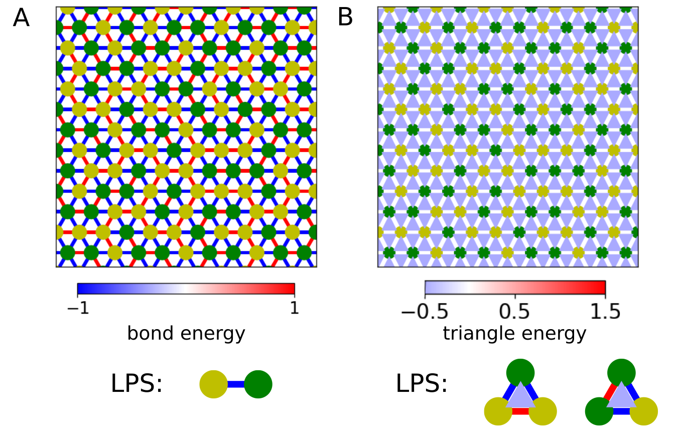
Figure 1: A. A ground state configuration of the antiferromagnetic Ising model on a triangular lattice (Equation 1). The color of sites indicates their state of spin. The color of bonds indicates their energy; blue bonds correspond to the locally preferred structure (LPS). Red bonds are defects due to frustration. B. The same configuration, now showing the energy of triangles as in Equation 2. All triangular plaquettes are in the LPS, and the model appears to be unfrustrated.

We start by examining what is probably the most popular example of frustrated system [7]: the antiferromagnetic Ising model on a triangular lattice (Figure 1). Its Hamiltonian reads

$$H=\sum_{i\sim j}s_{i}s_{j}$$ (1)

where the sum runs over all edges of the lattice, and $s_{i}=\pm 1$ are the local spin variables. The ground state energy per site of this model is $E_{0}=-1$ (Figure 1A). However, minimizing independently each term in the sum of Equation 1 would result in an energy per site of $E^{*}_{\mathrm{bonds}}=-3$, corresponding to each edge having an energy of $-1$. The “locally preferred order”, corresponding to antiparallel spins, is thus frustrated, as $E^{*}_{\mathrm{bonds}}<E_{0}$: it cannot be simultaneously achieved at all edges, due to the presence of triangles that overconstrain the system [8, 7]. A simple quantification of frustration in this model would thus be $f_{\mathrm{bonds}}=E_{0}-E^{*}_{\mathrm{bonds}}=2$, i.e. the difference between the energy per site in the ground state, and that in an ideal state where the preferred local order would be achieved everywhere. This frustration is generally invoked as the cause of the extensive degeneracy of the ground state of this system .

This definition is not without danger, however: indeed, consider the following rewriting of the Hamiltonian,

$$H=\sum_{\mathrm{triangles}\ (ijk)}\tau_{ijk}$$ (2)

where the sum runs over triangles of three bonds, and we define $\tau_{ijk}=\frac{1}{2}(s_{i}s_{j}+s_{j}s_{k}+s_{k}s_{i})$ as the energy of such a triangle. As each bond is part of two triangles, Equations 1 and 2 are clearly two equivalent ways of writing the same Hamiltonian. However, minimizing each term independently in Equation 2 now results in an energy per site of $E^{*}_{\mathrm{triangles}}=-1$, corresponding to each triangle having the minimum possible energy of $t_{ijk}=-1/2$ (Figure 1B). We thus have $f_{\mathrm{triangles}}=E_{0}-E^{*}_{\mathrm{triangles}}=0$: the Hamiltonian written in Equation 2 is unfrustrated, as its locally preferred order can tile the whole lattice. From this point of view, this system is extensively degenerate because it is underconstrained: as in some plaquette models, the simultaneous minimization of all terms of the Hamiltonian is not sufficiently constraining to select a single periodic ground state [7].

These two ways of writing the same Hamiltonian thus lead to different conclusions as to whether it is frustrated or not. Clearly, there is more information in Hamiltonian 1 in terms of the locality of the energy: Equation 2 is a less local way of writing the energy, and its energy density can be seen as an exact coarse-graining of the energy density of Equation 1, by averaging the energy of each triangle. Since this coarse-graining removes frustration, we can qualify this type of frustration of finite range, or irrelevant: it vanishes under renormalization. In order to quantify frustration in this system, one should therefore specify what scale is being considered: the antiferromagnetic Ising model on the triangular lattice is frustrated when going from the scale of a single bond to a triangle, but not from the scale of a triangle to the infinite lattice.

I.2 A minimal frustrated model?

We now discuss a second simplistic model that exhibits, we suggest, surprising frustration properties. Consider a triangular lattice where each bond carries a binary variable of orientation – pointing towards either of the two sites it connects (Figure 2A). We define the following Hamiltonian for this system:

$$H_{\mathrm{FNM}}=\sum_{i}\phi_{i}$$ (3)

where the local energy $\phi_{i}$ is the difference between the number of edges attached to $i$, pointing towards $i$, to the number of edges pointing against $i$ – i.e. the local flux at $i$. This is a specific instance of the $64$-vertex model [7]. The locally preferred structure corresponds to six edges pointing away from $i$ (Figure 2B), and tiling the lattice with such sites would result in an energy of $E^{*}_{\mathrm{site}}=-6$. This is however impossible, and ground state configurations include many defects to this ideal structure (Figure 2A): this system is frustrated.

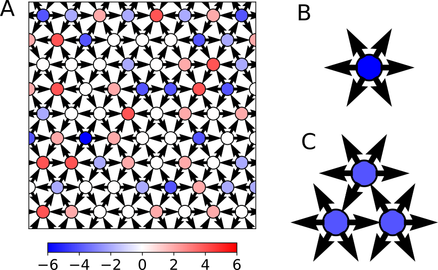
Figure 2: The “frustrated model” defined by Equation 3. The degrees of freedom are the orientation of the edges connecting two nodes. A. A typical ground state configuration. The color of each node indicates its energy $\phi_{i}$. B. The locally preferred structure at the scale of a single node has an energy $-6$. C. At the scale of three nodes, the LPS has energy $-4$ per site.

Grouping local energy variables together, as we did in Equation 2, reduces the frustration but does not cancel it: the locally preferred order at the scale of a triangle of three sites has energy per site $E^{*}_{\mathrm{triangles}}=-4$, still higher than the ground state (Figure 2C). This can be easily generalized to any cluster of sites: frustration in this model thus appears to be long-range, that is, it cannot be blurred out by a coarse-graining. This model has many peculiar properties, such as extensive degeneracy of the ground state, characterized for instance by the fact that the reversal of any closed loop of edge variables leaves the energy unchanged.

Rather than leading the reader further on, let us examine more closely the Hamiltonian proposed in Equation 3. Each edge contributes to two $\phi_{i}$ variables, each with an opposite sign: reversing its orientation thus displaces energy from one site to the other, but leaves the total energy unchanged – specifically, each edge variable has a zero contribution to the total energy, and thus Equation 3 can be rewritten exactly as

$$H_{\mathrm{FNM}}=0.$$ (4)

This model thus has the appearance of being frustrated, while being completely trivial – in a sense, it is a Frustrated Non-Model (FNM)… Admittedly, the Hamiltonian in Equation 3 is quite simple, and an aware reader could have realized that its frustration is only superficial. However, for an observer who only has access to the $\phi_{i}$ variables and the resulting field of local energies (Figure 2A), this is far from being obvious.

The field of local energies $\phi_{i}$ as defined here consists in what we define as an energy displacement, i.e. a configuration-dependent spatial patterning of the energy that always has zero sum, and thus no influence on the total Hamiltonian. Importantly, adding such an energy displacement to any non-trivial Hamiltonian would leave it unchanged: it would change “local energies”, but not the total energy of any state – and hence result in identical dynamical and thermodynamical properties. Two models that differ by a local energy displacement are thus physically and mathematically equivalent: their only difference lies in the way that the Hamiltonian is written in terms of local energies – a distinction that is arguably unphysical, and can be compared to a gauge change. However, as local energies are modified by energy displacements, they can affect the energy and even the nature of the locally preferred structure. This significantly complicates the problem of quantifying frustration. Indeed, any useful and physically meaningful definition of frustration should be gauge invariant and depend only on the Hamiltonian, not on the specific way that it is written – it should, in particular, see through Equation 3 and consider this model as non-frustrated, as its equivalent formulation in Equation 4 is trivial. Note that there is a scale to such energy displacements: as they change the local energies, they can also effectively change the range of interactions of the Hamiltonian. Indeed, in the case of the antiferromagnetic Ising model, going from Equation 1 to 2 can be seen as an energy displacement, moving the energy from the bonds to the triangles.

II Frustration of Local Energy Landscapes

In the previous section, we have identified two caveats that should be addressed in order to quantify geometrical frustration in a meaningful way. First, frustration should be a function of scale: as the structures considered get larger, the locally preferred structure will resemble more and more the ground state, as it internalizes constraints. Second, at a given scale, frustration should not depend on the specific way that the Hamiltonian is written – i.e. it should not be affected by a gauge change of the field of local energies, corresponding to local energy displacements. We now propose a framework to define and measure scale-dependent frustration. This framework relies on the classification of all possible local structures of the model at a given scale, and considering the ways to attribute an energy to each of them – i.e. the ways to define the Local Energy Landscape (LEL).

This approach is common in the study of supercooled liquids and glassy systems, where the idea of studying local structures is that a finite number of geometries can accurately describe the local environments of particles in a liquid: in supercooled liquids, distortions around local energy minima can be neglected in first approximation, and it makes sense to consider the energy of these local structures [10, 3, 11, 12]. This point of view is even more relevant in lattice models of discrete spins, in which the local structures are truly discrete: in such cases, models with short-range interactions can be exactly expressed in terms of their LEL, i.e. the energy associated to each possible local structures [13].

In this section, we first define the set of local structures corresponding to a given scale (Section II.1), and introduce the Local Energy Landscapes framework that maps structures onto local energies (Section II.2). We then show how to characterize the gauge of energy displacements that change the LEL, but not the total Hamiltonian (Section II.3). This allows us to propose a quantitative, gauge-invariant measure of frustration at a given scale (Section II.4). We then discuss the scale-dependence of this measure of frustration (Section II.5). Finally, we discuss a practical application of this method in the identification of ground state energies of spin systems (Section II.6). In each subsection, we first discuss concepts in their generality, then apply them to the practical case of triangular lattices.

Cluster
Size $z$	2	3	4	7	10	13	19
Number of LSs $n$	3	4	9 (10)	26 (28)	208 (352)	828 (1,400)	45,336 (87,600)
Energy displacements $\dim\Delta$	0	0	2	3 (3)	20 (37)	59 (103)	3504 (6753)

Table 1: High-symmetry local clusters on the triangular lattice, and the properties of corresponding local energy landscapes. Numbers in brackets correspond to chiral cases, i.e. considering enantiomeric structures as being distinct.

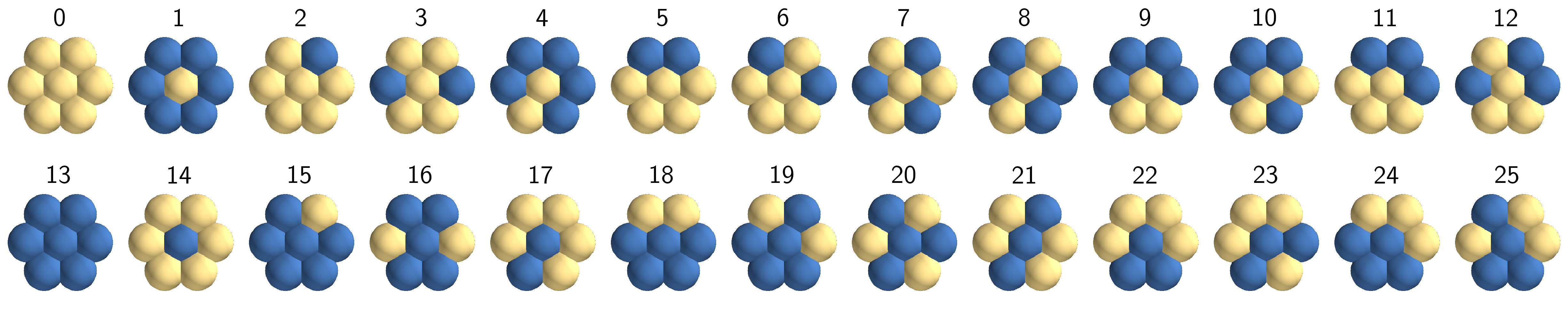
Figure 3: The $n=26$ distinct local structures corresponding to the coordination cluster with $z=7$ sites. The second row is spin-reversed compared to the first. Note that structures $12$ and $25$ are chiral; we treat both enantiomers as the same structure here. Distinguishing enantiomers would lead to two more local structures.

II.1 Local structures

We consider a system of $N$ binary spins on a Bravais lattice with periodic boundary conditions, in the limit of a large number of sites $N\to\infty$ where the effect of boundaries becomes irrelevant, and translation-invariant Hamiltonians with finite-range interactions on this spin system. All sites are thus equivalent, and can be characterized by their spin environment, with which they interact. To classify these environments, we first decide on a cluster of sites on which we will define local structures. This cluster should be larger than the interaction range of the Hamiltonian; the size $z$ of this cluster (the number of sites it contains) sets the scale at which we define and study frustration. It is convenient to use a cluster that has the highest possible symmetry, as this will limit the number of structures to consider. In Table 1 we present a selection of high-symmetry clusters on the triangular lattice. In most of this article, we will take the coordination shell cluster (one site and its six neighbors, $z=7$) as example to illustrate the concepts we discuss.

Having chosen a cluster of sites, we now introduce the set of all possible local structures on this cluster, i.e. the possible spin patterns on this cluster. There are $2^{z}$ distinct patterns, however if the Hamiltonian is isotropic (i.e. invariant under the discrete lattice rotations) it makes sense to consider two structures that differ by a rotation as identical. Depending on whether the considered Hamiltonian is chiral, one can choose to treat enantiomeric structures (i.e. non identical mirror copies) as distinct structures or not. Using these symmetries results in a set of $n$ distinct local structures. The values of $n$ corresponding to each cluster are presented in Table 1. In the case of the triangular coordination shell, the $n=26$ structures are depicted in Figure 3.

A spin configuration of the system can be described by its structural composition $\mathbf{c}$, an $n$-dimensional vector that specifies the fraction of sites in each local structure. The number of sites in structure $s$ is thus $N_{s}=Nc_{s}$ in this configuration. Note that a configuration is not fully characterized by its structural composition; conversely, as we will see, not all compositions are possible. Nevertheless, since the range of the Hamiltonian is shorter or equal than the size of the cluster we consider, the energy of a configuration is completely determined by the corresponding structural composition vector $\mathbf{c}$.

II.2 Local energy landscapes

We now introduce the local energy landscape (LEL) that relates the structural composition to the energy of the system. We associate an energy $\epsilon_{s}$ to each site in structure $s$, such the energy per site of the system reads

$$E(\mathbf{c})=\sum_{s=1}^{n}c_{s}\epsilon_{s}=\mathbf{c}\cdot\epsilon$$ (5)

where the vector $\epsilon=\{\epsilon_{s}\}_{s=1..n}$ is the LEL of the system. A vast class of popular models can be written exactly in such a form, which includes the Ising model, its variants with antiferromagnetic and/or next-to-nearest neighbor interactions, and plaquette models. The LEL thus fully characterizes the energetics of the system in terms of local structures. While structures are not energetically coupled in Equation 5, it is important to note that they are not independent: each spin is part of several structures, and these overlaps result in entropic coupling between structures. Indeed, the system’s free energy per site at temperature $T$ can be written (setting $k_{B}=1$) [13]:

$$F(T)=\min_{\mathbf{c},S(\mathbf{c})\geq 0}[\mathbf{c}\cdot\mathbf{\epsilon}-TS(\mathbf{c})]$$ (6)

where $S(\mathbf{c})$ is the entropy per site of a system with structural composition $\mathbf{c}$, which effectively counts the states available in the model compatible with these fractions of local structures. By convention we have $S(\mathbf{c})=-\infty$ if there are no states compatible with the structural composition $\mathbf{c}$ – for instance if it violates the basic constraints that all $c_{s}$’s are non-negative and that $\sum_{s}c_{s}=1$. The appeal of this approach lies in the fact that $S(\mathbf{c})$ depends only on the lattice geometry and the choice of cluster, not on the LEL. The thermodynamics of a broad class of models can thus be related, by Legendre transformation (Equation 6), to a single function $S(\mathbf{c})$. From this point of view, finding the ground state energy $E_{0}(\epsilon)$ of a model with LEL $\epsilon$ corresponds to finding the extremal point of definition of $S(\mathbf{c})$ along the direction $\epsilon$,

$$E_{0}(\epsilon)=\inf_{\mathbf{c},S(\mathbf{c})\geq 0}\mathbf{c}\cdot\mathbf{\epsilon}$$ (7)

which corresponds to the zero-temperature equilibrium state.

The minimum of $\epsilon$ corresponds to the minimal possible energy of a site, i.e. its energy when in the so-called Locally Preferred Structure (LPS). This energy is a lower bound to the ground state energy of the system:

$$E_{0}(\epsilon)\geq\min_{s=1\dots n}\epsilon_{s}$$ (8)

When there is equality, the system is unfrustrated at the scale of the structure considered: it can be uniformly tiled by locally preferred structures.

II.3 The gauge of energy displacements

The framework of local energy landscapes is significantly complicated by the fact that Equation 5 is not sufficient to define the LEL: two distinct local energy landscapes $\epsilon$ and $\epsilon^{\prime}$ can indeed correspond to the same physical system. This is the case if the difference between them, $\delta=\epsilon^{\prime}-\epsilon$, is an energy displacement, i.e. a non-zero LEL corresponding to a vanishing Hamiltonian. In this section, we show how to characterize the set $\Delta$ of possible energy displacements corresponding to a choice of local structures.

A LEL $\delta$ is an energy displacement if the energy of any possible configuration, as given by Equation 5, is zero: $\mathbf{c}\cdot\delta=0$ for all structural compositions $\mathbf{c}$ such that $S(\mathbf{c})\geq 0$. The set $\Delta$ of energy displacements $\delta$ thus has a vector space structure (a linear combination of energy displacements still corresponds to a zero Hamiltonian), which is a subspace $\Delta\subset\mathbf{R}^{n}$. A linear analysis of the entropy functional $S(\mathbf{c})$ around the infinite-temperature limit is sufficient to fully characterize this vector space. Indeed, one can write the following expansion for the entropy as a function of structural composition [14, 15, 13]:

$$S(\mathbf{c})=S_{\infty}-\frac{1}{2}(\mathbf{c}-\mathbf{c}^{\infty})\cdot\mathbf{C}^{-1}\cdot(\mathbf{c}-\mathbf{c}^{\infty})+O[(\mathbf{c}-\mathbf{c}^{\infty})^{3}]$$ (9)

where $S_{\infty}=\ln 2$ is the infinite-temperature entropy per site of a binary spin system. Here $\mathbf{c}^{\infty}$ is the structural composition at infinite temperature: in a fully random spin state, the proportion of sites in structure $s$ is $c^{\infty}_{s}=g_{s}/2^{z}$ where $g_{s}$ is the number of rotational variants of structure $s$ and $z$ is the number of sites in a structure [14]. The matrix $\mathbf{C}$ in Equation 9 relates to structural fluctuations at infinite temperature, and can be written as a covariance matrix,

$$C_{s{s^{\prime}}}=\frac{1}{N}\mathrm{Cov}_{T=\infty}(N_{s},N_{s^{\prime}})$$ (10)

for a large system of $N$ sites, where $N_{s}$ is the number of sites in structure $s$ in a given configuration. This matrix can either be obtained by simulations, or computed exactly by enumerating overlaps of structures [14, 13].

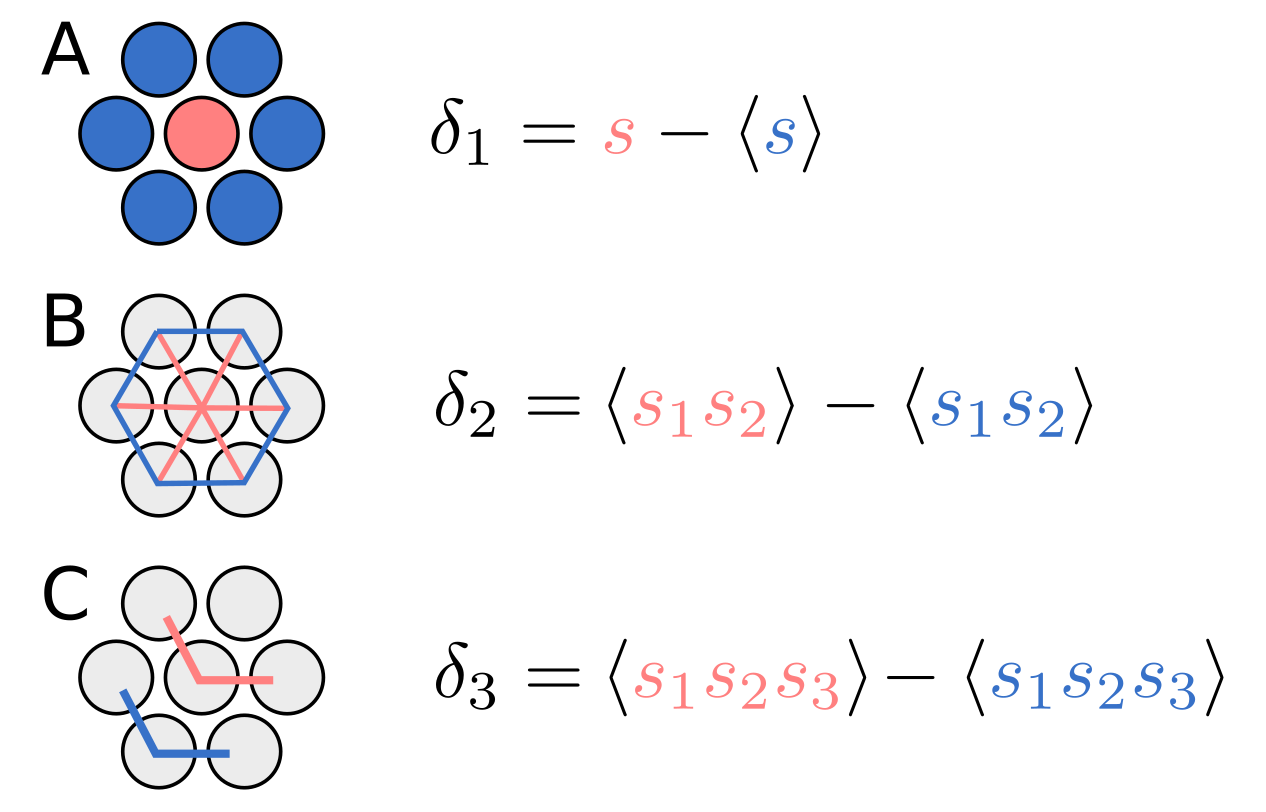
Figure 4: Schematic of the conserved quantities leading to the generators of the three-dimensional gauge space of energy displacements for the triangular coordination shell. A. Here $\delta_{1}$ is the difference between the spin value of the central site (red), to the average over its six neighbors (blue). This quantity is nonzero for all structures presented in Figure 3 except $0$ and $13$. However, the spatial average of the blue and the red term are both equal to the average spin value, for any configuration. Therefore, $\delta_{1}\cdot\mathbf{c}=0$ for all possible structural composition $\mathbf{c}$. B. Similarly, $\delta_{2}$ corresponds to the difference of two-spins interaction for radial edges (red) and lateral edges (blue) in the structure. While this can be locally nonzero, the spatial average of this quantity always vanishes. C. The last energy displacement corresponds to three-spin interactions that involve, or not, the central spin (averaged over all orientations).

Importantly, the matrix $\mathbf{C}$ typically has a non-trivial null space $\mathrm{Ker}(\mathbf{C})$, i.e. the set of eigenvectors associated to a zero eigenvalue. As Equation 9 involves $(\mathbf{c}-\mathbf{c}^{\infty})\cdot\mathbf{C}^{-1}\cdot(\mathbf{c}-\mathbf{c}^{\infty})$, we have $S(\mathbf{c})=-\infty$ for any composition $\mathbf{c}$ for which $\mathbf{c}-\mathbf{c}^{\infty}$ has a nonzero projection on $\mathrm{Ker}(\mathbf{C})$: the expansion of $S(\mathbf{c})$ “detects” forbidden configurations. The elements of $\mathrm{Ker}(\mathbf{C})$ correspond to the existence of conserved quantities. For instance, the constraint that $\sum_{s}c_{s}=1$ (i.e. that the set of structures is complete) implies that $(1,1,\dots,1)\in\mathrm{Ker}(\mathbf{C})$ for all choices of local cluster. In the case of the triangular coordination shell, there are also three non-trivial conservation laws, corresponding to redundancies in one-, two- and three-body interaction terms within the shell (see Figure 4 and caption). As a result, $\mathrm{Ker}(\mathbf{C})$ is four-dimensional for this choice of local cluster.

The space $\Delta$ of energy displacements corresponds to vectors that have $\delta\cdot\mathbf{c}=0$ for all “acceptable compositions” $\mathbf{c}$ such that $S(\mathbf{c})\geq 0$. As we have seen, these compositions are such that for any $\lambda\in\mathrm{Ker}(\mathbf{C})$, we have $\lambda\cdot(\mathbf{c}-\mathbf{c}^{\infty})=0$. The set of energy displacements thus corresponds to vectors $\delta$ that are both orthogonal to $\mathbf{c}^{\infty}$ and to all $(\mathbf{c}-\mathbf{c}^{\infty})$ for acceptable compositions $\mathbf{c}$. Mathematically, we thus have:

$$\Delta=\mathrm{Ker}(\mathbf{C})\cap\mathrm{Perp}(\mathbf{c}^{\infty})$$ (11)

with $\mathrm{Perp}(\mathbf{c}^{\infty})$ the hyperplane orthogonal to the vector $\mathbf{c}^{\infty}$, and $\mathrm{Ker}(\mathbf{C})$ the null space of $\mathbf{C}$. The exact values of both the covariance matrix $\mathbf{C}$ and the infinite-temperature composition $\mathbf{c}^{\infty}$ are analytically accessible; Equation 11 thus provides an operational way to classify energy displacements for a given definition of local structures. In Table 1, we indicate the dimensionality of the vector space $\Delta$ for all choices of local cluster. All clusters except the smallest ones admit energy displacements.

To summarize, the space $\Delta$ of energy displacements acts as a gauge group for the definition of local energy landscapes: for $\delta\in\Delta$, the landscapes $\epsilon$ and $\epsilon+\delta$ are physically equivalent, as they correspond to the same Hamiltonian.

II.4 A gauge invariant definition for frustration

We now examine the influence of energy displacements on the quantification of frustration. As discussed in Section I.1, one should first specify the scale $z$ at which we define it, corresponding to the number of sites in the cluster used to define the local energy landscape. The idea of frustration as the incompatibility between the Locally Preferred Structure (LPS) and filling space can be intuitively quantified by the difference between the energy of a site in the LPS, i.e. the local energy landscape minimum $\min_{s}\epsilon_{s}$, and the average energy per site in the ground state $E_{0}$. This quantity, however, is not gauge invariant: two energy landscapes corresponding to the same Hamiltonian may have different minima. In particular, arbitrarily large “apparent frustration” can be produced by adding a large energy displacement to any LEL, as we made evident in Section I.2.

We thus argue that the pertinent way to quantify the frustration of a Hamiltonian is to minimize it over the gauge group $\Delta$. This way, a system will be considered unfrustrated if it admits a LEL representation $\epsilon^{*}$ such that $\min_{s}\epsilon^{*}_{s}=E_{0}$. If it does not, then the system is frustrated, and the smallest gap $f_{z}$ between the ground state energy and the energy of the LPS quantifies frustration at scale $z$:

$$f_{z}(\epsilon)=E_{0}(\epsilon)-\max_{\delta\in\Delta}\left[\min_{s=1\dots n}(\epsilon_{s}+\delta_{s})\right]$$ (12)

Here $f_{z}(\epsilon)$ is a non-negative quantity, and the optimization over $\delta$ ensures that it is gauge invariant. Note that the quantity $\min_{s}(\epsilon_{s}+\delta_{s})$, corresponding to the LPS energy of the LEL $\epsilon+\delta$, is a linear-by-parts, concave function of $\delta$: the maximization in Equation 12 is thus non-ambiguous (there are no local maxima). While this optimization might not be tractable analytically, it can be efficiently performed numerically with algorithms such as the Nelder-Mead simplex .

In Equation 12, the LEL $\epsilon^{*}=\epsilon+\delta$ that maximizes the LPS energy plays a special role. It typically has at least two distinct, degenerate LPS: indeed, as the LPS energy is maximal, it should be such that no further energy displacement can increase the energy of a LPS without also decreasing the energy of the other.

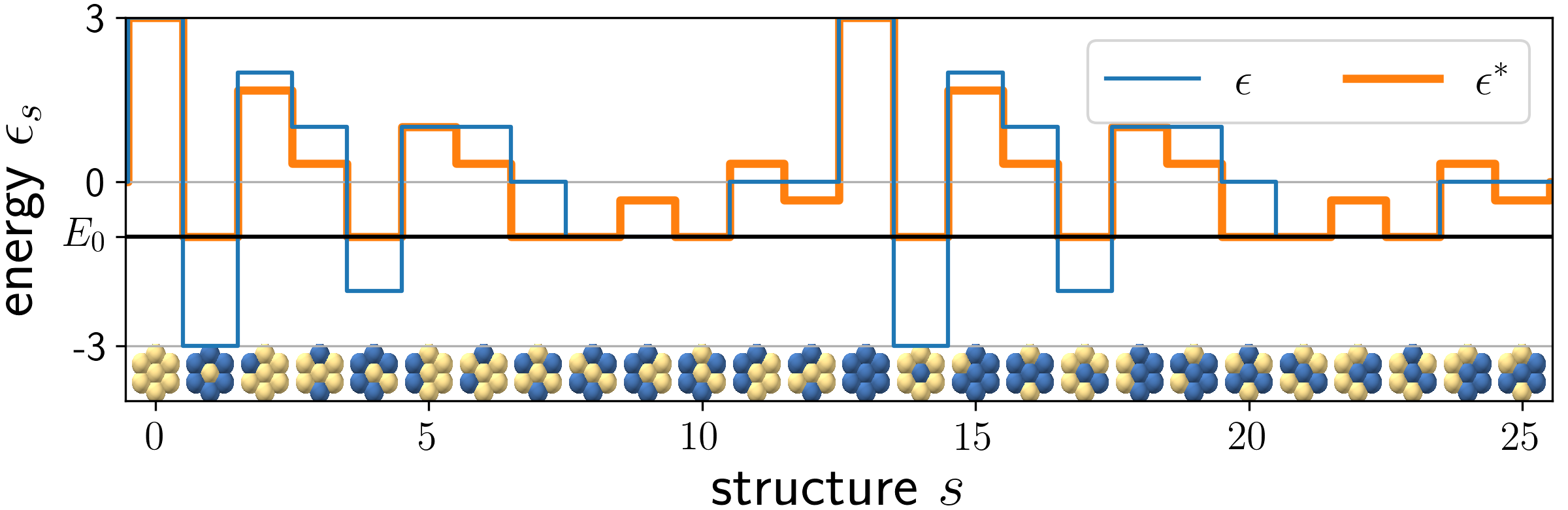
Figure 5: Two equivalent local energy landscapes, at the scale of the coordination shell, for the antiferromagnetic Ising model. Blue: the local energy is $\frac{1}{2}s_{i}\sum_{j\sim i}s_{j}$, which corresponds to taking into account the energy of the radial bonds connecting $i$ to its neighbors. The local structures $1$ and $14$ are locally preferred, with energy $-3$, to compare with the ground state energy $E_{0}=-1$. Orange: the optimal LEL for this model, as defined by Equation 12. The LPS is largely degenerate (1, 4, 7, 8, 10 and their spin-reversed variants), and all have energy $-1$, equal to the ground state energy. Any configuration composed exclusively of these structures is a ground state configuration; as many such configurations exist, the ground state is extensively degenerate.

We now apply our quantitative definition of frustration (Equation 12) to specific models. In Figure 5, we consider the antiferromagnetic Ising model, and compare $\epsilon^{*}$ with an usual local energy landscape representation of the Hamiltonian. As we discussed in Section I.1, this model only has finite-range frustration: already at the scale of a three-sites triangle, the model can be written in a frustration-free manner (Equation 2). Our approach consistently finds that this is also true at the scale of the coordination shell: $f_{7}=0$.

Table 2: Frustration analysis of the Favoured Local Structures (FLS) model. Each line corresponds to a Hamiltonian where sites in the selected local structure – the FLS – are attributed an energy $-1$, while all other sites have zero energy. We consider all 13 distinct structures on the triangular lattice coordination shell (Figure 3, the other 13 being equivalent through spin inversion). We identify ground state structures and their energies $E_{0}$ using the systematic search algorithm described in Ref. [17]. The plots show two equivalent LEL representations of the Hamiltonian on the coordination shell cluster: its original definition as a delta-peaked LEL (blue dashes), and $\epsilon^{*}$, (one of) the LEL with highest minimal energy (orange line). We finally indicate the frustration defined in Equation 12 at the scale of three different clusters. This optimization is performed using the SciPy implementation of the Nelder-Mead algorithm [18].

ID	FLS	Ground state	$E_{0}$	Cell size	Local energy landscape	$f_{7}$	$f_{10}$	$f_{13}$
0			$-1$	$1$		$0$	$0$	$0$
1			$-0.3333$	$3$		$0$	$0$	$0$
2			$-0.8571$	$7$		$0$	$0$	$0$
3			$-0.75$	$4$		$0$	$0$	$0$
4			$-0.4$	$5$		$0$	$0$	$0$
5			$-0.6667$	$3$		$0$	$0$	$0$
6			$-0.6667$	$9$		$0.0833$	$0$	$0$
7			$-0.6667$	$3$		$0$	$0$	$0$
8			$-0.5$	$2$		$0$	$0$	$0$
9			$-0.4444$	$27$		$0.0171$	$0.0171$	$0$
10			$-0.5$	$4$		$0$	$0$	$0$
11			$-0.5$	$12$		$0.0455$	$0$	$0$
12			$-0.6$	$10$		$0$	$0$	$0$

A more complex class of models is presented in Table II.4: the Favoured Local Structures (FLS) model. This model is defined directly through its local energy landscape, which is delta-peaked to favor a single structure (the FLS, with energy $-1$) while all others have zero energy. We have previously studied this model on two- [19] and three-dimensional [17] lattices, revealing that the geometry of the FLS controls a surprisingly rich phenomenology, including complex crystalline ground states [17], liquid-liquid transitions [15, 20], and slow dynamics [20, 17]. In Table II.4, we summarize results for the variant of this model where local structures are defined on the coordination shell . Twelve of the thirteen distinct choices of FLS (the exception being the trivial all-up case, labelled 0) result in non-trivial ground states with $E_{0}>-1$ (i.e. including non-FLS defects), and would thus be traditionally tagged as frustrated. However, applying our formalism to each local energy landscape, we find that in nine of these twelve systems, frustration has a finite range and vanishes at the scale of the coordination shell itself: $f_{7}=0$. While these systems appear frustrated, they are thus completely equivalent to models with the same interaction range, but for which there are multiple minima to the LEL, and a combination of them can tile the lattice perfectly. The remaining three systems (corresponding to structures 6, 9 and 11) have nonzero $f_{7}$, although the numerical values for this frustration parameter (respectively $1/12$, $2/117$ and $1/22$) are substantially smaller than the gap between the FLS energy and the ground state energy in the initial formulation of the problem (respectively $1/3$, $5/9$ and $1/2$). Thus even in the FLS model, a model explicitly built to study geometrical frustration of local structures, most systems that are apparently frustrated do not resist a closer investigation: our gauge-invariant algorithm to quantify frustration shows that frustration is an exception, rather than the norm.

II.5 The range of frustration

Our quantitative definition of frustration (Equation 12) depends on the size $z$ and geometry of the cluster on which we define the LEL. This cluster must be at least as large as the range of interactions of the Hamiltonian; it can however be larger. Hierarchically increasing the cluster size by including more sites, as in the sequence shown in Table 1, gives access to more energy displacements, which are less local as they displace energy over a longer range. The optimization in Equation 12 thus occurs on a higher dimensional space when $z$ increases; as a result, $f_{z}$ is a non-increasing function of $z$ when considering a hierarchical family of clusters.

Our formalism thus distinguishes two classes of frustrated systems:

• systems with finite-range frustration have a characteristic size $z^{*}$ such that $f_{z^{*}}=0$. This size corresponds to the scale at which the Hamiltonian can be written in an unfrustrated manner, i.e. such that locally preferred structures can tile the whole space. At this scale, the locally preferred structures are typically degenerate, which can result in a degeneracy of the ground state of the system. Geometrical constraints are localized at scales $z\leq z^{*}$, and can be eliminated by an exact coarse-graining step.

• systems with long-range frustration have a nonzero $f_{z}$ at all scales: there is no way to write them in terms of finite-range unfrustrated LEL. Such systems would thus have truly non-local geometrical constraints. Stability of the ground state implies that the frustration function still decreases with scale, with an upper bound $f_{z}<A/z^{1/d}$ where $d$ is the dimension of space .

On the triangular lattice, we have seen that the antiferromagnetic Ising model has finite-range frustration with $z^{*}=3$ (Equation 2), while nine of the twelve frustrated FLS models have $z^{*}=7$ (Table II.4). Interestingly, we find that the remaining three choices of FLS have finite-range frustration too, with $z^{*}=10$ for FLSs $6$ and $11$, and $z^{*}=13$ for FLS $9$. Note that these structures correspond to most of those for which the crystalline ground state has the largest elementary cell (respectively $9$, $27$ and $12$). Thus, none of the systems defined by a FLS on the triangular lattice coordination shell have long-range frustration. Extending this study to the case of a chiral Hamiltonian (i.e. favoring only structure 12, but not its enantiomer) and to the case of structures defined on the empty shell (with a cluster including the six neighbors of a site, but not the site itself, as studied in Refs. [19, 15, 20]) does not change this conclusion: all 2D binary spin systems studied by the authors have $z^{*}\leq 13$, and thus have finite-range frustration only. At the time of this writing, it remains unclear whether there exists discrete spin systems with long-range frustration.

A practical constraint to the investigation of more complex structures (e.g. with more than two spin values, or on three-dimensional lattices) is that the number $n$ of structures grows exponentially with $z$. The energy displacements are obtained as the null space of the $n\times n$ matrix $\mathbf{C}$; we conjecture that their number grows exponentially too (Table 1). This puts sharp constraints on the size at which it is possible to study frustration with our method; in particular, any type of scaling analysis is impossible for now. This might not be hopeless, though: in this article, our search through the energy displacement space is blind. Identifying in advance what energy displacement will matter could allow to estimate $f_{z}$ without having to perform the high-dimensional optimization. We leave this possibility open for future work.

II.6 Provability of ground states

To finish on a brighter note, we present a practical application of our framework in the identification of ground state energies. Computing the ground state energy of a many-body spin Hamiltonian such as the FLS models (Table II.4) is a challenging problem, even if their interactions are short-ranged. In practice, we have found that constructive, enumerative techniques permit to investigate all possible crystalline structures up to a given cell size, using an adaptation of the algorithm developed by Hart and Forcade [23, 17]. This algorithm typically provides a “good candidate” for the ground state structure. However, it is difficult to know for sure that this candidate is, indeed, the ground state: how to be sure that no structure with a larger, more complex unit cell and a slightly lower energy exists?

Our framework provides lower bounds to this ground state energy: the LPS energy of any LEL representation of the Hamiltonian (Equation 8). In particular, for a given cluster size $z$ on which we define the LEL, the most restrictive bound is

$$E^{*}_{z}(\epsilon)=\max_{\delta\in\Delta}\left[\min_{s=1\dots n}(\epsilon_{s}+\delta_{s})\right]$$ (13)

i.e. the maximal LPS energy in Equation 12. When this energy $E^{*}_{z}(\epsilon)$ coincides with the energy of a crystalline state that could be constructed with, e.g., our enumerative algorithm, it means that the system has finite-range frustration. Furthermore, it provides a rigorous proof that this state is, indeed, the ground state of the system. As all FLS systems presented in Table II.4 have finite-range frustration, we thus have proven that the crystalline structures depicted in this table are, indeed, ground state configurations. This also applies to the variant of the model studied in Refs. [19, 15, 20].

Interestingly, this method of “proving ground state energies” would not work for systems with long-range frustration (if such systems exist). This could mean that these systems effectively belong to a different class of complexity for the provability of their ground states.

III Discussion

In this article, we have examined the notion of geometrical frustration in the context of lattice spin models with short-range interactions and translation invariance. This notion is understood here as the impossibility for the locally preferred order to tile space. To sharpen this idea of locally preferred order, we introduce the framework of local energy landscapes, which associates an energy to each spin depending on its local spin environment – i.e. its local structure. There is, however, an ambiguity in this choice: for a given Hamiltonian, we have seen that there are typically many equivalent ways to define a local energy landscape, related by unphysical gauge changes that we term energy displacements. We have shown how to characterize the gauge group, and construct it in practical cases, using a high-temperature expansion of the entropy. This allows us to define a gauge invariant measure for frustration, which depends only on the Hamiltonian and the scale considered. The scale-dependence of this frustration function defines two classes of frustrated systems. When frustration vanishes above a certain scale, we say that the system has finite-range frustration: it can be eliminated by a local “blurring” of the local energy. All systems studied in this article fall in this class; in such cases, our framework provides a rigorous proof that our estimate of the minimum energy is indeed the ground state of these systems. We speculate that a second class of systems, that we term long-range frustrated, exists. For such systems, the geometrical constraints in their organization are non-local, which might lead to interesting physical properties; however, an example of spin system with long-range frustration remains to be discovered.

The key difficulty in this assessment of geometrical frustration is that it requires a notion of local energy, which is typically ambiguous: only the global Hamiltonian has a true physical meaning. The gauge of energy displacements, that we have characterized here in the case of spin systems, reflects this ambiguity: two local energy landscapes related by an energy displacement are virtually indistinguishable. This has practical consequences: any attempt to infer the LEL from experimental measurements of the statistics of structures would be unable to resolve such difference, and would thus yield ambiguous results. Our framework resolves this ambiguity. Other approaches attempting to attribute energies to local structures, for instance in particle systems in the study of icosahedral structures [10, 3, 12] or other clusters [24], might be subject to such ambiguity too. Our framework could be adapted to such systems, and provide a route towards a quantitative measure of frustration. This is, we argue, a necessary step towards connecting geometrical frustration to its alleged consequences, such as the extensive degeneracy of ground states or slow dynamics in the supercooled liquid.

Finally, we note that we have only considered bulk systems here, for which there is no need to specify boundary conditions. This is the relevant case for the thermodynamic properties of liquids, crystals and glasses. However, there has been recently an emergent interest in the physical properties of geometrically frustrated systems with free boundaries, such as assembling proteins or filaments in a dilute solution [25, 26]. In this “geometrically frustrated assembly” paradigm, frustration in the bulk competes with surface tension at the free surface. In order to apply our framework to these systems, one would thus need to consider the influence of energy displacements on the surface tension.