Ghost Dark Energy Model in $f(G)$ Gravity

Abstract

In this paper, we investigate cosmological consequences of ghost dark energy model in modified Gauss-Bonnet gravity. We construct ghost dark energy $f(G)$ model by using correspondence scenario for both interacting and non-interacting schemes. For this purpose, we consider FRW universe with pressureless matter and power-law scale factor. We examine the behavior of equation of state parameter and check the stability of ghost dark energy model through squared speed of sound parameter. We also analyze the behavior of phase planes like $\omega_{eff}-\omega^{\prime}_{eff}$ and $r-s$ graphically. It is found that the equation of state parameter represents quintessence era for non-interacting while phantom phase of the universe for interacting case. The squared speed of sound indicates stable ghost dark energy model for both cases. The $\omega_{eff}-\omega^{\prime}_{eff}$ plane shows thawing region for non-interacting while freezing region for interacting case. The $r-s$ plane corresponds to Chaplygin gas model in both scenarios. We conclude that ghost dark energy model describes evolution of the universe for appropriate choice of parameters.

Keywords: Ghost dark energy; Cosmological evolution; $f(G)$ gravity.
PACS: 04.50.Kd; 95.36.+x.

1 Introduction

The well-known phenomenon of accelerated expansion of the universe is usually explained by the exotic type force known as dark energy (DE). The cosmological constant is the simplest DE model and is the base of $\Lambda$CDM model. Despite showing the consistent behavior with all observational data, $\Lambda$CDM model undergoes several difficulties like fine tuning and cosmic coincidence problem [1]. In order to substantiate the behavior of DE, researchers used two different approaches, firstly the dynamical DE models [2] and secondly the modified gravity theories [3].

A dynamical DE model, known as Veneziano ghost DE (GDE) has been introduced in late $70$’s by Veneziano [4]. This has significant non-trivial physical properties for the expanding universe or in spacetime having non-trivial topological formation. The existence of Veneziano GDE is supposed to resolve $U(1)$ problem [5]. The GDE has little contribution to the vacuum energy density in a curved spacetime. It is proportional to $\Lambda^{3}_{QCD}H$, where $\Lambda_{QCD}$ and $H$ are the quantum chromodynamics (QCD) mass scale and Hubble parameter, respectively [6]. For measures $\Lambda_{QCD}\sim 100MeV$ and $H\sim 10^{-33}MeV$, $\Lambda^{3}_{QCD}H$ gives approximately $(10^{-3}eV)^{4}$ to the observed DE density. This numeric value is incredible to offer the necessary exotic force for accelerating universe and also alleviates the fine tuning problem.

The Gauss-Bonnet (GB) theory is incredibly motivating theory as it shows consistent behavior with solar system constraints. The GB invariant has the expression as $G=R_{\alpha\rho\delta\sigma}R^{\alpha\rho\delta\sigma}-4R_{\alpha\rho}R^{\alpha\rho}+R^{2}$, where $R$, $R_{\alpha\rho}$ and $R_{\alpha\rho\delta\sigma}$ stand for the Ricci scalar, Ricci tensor and Riemann curvature tensor, respectively. This invariant is a four-dimensional topological expression with restriction for spin-2 ghost instability. Nojiri and Odintsov [7] proposed $f(G)$ gravity by adding a generic function in the Einstein-Hilbert action. This amazing theory effectively describes the early and late-time cosmic evolution. Cognola et al. [8] studied DE model in modified GB gravity to discuss cosmological evolution and also addressed the issues of hierarchy problem. Nojiri et al. [9] discussed DE in two scenarios, one for implicit equation of state (EoS) of the universe and other for modified GB gravity. They predicted the natural transition from early to late-time universe. De Felice and Tsujikawa [10] analyzed consistency of the $f(G)$ model with solar system constraints.

The current accelerated expansion of the universe can be investigated by many DE models. Setare and Saridakis [11] explored the condition under which the holographic and GB DE models describe the accelerated expansion of the universe. They also studied the correspondence of holographic DE model with quintom, phantom and canonical models and highlighted stable results for the accelerated universe [12]. Later, Setare et al. [13] implemented this concept of correspondence to different DE models and modified theories. Sheykhi and Movahed [14] discussed implications of the interacting GDE model in general relativity and observed expansion of the universe using constraints on the model parameter. Sadeghi et al. [15] explored the interacting GDE models by varying $G$ as well as $\Lambda$. They computed EoS and deceleration parameters numerically to analyze the behavior of the universe.

The reconstruction phenomenon in modified theories of gravity is a useful technique to develop a viable DE model that anticipates the history of cosmic evolution. This reconstruction scenario compares the corresponding energy densities of DE model and modified theory of gravity. In this scheme, we derive the modified generic function of underlying theory through correspondence technique of energy densities. Much work have been carried out in cosmology using this scenario of correspondence for different DE models.

Saaidi et al. [16] reconstructed the GDE $f(R)$ model using correspondence scheme and analyzed its stability as well as evolution by evaluating cosmological parameters. Alavirad and Sheykhi [17] studied cosmological constraints on GDE for FRW universe using interaction between DE and dark matter in Brans-Dicke theory. Fayaz and his collaborators [18] investigated this model by considering Bianchi-I universe in $f(R)$ gravity and analyzed the cosmic evolution of the corresponding model. Chattopadhyay [19] explored stability of cosmic evolution using cosmological parameters. Fayaz et al. [20] investigated this model in $f(R,T)$ gravity for Bianchi-I universe and concluded that their results favor the current behavior of the universe.

The $f(G)$ gravity is an interesting modified gravity theory which helps to better understand current and late-time acceleration of the universe. Zhou et al. [21] analyzed cosmological constraints of DE model based on the modified GB gravity and derived the condition of viability for the model with cosmic trajectories that mimics the $\Lambda$CDM limit for both radiation as well as matter dominant eras. Sheykhi and Bagheri [22] explored quintessence GDE model to describe recent evolution of the cosmos. Chattopadhyay [23] analyzed the generalized second law of thermodynamics in QCD ghost $f(G)$ gravity. Shamir [24] discussed viable DE models in $f(G)$ gravity showing consistent behavior for the expansion of the universe.

In this paper, we use correspondence scenario to reconstruct GDE $f(G)$ model and examine the EoS parameter, squared speed of sound parameter and phase planes. The format of the paper is as follows. In the next section, we adopt reconstruction procedure for GDE $f(G)$ model. Section 3 investigates evolution of the universe for non-interacting case while section 4 examines the interacting GDE $f(G)$ model. Finally, we discuss our results in the last section.

2 Reconstruction of GDE $f(G)$ Model

In this section, we apply the correspondence between GDE and $f(G)$ gravity to reconstruct GDE $f(G)$ model. The action of $f(G)$ gravity is defined as [25]

$$S=\int d^{4}x\sqrt{-g}\left(\frac{R}{2\kappa^{2}}+f(G)+\mathcal{L}_{m}\right),$$ (1)

where $\kappa^{2}=1$ and $\mathcal{L}_{m}$ are the coupling constant and matter Lagrangian density, respectively. The corresponding field equations are

$$R_{\alpha\beta}-\frac{1}{2}Rg_{\alpha\beta}=T_{\alpha\beta}^{eff},$$ (2)

where $T_{\alpha\beta}^{eff}$ is the effective energy-momentum tensor given by

$$T_{\alpha\beta}^{eff} = \kappa^{2}T^{(m)}_{\alpha\beta}-8[R_{\alpha\rho\beta\gamma}+R_{\rho\beta}g_{\gamma\alpha}+R_{\alpha\gamma}g_{\beta\rho}-R_{\gamma\rho}g_{\beta\alpha}-R_{\alpha\beta}g_{\rho\gamma}$$ (3)

$$+ \frac{1}{2}R(g_{\alpha\beta}g_{\rho\gamma}-g_{\rho\gamma}g_{\alpha\beta})]\nabla^{\rho}\nabla^{\gamma}f_{G}-(Gf_{G}-f)g_{\alpha\beta},$$

where $f_{G}=\frac{df}{dG}$. Also, $\nabla_{\alpha}$ and $T^{(m)}_{\alpha\beta}$ represent the covariant derivative and matter energy-momentum tensor, respectively. The field equations for FRW universe model in the presence of perfect fluid take the form

$$3H^{2}=\rho_{m}+\rho_{DE},\quad-(2\dot{H}+3H^{2})=P_{m}+P_{DE},$$ (4)

where dot represents the time derivative and subscript $m$ denotes matter contribution of energy density as well as pressure. The energy density and pressure of dark source terms are

$$\rho_{DE} = \frac{1}{2}(Gf_{G}-f-24^{2}H^{4}(2\dot{H}^{2}+H\ddot{H}+4H^{2}\dot{H})f_{GG}),$$ (5)

$$P_{DE} = \frac{1}{2}(8H^{2}\ddot{f_{G}}+16H(H^{2}+\dot{H})\dot{f}_{G}-Gf_{G}+f),$$ (6)

where $G=24H^{2}(H^{2}+\dot{H})$.

The first field equation leads to

$$\Omega_{m}+\Omega_{DE}=1,$$ (7)

where $\Omega_{m}=\frac{\rho_{m}}{3H^{2}}$ and $\Omega_{DE}=\frac{\rho_{DE}}{3H^{2}}$ are the fractional energy densities associated with matter and dark source, respectively. Dynamical DE models whose energy density is proportional to Hubble parameter play a vital role in explaining accelerated expansion of the universe. The GDE model is one of the dynamical DE model whose energy density is defined as [26]

$$\rho_{GDE}=\alpha H,$$ (8)

where $\alpha$ is an arbitrary constant having dimension $[energy]^{3}$. We establish the correspondence between GDE and $f(G)$ model by equating corresponding densities. Using Eqs.(5) and (8), it follows that

$$Gf_{G}-f-24^{2}H^{4}(2\dot{H}^{2}+H\ddot{H}+4H^{2}\dot{H})f_{GG}=2\alpha H.$$ (9)

In order to obtain the analytic solution of this equation, we consider the following form of scale factor as

$$a(t)=a_{0}t^{m},$$ (10)

where $a_{0}$ is a constant representing the present day value of the scale factor. Using Eq.(10) in (9), we obtain

$$G^{2}f_{GG}+\frac{m-1}{4}Gf_{G}-\frac{m-1}{4}f=\frac{\alpha m^{\frac{1}{4}}(m-1)^{\frac{3}{4}}G^{\frac{1}{4}}}{2^{\frac{7}{4}}3^{\frac{1}{4}}},$$ (11)

which is a second order linear differential equation whose solution is

$$f(G)=c_{1}G^{\frac{1}{4}(1-m)}+c_{2}G-\frac{\alpha(m-1)^{\frac{3}{4}}G^{\frac{1}{4}}2^{\frac{9}{4}}}{3^{\frac{5}{4}}m^{\frac{3}{4}}},$$ (12)

where $c_{1}$ and $c_{2}$ are integration constants. This represents the reconstructed GDE $f(G)$ model. Using Eq.(12) in (5) and (6), we have

$$\rho_{DE} = \frac{\alpha m^{\frac{1}{4}}G^{\frac{1}{4}}}{2^{\frac{3}{4}}3^{\frac{1}{4}}(m-1)^{\frac{1}{4}}},$$ (13)

$$P_{DE} = \frac{\alpha G^{\frac{1}{4}}(1-3m)}{2^{\frac{3}{4}}3^{\frac{5}{4}}m^{\frac{3}{4}}(m-1)^{\frac{1}{4}}},$$ (14)

where $m\neq 1$. The graphical analysis of reconstructed GDE $f(G)$ model against $G$ is shown in Figure 1. We take $c_{1}=8.5$, $c_{2}=8.5$, $\alpha=22.05$, $\rho_{m_{0}}=0.23$, $a_{0}=1$, $\Omega_{m_{0}}=0.313$ and $H_{0}=67.48$ throughout the analysis. It is observed that the reconstructed $f(G)$ model initially exhibits rapidly decreasing behavior and then gradually increases as $G$ increases in the range $1\leq m\leq 3$.

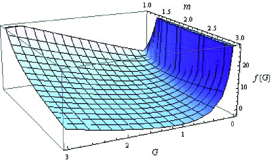
Figure 1: Plot of $f(G)$ for $\alpha=22.05$, $\Omega_{m_{0}}=0.313$ and $H_{0}=67.48$.

3 Non-Interacting GDE $f(G)$ Model

Here, we study non-interacting scenario of cold dark matter and GDE. The conservation equations corresponding to matter and dark source terms for pressureless fluid $(P_{m}=0)$ are

$$\dot{\rho}_{m}+3H\rho_{m}=0,$$ (15)

$$\dot{\rho}_{DE}+3H\rho_{DE}(1+\omega_{DE})=0.$$ (16)

Equation (15) has solution of the form

$$\rho_{m}=\rho_{m_{0}}a^{-3},$$ (17)

where $\rho_{m_{0}}$ is an arbitrary constant.

In the following, we investigate the evolution of EoS parameter, squared speed of sound and cosmological planes.

3.1 The EoS Parameter

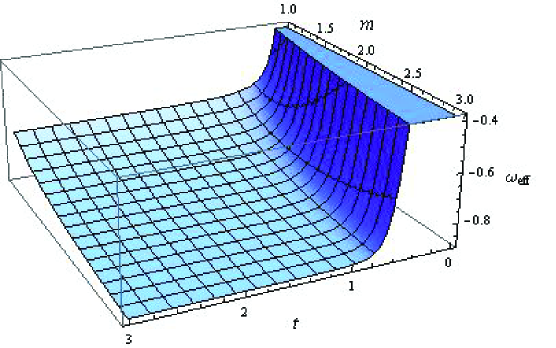
Figure 2: Plot of EoS parameter for $\alpha=22.05$, $\rho_{m_{0}}=0.23$, $a_{0}=1$, $\Omega_{m_{0}}=0.313$ and $H_{0}=67.48$.

The EoS parameter is given by

$$\omega_{eff}=\frac{P_{eff}}{\rho_{eff}}=\frac{P_{DE}}{\rho_{DE}+\rho_{m}}.$$ (18)

Using Eqs.(13), (14) and (17) in the above equation, we have

$$\omega_{eff} = \frac{-3m+1}{3m+\frac{3\rho_{m_{0}}t^{1-3m}}{\alpha a_{0}^{3}}}.$$ (19)

Figure 2 shows graphical behavior of this parameter for $1<m\leq 3$. We observe that the EoS parameter presented quintessence era and approaches the phantom divide line but never crosses it for $m>1$ as $t$ increases. As the universe will collapse in the absence of DE, thus the existence of DE elaborates our current accelerating expansion of the universe. This shows that the GDE $f(G)$ model favors DE phenomenon.

3.2 Squared Speed of Sound Parameter

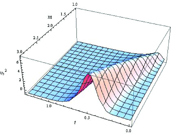
Figure 3: Plot of squared speed of sound parameter for $\alpha=22.05$, $\rho_{m_{0}}=0.23$, $a_{0}=1$, $\Omega_{m_{0}}=0.313$ and $H_{0}=67.48$.

We compute this parameter to analyze the stability of GDE $f(G)$ model. It has the following expression

$$\nu_{s}^{2}=\frac{\dot{P}_{eff}}{\dot{\rho}_{eff}}.$$ (20)

The sign of $\nu_{s}^{2}$ helps to determine stability of the reconstructed DE model. A positive signature of $\nu_{s}^{2}$ designates stability of the model whereas its negative value highlights the instability. Using Eqs.(13) and (14) in (20), it follows that

$$\nu_{s}^{2} = \frac{(1-3m)\alpha a_{0}^{3}m}{3m^{2}\alpha a_{0}^{3}+\rho_{m_{0}}t^{1-3m}}(1+\frac{(1-3m)\rho_{m_{0}}t^{1-3m}}{3m^{2}\alpha a_{0}^{3}+\rho_{m_{0}}t^{1-3m}})$$

We plot the squared speed of sound for $m>1$ as shown in Figure 3. It is observed that $\nu_{s}^{2}>0$ throughout the evolution leading to the stable GDE $f(G)$ model.

3.3 The $\omega_{eff}-\omega^{\prime}_{eff}$ Plane

Caldwell and Linder [27] proposed $\omega_{eff}-\omega^{\prime}_{eff}$ plane to analyze the behavior of quintessence DE model. They classified the plane into two regions named as thawing ($\omega_{eff}<0,~{}\omega^{\prime}_{eff}>0$ ) and freezing regions ($\omega_{eff}<0,~{}\omega^{\prime}_{eff}<0$). Using Eq.(19), we have

$$\omega^{\prime}_{eff}=\frac{(1-3m)^{2}\rho_{m_{0}}t^{1-3m}\alpha a_{0}^{3}}{(3m^{2}\alpha a_{0}^{3}+\rho_{m_{0}}t^{1-3m})^{2}}.$$

Figure 4 exhibits the $\omega_{eff}-\omega^{\prime}_{eff}$ plane for GDE $f(G)$ model with three distinct values of $m$, i.e., $m=2,2.4$ and $2.8$. It is found that $\omega_{eff}-\omega^{\prime}_{eff}$ plane corresponds to thawing region for all considered values of $m$ showing a consistent behavior with our current accelerated expanding universe.

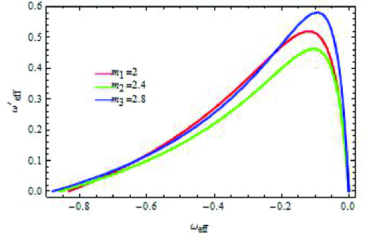
Figure 4: Trajectories of $\omega_{eff}-\omega^{\prime}_{eff}$ for GDE $f(G)$ model with GDE parameter $\alpha=22.05$, $\rho_{m_{0}}=0.23$, $a_{0}=1$, $\Omega_{m_{0}}=0.313$ and $H_{0}=67.48$.

3.4 The $r-s$ Plane

The accelerated expansion of the universe has been supported by various DE models that represent the same values for deceleration and Hubble parameters. These parameters fail to highlight the best among those models. In this regard, Sahni et al. [28] introduced two dimensionless parameters in terms of deceleration and Hubble parameters to classify DE models. These parameters are known as statefinder parameters defined as

$$r=\frac{\dddot{a}}{aH^{3}},\quad s=\frac{r-1}{3(q-\frac{1}{2})}.$$ (21)

The parameter $r$ can be expressed in terms of deceleration parameter as

$$r=2q^{2}+q-\acute{q}.$$ (22)

These parameters help to determine the distance of a certain DE model by using $\Lambda$CDM limit and also extricate the DE models. They classified the universe in different regions, e.g., CDM limit for $(r,s)=(1,0)$ and $\Lambda$CDM for $(r,s)=(1,1)$. Furthermore, the region ($r<1,s>0$) interprets the phantom and quintessence DE eras while the region $(s<0$, $r>1$) represents Chaplygin gas model. Using Eq.(19) in (21) and (22), we have

$$r = \frac{1}{2(3\alpha m^{2}a_{0}^{3}t^{3m}+\rho_{m_{0}}t)^{2}}(18t^{6m}\alpha^{2}m^{4}a_{0}^{6}-15t^{3m+1}\alpha m^{2}a_{0}^{3}\rho_{m_{0}}-27t^{6m}\alpha^{2}$$

$$\times m^{3}a_{0}^{6}+2t^{2}\rho_{m_{0}}^{2}+9t^{3m+1}m\alpha\rho_{m_{0}}a_{0}^{3}+9t^{6m}\alpha^{2}m^{2}a_{0}^{6}+27t^{3m}\alpha m^{3}\rho_{m_{0}}a_{0}^{3}$$

$$- 18t^{3m}\alpha m^{2}\rho_{m_{0}}a_{0}^{3}+3t^{3m}\alpha m\rho_{m_{0}}a_{0}^{3}),$$

$$s = \frac{3}{4(3\alpha m^{2}a_{0}^{3}t^{3m}+\rho_{m_{0}}t)^{3}}[(-1+3m)\alpha^{2}m^{2}a_{0}^{6}(\rho_{m_{0}}t^{6m}(9mt-9m^{2}+6m$$

$$- 3t-1)+3\alpha t^{9m}ma_{0}^{3}(3m-1))].$$

The trajectories of $r-s$ plane for GDE $f(G)$ model with $m=2,2.4$ and $2.8$ are shown in Figure 5. These plots show that the $r-s$ plane leads to the Chaplygin gas model regimes for all three values of $m$ and meet the CDM limit while $\Lambda$CDM limit cannot be obtained for the reconstructed model.

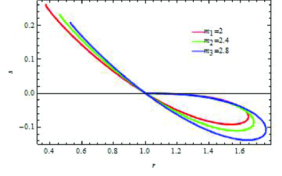
Figure 5: Trajectories of $r-s$ for GDE $f(G)$ model using $\alpha=22.05$, $\rho_{m_{0}}=0.23$, $a_{0}=1$, $\Omega_{m_{0}}=0.313$ and $H_{0}=67.48$.

4 Interacting GDE $f(G)$ Model

In this section, we investigate the interaction of GDE and pressureless dark matter. Ghost DE and dark matter violate the conservation equation while the interacting scenario leads to

$$\dot{\rho}_{m}+3H\rho_{m}=A,$$ (23)

$$\dot{\rho}_{DE}+3H\rho_{DE}(1+\omega_{DE})=-A,$$ (24)

where $A$ is the interaction which transfers energies between CDM and GDE. There are many simple choices like $3d_{1}H\rho_{DE}$, $3d_{1}H\rho_{m}$, and $3d_{1}H(\rho_{DE}+\rho_{m})$ to describe interaction in terms of energy densities and coupling constant $d_{1}$. Cai and Su [29] found that it is necessary for interaction term to change its sign for evolving the universe from deceleration to acceleration. However, the above three choices fail to obey this condition. Therefore, we choose a particular form of the interaction [30] as

$$A=3d_{1}H(\rho_{DE}-\rho_{m}),$$ (25)

which changes its sign to describe the evolution of the universe from deceleration to acceleration appropriately. Here, we analyze some cosmological parameters for interacting GDE $f(G)$ model.

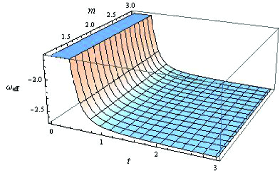
Figure 6: Plot of EoS parameter for $\alpha=22.05$, $\rho_{m_{0}}=0.23$, $a_{0}=1$, $d_{1}=0.3$, $\Omega_{m_{0}}=0.313$ and $H_{0}=67.48$.

The EoS parameter is found by substituting Eqs.(4) and (25) in (23) as follows

$$\omega_{eff} = (\frac{-3m+1}{3m}-d_{1}(\frac{-2}{\alpha t}+\frac{-3m+1}{3m}+2))(1+\frac{\rho_{m_{0}}t^{1-3m+3d_{1}}}{\alpha ma_{0}^{3}}$$ (26)

$$+ \frac{3md_{1}}{1-3m+3md_{1}})^{-1}.$$

Figure 6 illustrates graphical description of EoS parameter for $1<m<3$. It is observed that the EoS parameter shows phantom phase of the universe for $m>1$ as $t$ increases.

The corresponding squared speed of sound parameter is given by

$$\nu_{s}^{2} = (\frac{-3m+1}{3m}-d_{1}(\frac{-2}{\alpha t}+\frac{-3m+1}{3m}+2)+\frac{2d_{1}}{\alpha t})(1+\frac{\rho_{m_{0}}t^{1-3m+3d_{1}}}{\alpha ma_{0}^{3}}$$

$$+ \frac{3md_{1}}{1-3m+3md_{1}})^{-1}+\frac{1}{\alpha ma_{0}^{3}}[(\frac{-3m+1}{3m}-d_{1}(\frac{-2}{\alpha t}+\frac{-3m+1}{3m}+2))$$

$$\times \rho_{m_{0}}t^{1-3m+3d_{1}}(1-3m+3d_{1})](1+\frac{\rho_{m_{0}}t^{1-3m+3d_{1}}}{\alpha ma_{0}^{3}}+\frac{3md_{1}}{1-3m+3md_{1}})^{-2}.$$

We plot the squared speed of sound for the range $m>1$ as shown in Figure 7. It is observed that $\nu_{s}^{2}>0$ for coupling constant $d_{1}=0.3$ leads to the stable GDE $f(G)$ model.

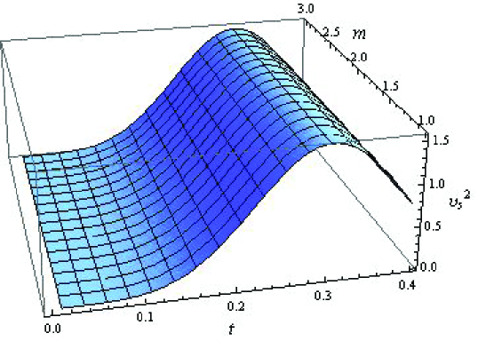
Figure 7: Plot of squared speed of sound parameter for $\alpha=22.05$, $\rho_{m_{0}}=0.23$, $a_{0}=1$, $d_{1}=0.3$, $\Omega_{m_{0}}=0.313$ and $H_{0}=67.48$.

The $\omega_{eff}-\omega^{\prime}_{eff}$ plane can be found by using Eq.(26) as follows

$$\omega^{\prime}_{eff} = \frac{-2d_{1}}{\alpha mt}(1+\frac{\rho_{m_{0}}t^{1-3m+3d_{1}}}{\alpha ma_{0}^{3}}+\frac{3md_{1}}{1-3m+3md_{1}})^{-1}-\frac{1}{\alpha m^{2}a_{0}^{3}}[(\frac{-3m+1}{3m}-d_{1}$$

$$\times (\frac{-2}{\alpha t}+\frac{-3m+1}{3m}+2))\rho_{m_{0}}t^{1-3m+3d_{1}}(1-3m+3d_{1})](1+\frac{\rho_{m_{0}}t^{1-3m+3d_{1}}}{\alpha ma_{0}^{3}}$$

$$+ \frac{3md_{1}}{1-3m+3md_{1}})^{-2}.$$

Figure 8 represents the $\omega_{eff}-\omega^{\prime}_{eff}$ plane for GDE $f(G)$ model with three distinct values of $m$, i.e., $m=2,2.4$ and $2.8$. It is found that $\omega_{eff}-\omega^{\prime}_{eff}$ plane corresponds to freezing region for all considered values of $m$ showing a consistent behavior with our current accelerated expanding universe.

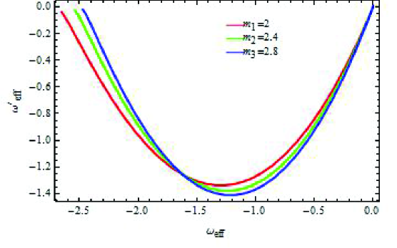
Figure 8: Trajectories of $\omega_{eff}-\omega^{\prime}_{eff}$ for GDE $f(G)$ model with $\alpha=22.05$, $\rho_{m_{0}}=0.23$, $a_{0}=1$, $d_{1}=0.3$, $\Omega_{m_{0}}=0.313$ and $H_{0}=67.48$.

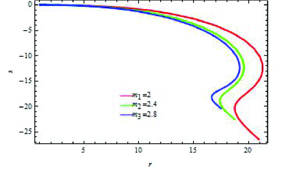
Figure 9: Trajectories of $r-s$ for GDE $f(G)$ model using $\alpha=22.05$, $\rho_{m_{0}}=0.23$, $a_{0}=1$, $d_{1}=0.3$, $\Omega_{m_{0}}=0.313$ and $H_{0}=67.48$.

The corresponding $r-s$ plane is given by

$$r = 2[\frac{1}{2}+\frac{3}{2}((\frac{-3m+1}{3m}-d_{1}(\frac{-2}{\alpha t}+\frac{-3m+1}{3m}+2))(1+\frac{\rho_{m_{0}}t^{1-3m+3d_{1}}}{\alpha ma_{0}^{3}}$$

$$+ \frac{3md_{1}}{1-3m+3md_{1}})^{-1})]^{2}+\frac{1}{2}+\frac{3}{2}((\frac{-3m+1}{3m}-d_{1}(\frac{-2}{\alpha t}+\frac{-3m+1}{3m}+2))$$

$$\times (1+\frac{\rho_{m_{0}}t^{1-3m+3d_{1}}}{\alpha ma_{0}^{3}}+\frac{3md_{1}}{1-3m+3md_{1}})^{-1})+\frac{3d_{1}}{\alpha t^{2}}(1+\frac{\rho_{m_{0}}t^{1-3m+3d_{1}}}{\alpha ma_{0}^{3}}$$

$$+ \frac{3md_{1}}{1-3m+3md_{1}})^{-1}+\frac{3\rho_{m_{0}}t^{1-3m+3d_{1}}(1-3m+3d_{1})}{2\alpha ma_{0}^{3}t}((\frac{-3m+1}{3m}-d_{1}$$

$$\times (\frac{-2}{\alpha t}+\frac{-3m+1}{3m}+2))(1+\frac{\rho_{m_{0}}t^{1-3m+3d_{1}}}{\alpha ma_{0}^{3}}+\frac{3md_{1}}{1-3m+3md_{1}})^{-2}).$$

$$s = \frac{1}{2}((\frac{-3m+1}{3m}-d_{1}(\frac{-2}{\alpha t}+\frac{-3m+1}{3m}+2))(1+\frac{\rho_{m_{0}}t^{1-3m+3d_{1}}}{\alpha ma_{0}^{3}}$$

$$+ \frac{3md_{1}}{1-3m+3md_{1}})^{-1})(2[\frac{1}{2}+\frac{3}{2}((\frac{-3m+1}{3m}-d_{1}(\frac{-2}{\alpha t}+\frac{-3m+1}{3m}+2))$$

$$\times (1+\frac{\rho_{m_{0}}t^{1-3m+3d_{1}}}{\alpha ma_{0}^{3}}+\frac{3md_{1}}{1-3m+3md_{1}})^{-1})]^{2}-\frac{1}{2}+\frac{3}{2}((\frac{-3m+1}{3m}$$

$$- d_{1}(\frac{-2}{\alpha t}+\frac{-3m+1}{3m}+2))(1+\frac{\rho_{m_{0}}t^{1-3m+3d_{1}}}{\alpha ma_{0}^{3}}+\frac{3md_{1}}{1-3m+3md_{1}})^{-1})$$

$$+ \frac{3d_{1}}{\alpha t^{2}}(1+\frac{\rho_{m_{0}}t^{1-3m+3d_{1}}}{\alpha ma_{0}^{3}}+\frac{3md_{1}}{1-3m+3md_{1}})^{-1}+\frac{3\rho_{m_{0}}t^{1-3m+3d_{1}}}{2\alpha ma_{0}^{3}t}$$

$$\times (1-3m+3d_{1})((\frac{-3m+1}{3m}-d_{1}(\frac{-2}{\alpha t}+\frac{-3m+1}{3m}+2))(1+\frac{\rho_{m_{0}}t^{1-3m+3d_{1}}}{\alpha ma_{0}^{3}}$$

$$+ \frac{3md_{1}}{1-3m+3md_{1}})^{-2})).$$

The trajectories of $r-s$ plane for GDE $f(G)$ model with $m=2,2.4$ and $2.8$ are shown in Figure 9. These plots show that the $r-s$ plane leads to the Chaplygin gas model regimes for all three values of $m$.

5 Concluding Remarks

In this paper, we have used reconstruction scheme of GDE $f(G)$ model for both interacting as well as non-interacting scenario with power-law form of the scale factor. We have established a correspondence of GDE with $f(G)$ gravity and reconstructed $f(G)$ model by assuming GDE parameter $\alpha=22.05$. To examine cosmological behavior of the reconstructed $f(G)$ model, we have discussed the cosmological parameters as well as phase planes. The final results are summarized as follows.

• The reconstructed GDE $f(G)$ model (Figure 1) represents decreasing behavior initially and then it attains increasing behavior forever. This shows that the reconstructed model is a realistic one.

• The EoS parameter (Figure 2) shows quintessence era of the universe for non-interacting case whereas it represents phantom phase (Figure 6) in interacting scenario. Hence, our results are consistence with the current accelerated cosmic behavior. We can conclude that the GDE $f(G)$ model favors the DE phenomenon.

• The squared speed of sound parameter for both interacting (Figures 3) and non-interacting (7) cases indicates stability of the reconstructed model for current as well as later epoch of time in the interval $1<m<3$ respectively.

• The evolutionary behavior of the $\omega_{DE}-\omega^{\prime}_{DE}$ plane (Figures 4 and 8) for $m=2,2.4$ and $2.8$ provides the thawing region for non-interacting case whereas freezing region for interacting scenario, respectively. Hence, cosmological expansion is more accelerating in interacting case as compared with non-interacting scenario.

• The corresponding trajectories of $r-s$ plane indicate Chaplygin gas model for all three values of $m$ in both cases. Furthermore, it attains CDM limit but $\Lambda$CDM limit cannot be achieved.

We have found that the GDE $f(G)$ model indicates stable behavior and is consistent with the current behavior of the universe depending on the appropriate choice of ghost parameter. Chattopadhyay [19] established the correspondence of $f(T)$ theory with GDE model and found that the EoS parameter never crosses the phantom divide line in non-interacting scenario. Our results are consistent with these outcomes. Saaidi et al. [16] discussed the correspondence between $f(R)$ theory and GDE model and found that the reconstructed model is stable while the EoS parameter passes through the phantom divide line for interacting case. Our results are also consistent with these consequences. Finally, if we take the coupling constant $d_{1}=0$ then all results of interaction reduce to non-interacting scheme.

References

- [1] Sahni, V. and Starobinsky, A.A.: Int. J. Mod. Phys. D 9(2000)373; Peebles, P.J.E. and Ratra, B.: Rev. Mod. Phys. 75(2003)559.
- [2] Bagla, J.S., Jassal, H.K. and Padmanabhan, T.: Phys. Rev. D 67(2003)063504; Caldwell, R.: Phys. Lett. B 545(2002)23; Zhang, X., Zhang, J. and Wu, F.Q.: J. Cosmol. Astropart. Phys. 607(2005)35; Cai, R.G.: Phys. Lett. B 657(2007)228.
- [3] Linder, E.V.: Phys. Rev. D 81(2010)127301; Sharif, M. and Rani, S.: Astrophys. Space Sci. 346(2013)573.
- [4] Witten, E.: Nucl. Phys. B 156(1979)269; Veneziano, G.: Nucl. Phys. B 159(1979)213.
- [5] Kawarabayashi, K. and Ohta, N.: Nucl. Phys. B 175(1980)477; Nath, P. and Arnowitt, R.L.: Phys. Rev. D 23(1981)473.
- [6] Bjorken, J.D.: arXiv:astro-ph/0404233; Klinkhamer, F.R. and Volovik, E.G.: Phys. Rev. D 77(2008)085015; ibid. 78(2008)063528; ibid. 79(2009)063527.
- [7] Nojiri, S. and Odintsov, S.D.: Phys. Lett. B 631(2005)1.
- [8] Cognola, G. et al.: Phys. Rev. D 73(2006)084007.
- [9] Nojiri, S., Odintsov, S.D. and Gorbunova, O.G.: J. Phys. A 39(2006)6627.
- [10] De Felice, A. and Tsujikawa, S.: Phys. Rev. D 80(2009)063516.
- [11] Setare, M.R. and Saridakis, E.N.: Phys. Lett. B 670(2008)1.
- [12] Setare, M.R. and Saridakis, E.N.: Phys. Lett. B 668(2008)177.
- [13] Setare, M.R.: Int. J. Mod. Phys. 17(2008)2219; Setare, M.R., Momeni, D. and Moayedi, S.K.: Astrophys. Space Sci. 338(2012)405.
- [14] Sheykhi, A. and Movahed, M.S.: Gen. Relativ. Gravit. 44(2012)449.
- [15] Sadeghi, J. et al.: J. Cosmol. Astropart. Phys. 12(2013)031.
- [16] Saaidi, K. et al.: Int. J. Mod. Phys. D 21(2012)1250057.
- [17] Alavirad, H. and Sheykhi, A.: Phys. Lett. B 734(2014)148.
- [18] Fayaz, V. et al.: Can. J. Phys. 92(2014)168.
- [19] Chattopadhyay, S.: Eur. Phys. J. Plus 129(2014)82.
- [20] Fayaz, V. et al.: Eur. Phys. J. Plus 131(2016)22.
- [21] Zhou, S., Copeland, E.J. and Saffin, P.M.: J. Cosmol. Astropart. Phys. 07(2009)009.
- [22] Sheykhi, A. and Bagheri, A.: Europhys. Lett. 95(2011)39001.
- [23] Chattopadhyay, S.: Astrophys. Space Sci. 352(2014)937.
- [24] Shamir, F.M.: J. Exp. Theor. Phys. 123(2016)607.
- [25] Houndjo, M. et al.: Can. J. Phys. 92(2014)1528
- [26] Urban, F.R. and Zhitnitsky, A.R.: Phys. Rev. D 80(2009)063001; Rozas-Fernández, A.: Phys. Lett. B 709(2012)313.
- [27] Caldwell, R. and Linder, E.V.: Phys. Rev. Lett. 95(2005)141301.
- [28] Sahni, V. et al.: J. Exp. Theor. Phys. Lett. 77(2003)201.
- [29] Cai, R.G. and Su, Q.: Phys. Rev. D 81(2010)103514.
- [30] Sun, C.Y. and Yue, R.H.: Phys. Rev. D 85(2012)043010.