Regular Bouncing Solutions, Energy Conditions
and the Brans-Dicke Theory

Abstract

In general, to avoid a singularity in cosmological models involves the introduction of exotic kind of matter fields, for example, a scalar field with negative energy density. In order to have a bouncing solution in classical General Relativity, violation of the energy conditions is required. In this work, we discuss a case of the bouncing solution in the Brans-Dicke theory with radiative fluid that obeys the energy conditions, and with no ghosts.

1 Introduction

One of the main drawbacks of the standard cosmological model is the existence of an initial singularity. Singularities are a common feature in different applications of General Relativity (GR) when matter fields obey reasonable energy conditions, called normal fields. Hence, the avoidance of a singularity generally implies the introduction of exotic matter fields, such as phantom fields (i.e., a scalar field with negative energy density). However, there are situations where normal fields may also lead to the avoidance of singularities if some non-trivial coupling is introduced. This implies that the matter sector must contain more than one component which interacts directly among themselves. Many non-singular solutions in non-minimal coupled theories are also obtained due to the presence of fields which appear phantom when the theory is formulated in terms of a minimally-coupled system.

The purpose of this note is to call attention to a non-singular model with fluids that obey the energy conditions and with no ghosts is possible even in the most simple scalar-tensor theory, the Brans-Dicke theory. We will essentially analyse the solutions determined by Gurevich et al [1] for a flat homogeneous and isotropic universe. Our goal is to identify some properties of these already known solutions which, to our knowledge, have not been studied in some of their aspects . These properties may be relevant for the construction of a coherent and realistic cosmological model, in particular for solving the singularity problem.

The Brans-Dicke theory of gravitation is one of the most important alternative theories to GR, where the inverse of the gravitational constant $G$ is replaced by a scalar filed $\phi$, which can vary in space and time. It was developed by C. Brans and R.H. Dicke [5] in order to implement the Mach’s principle in a relativistic theory. The theory has received recently much attention of the scientific community [6]-[12].

The paper is organized as follows. In section 2 we describe the system, its equation of motion, and review the solutions for the radiative case studied by Gurevich et al. In section 3 we analyze the bouncing properties of the solutions. In section 4 we discuss the energy conditions, and develop the perturbation over specific background. In section 5 we give our final remarks.

2 The classical equations of motion and Gurevich et al Solutions

The Brans-Dicke theory is defined by the action

$${\cal A}=\frac{1}{16\pi}\int d^{4}x\biggr{\{}\sqrt{-g}\biggr{(}\phi R-\frac{\omega}{\phi}\left(\nabla\phi\right)^{2}\biggl{)}+{\cal L}_{m}\biggl{\}},$$ (1)

where $\phi$ is a scalar field, ${\cal L}_{m}$ is the matter Lagrangian and $\omega$ is a free parameter. This is the prototype of a scalar-tensor theory where the non-minimal coupling occurs between the gravitational term and the scalar field. The main goal of the Brans-Dicke theory was to introduce a varying gravitational coupling through the scalar field $\phi$. It can been seen as the first example of Galileons and Horndesky-type theories [13].

Local tests limit the value of the parameter $\omega$ to be very large [14], what in principle renders the theory essentially equivalent to GR. However, extensions of the Brans-Dicke theory leave place for a varying coupling parameter $\omega$. The Horndesky class of theories cover all possibilities without Ostrogradsky instabilities including the Brans-Dicke theory in its traditional form. This opens the possibility for small values of the coupling parameter in the past (which can be even negative), evolving to a huge value today. Also, the low energy effective action of string theory leads to Brans-Dicke theory with $\omega=-1$ [15]. Brane configurations may allow even more negative values of $\omega$. In evoking this connection, we have mainly in mind the domain of application of the string effective theory which is the primordial universe.

The Brans-Dicke theory field equations read

$$R_{\mu\nu}-\frac{1}{2}g_{\mu\nu}R = \frac{8\pi}{\phi}T_{\mu\nu}+\frac{\omega}{\phi^{2}}\biggr{(}\nabla_{\mu}\phi\nabla_{\nu}\phi-\frac{1}{2}g_{\mu\nu}\nabla_{\alpha}\phi\nabla^{\alpha}\phi\biggl{)}$$ (2)

$$+ \frac{1}{\phi}(\nabla_{\mu}\nabla_{\nu}\phi-g_{\mu\nu}\Box\phi),$$

$$\Box\phi = \frac{8\pi}{3+2\omega}T,$$ (3)

$$\nabla_{\mu}T^{\mu\nu} = 0,$$ (4)

where $w$ is a constant. For a flat FLRW metric

$$ds^{2}=dt^{2}-a(t)^{2}(dx^{2}+dy^{2}+dz^{2}),$$ (5)

the field equations reduce to

$$3\biggr{(}\frac{\dot{a}}{a}\biggl{)}^{2} = 8\pi\frac{\rho}{\phi}+\frac{\omega}{2}\biggl{(}\frac{\dot{\phi}}{\phi}\biggl{)}^{2}-3\frac{\dot{a}}{a}\frac{\dot{\phi}}{\phi},$$ (6)

$$2\frac{\ddot{a}}{a}+\biggr{(}\frac{\dot{a}}{a}\biggl{)}^{2} = -8\pi\frac{p}{\phi}-\frac{\omega}{2}\biggl{(}\frac{\dot{\phi}}{\phi}\biggl{)}^{2}-\frac{\ddot{\phi}}{\phi}-2\frac{\dot{a}}{a}\frac{\dot{\phi}}{\phi},$$ (7)

$$\ddot{\phi}+3\frac{\dot{a}}{a}\dot{\phi} = \frac{8\pi}{3+2\omega}(\rho-3p),$$ (8)

$$\dot{\rho}+3\frac{\dot{a}}{a}(\rho+p) = 0.$$ (9)

Gurevich et al [1] determined the general solution for the cosmological isotropic and homogeneous flat universe with a perfect fluid with an equation of state $p=\alpha\rho$, where $\alpha$ is a constant such that $0\leq\alpha\leq 1$. The general solution for $\omega>-\frac{3}{2}$ (a case where the energy conditions for the scalar field are satisfied) reads

$$a(\theta) = a_{0}(\theta-\theta_{+})^{r_{+}}(\theta-\theta_{-})^{r_{-}},$$ (10)

$$\phi(\theta) = \phi_{0}(\theta-\theta_{+})^{s_{+}}(\theta-\theta_{-})^{s_{-}},$$ (11)

with the definitions,

$$r_{+} = \frac{\omega}{3\biggl{[}\sigma\mp\sqrt{1+\frac{2}{3}\omega}\biggr{]}},\quad r_{-}=\frac{\omega}{3\biggl{[}\sigma\pm\sqrt{1+\frac{2}{3}\omega}\biggr{]}},$$ (12)

$$s_{+} = \frac{1\mp\sqrt{1+\frac{2}{3}\omega}}{\sigma\mp\sqrt{1+\frac{2}{3}\omega}},\quad s_{-}=\frac{1\pm\sqrt{1+\frac{2}{3}\omega}}{\sigma\pm\sqrt{1+\frac{2}{3}\omega}},$$ (13)

where $\sigma=1+\omega(1-\alpha)$, and $a_{0},\phi_{0},\theta_{\pm}$ are arbitrary constants, with $\theta_{+}>\theta_{-}$. The time coordinate $\theta$ is connected with the cosmic time $t$ by

$$dt=a^{3\alpha}d\theta.$$ (14)

For $\omega<-\frac{3}{2}$, where there is violation of the energy conditions for the scalar field in the Einstein frame, as it will be discussed below, the solutions read

$$a =a_{0}\Big{[}\left(\theta+\theta_{-}\right)^{2}+\theta_{+}^{2}\Big{]}^{\big{(}1+(1-\alpha)\omega\big{)}/{A}}e^{\pm 2f(\theta)/A}\ ,$$ (15)

$$\phi =\phi_{0}\left[\left(\theta+\theta_{-}\right)^{2}+\theta_{+}^{2}\right]^{{(1-3\alpha)}/{A}}e^{\pm 6\left(1-\alpha\right)f(\theta)/A}\ ,$$ (16)

where

$$f(\theta) =\sqrt{\frac{2|\omega|-3}{3}}\arctan\left(\frac{\theta+\theta_{-}}{\theta_{+}}\right)$$ (17)

$$A =2\left(2-3\alpha\right)+3\omega\left(1-\alpha\right)^{2}$$ (18)

In the case $\omega>-\frac{3}{2}$, the condition to have a regular bounce can be expressed by requiring $r_{+}<0$ (the scale factor is infinite at one asymptote), $r_{+}+r_{-}>0$ (the scale factor is infinite at another asymptote) and $3\alpha r_{+}+1<0$ (the cosmic time varies from $-\infty$ to $+\infty$). These conditions imply that a regular bounce may be obtained for $\frac{1}{4}<\alpha<1$ and $-\frac{3}{2}<\omega\leq-\frac{4}{3}$. The case $\alpha=1$ is quite peculiar, and contains no bounce [7].

We will be interested here mainly in a scenario for the early universe. Thus, we will consider in detail the radiative universe. The Gurevich et al solution for the radiative case ($p=\frac{1}{3}\rho$) is given by the following expressions

• $\omega>-\frac{3}{2}$:

  $$a(\eta) = a_{0}(\eta-\eta_{+})^{\frac{1}{2}(1\pm r)}(\eta-\eta_{-})^{\frac{1}{2}(1\mp r)},$$ (19)

  $$\phi(\eta) = \phi_{0}(\eta-\eta_{+})^{\mp r}(\eta-\eta_{-})^{\pm r};$$ (20)

• $\omega<-\frac{3}{2}$:

  $$a(\eta) = a_{0}[(\eta+\eta_{-})^{2}+\eta_{+}^{2}]^{\frac{1}{2}}e^{\pm\frac{1}{\sqrt{\frac{2}{3}|\omega|-1}}\arctan\frac{\eta+\eta_{-}}{\eta_{+}}},$$ (21)

  $$\phi(\eta) = \phi_{0}e^{\mp\frac{2}{\sqrt{\frac{2}{3}|\omega|-1}}\arctan\frac{\eta+\eta_{-}}{\eta_{+}}}.$$ (22)

In these expressions,

$$r=\frac{1}{\sqrt{1+\frac{2}{3}\omega}},$$ (23)

$\eta$ is the conformal time and $\eta_{\pm}$ are constants such that $\eta_{+}>\eta_{-}$.

If we perform a conformal transformation of the Brans-Dicke action such that $g_{\mu\nu}=\phi^{-1}\tilde{g}_{\mu\nu}$, we re-express it in the so-called Einstein’s frame

$${\cal A}=\frac{1}{16\pi}\int d^{4}x\biggr{\{}\sqrt{-\tilde{g}}\biggr{[}\tilde{R}-\biggr{(}\omega+\frac{3}{2}\biggl{)}\frac{\left(\nabla\phi\right)^{2}}{\phi^{2}}\biggl{]}+{\cal L}_{m}\biggl{\}}.$$ (24)

Thus, in the Einstein frame, $\omega>-\frac{3}{2}$ corresponds to an ordinary scalar field with positive energy density, while for $\omega<-\frac{3}{2}$, the kinetic term of the scalar field changes sign, and it becomes a phantom field with negative energy density. Remember that the radiative fluid is conformal invariant.

3 Analysis of the Solutions

For $\omega\geq 0$ the scale factor displays an initial singularity followed by expansion, reaching $a\rightarrow\infty$ as $\eta\rightarrow\infty$. Note that the radiative universe of GR characterised by

$$a\propto\eta,$$ (25)

can be recovered from the above solutions if $\eta_{\pm}=0$, in the limit $\omega\rightarrow\infty$ when $\eta_{+}=\eta_{-}$, or in the asymptotic limit $\eta\rightarrow\infty$.

The GR behaviour of the scale factor is also achieved for $\omega=0$. However, in this case, the scalar field (the inverse of the gravitational coupling) varies with time, and its variation depends essentially on the sign in the exponent in Eqs. (19)(20). For the upper sign, we find

$$a(\eta) = a_{0}(\eta-\eta_{+}),$$ (26)

$$\phi(\eta) = \phi_{0}\frac{\eta-\eta_{-}}{\eta-\eta_{+}},$$ (27)

and the scalar field decreases monotonically from infinite to a constant (positive) value as the universe evolves. For the lower sign, the behaviour of the functions are given by

$$a(\eta) = a_{0}(\eta-\eta_{-}),$$ (28)

$$\phi(\eta) = \phi_{0}\frac{\eta-\eta_{+}}{\eta-\eta_{-}},$$ (29)

and the scalar field increases monotonically from an infinite negative value to a constant positive value as the universe evolves: initially there is a repulsive gravitational phase. This can be considered as a Big Rip type singularity since it occurs when $a\rightarrow\infty$ at finite proper time.

Bounce solutions can be obtained from the Gurevich et al solutions in the radiative case if the lower sign is chosen in Eqs. (19)(20) for $-\frac{3}{2}<\omega<0$. However, there is a singularity at $\eta=\eta_{+}$ for $-\frac{4}{3}<\omega<0$ at $\eta=\eta_{+}$, even if the scale factor diverges at this point. On the other hand, if $-\frac{3}{2}<\omega\leq-\frac{4}{3}$, the bounce solutions are always regular, with no curvature singularity. In this last case, there are two possible scenarios (thanks to time reversal invariance):

1. A universe that begins at $\eta=\eta_{+}$ with $a\rightarrow\infty$, with an infinite value for the gravitational coupling ($\phi=0$), evolving to the other asymptotic limit with $a\rightarrow\infty$ but with $\phi$ constant and finite;

2. The reversal behaviour occurs for $-\infty<\eta<-\eta_{+}$.

In both cases, the cosmic times ranges $-\infty<t<\infty$. The dual solution in the Einstein frame for $-\frac{3}{2}<\omega\leq-\frac{4}{3}$ is given by $b(\eta)=b_{0}(\eta-\eta_{+})^{1/2}(\eta-\eta_{-})^{1/2}$ (with $b=\phi^{1/2}a$) and contains an initial singularity. This can be considered as a specific case of ”conformal continuation” in the scalar-tensor gravity proposed in [16].

For the special case $\omega=-\frac{4}{3}$ there is still no singularity if we choose the lower sign. In this case, the scale factor and the scalar field behaves

$$a(\eta)\propto\frac{(\eta-\eta_{-})^{2}}{\eta-\eta_{+}},\quad\phi(\eta)\propto\biggr{(}\frac{\eta-\eta_{+}}{\eta-\eta_{-}}\biggl{)}^{3}.$$ (30)

If $-\infty<\eta<\eta_{+}$ the universe begins with $a\rightarrow\infty$, with $\phi$ constant and finite, while in the remote future $a\rightarrow\infty$ and $\phi=0$. If we choose the interval $\eta_{+}\leq\eta<\infty$, the scenario is reversed, and we get the possibility to have a constant gravitational coupling today.

For $\omega=-\frac{4}{3}$ and the upper sign the solutions exhibit an initial singularity:

$$a(\eta) \propto \frac{(\eta-\eta_{+})^{2}}{\eta-\eta_{-}},$$ (31)

$$\phi(\eta) \propto \biggr{(}\frac{\eta-\eta_{-}}{\eta-\eta_{+}}\biggl{)}^{3}.$$ (32)

Similar features for the scale factor and the scalar field are reproduced for $\omega<-\frac{3}{2}$. However the scalar field has a phantom behaviour as already stated.

4 Energy Conditions and Perturbations

An important aspect of these solutions concerns the energy conditions. In general in order to have a bouncing solution, violation of the energy conditions is required. The strong and null energy conditions in General Relativity are given by

$$\frac{\ddot{a}}{a} = -\frac{4\pi G}{3}(\rho+3p)>0,$$ (33)

$$-2\frac{\ddot{a}}{a}+2\biggr{(}\frac{\dot{a}}{a}\biggl{)} = 8\pi G(\rho+p)>0.$$ (34)

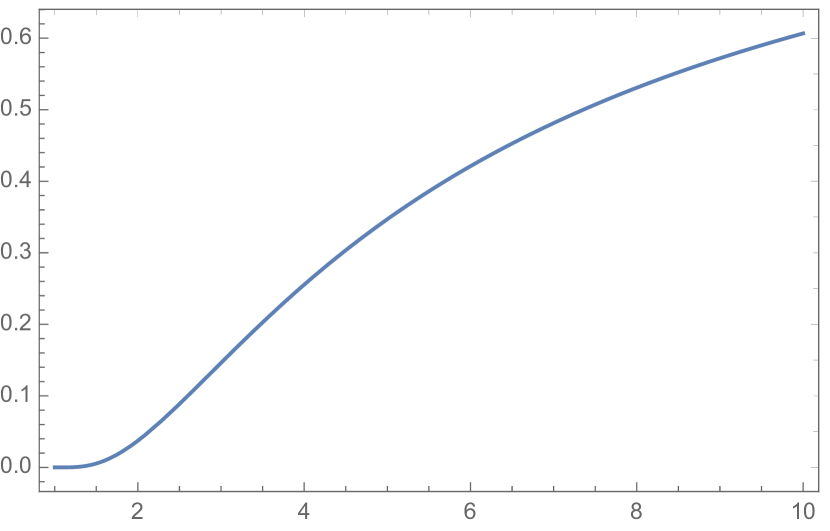
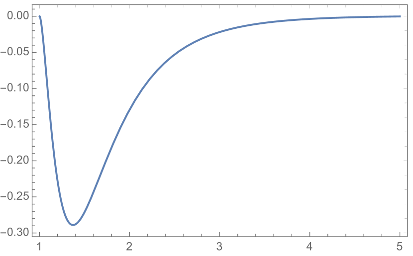
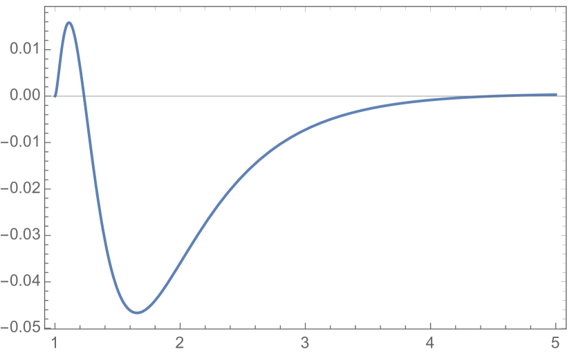
Figure 1: Behaviour of the scale factor (left), the scalar field (center left), of the ”effective” strong energy condition (center right) and ”effective” null energy condition (right) for $\omega=-1.43$ lower sign.

In order to use the energy condition in this form the Brans-Dicke theory must be reformulated in the Einstein frame. It is easy to verify that both energy conditions are satisfied as far as $\omega<-\frac{3}{2}$. This is consistent with the fact that in the Einstein frame the cosmological scenarios are singular unless $\omega<-\frac{3}{2}$. On the other hand, in the original Jordan frame there are non singular models if $-\frac{3}{2}<\omega<-\frac{4}{3}$. But in this range the scalar field obeys the energy condition. The effects leading to the avoidance of the singularity come from the non-minimal coupling. We plot the ”effective” energy condition, represented in the left-hand side of Eqs. (33)(34), taking into account the effects of the non-minimal coupling. If we consider only the left-hand side of the relations Eqs. (33)(34), the effects of the interaction due to the non-minimal coupling are included, and the energy conditions can be violated even if the matter terms do not violated them. In Fig. 1 we show the expressions for these relations for some values of $\omega$.

It is interesting to notice that, for the most usual fluids employed in cosmology, the case of the radiative fluid is the only one where the possibility of obtaining a singularity-free scenario preserving the energy conditions is possible, at least in the Brans-Dicke theory . For a matter fluid ($p=0$), the scale factor can be expressed in terms of the cosmic time and behaves, according the Gurevich et al solution, as

$$a(t)=a_{0}(t-t_{+})^{r_{\pm}}(t-t_{-})^{r_{\mp}},\quad r_{\pm}=\frac{1+\omega\pm\sqrt{1+\frac{2}{3}\omega}}{4+3\omega},$$ (35)

$t_{\pm}$ being integration constants such that $t_{+}>t_{-}$. There is a singular bounce for negative values of $\omega$ . In their work, Gurevich et al does not display explicitly the solution for a vacuum equation of state ($p=-\rho$) but it can be deduced from a general expression they write down. For $p=-\rho$ the general solution reduces to

$$a(\theta) = a_{0}(\theta-\theta_{+})^{s_{\pm}}(\theta-\theta_{-})^{s_{\mp}},\quad$$ (36)

$$s_{\pm}=\frac{1+2\omega\pm\sqrt{1+\frac{2}{3}\omega}}{2(5+6\omega)},$$ (37)

where $\theta$ is a parametric time, which is connected to cosmic time through the relation $dt=a^{-3}d\theta$. As in the pressureless matter case, bounce solutions exist for negative $\omega$, but they are singular. Of course, in both pressureless and cosmological constant cases singularity free solutions are possible if $\omega<-\frac{3}{2}$ but this implies a phantom scalar field.

Now, let us turn to perturbations. Using the synchronous coordinate condition and particularising the expressions for a radiative fluid, the perturbed equations read

$$\ddot{h}+2H\dot{h} = \frac{16\pi}{\phi}(\delta-\lambda)+2\ddot{\lambda}+4\frac{\dot{\phi}}{\phi}(1+\omega)\dot{\lambda},$$ (38)

$$\ddot{\lambda}+\biggr{(}3H+2\frac{\dot{\phi}}{\phi}\biggl{)}\dot{\lambda}+\frac{k^{2}}{a^{2}}\lambda = \frac{\dot{\phi}}{\phi}\frac{\dot{h}}{2},$$ (39)

$$\dot{\delta}+\frac{4}{3}\biggr{(}\theta-\frac{\dot{h}}{2}\biggl{)} = 0,$$ (40)

$$\dot{\theta}+H\theta = \frac{k^{2}}{4a^{2}}\delta.$$ (41)

In these expressions we have

$$h=\frac{k_{kk}}{a^{2}},\quad\delta=\frac{\delta\rho}{\rho},\quad\lambda=\frac{\delta\phi}{\phi},\quad\theta=\partial_{i}\delta u^{i}.$$ (42)

Moreover, $k$ is the wavenumber coming from the Fourier decomposition and $H$ is the Hubble function.

The evolution of scalar perturbations in the Brans-Dicke theory has been studied in Ref. [18], and some features connected with the Gurevich et al solutions have been displayed in Ref. [19]. For the bouncing regular solutions analysed here, it is natural to implement the Bunch-Davies vacuum state as the initial condition. However, it is known that in bounce scenario a flat or almost flat spectrum requires a matter dominant period in the contraction phase. This is not obviously the case for the regular Gurevich et al solutions which is verified for a radiative fluid.

In Fig. 2 we display the evolution for the density contrast for $k=0.01$ and $k=0.1$ (in the units of the current Hubble scale), as well as the dependence of the spectral index $n_{s}$ as a function of the wavenumber $k$. The spectral index is defined as usual

$$\Delta=k^{3}\delta_{k}^{2}=k^{n_{s}-1}.$$ (43)

We display the evolution of the perturbations and the dimensionless power spectrum which exhibits a clear disagreement with the observations (compare with similar results obtained in Ref. [20]). Since the model studied here requires a single radiative fluid such somehow negative result could be expected from the beginning.

5 Discussion

In this paper we have shown that regular bounce solutions without any phantom field, even in the Einstein frame, can arise in Brans-Dicke theories containing fluids obeying the equation of state $p=\alpha\rho$ if $\frac{1}{4}\leq\alpha<1$, and a Brans-Dicke parameter $\omega$ lying in the interval $-\frac{3}{2}\leq\omega\leq-\frac{4}{3}$, enlarging the parameter space in which such cosmological models can emerge in this class of theories.

We analysed in detail the radiative case with $\alpha=\frac{1}{3}$. A bounce can be obtained if we choose the lower sign in Eqs. (19)(20) for $-\frac{3}{2}<\omega<0.$ Moreover, for $-\frac{3}{2}<\omega\leq\frac{4}{3}$ the bounce is regular with no curvature singularity, but for $-\frac{4}{3}<\omega<0$ there is a singularity at $\eta=\eta_{+}$, even if the scale factor diverges at this point. In the case of $\omega=-\frac{4}{3}$ there is still no singularity if we choose the lower sign, and there is an initial singularity for the upper sign. The solutions Eqs. (21)(22) with $\omega<-\frac{3}{2}$ have a similar behaviour, but with a phantom field in the Einstein frame.

It is generally expected that the violation of the energy conditions is required in order to have classical bounce solutions, even in the non-minimal coupling case: in this situation, phantom fields would appear in the Einstein frame. We discussed this point in detail for the case of the radiative fluid in the Brans-Dicke theory (with a flat spatial section), where we have shown that it is possible to obtain non-singular solutions preserving the energy conditions even in the Einstein frame, and we have shown that this property holds for any Brans-Dicke theory in which $\frac{1}{4}\leq\alpha<1$, and $-\frac{3}{2}\leq\omega\leq-\frac{4}{3}$. This generalization allows the possibility of constructing more involved and realistic regular bouncing solutions, in which the power spectrum of cosmological perturbations could be in accordance with present observations. This is one of our goals of our future investigations in this subject.

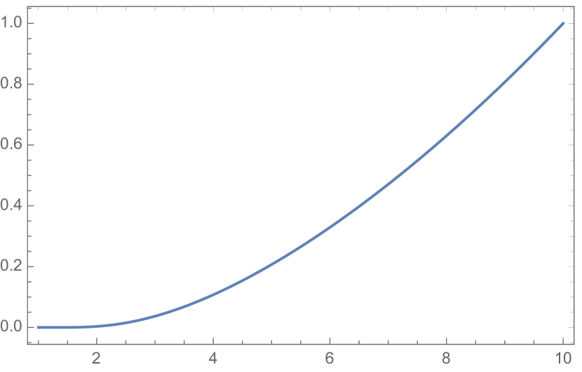
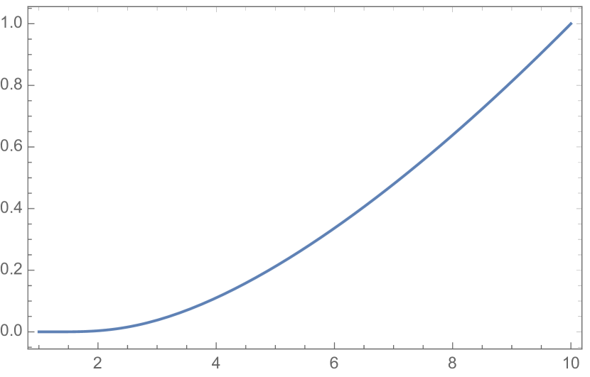
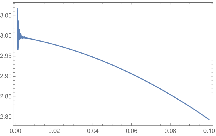
Figure 2: The behaviour of the density contrast is displayed for $k=0.01$ (left panel) and for $k=0.1$ (center panel). The normalization has been chosen such that the final density contrast is equal to one. In the right panel is shown the dependence of the spectral index $n_{s}$ on the wavenumber $k$. All the figures were obtained for $\omega=-1.43$ lower sign.

References

- [1] L. E. Gurevich, A. M. Finkelstein, V. A. Ruban, Astrophys. Spc. Sci. 22, 231 (1973).
- [2] J. D. Barrow, P. Parsons, Phys.Rev. D 55, 1906-1936 (1997).
- [3] T. Clifton, J. D. Barrow, Phys. Rev. D 73, 104022 (2006).
- [4] J. P. Mimoso, D. Wands, Phys. Rev. D 52, 5612 (1995).
- [5] C. Brans, R. H. Dicke, Phys. Rev. 124, 925-935 (1961).
- [6] M. Rossi, M. Ballardini, M. Braglia, F. Finelli, D. Paoletti, A. A. Starobinsky, C. Umiltà, arXiv:1906.10218 [astro-ph] (2019).
- [7] G. Brando, J. C. Fabris, F. T. Falciano, O. Galkina, arXiv:1810.07860 [gr-qc] (2018).
- [8] G. Brando, F. T. Falciano, L. F. Guimarães, Phys. Rev. D 98, 044027 (2018).
- [9] A. Paliathanasis, M. Tsamparlis, S. Basilakos, John D. Barrow, Phys.Rev. D 93 (2016).
- [10] D. A. Tretyakova, B. N. Latosh and S. O. Alexeyev, Class. Quantum Grav. 32, 185002 (2015).
- [11] V. Faraoni, J. Côté , A. Giusti, arXiv:1906.05957 [gr-qc] (2019).
- [12] E. Frion and C. R. Almeida, Phys. Rev. D 99,023524 (2019).
- [13] T. Kobayashi, Rept. Prog. Phys. 82, 086901 (2019).
- [14] C. M. Will, Theory and experiment in gravitational physics, 2 ed., Cambridge University Press, (2018).
- [15] M. J. Duff, Ramzi R. Khuri, J. X. Lu, Phys.Rept. 259, 213-326 (1995).
- [16] K. A. Bronnikov, J. Math. Phys. 43, 6096-6115 (2002).
- [17] A. A. Starobinsky, Sov. Astron. Lett. 7, 36-38 (1981).
- [18] J. P. Baptista, J. C. Fabris and S.V.B. Gonçalves, Astrophys.Space Sci. 246, 315 (1996).
- [19] A. B. Batista, J. C. Fabris and J. P. Baptista, Comptes R. Acad. Scie. 309, 791 (1989).
- [20] Sandro D. P. Vitenti and Nelson Pinto-Neto, Phys. Rev. D 85, 023524 (2012).