Free surface of a liquid in a rotating frame with time-depend velocity

Abstract

The shape of liquid surface in a rotating frame depends on the angular velocity. In this experiment, a fluid in a rectangular container with a small width is placed on a rotating table. A smartphone fixed to the rotating frame simultaneously records the fluid surface with the camera and also, thanks to the built-in gyroscope, the angular velocity. When the table starts rotating the surface evolves and develops a parabolic shape. Using video analysis we obtain the surface’s shape: concavity of the parabole and height of the vertex. Experimental results are compared with theoretical predictions. This problem contributes to improve the understanding of relevant concepts in fluid dynamics.

I Statement of the problem

When we gently stir a cup of coffee or tea the free surface develops a familiar parabolic shape. This in fact an expression of an ubiquitous phenomenon called vortex. In general, in fluid mechanics, vortex motion, is characterized by fluid elements moving along circular streamlines whitefluid . There are two basic types of vortex flows: irrotational vortex, that occurs tipically around a sink, and rotational vortex or solid body rotation, that occurs in the aforementioned example. In particular, the free surface of a rotating liquid develops the well-known parabolic profile whose characteristics depends on the angular velocity. This last is an usual problem in introductory courses when dealing with fluid mechanics. Although it is not difficult from the theoretical point of view, it is not easy to address it experimentally. Here we propose an experiment to analyze the parabolic shape of a liquid surface in a rotating table as a function of the time-dependent angular velocity.

Rotating fluids were studied in several experiments. To mention a few, the profile of circular uniform motion of liquid surface was determined using a vertical laser beam reflected from the curved surface graf1997apparatus and determine the acceleration of gravity. More recently sundstrom2016measuring , this experimental setup was improved using the fact that a rotating liquid surface will form a parabolic reflector which will focus light into a unique focal point. Another interesting experiment is the Newton’s bucket which provides a simple demonstration that simulates Mach’s principle allowing to observe the concave shape of the liquid de2016rotating . In other experiments rotating fluids were studied in the framework of the equivalence principle and non-inertial frames fagerlind2015liquid ; tornaria2014understanding .

In the present experiment a narrow container is placed on a rotating table whose angular velocity can be manually controlled. As shown in the next Section the liquid surface develops a parabolic shape whose concavity and the location of the vertex can be related to the angular velocity of the table and to the gravitational acceleration. The experimental setup, described in Section III, in additon to the container on the rotating table, includes a smartphone, also fixed to the rotating table, allows us to register the shape of the liquid surface with the camera and the angular velocity with the gyroscope. This ability to measure simultaneously with more than one sensor is a great advantage of smartphones since it allows us to perform a great variety of experiments, even outdoors, avoiding the dependence on fragile or unavailable instruments (see for example Refs. Monteiro2014angular ; Monteiro2014exploring ; monteiro2016exploring ; monteiro2017polarization ; monteiro2017magnetic ). Thanks to the analysis of the digital video it is possible to readily obtain the characteristic of the parabolic shape. The results are presented in Section IV and, finally, the conclusion is given in Section V.

II Shape of a liquid surface in a rotating frame

The free surface of a liquid in a rotating frame is obtained from the points where the pressure is equal to the atmospheric pressure. Let us consider the pressure field in a fluid, $p(\vec{r})$, subjected to a constant acceleration $\vec{a}$ and a gravitational field $\vec{g}$. After transients, when a fluid is rotating as a rigid body, i.e. the fluid elements follow circular streamlines without deforming and viscous stresses are null whitefluid . Under these hypothesis, pressure gradient, gravitational field and particle acceleration are related by the simple expression

$$\nabla p=\rho(\vec{g}-\vec{a}).$$ (1)

In the present experiment, we consider a fluid in a narrow prismatic container, as shown in Fig. 1, whose basis is $L\times d$ where $L\gg d$ and its height is large enough so that the fluid does not overflow. When the system is at rest, the fluid, with density $\rho$ and negligible viscosity, reaches a height $H$. The container is placed on a rotating table whose angular velocity, $\omega$, around the vertical axis passing through the geometrical center can be externally controlled. In this experiment the angular velocity is slowly varied so that the transient effects can be neglectd. Figure 1 also displays the cylindrical polar coordinates with unitary vectors $(\hat{r},\hat{\theta},\hat{z})$, where $\hat{r}$ coincides with the basis of the container and $\hat{z}$ is a vertical axis through the center of the container.

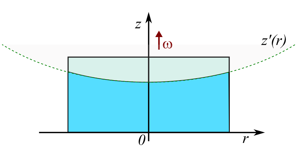
Figure 1: A liquid in a prismatic container with a free surface, $z^{\prime}(r)$, mounted on a rotating table with angular velocity $\omega$ displays a parabolic shape. The figure also indicates the definition of the coordinate axes in the relative system.

Under these assumptions, the velocity field is that of a rigid body and can be expressed as $\vec{u}=\omega r\hat{\theta}$ while the acceleration $\vec{a}=-\omega^{2}r\hat{r}$. To obtain the pressure field, after substituting these expressions in the Eq. (1) we obtain

$$-\omega^{2}r\hat{r}=-\frac{\nabla p}{\rho}-g\hat{z}.$$ (2)

where in the case of an axisymmetric field the gradient can be written as

$$\nabla p=\frac{\partial p}{\partial r}\hat{r}+\frac{\partial p}{\partial z}\hat{z}.$$ (3)

The pressure field can be easily integrated to obtain

$$p(r,z)=-\rho gz+\frac{\rho\omega^{2}r^{2}}{2}+C$$ (4)

where $C$ is a constant of integration with dimensions of pressure. The equation of the free surface, $z^{\prime}(r)$, is obtained using the constraint that the pressure corresponds to the atmospheric pressure $p_{atm}$ and results

$$z^{\prime}(r)=\frac{r^{2}\omega^{2}}{2g}-\frac{p_{atm}}{\rho g}+\frac{C}{\rho g}.$$ (5)

The constant $C$ can be obtained using the mass conservation and the fact that the fluid is incompressible,

$$HL=2\int_{0}^{L/2}{z^{\prime}(r)dr}=2\int_{0}^{L/2}{\left(\frac{r^{2}\omega^{2}}{2g}-\frac{p_{atm}}{\rho g}+\frac{C}{\rho g}\right)}dr.$$ (6)

Performing the integral we get the expression for $C$

$$C=p_{atm}+\rho gH-\frac{\rho\omega^{2}L^{2}}{12}.$$ (7)

Finally, the pressure field inside the fluid can be expressed as

$$p(r,z)=p_{atm}+\rho g(H-z)+\frac{\rho\omega^{2}}{2}\left(r^{2}-\frac{L^{2}}{24}\right)$$ (8)

where we can appreciate static and dynamics contributions. The free surface can be finally expressed as

$$z^{\prime}(r)=H-\frac{\omega^{2}}{2g}\left(\frac{L^{2}}{12}-r^{2}\right)$$ (9)

We notice that the concavity and the location of the vertex of the parabole depend on the angular velocity. The vertex of the parabole, given by $r=0$ is located at

$$z_{v}=H-\frac{\omega^{2}L^{2}}{24g}.$$ (10)

When the angular velocity is $\omega\geq\sqrt{24gH}/L$ the parabole vertex reaches the bottom of the container and these expressions are not longer valid. It is also interesting that there are two nodal points given by $z^{\prime}(r_{0})=H$ with $r_{0}=\pm L/\sqrt{12}$ that always belong to the free surface.

III Experimental set-up and data processing

The experimental setup shown in Fig. 2 consists of a prismatic container and a smartphone, model LG-G2 (with digital camera and built-in gyroscope), both of them fixed to a rotating table. The dimensions of the container containing dyed water were $25$ cm width, $15$ cm height and $2$ cm thickness. The rotating table was powered by a DC motor so the rotational speed could be adjusted by varying the voltage applied to the motor.

Initially, with the rotating table at rest we turn on the video camera and we start recording the measures provided with the gyroscope and proximity sensors with the Androsensor app. To synchronize the video and the and data provided by the app, we cover a few seconds simultaneously the lens of the camera and the proximity sensor. In this way we obtain a common time reference for the video and sensor data.

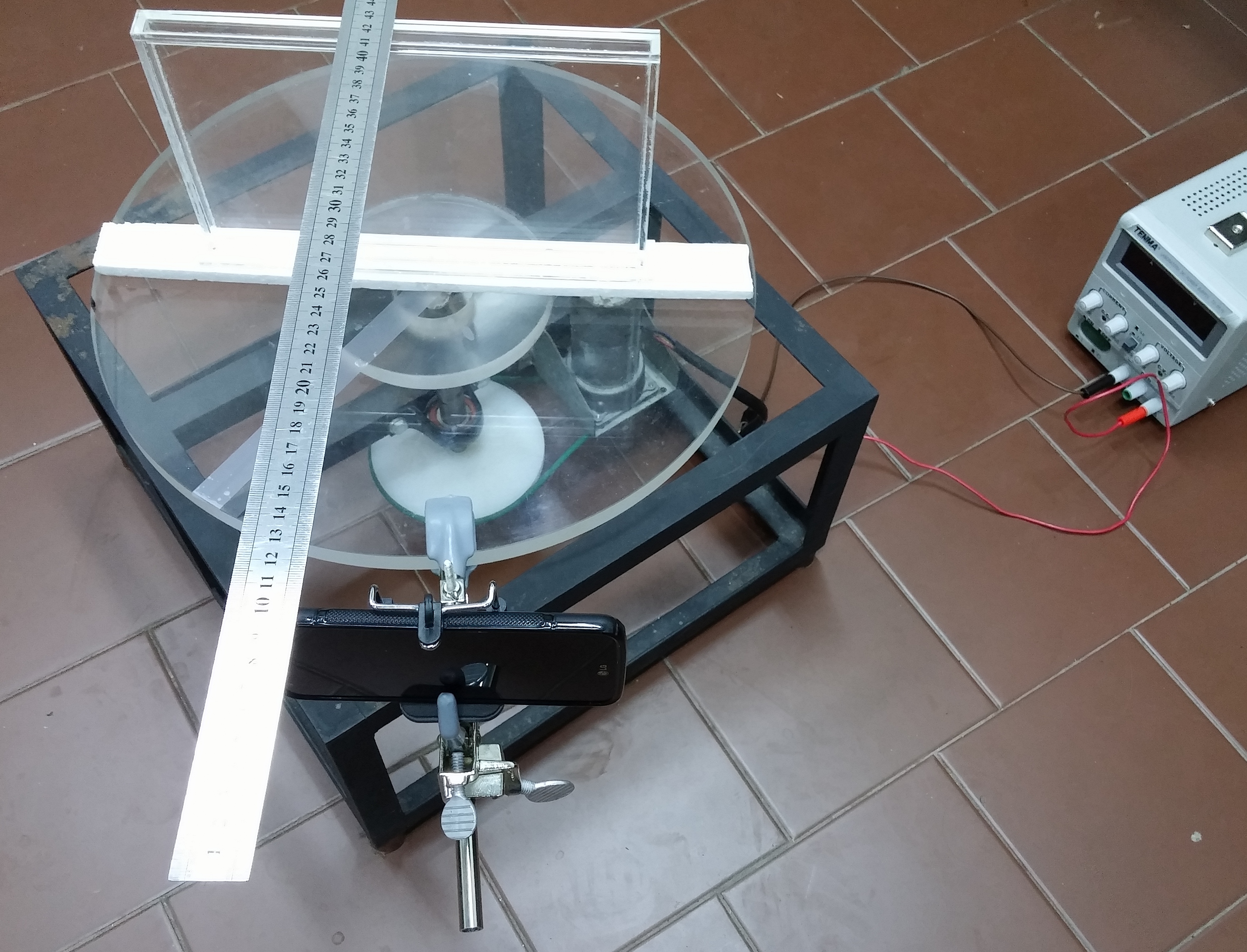
Figure 2: Experimental set-up composed of a narrow container mounted on a rotatory table. The smartphone, also fixed to the rotating system, supplies both the video of the of the time-evolving surface and the angular velocity obtained with the gyroscope.

Then, we turn on the power supply and the rotating table starts rotating. Throughout the experiment the power supply is slowly increased by small jumps and so does the angular velocity. Figure 3 shows the temporal evolution of the angular velocity. The blue arrow indicates the time used to synchronize the video and the sensor data. By the end of the experiment both files, video and sensor data, are transferred to a computer. The accompanying video abstract shows a synopsis of the experimental video. The video is available at https://youtu.be/6SsX16rNoVE.

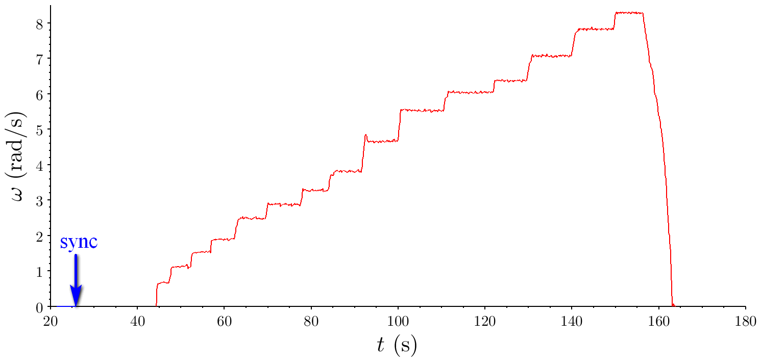
Figure 3: Temporal evolution of the angular velocity. The appreciable jumps are produced by the operator regulating the DC power supply. The blue arrow indicates the instant in which the hand uncover the camera and the proximity sensor to register a mark to synchronize the video and the gyroscope sensor.

To analyze the characteristics of the time-evolving surface, firstly, we extract the individual frames from the digital video. Next, we select 15 frames, corresponding to different values of the angular velocities displayed in Fig. 3. Each frame was analyzed with the video analysis software Tracker brown2009tracker . Several points, tipically 8, on the interface were manually labeled and, then, we perform a parabolic fit, $y=Ax^{2}+Bx+C$. The coefficient $A$ corresponds to the concavity of the parabole. From the coefficients $B$ and $C$ the height of the vertex, $H=-B^{2}/(4A)$, can be readily obtained.

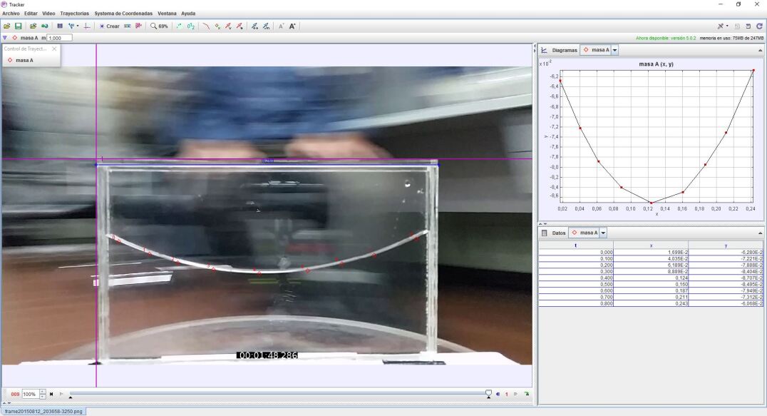
Figure 4: Tracker screen-shot showing one frame of the digital video with the free surface and the points selected (left). The right panel shows the parabolic shape and the coordinates of the selected points.

IV Results

After the data were processed, we compared the results for the concavity and the height of the parabole with the model prediction. Figure 5 shows the experimental relationship between the concavity of the parabole and the angular velocity and the model prediction. The slope of the linear fit $20.16(4)$ m·rad²/s², according to Eq. 9, is with good agreement $2g$.

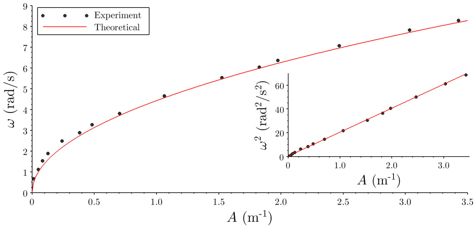
Figure 5: Relationship between the angular velocity and the concavity of the fluid surface fitted to a parabole. The points indicate the experimental results and the solid line the model prediction. The slope of the linear fit shown in inset is $20.16(4)$ m·rad²/s².

The height of the parabole vertex as a function angular velocity squared is plotted in Figure 6. The slope of the linear fit results $-0.27(1)$ mm·s²/rad² which is very similar to the value, according to Eq. 10, given by the model $-L^{2}/24g=-0.2655(5)$ mm·s²/rad². In addition, the intercept corresponds to the water level with the rotating table at rest. In the experiment, the value obtained is $-7.72(3)$cm while the direct value obtained measuring directly on the image is $-7.6(2)$ cm.

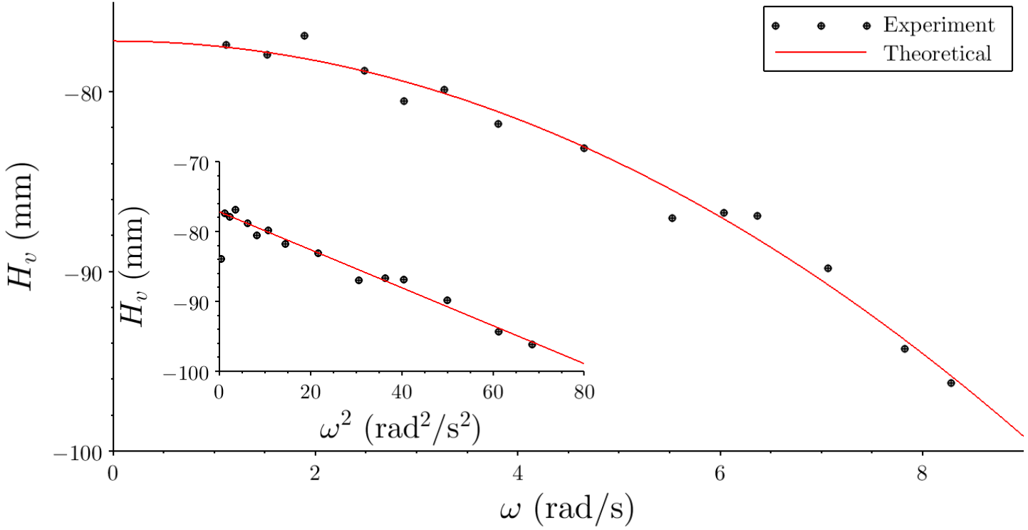
Figure 6: Height of the parabole vertex as a function of the angular velocity squared. The red line indicates a linear fit (slope $-0.27(1)$ mm·s²/rad² and intercept $-7.72(3)$) . The leftmost point which corresponds to a small angular velocity (and therefore present a great uncertainty) was not taken into account in the linear fit shown in the inset.

V Conclusions and Prospects

The present proposal aims at experimenting with the free surface of a liquid rotating with a time dependent angular velocity. Thanks to a smartphone both the shape of the surface and the angular velocity are simultaneously measured. Using video analysis software we obtain the coefficients of the parabolic profile which can be related to the angular velocity, the gravitational acceleration and the water level with the rotating table at rest. The present experiment yields very good agreement with the theoretical model. This simple and inexpensive proposal provides an opportunity for students to engage with challenging aspects of fluid dynamics without sophisticated or expensive equipment.

- (1) Frank M White. Fluid mechanics, 2003.
- (2) Erlend H Graf. Apparatus for the study of uniform circular motion in a liquid. The Physics Teacher, 35(7):427–430, 1997.
- (3) Andréas Sundström and Tom Adawi. Measuring g using a rotating liquid mirror: enhancing laboratory learning. Physics Education, 51(5):053004, 2016.
- (4) Alexsandro Pereira de Pereira and Lara Elena Sobreira Gomes. Rotating the haven of fixed stars: a simulation of mach’s principle. Physics Education, 51(5):055016, 2016.
- (5) Carl-Olof Fägerlind and Ann-Marie Pendrill. Liquid in accelerated motion. Physics Education, 50(6):648, 2015.
- (6) Fernando Tornaría, Martín Monteiro, and Arturo C Marti. Understanding coffee spills using a smartphone. The Physics Teacher, 52(8):502–503, 2014.
- (7) Martín Monteiro, Cecilia Cabeza, Arturo C Marti, Patrik Vogt, and Jochen Kuhn. Angular velocity and centripetal acceleration relationship. The Physics Teacher, 52(5):312–313, 2014.
- (8) Martín Monteiro, Cecilia Cabeza, and Arturo C Martí. Exploring phase space using smartphone acceleration and rotation sensors simultaneously. European Journal of Physics, 35(4):045013, 2014.
- (9) Martín Monteiro, Patrik Vogt, Cecilia Stari, Cecilia Cabeza, and Arturo C. Marti. Exploring the atmosphere using smartphones. The Physics Teacher, 54(5):308–309, 2016.
- (10) Martín Monteiro, Cecilia Stari, Cecilia Cabeza, and Arturo C Martí. The polarization of light and malus’ law using smartphones. The Physics Teacher, 55(5):264–266, 2017.
- (11) Martín Monteiro, Cecilia Stari, Cecilia Cabeza, and Arturo C Marti. Magnetic field ‘flyby’ measurement using a smartphone’s magnetometer and accelerometer simultaneously. The Physics Teacher, 55(9):580–581, 2017.
- (12) D Brown. Tracker: Free video analysis and modeling tool for physics education, June 2014.